Fabrizio D’Errico _______________________________

Lecture Notes in Applied Metallurgy for the course held at Politecnico di Milano for the Master

of Science (MS) Degree in Mechanical Engineering This booklet is based on bibliography of the course. Several parts of this booklet, as well as pic-tures and tables, have been freely taken from the original text books in the selected bibliography of the course. This booklet is provided by the teacher for internal use only to the students at-tending the course of “Applied Metallurgy”, course of the M.Sc. in Mech. Eng. at Politecnico di Milano. No other external uses and/or scopes that are out of preparation to final exam are therefore al-lowed. Any other different uses by the students shall be under their own responsibility.

2

Chapter 1 - Resuming basic principles of metallurgy ........................................ 3

Vacancies, interstitial spaces and grain boundaries as drive-force for diffusion in metals ............................................................................................... 14

Elastic and plastic deformation in metal by micromechanical models ........... 24

Mechanisms of Strengthening in Metals ........................................................... 36 Strengthening by grain size reduction ............................................................. 36 Solid solution strengthening ............................................................................ 39 Strain hardening .............................................................................................. 41 Phase boundaries as strengthening sources .................................................... 44

Grain Growth, Recovery and Recrystallization ............................................... 47 Recovery .......................................................................................................... 47 Grain growth ................................................................................................... 48 Recrystallization .............................................................................................. 50

Mechanical behavior of metals by macroscopic approach .............................. 53 Tensile test ....................................................................................................... 53 Ductility ........................................................................................................... 56 Resilience ......................................................................................................... 56 Toughness ........................................................................................................ 57 Hardness .......................................................................................................... 59

Resuming the main contents, defining the main paradigm for mechanical response of metals ................................................................................................ 60

Microstructural Features of Fracture in Metallic Materials ........................... 64

Chapter 2 - Damage mechanisms and root cause failure analysis basics ....... 71

3

Chapter 1 - Resuming basic principles of metallurgy

Introduction Some of the important properties of solid materials depend on geometrical atomic arrangements, and also the interactions that exist among constituent atoms or mol-ecules. Several fundamental and important concepts— namely, atomic structure, electron configurations in atoms are here reviewed briefly (for more details you may refer to: William D. Callister, Materials Science and engineering: an intro-duction - 7. ed. - New York: John Wiley & sons, 2007; F.C. Campbell, Metallurgy and Engineering Alloys, ASM International, 2008). Atomic Structure and Interatomic Bonding Bohr atomic model, in which electrons are assumed to revolve around the atomic nucleus in discrete orbitals, and the position of any particular electron is more or less well defined in terms of its orbital. This model of the atom is represented in Figure 1.1a.

(a) (b)

Figure 1.1 – (a) A schematic representation of the Bohr atom; (b) covalent bonding requires that elec-trons be shared between atoms in such a way that each atom has its outer sp orbital filled. In silicon, with a valence of four, four covalent bonds must be formed. The electron configuration or structure of an atom represents the manner in which electron states—values of energy that are permitted for electrons states are occu-pied. Valence electrons are those ones that occupy the outermost shell: these elec-trons are extremely important for establishing the bonding between atoms. And bonding between atoms are necessary to form atomic and molecular aggregates. This implies many of the physical and chemical properties of solids are based on these valence electrons.

4

The basics of atomic bonding are best illustrated by considering how two isolated atoms interact as they are brought close together from an infinite separation (Fig. 1.2). At large distances, attraction forces exerted between positive nucleus of one atom and the negative electrons of the other atom are negligible (mutual attrac-tion): this depend on the fact the two atoms are too far apart to have an influence on each other. At small separation distances, each atom can actually exerts forces on the other, but when distance decrease too much, namely nuclei get close, repul-sive forces between positive nuclei surpass attraction force. These counteracting forces, attractive FA and repulsive FR, and the magnitude of each depends on the separation or interatomic distance r (refer to Figure 1.2). The entity of attractive force FA obviously shall depend on the particular type of bonding that exists be-tween the two atoms, as discussed in brief above. In Fig. 1.2b the potential energy is shown (as integral of bonding force ʃ F·dr ).

Figure 1.2 - (a) The dependence of repulsive, attractive, and net forces on interatomic sepa-ration for two isolated atoms. (b) The dependence of repulsive, attractive, and net potential energies on interatomic separation for two isolated atoms.

5

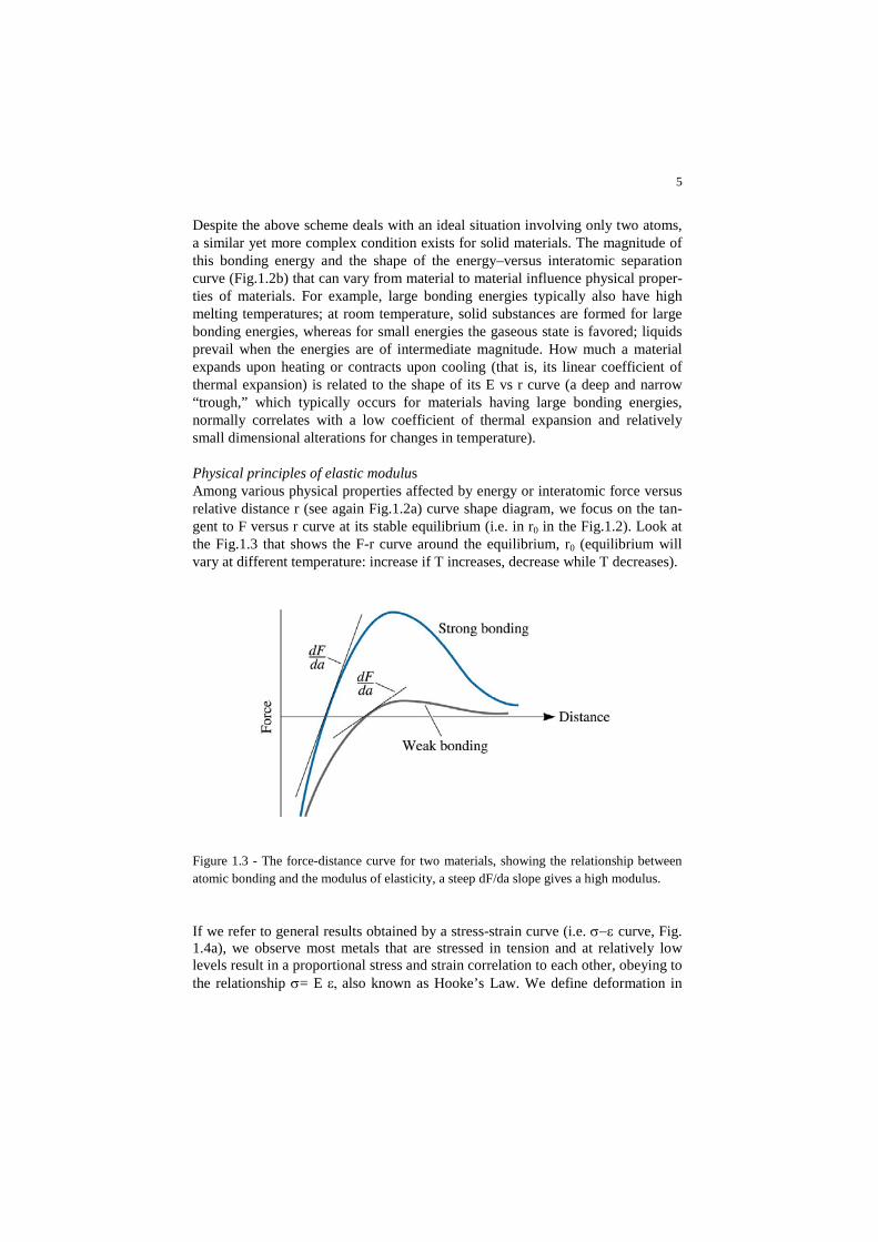
Despite the above scheme deals with an ideal situation involving only two atoms, a similar yet more complex condition exists for solid materials. The magnitude of this bonding energy and the shape of the energy–versus interatomic separation curve (Fig.1.2b) that can vary from material to material influence physical proper-ties of materials. For example, large bonding energies typically also have high melting temperatures; at room temperature, solid substances are formed for large bonding energies, whereas for small energies the gaseous state is favored; liquids prevail when the energies are of intermediate magnitude. How much a material expands upon heating or contracts upon cooling (that is, its linear coefficient of thermal expansion) is related to the shape of its E vs r curve (a deep and narrow “trough,” which typically occurs for materials having large bonding energies, normally correlates with a low coefficient of thermal expansion and relatively small dimensional alterations for changes in temperature). Physical principles of elastic modulus Among various physical properties affected by energy or interatomic force versus relative distance r (see again Fig.1.2a) curve shape diagram, we focus on the tan-gent to F versus r curve at its stable equilibrium (i.e. in r0 in the Fig.1.2). Look at the Fig.1.3 that shows the F-r curve around the equilibrium, r0 (equilibrium will vary at different temperature: increase if T increases, decrease while T decreases).

Figure 1.3 - The force-distance curve for two materials, showing the relationship between atomic bonding and the modulus of elasticity, a steep dF/da slope gives a high modulus. If we refer to general results obtained by a stress-strain curve (i.e. σ−ε curve, Fig. 1.4a), we observe most metals that are stressed in tension and at relatively low levels result in a proportional stress and strain correlation to each other, obeying to the relationship σ= E ε, also known as Hooke’s Law. We define deformation in

6

which stress and strain are proportional as elastic deformation (a nonpermanent deformation) since each loading cycle performed in this stress-strain curve “re-gion” is fully reversible (by unloading, the piece returns to its original shape).

(a) (b)

Figure 1.4 – (a) Typical engineering stress–strain behavior to fracture, point F; (b) a detail of the stress-strain curve in the proportionality regime. On an atomic scale, thus referring again to Fig.1.3, macroscopic elastic strain is manifested as small changes in the interatomic spacing and the stretching of inter-atomic bonds. As a consequence, the magnitude of the modulus of elasticity is a measure of the resistance to separation of adjacent atoms, that is, the interatomic bonding forces. This modulus is proportional to the slope of the interatomic force–separation curve (Figure 1.3) at the equilibrium, and it is a physical properties of material class: it does mostly depend on atomic bonding force of crystal lattice of metals, over a very low influence of varying chemical analysis (steels exhibits atomic bonding force higher than aluminum, so its Young Modulus is higher; Young Modulus of any steels slightly varies in the range 200.000 – 220.000 MPa). Atomic arrangements of metals During melting phase, the energy introduced by heating causes vibration energy1 of atoms to decrease. By opposite reasoning we can say that increasing vibration energy causes progressively equilibrium distance r0 to increase. The material, if it is solid, remains in this state till the equilibrium distance that is increased by in-

1 Atoms vibrates around their equilibrium r0 position at any temperature; at -273 K vibration ceases.

7

creasing temperature (consider that heating up provides energy for increase atom vibration) is lower than low-bonding energy regime (see again Fig.1.2b: as intera-tomic atom distance increases, attractive force, i.e. bonding energy decreases). If atoms reaches high interatomic distance, their mutual attractive force decreases and atoms separate each other. While this phenomenon happens in metal, it is ob-serve a change in status of aggregation: it passes from solid to liquid state. Now, proceed again in back track: cool down temperature of metal that is provid-ed in molten state. The vibration energy of atoms progressively decreases, till some atoms can attract each others. These early movements make some atoms to link each others, and some nuclei of solidified materials appears in the melting phase (see Fig.1.5a)

Figure 1.5 - Schematic diagrams of the various stages in the solidification of a polycrystal-line material; the square grids depict unit cells. (a) Small crystallite nuclei. (b) Growth of the crystallites; the obstruction of some grains that are adjacent to one another is also shown. (c) Upon completion of solidification, grains having irregular shapes have formed. (d) The grain structure as it would appear under the microscope; dark lines are the grain boundaries. What distinguishes metals, some polymers and many ceramics is that when solid state is reached, atoms occupies regular ordering of atoms that extends through the material (Fig.1.5b and c). Particularly here we refer to metals.

8

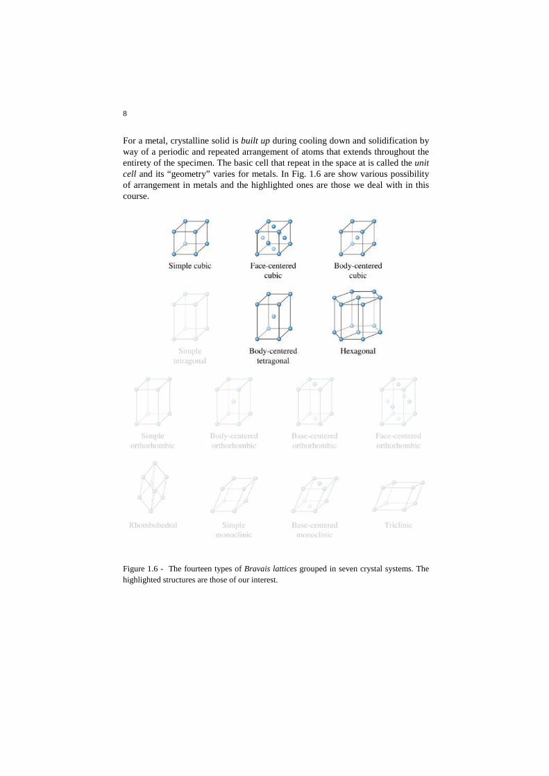
For a metal, crystalline solid is built up during cooling down and solidification by way of a periodic and repeated arrangement of atoms that extends throughout the entirety of the specimen. The basic cell that repeat in the space at is called the unit cell and its “geometry” varies for metals. In Fig. 1.6 are show various possibility of arrangement in metals and the highlighted ones are those we deal with in this course.

Figure 1.6 - The fourteen types of Bravais lattices grouped in seven crystal systems. The highlighted structures are those of our interest.

9

The representation in Fig.1.6 is just schematic; in reality, the lattice structure is made up by atoms that get close each other, compacting and packing in the unit cell above illustrated. In Fig.1.7 is shown the more real structure of a face cen-tered cubic, or FCC, unit cell (Fig.1.7a) compared with the schematic representa-tion (Fig.1.7b) of unit cell, and how the unit cells combine in the space to form solid material (namely, each single grain of Fig.1.5).

Fig.1.7 - For the face centered cubic crystal structure, (a) a “hard sphere” unit cell represen-tation, (b) a reduced-sphere unit cell, and (c) an aggregate of many atoms. Now, imagine to start from the scheme in Fig.1.7b made of ping pong balls at the corner and in center of 6 faces of the cube, and pack as you can, trying to realize by outer uniform compression a compact cube. What happens is that some spaces will remain in your compacted cube. These spaces we call interstitial spaces, or sites. In Fig.1.8, for example, are shown the interstitial spaces present in three type of unit cells. In Fig.1.9 the octahedral site inside the face centered cubic cell.

10

Figure 1.8 - The location of the interstitial sites in cubic unit cells. Only representative sites are shown. The name of the site (e.g. octahedral, tetrahedral, etc.) depends on its location in the

Figure 1.9 - The location of the octahedral site in a face centered cubic unit cell.

Imperfections in the Atomic and Ionic Arrangements Thus far it has been tacitly assumed that perfect order exists throughout crystalline materials on an atomic scale. However, such an idealized solid does not exist. Meanwhile cooled down, a metal solidifies by solid nuclei formation (see again Fig.5) and grain growth. It is worth of noticing that the simplified scheme of solid-ification in Fig.5 actually it is to be considered as a low magnification representa-tion; if you imagine to observe by an “atomic microscope” (we imagine we holds such a marvelous equipment) nuclei that are forming inside liquid phase as illus-trated in Fig.5, actually we have to consider they are building up meanwhile atoms by atoms occupy fixed position inside the specific unit cell. Each metal, we know, has its own specific atomic arrangement – it is just like the DNA code for organ-isms - that mainly depends on the base element, e.g. body cubic centered, BCC,

11

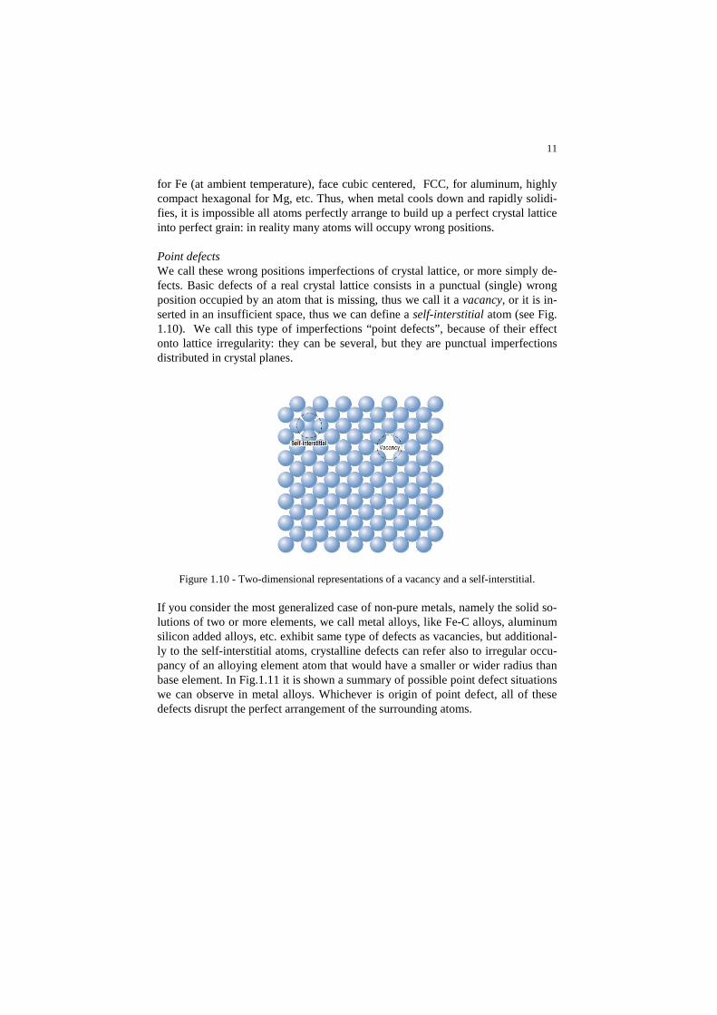
for Fe (at ambient temperature), face cubic centered, FCC, for aluminum, highly compact hexagonal for Mg, etc. Thus, when metal cools down and rapidly solidi-fies, it is impossible all atoms perfectly arrange to build up a perfect crystal lattice into perfect grain: in reality many atoms will occupy wrong positions. Point defects We call these wrong positions imperfections of crystal lattice, or more simply de-fects. Basic defects of a real crystal lattice consists in a punctual (single) wrong position occupied by an atom that is missing, thus we call it a vacancy, or it is in-serted in an insufficient space, thus we can define a self-interstitial atom (see Fig. 1.10). We call this type of imperfections “point defects”, because of their effect onto lattice irregularity: they can be several, but they are punctual imperfections distributed in crystal planes.

Figure 1.10 - Two-dimensional representations of a vacancy and a self-interstitial. If you consider the most generalized case of non-pure metals, namely the solid so-lutions of two or more elements, we call metal alloys, like Fe-C alloys, aluminum silicon added alloys, etc. exhibit same type of defects as vacancies, but additional-ly to the self-interstitial atoms, crystalline defects can refer also to irregular occu-pancy of an alloying element atom that would have a smaller or wider radius than base element. In Fig.1.11 it is shown a summary of possible point defect situations we can observe in metal alloys. Whichever is origin of point defect, all of these defects disrupt the perfect arrangement of the surrounding atoms.

12

Figure 1.11 - Point defects: (a) vacancy, (b) interstitial atom, (c) small substitutional atom, (d) large substitutional atom, Interfacial defects: grain boundary Grain boundary is represented schematically from an atomic perspective in Figure 1.14. Within the boundary region, which is probably just several atom distances wide, there is some atomic mismatch in a transition from the crystalline orienta-tion of one grain to that of an adjacent one. Various degrees of crystallographic misalignment between adjacent grains are possible (Figure 1.15).When this orien-tation mismatch is slight, on the order of a few degrees, then the term small- (or low-) angle grain boundary is used. These boundaries can be described in terms of dislocation arrays. One simple small-angle grain boundary is formed when edge dislocations are aligned in the manner of Figure 4.8. This type is called a tilt boundary; the angle of misorientation, θ, is also indicated in the figure. When the angle of misorientation is parallel to the boundary, a twist boundary results, which can be described by an array of screw dislocations.

13

Figure 1.14 – Schematic diagram showing small and high-angle grain boundaries and the adjacent atom positions.

Figure 1.15 – A tilt boundary having an angle of misorientation θ, results from an align-ment of edge dislocations. As special type of grain boundary twin boundary is worth of noticing: it exhibits a specific mirror lattice symmetry (it depends on crystal lattice). Thus atoms on one

14

side of the boundary are located in mirror-image positions of the atoms on the oth-er side (Figure 1.16).

Figure 1.16 Schematic diagram showing a twin plane or boundary and the adja-cent atom positions (colored circles).

Vacancies, interstitial spaces and grain boundaries as drive-force for diffusion in metals

Firstly we address the diffusion by the phenomenological point of view. Let us see the scheme in Fig. 1.16. The phenomenon of diffusion may be demonstrated with the use of a diffusion couple, which is formed by joining bars of two different metals together so that there is intimate contact between the two faces; this is illus-trated for copper and nickel. which includes schematic representations of atom po-sitions and composition across the interface. This couple is heated for an extended period at an elevated temperature (but below the melting temperature of both met-als) and cooled to room temperature. Chemical analysis will reveal a condition similar to that represented in Figure 1.15 —namely, pure copper and nickel at the two extremities of the couple, separated by an alloyed region. Concentration of both metals vary with position as shown in Figure 1.15f. This result indicates that copper atoms have migrated or diffused into the nickel, and that nickel has dif-fused into copper. This process, whereby atoms of one metal diffuse into another, is termed inter-diffusion, or impurity diffusion. There is a net drift or transport of atoms from high- to low-concentration regions. Diffusion also occurs for pure metals, but all atoms exchanging positions are of the same type; this is termed self-diffusion. Of course, self-diffusion is not nor-mally subject to observation by noting compositional changes. This was the experiment, to allow us to observe results of diffusion: but which are mechanisms that causes diffusion into metals?

15

Figure 1.16 – Start experiment time: (a) a copper–nickel diffusion couple before a high-temperature heat treatment; (b) schematic representations of Cu (red circles) and Ni (blue circles) atom locations within the diffusion couple; (c) concentrations of copper and nickel as a function of position across the couple; (d) the copper–nickel diffusion couple after a high-temperature heat treatment, showing the alloyed diffusion zone; (e) schematic repre-sentations of Cu (red circles) and Ni (blue circles) atom locations within the couple; (f) Concentrations of copper and nickel as a function of position across the couple. Mechanisms of diffusion into metal From an atomic perspective, diffusion is just the stepwise migration of atoms from lattice site to lattice site. In fact, the atoms in solid materials are in constant mo-tion, rapidly changing positions. For an atom to make such a move, two conditions must be met: (1) there must be an empty adjacent site, and (2) the atom must have sufficient energy to break bonds with its neighbor atoms and then cause some lat-tice distortion during the displacement. As stated, this energy is vibrational in na-ture until cooling down metals to -273 K. At a specific temperature some small fraction of the total number of atoms is capable of diffusive motion, by virtue of the magnitudes of their vibrational energies. This fraction increases with rising temperature. Several different models for this atomic motion have been proposed; of these pos-sibilities, two dominate for metallic diffusion.

(a)

(b)

(c)

(d)

(e)

(f)

16

– Vacancy Diffusion: involves the interchange of an atom from a normal lat-tice position to an adjacent vacant lattice site or vacancy, as represented schematically in Fig.1.17a. This process of course necessitates the pres-ence of vacancies, and the extent to which vacancy diffusion can occur is a function of the number of these defects that are present.

– Interstitial Diffusion: The second type of diffusion involves atoms that mi-grate from an interstitial position to a neighboring one that is empty; this mechanism is found for interdiffusion of impurities and very small-radius atoms (such as hydrogen, carbon, nitrogen, and oxygen) that are small enough to fit into the interstitial positions and move (Fig.1.17b). In most metal alloys, interstitial diffusion occurs much more rapidly than diffusion by the vacancy mode, because the interstitial atoms are smaller and thus more mobile. Furthermore, there are more empty interstitial positions than vacancies; hence, the probability of interstitial atomic movement is greater than for vacancy diffusion.

Figure 1.17 – Schematic representations of (a) vacancy diffusion and (b) interstitial diffusion.

17

Box - Modeling of diffusion into metals Diffusion is a time-dependent process—that is, in a macroscopic sense, the quanti-ty of an element that is transported within another is a function of time. Often it is necessary to know how fast diffusion occurs, or the rate of mass transfer. This rate is frequently expressed as a diffusion flux (J), defined as the mass (or, equivalently, the number of atoms) M diffusing through and perpendicular to a unit cross-sectional area of solid per unit of time. In mathematical form, this may be repre-sented as:

(𝑒𝑒𝑒𝑒. 1.1) 𝐽𝐽 = 𝑀𝑀𝐴𝐴 ∙ 𝑡𝑡

where A denotes the area across which diffusion is occurring and t is the elapsed diffusion time. In differential form, this expression becomes:

(𝑒𝑒𝑒𝑒. 1.2) 𝐽𝐽 = 1𝐴𝐴𝑑𝑑𝑀𝑀𝑑𝑑𝑡𝑡

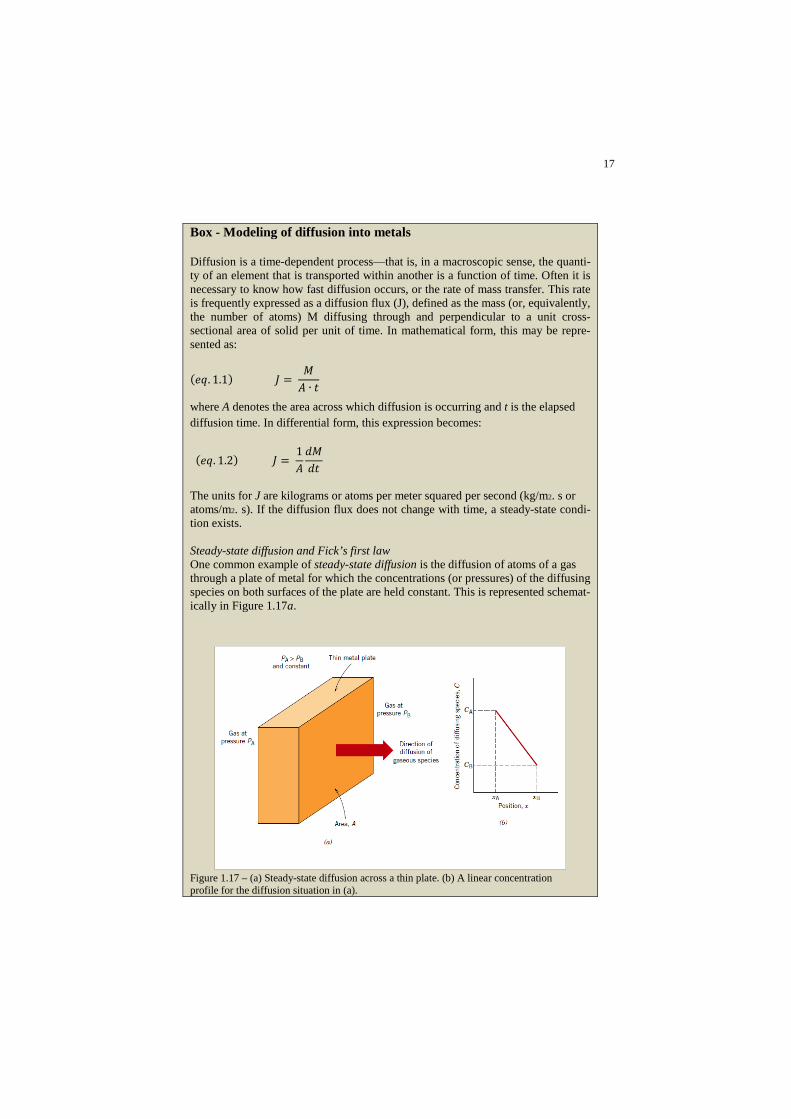
The units for J are kilograms or atoms per meter squared per second (kg/m2. s or atoms/m2. s). If the diffusion flux does not change with time, a steady-state condi-tion exists. Steady-state diffusion and Fick’s first law One common example of steady-state diffusion is the diffusion of atoms of a gas through a plate of metal for which the concentrations (or pressures) of the diffusing species on both surfaces of the plate are held constant. This is represented schemat-ically in Figure 1.17a.

Figure 1.17 – (a) Steady-state diffusion across a thin plate. (b) A linear concentration profile for the diffusion situation in (a).

18

When concentration C is plotted versus position (or distance) within the solid x, the resulting curve is termed the concentration profile; the slope at a particular point on this curve is the concentration gradient:

(𝑒𝑒𝑒𝑒. 1.3) 𝑐𝑐𝑐𝑐𝑐𝑐𝑐𝑐𝑒𝑒𝑐𝑐𝑡𝑡𝑐𝑐𝑐𝑐𝑡𝑡𝑐𝑐𝑐𝑐𝑐𝑐 𝑔𝑔𝑐𝑐𝑐𝑐𝑑𝑑𝑐𝑐𝑒𝑒𝑐𝑐𝑡𝑡 =𝑑𝑑𝑑𝑑𝑑𝑑𝑑𝑑

In the present experiment, the concentration profile is assumed to be linear, as de-picted in Figure 1.17b, and:

(𝑒𝑒𝑒𝑒. 1.4) 𝑐𝑐𝑐𝑐𝑐𝑐𝑐𝑐𝑒𝑒𝑐𝑐𝑡𝑡𝑐𝑐𝑐𝑐𝑡𝑡𝑐𝑐𝑐𝑐𝑐𝑐 𝑔𝑔𝑐𝑐𝑐𝑐𝑑𝑑𝑐𝑐𝑒𝑒𝑐𝑐𝑡𝑡 =∆𝑑𝑑∆𝑑𝑑 =

𝑑𝑑𝐴𝐴 − 𝑑𝑑𝐵𝐵𝑑𝑑𝐴𝐴 − 𝑑𝑑𝐵𝐵

The mathematics of steady-state diffusion in a single (x) direction is relatively simple, in that the flux is proportional to the concentration gradient through the expression:

(𝑒𝑒𝑒𝑒. 1.5) 𝐽𝐽 = −𝐷𝐷 𝑑𝑑𝑑𝑑𝑑𝑑𝑑𝑑

The constant of proportionality D is called the diffusion coefficient, which is ex-pressed in square meters per second. The negative sign in this expression indicates that the direction of diffusion is down the concentration gradient, from a high to a low concentration. Equation 1.5 is sometimes called Fick’s first law. When diffu-sion is according to Equation 5.3, the concentration gradient is the driving force.

Non-steady state diffusion and Fick’s second law The diffusion flux and the concentration gradient at some particular point in a solid vary with time, with a net accumulation or depletion of the diffusing species result-ing. This is illustrated in Figure 1.18, which shows concentration profiles at three different diffusion times. In this case, instead the Fick’s first law, a partial differen-tial equation is used to more precisely model the phenomenon: (𝑒𝑒𝑒𝑒. 1.6) 𝜕𝜕𝜕𝜕

𝜕𝜕𝜕𝜕= 𝜕𝜕

𝑥𝑥(𝐷𝐷 𝜕𝜕𝜕𝜕

𝜕𝜕𝑥𝑥)

The above equation is known as Fick’s second law. If the diffusion coefficient is independent of composition (which should be verified for each particular diffusion situation), Equation 1.6 simplifies to:

(𝑒𝑒𝑒𝑒. 1.7) 𝜕𝜕𝑑𝑑𝜕𝜕𝑡𝑡 = 𝐷𝐷

𝜕𝜕2𝑑𝑑𝜕𝜕𝑑𝑑

19

Solutions to this expression (concentration in terms of both position and time) are possible when physically meaningful boundary conditions are specified.

Figure 1.18 - Concentration profiles for nonsteady-state diffusion taken at three different times, t1, t2, and t3.

The use of Erf Function in modeling diffusion Frequently, the source of the diffusing species is a gas phase, the partial pressure of which is maintained at a constant value. Furthermore, the following assumptions are made: 1. Before diffusion, any of the diffusing solute atoms in the solid are uniformly 2. distributed with concentration of C0. 3. The value of x at the surface is zero and increases with distance into the solid. 4. The time is taken to be zero the instant before the diffusion process begins.

These boundary conditions are simply stated as For t =0, C= C0 at 0 ≤ x ≤ ∞ For t > 0, C = Cs (the constant surface concentration) at x = 0 C= C0 at x = ∞ Application of these boundary conditions to Equation 1.7 yields the solution:

(𝑒𝑒𝑒𝑒. 1.8) 𝑑𝑑𝑠𝑠 − 𝑑𝑑𝑥𝑥𝑑𝑑𝑠𝑠 − 𝑑𝑑0

= 𝑒𝑒𝑐𝑐𝑒𝑒 �𝑑𝑑

2√𝐷𝐷𝑡𝑡�

Where: o Cs is the surface concentration of gas diffusing into the surface, o Co is the initial concentration of the element in the solid, x is the distance

from the surface, o D is the diffusivity of the solute element in the solvent matrix, and t is time; o erf (error function) is a mathematical function that can be found in standard

mathematical tables, also included in excel function;

20

Case study - Carburization process modeling Assume gas carburizing process conducted on 1020 steel, at 930 °C; Assume that the steel has a nominal carbon content of 0.20%, and the carbon

content at the surface is 0.90%. The diffusion coefficient under these conditions is D930°C =1.28 ·10-11 m2/s The time necessary to increase the carbon content to 0.40% at 0.50mm below

the surface can be calculated in the following manner:

Figure 1.19 – Carbon concentration during carburizing.

21

Internal factors that affect diffusion In the following are listed two main inner factors among various which affect dif-fusion kinetics. Diffusing species: The magnitude of the diffusion coefficient D is indicative of the rate at which atoms diffuse. The diffusing species as well as the host material in-fluence the diffusion coefficient. For example, there is a significant difference in magnitude between self-diffusion and carbon interdiffusion in iron at 500°C, the D value being greater for the carbon interdiffusion (3.0 x 10-21

vs. 2.4 x 10-12 m2/s). This comparison also provides a contrast between rates of diffusion via vacancy and interstitial modes as discussed earlier. Self-diffusion occurs by a vacancy mechanism, whereas carbon diffusion in iron is interstitial. Temperature: Temperature has a most profound influence on the coefficients and diffusion rates. For example, for the self-diffusion of Fe in α-Fe, the diffusion co-efficient increases approximately six orders of magnitude in rising temperature from 500°C to 900°C. The temperature dependence of the diffusion coefficients is:

(eq.1.9) 𝐷𝐷 = 𝐷𝐷0 exp �− 𝑄𝑄𝑑𝑑𝑅𝑅𝑅𝑅�

Where: D0 is a temperature-independent pre-exponential (m2/s) Qd is the activation energy for diffusion (J/mol) R is the gas constant, 8.31 J/mol·K T is the absolute temperature (K) The activation energy may be thought of as that energy required to produce the diffusive motion of one mole of atoms. A large activation energy results in a rela-tively small diffusion coefficient.

Box - Determining D0 and Qd

Taking natural logarithms of Equation 1.9 yields:

(𝑒𝑒𝑒𝑒. 1.10) 𝐿𝐿𝑐𝑐𝑔𝑔 𝐷𝐷 = 𝐿𝐿𝑐𝑐𝑔𝑔 𝐷𝐷0 − Q𝑑𝑑

2.3 𝑅𝑅 �1𝑇𝑇�

Because D0, Qd, and R are all constants, Equation 1.10 takes on the form of an equation of a straight line: y = b+ mx. where y and x are analogous, respectively, to the variables log D and 1/T. Thus, if log D is plotted versus the reciprocal of the absolute temperature, a straight line should result, having slope and intercept

22

of -Qd/2.3R and log D0, respectively. This is the manner in which the values of Qd and D0 are determined experimentally. From such a plot for several alloy systems (Figure 1.20), it may be noted that linear relationships exist for all cases shown.

Figure 1.20 - Plot of the logarithm of the diffusion coefficient versus the reciprocal of ab-solute temperature for several metals.

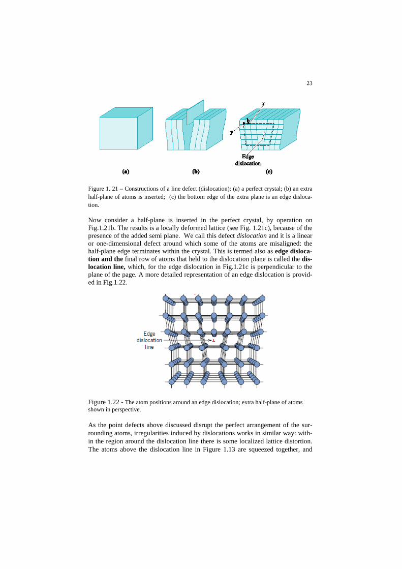
Line defects: dislocations in metals Punctual defects are not the only type of wrong arrangement of atoms inside crys-tal lattice. Several atoms can occupy wrong positions, at the same time. We there-fore talk about the line or plane defect. Let us see what it does mean. Assume to consider a perfect ordered crystal lattice, as it is schematically represented by per-fect cubes link together in a perfect spatial order, as the scheme in Fig.1.21a de-picts.

23

Figure 1. 21 – Constructions of a line defect (dislocation): (a) a perfect crystal; (b) an extra half-plane of atoms is inserted; (c) the bottom edge of the extra plane is an edge disloca-tion. Now consider a half-plane is inserted in the perfect crystal, by operation on Fig.1.21b. The results is a locally deformed lattice (see Fig. 1.21c), because of the presence of the added semi plane. We call this defect dislocation and it is a linear or one-dimensional defect around which some of the atoms are misaligned: the half-plane edge terminates within the crystal. This is termed also as edge disloca-tion and the final row of atoms that held to the dislocation plane is called the dis-location line, which, for the edge dislocation in Fig.1.21c is perpendicular to the plane of the page. A more detailed representation of an edge dislocation is provid-ed in Fig.1.22.

Figure 1.22 - The atom positions around an edge dislocation; extra half-plane of atoms shown in perspective. As the point defects above discussed disrupt the perfect arrangement of the sur-rounding atoms, irregularities induced by dislocations works in similar way: with-in the region around the dislocation line there is some localized lattice distortion. The atoms above the dislocation line in Figure 1.13 are squeezed together, and

24

those below are pulled apart; this is reflected in the slight curvature for the vertical planes of atoms as they bend around this extra half-plane. Elastic and plastic deformation in metal by micromechanical models

Let us consider the scheme in Figure 1.23, representing by micromechanics’ ap-proach a perfect crystal lattice of metal: spheres represent atoms of same specie (thus we deal in this moment with pure metal), no defects, neither vacancies, or dislocations are present. The link (electric bonding we discussed in previous para-graph) between atoms is represented by a spring that exhibits, if loaded in tension, an attractive force (this is in analogy with electric attraction between nuclei and opposite atom’s electrons). Finally, we assume, for the sake of simplicity, that the box-shaped atoms grid that represents the 2D-dimension crystal lattice of our met-al is actually a single grain. This means that square perimeter of the grid in Fig.1.23a actually corresponds to the grain boundary. Now let us apply on this grid a tensile load, as it is illustrated by the arrows in Fig.1.23b. What does it hap-pen to our grid in term of deformation?

Figure 1.23 –(a) Tensile external load applied to perfect crystal lattice; (b) tensile stress leads to elastic deformation, and eventually to (c) a brittle rupture consisting in simultane-ous breaking of atom bonds. Let us proceed reasoning about the assumptions we stated. Each “spring” in the micromechanical model that represents the atom bond obeys to a well-known mechanical relation F=K·x; this means, each spring has same be-havior and same maximum strength. Applying tensile stress, the grid will extend as shown in Fig.1.23b. But, when the load is so high and springs extend too much

(a) (b) (c)

25

that they exceed their own maximum resistance, springs finally break2. Moreover, if one single spring breaks, all the springs distributed in the row perpendicular to the force direction break at the same time (remember that they have same maxi-mum strength, as they are similar). The result in this case is that all the atoms of the grid, from the left side to the right side, detach as Fig.1.23c shows. In other words, the grain (remember the square grid for us represent a single grain) rapidly fracture into two pieces. This is the failure scheme which is usual in brittle materi-als, like ceramics. Think to throw a ceramic piece onto floor: it breaks into two or more separate pieces, with no deformation. We know by experience that metals, usually, when they break exhibit also large deformed surface. The scheme in Fig.1.23 cannot therefore explain the plastic deformation in metals; on the other hand, it can well explain the elastic deformation, as in the next we can understand. Look again at Fig.1.4. We stated initial stage of the stress-strain curve in metal concerns on reversible, or elastic, deformation. Once the load is removed, the specimen recovers original dimension. This is well explained by the microme-chanical model shown in Fig.1.23a, since until tensile load we apply is sufficiently low (i.e. onto macro-mechanical model, this means keeping stress below the Yield Strength, YS), the springs in the “atomic grid” elastically extends. As soon as we remove the load, the grid recovers its original shape. Thus, which way should we modify the micromechanical model to well explain what we macroscopically observe when specimen surpasses the YS and enters in plastic deformation regime? We know in metals, as stress arises above the YS, the elastic regime stage is abandoned, thus metal starts to permanently deform. We now want to seek a micromechanical model that allows us to explain such a plastic regime. Let us consider the same “atomic grid” of Fig.1.13 but now we want to check what happens if we apply a shear stress scheme, instead of the tensile stress, accordingly with the scheme in Fig.1.24.

Figure 1.24 – (a) Shear stress applied to perfect crystal lattice; (b) on certain plane shear stresses can develop and induce atoms in two facing rows to slip. The final shape of the pe-rimeter of the grid irreversibly changes, thus depicting plastic deformation has occurred.

2 You can read this statement as follows: when atoms are separated by a distance that determine attractive force drastically reduces, see Fig. 1.2.

τinternal

(a) (b)

Slip plane

26

By such a stress field, shear stresses develop onto the intermediate plane, as shown in the scheme of Fig.1.14b. Let us for the next that shear stress is higher enough (we’ll better comment how much high it should be), it is capable to make one crystal lattice plane to slip over the opposite one; the result of this movement is clearly shown in Fig.1.24b. The atoms of the upper part of the grid have moved of one step ahead, of the order of an interatomic space. If you imagine to remove the external load, the perimeter of the grid cannot be restored at its original shape. The irreversible deformation has occurred, without implying brittle rupture of atomic bonds. Thus, the plastic deformation in metal can be effectively explained by this micromechanical scheme. But, there is still a but. If we refer to perfect crystal lattice shown in Fig.1.24, dur-ing the slip movement of one step order, 6 atomic bonds have been broken and 5 have been restored. It appears the net balance of energy concerns on 1 atomic bonds, but we need to consider the start of the movement has required in any case external load is sufficient to develop shear stresses capable to break out 6 atom bonds. You should take into account that we’re enormously reducing the scale of a grain to a 36 atoms! But if we consider a grain in reality, the number of atoms from one border to the opposite border is of the order of millions! This means that to realize a very insignificant variation of perimeter of grain, shear stress along the grain should be capable to break millions of atomic bonds, simultaneously, thus recovering this huge quantity of energy as the atoms onto slip plane advance one step (see again the scheme in Fg.1. 24b). This cannot be explainable in reality, since too much high would be the minimum shear stress to activate the slip that no machines on Earth would be adequate to plastically deform metals. From our knowledge of the metallic bond, it is possible to derive a theoretical value for the stress required to produce slip by the simultaneous movement of atoms along a plane in a metallic crystal. However, the strength actually obtained experimentally on single crystals is only about one-thousandth (1/1000) of the theoretical value, assuming simultaneous slip by all atoms on the plane. Obviously, slip does not oc-cur by the simple simultaneous block movement of one layer of atoms sliding over another. The modern concept is that slip occurs by the step-by-step movement of dislocations through the crystal. But, how does it contribute in plastic deformation of metals? Dislocation and plastic deformation in metal Fortunately in metals there are millions of dislocations distributed into crystal lat-tice, as that one shown in the scheme of Fig.1.22. To comprehend how dislocation positively works for plastic deformation, let us consider the scheme in Fig.1.25. When force is applied such that it shears the upper portion of the crystal to the right the plane of atoms above the dislocation can easily establish bonds with the lower plane of atoms to its right, with the result that the dislocation moves one lat-tice spacing at a time. Note that only single bonds are being broken at any one time, rather than the whole row. The atomic distribution is again similar to the ini-tial configuration, and so, the slipping of atom planes can be repeated. The move-

27

ment is much like that of advancing a carpet along a floor by using a wrinkle that is easily propagated down its length. This stress required to cause plastic deformation is orders of magnitude less when dislocations are present than in dislocation-free, perfect crystalline structures.

Figure 1.25 - Line dislocation movement.

If a large number of dislocations move in succession along the same slip plane, the accumulated deformation becomes visible, resulting in macroscopic plastic de-formation. This effect is represented by a simplified scheme in Fig.1.26 represent-ing the macroscopic effect of grain boundary modification into polycrystalline metal. If a large number of dislocations move in succession along the same slip plane, the accumulated deformation becomes visible, resulting in macroscopic plastic deformation.

Figure 1.26 – Permanent deformation occurring at grain boundaries in polycrystalline met-als that reveal macroscopic deformation onto surface of specimen under tensile loading.

No force applied, dislocationinside grain do not move

Force applied, maximum shear stress induces dislocations on 45°

slip planes to move to grainboundary

45°

σ

σ

28

Fig.1.26 also introduces further important key-point: dislocations do not move with the same degree of ease on all crystallographic planes nor in all crystallo-graphic directions. Ordinarily, there are preferred planes, and in these planes, there are specific directions along which dislocation motion can occur. These planes are called slip planes, and the direction of movement is known as the slip direction. The combination of a slip plane and a slip direction forms a slip system Slip planes in metals For a particular crystal structure, the slip plane is that plane having the most dense atomic packing; that is, it has the greatest planar density. The slip direction corre-sponds to the direction, in this plane, that is most closely packed with atoms, that is, has the highest linear density. Consider, for example, the FCC crystal structure, a unit cell of which is shown in Figure 1.27a. There is a set of planes, the {111} family, all of which are closely packed. A (111)-type plane is indicated in the unit cell; in Figure 1.27b, this plane is positioned within the plane of the page, in which atoms are now represented as touching nearest neighbors.

Figure 1.27 – (a) A {111} slip system shown within an FCC unit cell. (b) The (111) plane from (a) and three slip directions (as indicated by arrows) within that plane constitute pos-sible slip systems.

Slip occurs along -type directions within the {111} planes, as indicated by arrows in Figure 1.27. Hence, represents the slip plane and direction combination, or the slip system for FCC. Figure 1.27b demonstrates that a given slip plane may con-tain more than a single slip direction. Thus, several slip systems may exist for a particular crystal structure; the number of independent slip systems represents the different possible combinations of slip planes and directions. For example, for face-centered cubic, there are 12 slip systems: four unique {111} planes and, with-in each plane, three independent directions. The possible slip systems for BCC and HCP crystal structures are listed in Table 1.1. For each of these structures, slip is possible on more than one family of planes

29

(e.g., {110}, {211}, and {321} for BCC). For metals having these two crystal structures, some slip systems are often operable only at elevated temperatures.

Table 1.1. - Slip Systems for Face-Centered Cubic, Body-Centered Cubic, and Hexagonal Close-Packed Metals. Face-centered cubic (fcc) metals have a large number of slip systems (12) and are therefore capable of moderate-to-extensive plastic deformation. Although body-centered cubic (bcc) systems often have up to 12 slip systems, some of them, like steel, exhibit a ductile-to-brittle transition as the temperature is lowered due to the strong temperature sensitivity of their yield strength, which causes them to frac-ture prior to reaching their full potential of plastic deformation. In general, the number of slip systems available for hexagonal close-packed (hcp) metals is less than that for either the fcc or bcc metals, and their plastic deformation is much more restricted. The hcp structure normally has only three to six slip systems, only one-fourth to one-half the available slip systems in fcc. Since plastic deformation takes place by slip, or sliding, on the close-packed planes, the greater the number of slip systems available, the greater the capacity for plastic deformation. Slip in single crystal: the Schmid’s law A further explanation of slip is simplified by treating the process in single crystals, then making the appropriate extension to polycrystalline materials. By mechanics in solid we know that, though an applied stress may be pure tensile (or compres-sive), shear components exist. Existence of shear stress is necessary to activate slip planes, so to move dislocation onto this plane along its slip direction. Howev-er the shear stress acting along this direction shall be sufficiently higher to pro-mote dislocation movement. We need therefore to calculate the projected shear stress along the slip direction of the external tensile force F applied (see again Fig.1.28a), thus compare the value of this shear stress to the minimum shear stress necessary for dislocation movement, or critical shear stress, τc. The former shear stress is called the resolved shear stress, τr and its magnitude depends not only on the applied stress, but also on the orientation of both the slip plane and direc-tion within that plane. To best understand last statement, look at the scheme in

30

Fig.1.28a. Assume the normal, n, of the slip plane lies at an angle, φ, to the tensile axis. The area A of the slip plane considered for all the specimen will be A0/cos φ. Similarly, if the slip plane lies at an angle, λ, to the tensile axis, the component of the axial force, F, acting on the slip direction will be F·cos λ. The resolved shear stress, τr, is then given by: (𝑒𝑒𝑒𝑒. 1.20) 𝜏𝜏𝑟𝑟 = 𝑃𝑃 cos 𝜆𝜆

�𝐴𝐴 cos𝜙𝜙� �= 𝜎𝜎 cos𝜙𝜙 cos 𝜆𝜆

Where σ is the applied stress. If we consider the theoretical case of a single crystal (grain) specimen where the slip direction is orthogonal to tensile stress we applied on specimen (see Fig.1.29), the shear stress τr for the Schmid law is 0: this means that also for high applied tensile stress, resolved shear stress does not develop and any dislocations cannot move. Ultimately, slip of planes cannot occur and plastic deformation cannot occur.

(a) (b)

Figure 1.28 – (a) Tensile test of single crystal and the Schmid’s Law components. (b) If dis-location is present perpendicular onto slip plane, it can be activated, and planes slip.

Figure 1.29 - If a slip plane is perpendicular to applied stress σ , the shear stress τr = 0. Also for high applied stress, no resolved shear stress develop and no dislocation can move. Slip cannot occur, deformation cannot occur.

31

In general, φ + λ ≠ 0 because it need not be the case that the tensile axis, the slip plane normal, and the slip direction all lie in the same plane. A metal single crystal has a number of different slip systems that are capable of operating. The resolved shear stress normally differs for each one because the orientation of each relative to the stress axis (φ and λ angles) also differs. However, one slip system is gener-ally oriented most favorably—that is, has the largest resolved shear stress, τr (max):

(𝑒𝑒𝑒𝑒. 1.21) 𝜏𝜏𝑟𝑟𝑟𝑟𝑟𝑟𝑥𝑥 = 𝜎𝜎𝑦𝑦(cos𝜙𝜙 cos 𝜆𝜆 )𝑟𝑟𝑟𝑟𝑥𝑥 In response to an applied tensile or compressive stress, slip in a single crystal commences on the most favorably oriented slip system when the resolved shear stress reaches a critical value, termed the critical resolved shear stress τcrss; it represents the minimum shear stress required to initiate slip and is a property of the material that determines when yielding occurs. The single crystal plastically deforms or yields when τr (max) = τcrss, and the magnitude of the applied stress required to initiate yielding (i.e., the yield strength σy) is:

(𝑒𝑒𝑒𝑒. 1.22) 𝜎𝜎𝑦𝑦 = 𝜏𝜏𝜕𝜕𝑟𝑟𝑠𝑠𝑠𝑠

(cos𝜙𝜙 cos 𝜆𝜆)𝑚𝑚𝑐𝑐𝑑𝑑

The minimum stress necessary to introduce yielding occurs when a single crystal is oriented such that φ = λ = 45°; under these conditions:

(𝑒𝑒𝑒𝑒. 1.23) 𝜎𝜎𝑦𝑦 = 2𝜏𝜏𝜕𝜕𝑟𝑟𝑠𝑠𝑠𝑠 For example, if a single-crystal specimen is stressed in tension (see Fig.1.30), and their slip planes are favorably 45° oriented with tensile stress direction, slip occurs at minimum tensile stress value, accordingly with the Schmid’s law solved in eq.1.22 and calculated in eq.1.23.

32

(a) (b)

Fig.1.30 – Theoretical deformation occurring in a single crystal specimen. (a) A favorable slip direction in crystal lattice are favorable 45° around oriented; (b) in this particular case the tensile stress necessary for activating slip of planes is the minimum value, accordingly with the eq.1.22 and solve eq.1.23. However, instead this very simplified and most theoretical case, most metals used in industry are not single crystal. Under an applied axial load, the Schmid’s factor will be different for each grain3. Let us consider a 2D simplified scheme that can take into account existence of various slip system inside specimen loaded in ten-sion. In the example, two grains are marked with bold arrows: the arrows repre-sent the slip direction for each random oriented crystal lattices of various grains. These two grains have their slip directions 45° around oriented with the tensile stress direction. Thus, these two grains will result in the maximum Schmid’s fac-tor, thus they will result in the minimum σ value in the eq.1.22, namely the mini-mum tensile stress for activating the movement of dislocations onto slip plane (necessary condition for grain plastic deformation).

3 For randomly oriented grains, the average value of the Schmid factor is ~1/3, which is referred to as the Taylor factor. It then follows that the yield strength should have a value of approximately 3τc.

33

Fig.1.31 – Scheme of polycrystalline plastic deformation initiation: in crystal lattice there are several grains with several slip systems. Because grains have random orientation, their slip planes have, too. Some grains therefore could result most favorable oriented for activat-ing dislocation movements if slip directions (represented by arrows in the grains) are favor-ably ±45° angles oriented with the load axis. The ±45° orientations represents orientation of such planes where the shear stress produced by external tensile load reaches its maximum value. Dislocations start to move in these grains, thus plastic deformation initiates in these grains. However, with continued extension of specimen, σ increases and this causes other dislocation systems in other grains not 45° oriented will be activated (i.e. the Schmid’s factor is lower in other grains but the stress rises to values for satisfying the eq.1.22). Finally, you might consider that in real crystal lattice, 3D oriented, there are sev-eral slip systems, as Table 1.1 has shown. For FCC and BCC metals, slip may eventually begin along a second slip system—the system that is next most favora-bly oriented with the tensile axis (see the Fig.1.32 and Fig.1.33).

σ

σ−45°+45°

τ

σσΙΙσΙ

τmax

τmax

34

Figure 1.32 - Slip lines on the surface of a polycrystalline specimen of copper that was pol-ished and subsequently deformed.

Figure 1.33 - Alteration of the grain structure of a polycrystalline metal as a result of plastic deformation. (a) Before deformation the grains are equiaxed. (b) The deformation has pro-duced elongated grains.

35

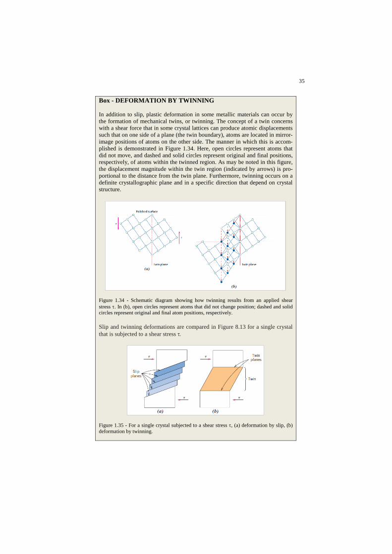
Box - DEFORMATION BY TWINNING In addition to slip, plastic deformation in some metallic materials can occur by the formation of mechanical twins, or twinning. The concept of a twin concerns with a shear force that in some crystal lattices can produce atomic displacements such that on one side of a plane (the twin boundary), atoms are located in mirror-image positions of atoms on the other side. The manner in which this is accom-plished is demonstrated in Figure 1.34. Here, open circles represent atoms that did not move, and dashed and solid circles represent original and final positions, respectively, of atoms within the twinned region. As may be noted in this figure, the displacement magnitude within the twin region (indicated by arrows) is pro-portional to the distance from the twin plane. Furthermore, twinning occurs on a definite crystallographic plane and in a specific direction that depend on crystal structure.

Figure 1.34 - Schematic diagram showing how twinning results from an applied shear stress τ. In (b), open circles represent atoms that did not change position; dashed and solid circles represent original and final atom positions, respectively.

Slip and twinning deformations are compared in Figure 8.13 for a single crystal that is subjected to a shear stress τ.

Figure 1.35 - For a single crystal subjected to a shear stress τ, (a) deformation by slip, (b) deformation by twinning.

36

Mechanical twinning occurs in metals that have BCC and HCP crystal structures, at low temperatures, and at high rates of loading (shock loading), conditions un-der which the slip process is restricted; that is, there are few operable slip sys-tems.

Mechanisms of Strengthening in Metals

Metallurgical and materials engineers are often called on to design alloys having high strengths yet some ductility and toughness; typically, ductility is sacrificed when an alloy is strengthened. Several hardening techniques are at the disposal of an engineer, and frequently alloy selection depends on the capacity of a material to be tailored with the mechanical characteristics required for a particular applica-tion. Important to the understanding of strengthening mechanisms is the relation between dislocation motion and mechanical behavior of metals. Because macro-scopic plastic deformation corresponds to the motion of large numbers of disloca-tions, the ability of a metal to deform plastically depends on the ability of disloca-tions to move. Because hardness and strength (both yield and tensile) are related to the ease with which plastic deformation can be made to occur, by reducing the mobility of dislocations, the mechanical strength may be enhanced; that is, greater mechanical forces will be required to initiate plastic deformation. In contrast, the more unconstrained the dislocation motion, the greater is the facility with which a metal may deform, and the softer and weaker it becomes. Virtually all strengthen-ing techniques rely on this simple principle: Restricting or hindering dislocation motion renders a material harder and stronger. The present discussion is confined to strengthening mechanisms for single-phase metals by grain size reduction, sol-id-solution alloying, and strain hardening. Deformation and strengthening of mul-tiphase alloys are more complicated, involving concepts beyond the scope of the present discussion; later chapters treat techniques that are used to strengthen mul-tiphase alloys.

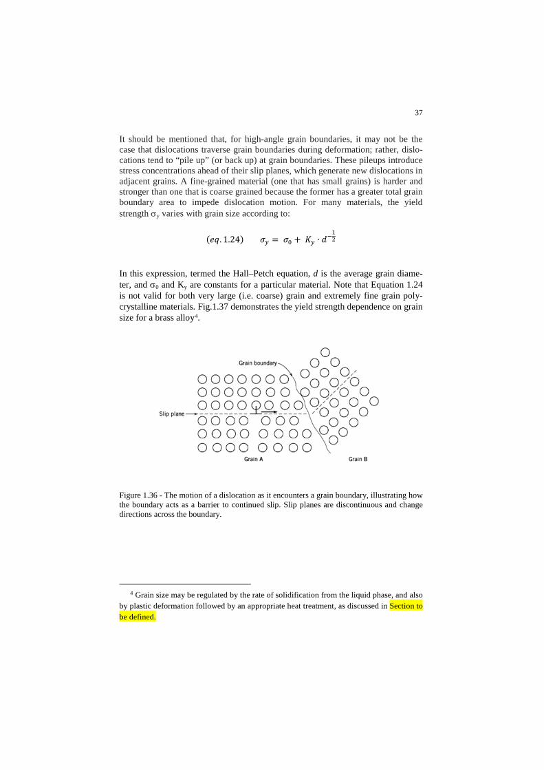
Strengthening by grain size reduction The size of the grains, or average grain diameter, in a polycrystalline metal influ-ences the mechanical properties. Adjacent grains normally have different crystal-lographic orientations and, of course, a common grain boundary, as indicated in Fig. 1.36. During plastic deformation, slip or dislocation motion must take place across this common boundary— say, from grain A to grain B in Fig.1.36.The grain boundary acts as a barrier to dislocation motion for two reasons:

1. Because the two grains are of different orientations, a dislocation passing into grain B will have to change its direction of motion; this becomes more difficult as the crystallographic misorientation increases.

2. The atomic disorder within a grain boundary region will result in a dis-continuity of slip planes from one grain into the other.

37

It should be mentioned that, for high-angle grain boundaries, it may not be the case that dislocations traverse grain boundaries during deformation; rather, dislo-cations tend to “pile up” (or back up) at grain boundaries. These pileups introduce stress concentrations ahead of their slip planes, which generate new dislocations in adjacent grains. A fine-grained material (one that has small grains) is harder and stronger than one that is coarse grained because the former has a greater total grain boundary area to impede dislocation motion. For many materials, the yield strength σy varies with grain size according to:

(𝑒𝑒𝑒𝑒. 1.24) 𝜎𝜎𝑦𝑦 = 𝜎𝜎0 + 𝐾𝐾𝑦𝑦 ∙ 𝑑𝑑−12

In this expression, termed the Hall–Petch equation, d is the average grain diame-ter, and σ0 and Ky are constants for a particular material. Note that Equation 1.24 is not valid for both very large (i.e. coarse) grain and extremely fine grain poly-crystalline materials. Fig.1.37 demonstrates the yield strength dependence on grain size for a brass alloy4.

Figure 1.36 - The motion of a dislocation as it encounters a grain boundary, illustrating how the boundary acts as a barrier to continued slip. Slip planes are discontinuous and change directions across the boundary.

4 Grain size may be regulated by the rate of solidification from the liquid phase, and also by plastic deformation followed by an appropriate heat treatment, as discussed in Section to be defined.

38

Figure 1.37 - The influence of grain size on the yield strength of a 70 Cu–30 Zn brass alloy. Note that the grain diameter increases from right to left and is not linear. It should also be mentioned that grain size reduction improves not only the strength, but also the toughness of many alloys; this fact can be explained as fol-lows. Considering the scheme in Fig.1.31, if you imagine to reduce the grain size, many grains will “appear” in the same round window. This fact implies several further slip systems will add, because they are pertinent to each single new grain you may consider. The result is the following. On one hand increasing of number of grain boundaries, that leads to increasing strength as above discussed; on the other hand, the increasing number of slip systems can contemporarily lead materi-al to be prone dislocation movement inside the grain; this phenomenon results in higher energy “absorption” during dislocation movement inside the grain, toward the grain boundaries where dislocation will pile up. Small-angle grain boundaries are not effective in interfering with the slip process because of the slight crystallographic misalignment across the boundary. On the other hand, twin boundaries will effectively block slip and increase the strength of the material. Boundaries between two different phases are also impediments to movements of dislocations; this is important in the strengthening of more complex alloys.

39

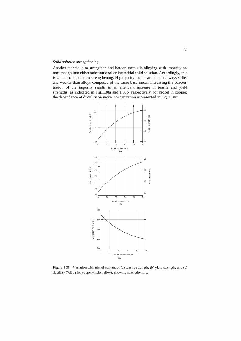
Solid solution strengthening Another technique to strengthen and harden metals is alloying with impurity at-oms that go into either substitutional or interstitial solid solution. Accordingly, this is called solid solution strengthening. High-purity metals are almost always softer and weaker than alloys composed of the same base metal. Increasing the concen-tration of the impurity results in an attendant increase in tensile and yield strengths, as indicated in Fig.1.38a and 1.38b, respectively, for nickel in copper; the dependence of ductility on nickel concentration is presented in Fig. 1.38c.

Figure 1.38 - Variation with nickel content of (a) tensile strength, (b) yield strength, and (c) ductility (%EL) for copper–nickel alloys, showing strengthening.

40

Alloys are stronger than pure metals because impurity atoms that go into solid so-lution typically impose lattice strains on the surrounding host atoms. Lattice strain field interactions between dislocations and these impurity atoms result, and, con-sequently, dislocation movement is restricted. For example, an impurity atom that is smaller than a host atom for which it substitutes exerts tensile strains on the sur-rounding crystal lattice, as illustrated in Figure 1.39a.

Figure 1.39 - (a) Representation of tensile lattice strains imposed on host atoms by a small-er substitutional impurity atom. (b) Possible locations of smaller impurity atoms relative to an edge dislocation such that there is partial cancellation of impurity–dislocation lattice strains.

Figure 1.40 - (a) Representation of compressive strains imposed on host atoms by a larger substitutional impurity atom. (b) Possible locations of larger impurity atoms relative to an edge dislocation such that there is partial cancellation of impurity–dislocation lattice strains. Conversely, a larger substitutional atom imposes compressive strains in its vicinity (Figure 1.40a).These solute atoms tend to diffuse to and segregate around disloca-tions in such a way as to reduce the overall strain energy—that is, to cancel some of the strain in the lattice surrounding a dislocation. To accomplish this, a smaller impurity atom is located where its tensile strain will partially nullify some of the dislocation’s compressive strain. For the edge dislocation in Figure 1.39b, this would be adjacent to the dislocation line and above the slip plane. A larger impuri-

41

ty atom would be situated as in Figure 1.40b. The resistance to slip is greater when impurity atoms are present because the overall lattice strain must increase if a dis-location is torn away from them. Furthermore, the same lattice strain interactions (Figures 1.39b and 1.40b) will exist between impurity atoms and dislocations that are in motion during plastic deformation. Thus, a greater applied stress is neces-sary to first initiate and then continue plastic deformation for solid-solution alloys, as opposed to pure metals; this is evidenced by the enhancement of strength and hardness. Strain hardening Strain hardening is the phenomenon by which a ductile metal becomes harder and stronger as it is plastically deformed. Sometimes it is also called work hardening or, because the temperature at which deformation takes place is “cold” relative to the absolute melting temperature of the metal, cold working. Most metals strain harden at room temperature. Fig. 1.41a and 1.41b demonstrate how steel, brass, and copper increase in yield and tensile strength with increasing cold work. The price for this enhancement of hardness and strength is in a decrease in the ductility of the metal. This is shown in Fig.1.41c, in which the ductility, in percent elonga-tion, experiences a reduction with increasing percent cold work for the same three alloys.

Figure 1.41 - For 1040 steel, brass, and copper, (a) the increase in yield strength, (b) the increase in tensile strength, and (c) the decrease in ductility (%EL) with percent cold work The influence of cold work on the stress–strain behavior of a low-carbon steel is shown in Figure 8.20; here stress–strain curves are plotted at 0%CW, 4%CW, and 24%CW.

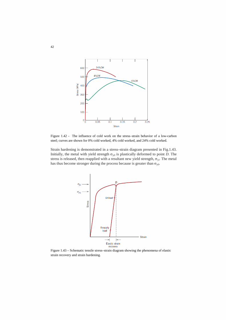
42

Figure 1.42 - The influence of cold work on the stress–strain behavior of a low-carbon steel; curves are shown for 0% cold worked, 4% cold worked, and 24% cold worked. Strain hardening is demonstrated in a stress–strain diagram presented in Fig.1.43. Initially, the metal with yield strength σy0 is plastically deformed to point D. The stress is released, then reapplied with a resultant new yield strength, σyi. The metal has thus become stronger during the process because is greater than σy0.

Figure 1.43 – Schematic tensile stress–strain diagram showing the phenomena of elastic strain recovery and strain hardening.

43

The strain-hardening phenomenon is explained on the basis of dislocation– dislo-cation strain field interactions similar to those discussed for the solid solution strengthening, but more effective. The dislocation density in a metal increases with deformation or cold work because of dislocation multiplication or the for-mation of new dislocations, as noted previously. Consequently, the average dis-tance of separation between dislocations decreases—the dislocations are posi-tioned closer together. On the average, dislocation–dislocation strain interactions are repulsive. The net result is that the motion of a dislocation is hindered by the presence of other dislocations. As the dislocation density increases, this resistance to dislocation motion by other dislocations becomes more pronounced. As a metal is plastically deformed, new dislocations are thus created, so that the dislocation density becomes higher and higher. In addition to multiplying, the dis-locations become entangled and impede each others’ motion. Dislocations, in fact, are influenced by the presence of other dislocations and interact with each other, as shown for a number of different interactions in Fig. 1.44.

Figure 1.44 – Examples of dislocation interactions. Dislocations of the same sign will repel each other, while dislocations of opposite signs will attract each other and, if they meet, annihilate each other. If the two dis-locations of opposite signs are not on the same slip plane, they will merge to form a row of vacancies. These types of interactions occur because they reduce the in-ternal energy of the system. The result, in any case, is increasing resistance to plastic deformation with increas-ing dislocation density. Work hardening thus results in a simultaneous increase in strength and a decrease in ductility. Since the work hardened condition increases

44

the stored energy in the metal and is thermodynamically unstable, the deformed metal will try to return to a state of lower energy. This generally cannot be accom-plished at room temperature. Elevated temperatures, in the range of 1/2 to 3/4 of the absolute melting point, are necessary to allow mechanisms, such as diffusion, to restore the lower-energy state. The process of heating a work-hardened metal to restore its original strength and ductility is called annealing. Metals undergoing forming operations often require intermediate anneals to restore enough ductility to continue the forming operation. Approximately 5% of the energy of defor-mation is retained internally as dislocations when a metal is plastically deformed, while the rest is dissipated as heat. The imposed stress necessary to deform a metal increases with increasing cold work. In the mathematical expression relating true stress and strain shown by equation 1.25:

(𝑒𝑒𝑒𝑒. 1.25) 𝜎𝜎 = 𝐾𝐾 ∙ 𝜀𝜀𝑛𝑛 the parameter n is called the strain-hardening exponent, which is a measure of the ability of a metal to strain harden; the larger its magnitude, the greater is the strain hardening for a given amount of plastic strain. Phase boundaries as strengthening sources While a grain boundary is an interface between grains of the same composition and same crystalline structure (α/α interface) with different orientations, a phase boundary is one between two different phases (α/β interface) that can have differ-ent crystalline structures and/or different compositions. In two-phase alloys, such as copper-zinc brass alloys containing more than 40% Zn, second phases, such as the one shown in Fig. 1.45, can form due to the limited solid solubility of zinc in copper.

Figure 1.45 – Phase boundary in copper-zinc system.

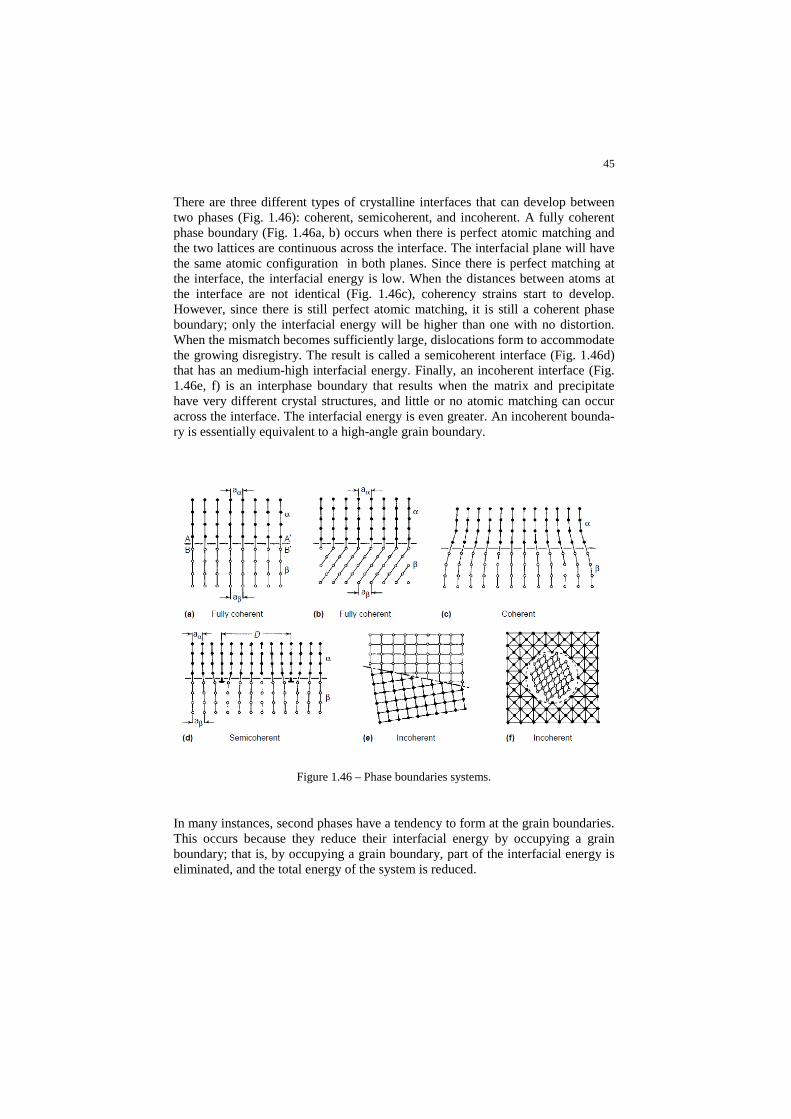
45

There are three different types of crystalline interfaces that can develop between two phases (Fig. 1.46): coherent, semicoherent, and incoherent. A fully coherent phase boundary (Fig. 1.46a, b) occurs when there is perfect atomic matching and the two lattices are continuous across the interface. The interfacial plane will have the same atomic configuration in both planes. Since there is perfect matching at the interface, the interfacial energy is low. When the distances between atoms at the interface are not identical (Fig. 1.46c), coherency strains start to develop. However, since there is still perfect atomic matching, it is still a coherent phase boundary; only the interfacial energy will be higher than one with no distortion. When the mismatch becomes sufficiently large, dislocations form to accommodate the growing disregistry. The result is called a semicoherent interface (Fig. 1.46d) that has an medium-high interfacial energy. Finally, an incoherent interface (Fig. 1.46e, f) is an interphase boundary that results when the matrix and precipitate have very different crystal structures, and little or no atomic matching can occur across the interface. The interfacial energy is even greater. An incoherent bounda-ry is essentially equivalent to a high-angle grain boundary.

Figure 1.46 – Phase boundaries systems. In many instances, second phases have a tendency to form at the grain boundaries. This occurs because they reduce their interfacial energy by occupying a grain boundary; that is, by occupying a grain boundary, part of the interfacial energy is eliminated, and the total energy of the system is reduced.

46

Depending on the type of their phase boundaries, such fine particles can exhibit slight or very high obstruction to dislocation movement. These in fact are in any case an irregularity for the matrix crystal lattice constituting the grain where dislo-cation can move. These fine precipitate particles, in other words, act as barriers to the motion of dislocations and provide resistance to slip, thereby increasing the strength and hardness. Particles are usually classified as deformable or non-deformable, meaning that the dislocation is able to cut through it (deformable) or the particle is so strong that the dislocation cannot cut through (non-deformable). When a dislocation encoun-ters a fine particle, it must either cut through the particle or bow (loop) around it, as shown schematically in Fig. 1.47.

Figure 1.47 – Particle strengthening. For effective particle strengthening (Fig. 1.48), the matrix should be soft and duc-tile, while the particles should be hard and discontinuous. A ductile matrix is bet-ter in resisting catastrophic crack propagation. Smaller and more numerous parti-cles are more effective at interfering with dislocation motion than larger and more widely spaced particles. Preferably, the particles should be spherical rather than needlelike to prevent stress-concentration effects. Finally, larger amounts of parti-cles increase strengthening.

47

Figure 1.48 – Particle-hardening considerations. In summary we have discussed mechanisms that may be used to strengthen and harden single-phase metal alloys: strengthening by grain size reduction, solid-solution strengthening, strain hardening and second phase-dispersed (or fine parti-cles) hardening. Of course they may be used in conjunction with one another; for example, a solid-solution-strengthened alloy may also be strain hardened.

Grain Growth, Recovery and Recrystallization Plastically deforming a polycrystalline metal specimen at temperatures that are low relative to its absolute melting temperature produces microstructural and property changes that include (1) a change in grain shape, (2) strain hardening, and (3) an in-crease in dislocation density. Some fraction of the energy expended in deformation is stored in the metal as strain energy, which is associated with tensile, compressive, and shear zones around the newly created dislocations. These properties and structures may revert back to the pre–cold-worked states by ap-propriate heat treatment, sometimes termed an annealing treatment. Such restoration results from two different processes that occur at elevated temperatures: recovery and recrystallization, which may be followed by grain growth. Recovery Recovery is the initial stage of the annealing cycle before recrystallization occurs. During recovery, some of the stored internal strain energy is relieved by virtue of dislocation motion (in the absence of an externally applied stress), as a result of enhanced atomic diffusion at the elevated temperature. There is some reduction in

48

the number of dislocations, and dislocation configurations are produced having low strain energies. During recovery, basic types of processes that occur are:

(1) the annihilation of excess point defects, particularly vacancies; the va-cancies that were generated during cold working are annealed out by mi-grating to dislocations, grain boundaries, or surfaces;

(2) the rearrangement of dislocations into lower energy configurations, which also annihilates many of them; At slightly higher temperatures, the rearrangement of dislocations occurs, and, in the process, the annihilation of dislocations of opposite signs takes place. The rearrangement of dislo-cations is assisted by thermal energy, which aids in both climb and slip mechanisms.

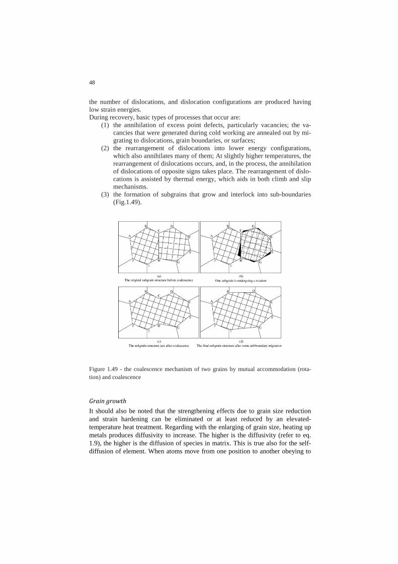
(3) the formation of subgrains that grow and interlock into sub-boundaries (Fig.1.49).

Figure 1.49 - the coalescence mechanism of two grains by mutual accommodation (rota-tion) and coalescence Grain growth It should also be noted that the strengthening effects due to grain size reduction and strain hardening can be eliminated or at least reduced by an elevated-temperature heat treatment. Regarding with the enlarging of grain size, heating up metals produces diffusivity to increase. The higher is the diffusivity (refer to eq. 1.9), the higher is the diffusion of species in matrix. This is true also for the self-diffusion of element. When atoms move from one position to another obeying to

49

diffusion mechanisms (refer to par.” Vacancies, interstitial spaces and grain boundaries as drive-force for diffusion in metals”), they also can move from one grain boundary to another: what could happen is schematically shown in Fig.1.50a. Basing on the grain boundary “migration”, in the Fig. 1.50b is shown the mechanisms that provokes grain growth by small grains disappearing. Ulti-mately, grain growth occurs because of metal with its original microstructure is heated up to certain temperature (Fig.1.51).

(a)

(b)

Figure 1.50 – (a) Schematic representation of grain growth via atomic diffusion; (b) disap-pearing of small grains. Empirically, it has been shown that grain growth occurs according to: (𝑒𝑒𝑒𝑒. 1.26) 𝐷𝐷 = 𝐾𝐾 ∙ 𝑡𝑡𝑛𝑛 Where: D is the average grain diameter, t is time, n is a constant,

𝐾𝐾 = 𝐾𝐾0 ∙ 𝑒𝑒− 𝑄𝑄2𝑅𝑅𝑅𝑅

50

The constant n increases with temperature and approaches a theoretical value of 0.5. It should also be noted that the activation energy, Q, also varies with tempera-ture.

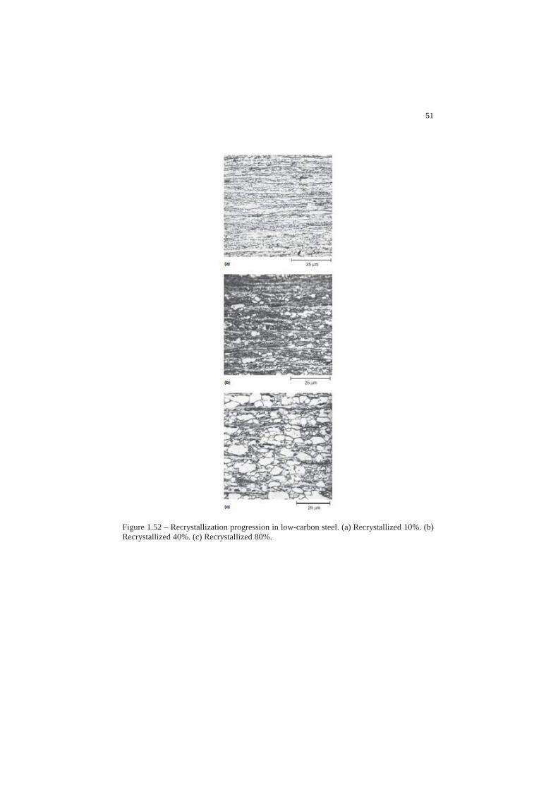
Figure 1.51 – Schematic representation of grain size versus treatment temperature relation-ship. Recrystallization Even after recovery is complete, the grains are still in a relatively high strain ener-gy state. Recrystallization is the formation of a new set of strain-free and equiaxed grains (i.e., having approximately equal dimensions in all directions) that have low dislocation densities and are characteristic of the pre–cold-worked condition. The driving force to produce this new grain structure is the difference in internal ener-gy between the strained and unstrained material. The new grains form as very small nuclei and grow until they completely consume the parent material, process-es that involve short range diffusion. Two stages in the recrystallization process are represented in Fig.1.52a, 1.52b and 1.52c. In these photomicrographs, the small, speckled grains are those that have recrystallized. Recrystallization of cold-worked metals may be used to refine the grain structure. Also, during recrystallization, the mechanical properties that were changed as a result of cold working are restored to their pre–cold-worked values; that is, the metal becomes softer and weaker, yet more ductile (the extent of recrystallization depends on both time and temperature), as shown in Fig.1.53. The influence of temperature is demonstrated in Figure 1.54, which plots tensile strength and ductility (at room temperature) of a brass alloy as a function of the temperature and for a constant heat treatment time of 1 h. The grain structures found at the various stages of the process are also presented schematically. Recrystallization is considered complete when the mechanical properties of the re-crystallized metal approach those of the metal before it was cold worked; on the other hand, recrystallization and the resulting mechanical softening completely cancel the effects of cold working.

51

Figure 1.52 – Recrystallization progression in low-carbon steel. (a) Recrystallized 10%. (b) Recrystallized 40%. (c) Recrystallized 80%.

52

Figure 1.53 – The influence of annealing temperature (for an annealing time of 1 h) on the tensile strength and ductility of a brass alloy. Grain size as a function of annealing tempera-ture is indicated. Grain structures during recovery, recrystallization, and grain growth stag-es are shown schematically.

Figure 1.54 – The variation of recrystallization temperature with percent cold work for iron. For deformations less than the critical (about 5% cold work, CW), recrystallization will not occur.

53

Plastic deformation operations are often carried out at temperatures above the recrys-tallization temperature in a process termed hot working (Fig.1.55), described in Sec-tion to be defined. The material remains relatively soft and ductile during deformation because it does not strain harden, and thus large deformations are possible.

Figure 1.55 – Recrystallization during hot rolling.

Mechanical behavior of metals by macroscopic approach

The mechanical behavior of a material is its response to an applied load or force. Important mechanical properties are strength, hardness, stiffness, and ductility. There are three principal ways in which a load may be applied: tension, compres-sion, and shear. Large number of mechanical property tests have been developed to determine a material response to applied loads or forces. Tensile test The tensile test is the most commonly used mechanical property test. Its chief use is to determine the properties related to the elastic design of structures. In addition, the tensile test gives information on the plasticity and fracture of a material. A typ-ical stress-strain curve for a metal is shown in Fig. 1.55. The parameters used to describe the stress-strain curve of a metal are the tensile strength, yield strength or yield point, percent elongation, and reduction in area. The first two are strength parameters, and the last two are indications of ductility. As long as the specimen is loaded within the elastic region, the strain is totally recoverable. However, when the load exceeds a value to the yield stress, the specimen undergoes plastic de-formation and is permanently deformed when the load is removed. The stress to produce continued plastic deformation increases with increasing strain, thus obey-ing to work hardening phenomenon, discussed above as one of strengthening mechanism active in metals. To a good engineering approximation, the volume remains constant during plastic deformation (Al=A0l0), and as the specimen elon-gates, it decreases uniformly in cross-sectional area along its gage length. Initially,

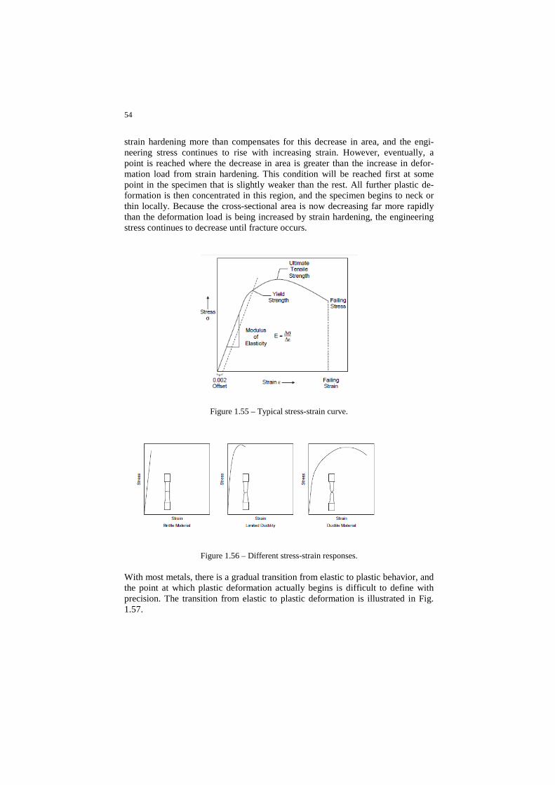
54

strain hardening more than compensates for this decrease in area, and the engi-neering stress continues to rise with increasing strain. However, eventually, a point is reached where the decrease in area is greater than the increase in defor-mation load from strain hardening. This condition will be reached first at some point in the specimen that is slightly weaker than the rest. All further plastic de-formation is then concentrated in this region, and the specimen begins to neck or thin locally. Because the cross-sectional area is now decreasing far more rapidly than the deformation load is being increased by strain hardening, the engineering stress continues to decrease until fracture occurs.

Figure 1.55 – Typical stress-strain curve.

Figure 1.56 – Different stress-strain responses. With most metals, there is a gradual transition from elastic to plastic behavior, and the point at which plastic deformation actually begins is difficult to define with precision. The transition from elastic to plastic deformation is illustrated in Fig. 1.57.

55

Figure 1.57 – Elastic and plastic behavior during tensile loading. Metals that yield discontinuously have a stress-strain curve similar to that shown in Fig. 1.58a, instead of a continuous gradual yield point as in Fig. 1.58b. While in the former case the yield point is univocally identified as lower and higher yield point (see Fig.1.58a), for the metals with indefinite yield point, yield strength is determined by drawing a straight line parallel to the initial straight line portion of the stress-strain curve. The line is normally offset by a strain of 0.2% (0.002).

(a) (b)

Figure 1.58– (a) Transition from elastic to plastic behavior; (b) Discontinuous yielding in plain carbon steels.

56

Ductility Measures of ductility that are obtained from the tension test are the engineering strain at fracture (εf) and the reduction of area at fracture. Both are usually ex-pressed as percentages, with the engineering strain at failure often reported as the percent elongation. Both of these properties are obtained after fracture by putting the specimen back together and taking measurements of the final length, lf, and fi-nal specimen cross section at fracture, Af. Percent elongation can be determined by:

where l0 is the original gage length, and lf is the final length of the gage section. Likewise, reduction in area can be determined by:

where A0 is the original area of the gage section, and Af is the final area of the gage section at fracture. Resilience Resilience is the capacity of a material to absorb energy when it is deformed elas-tically and then, upon unloading, to have this energy recovered. The associated property is the modulus of resilience, Ur , which is the strain energy per unit vol-ume required to stress a material from an unloaded state up to the point of yield-ing. The modulus of resilience for a specimen subjected to a uniaxial tension test is just the area under the engineering stress–strain curve taken to yielding:

(𝑒𝑒𝑒𝑒. 1.27) 𝑈𝑈𝑐𝑐 = � 𝜎𝜎𝑑𝑑𝜀𝜀𝜀𝜀𝑦𝑦

0

Assuming a linear elastic region, we have:

(𝑒𝑒𝑒𝑒. 1.28) 𝑈𝑈𝑐𝑐 =12𝜎𝜎𝑦𝑦𝜀𝜀𝑦𝑦 = [𝑠𝑠𝑠𝑠𝑠𝑠𝑠𝑠𝑡𝑡𝑐𝑐𝑡𝑡𝑠𝑠𝑡𝑡𝑐𝑐𝑐𝑐𝑔𝑔 𝑡𝑡ℎ𝑒𝑒 𝐻𝐻𝑐𝑐𝑐𝑐𝐻𝐻 𝐿𝐿𝑐𝑐𝐿𝐿 ] =

12𝜎𝜎𝑦𝑦2

𝐸𝐸

in which εy is the strain at yielding (see scheme in Fig.1.59). The units of resilience are the product of the units from each of the two axes of the stress–strain plot. For SI units, this is joules per cubic meter (J/m3, equivalent to Pa).

57

Figure 1.59– Schematic representation showing how modulus of resilience (corresponding to the shaded area) is determined from the tensile stress–strain behavior of a material. Toughness Although there are a number of approaches to defining toughness, one of the old-est is to consider it as the total area under the stress-strain curve. This area is an indication of the amount of work per unit volume that can be done on a material without causing it to fail. As shown in Fig. 1.60, this definition of toughness im-plies that toughness is a function of both strength and ductility. Another way of defining toughness is as the ability of a material to absorb energy and plastically deform before fracturing. For dynamic (high strain rate) loading conditions and when a notch (or point of stress concentration) is present, notch toughness is assessed by using an impact test (Fig.1.61).

Figure 1.60 – Area under stress-strain curve as a measure of toughness.

58

Figure 1.61 – Impact test machine (Charpy test) conducted onto notched specimen.

Box – Stress concentration Geometrical features, such as holes, fillets, and radii, produce higher local stresses than encountered in the body of the material. For example, the tensile stresses at the top and bottom of the hole shown in Fig. 1.62 are three times greater than they are in the body of the material. These higher stresses are a result of the inability of the stresses to pass through the hole.

Figure 1.62 – Stress-concentration effect around a hole. Such stress increases are described by the stress-concentration factor, K: K = Maximum actual stress/ Nominal stress While the stress-concentration factor K for a round hole is 3, much higher stress concentration factors occur when there is a sharp notch in the material. Values for a wide range of geometries can be found in handbooks dealing with stress analysis.

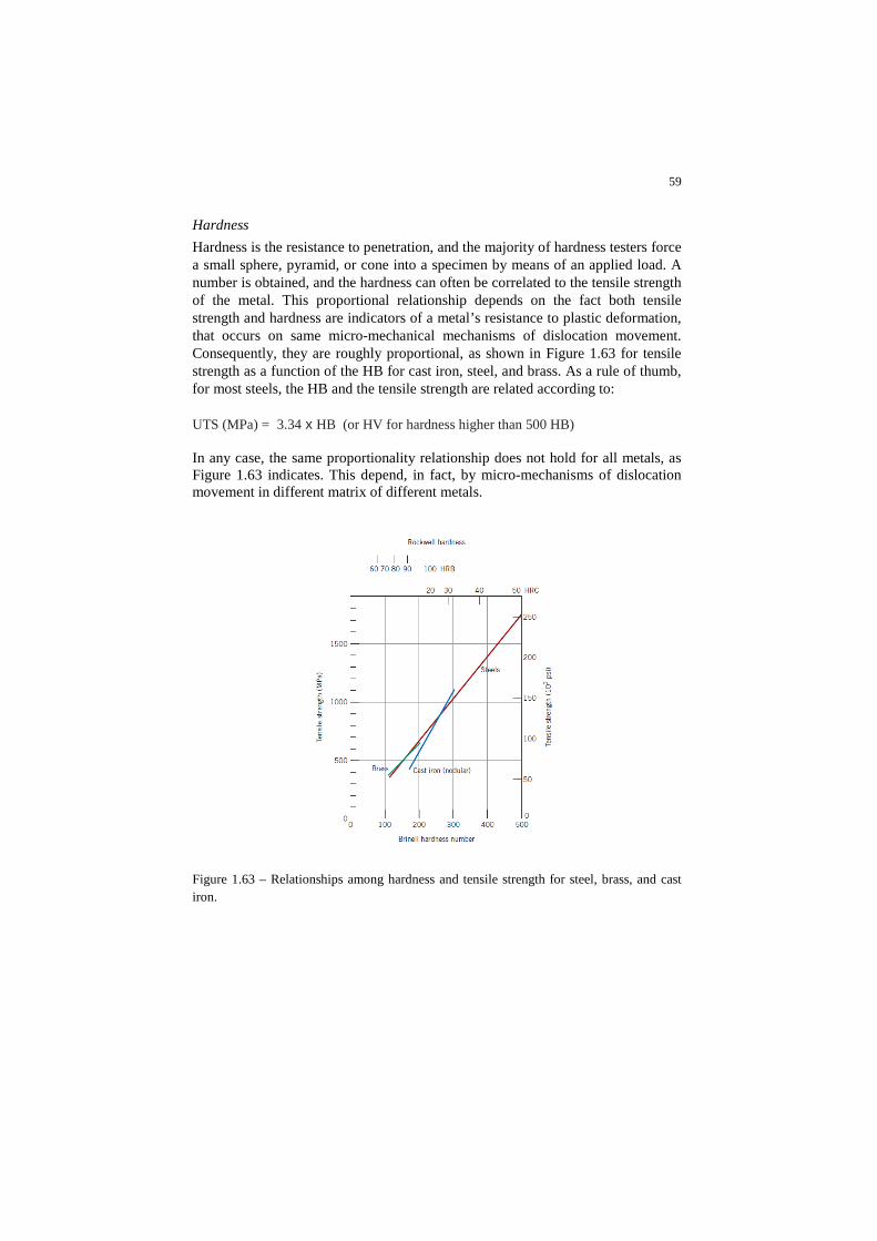
59

Hardness Hardness is the resistance to penetration, and the majority of hardness testers force a small sphere, pyramid, or cone into a specimen by means of an applied load. A number is obtained, and the hardness can often be correlated to the tensile strength of the metal. This proportional relationship depends on the fact both tensile strength and hardness are indicators of a metal’s resistance to plastic deformation, that occurs on same micro-mechanical mechanisms of dislocation movement. Consequently, they are roughly proportional, as shown in Figure 1.63 for tensile strength as a function of the HB for cast iron, steel, and brass. As a rule of thumb, for most steels, the HB and the tensile strength are related according to:

UTS (MPa) = 3.34 x HB (or HV for hardness higher than 500 HB) In any case, the same proportionality relationship does not hold for all metals, as Figure 1.63 indicates. This depend, in fact, by micro-mechanisms of dislocation movement in different matrix of different metals.

Figure 1.63 – Relationships among hardness and tensile strength for steel, brass, and cast iron.

60

Box – Hardness test, the basics.

Resuming the main contents, defining the main paradigm for mechanical response of metals

On an atomic scale level, plastic deformation corresponds to the motion of dislo-cations in response to an externally applied shear stress. For example, an edge dis-location moves by the successive and repeated breaking of atomic bonds and shift-ing by interatomic distances of half planes of atoms. For dislocation edge, in particular, dislocation line motion and direction of the applied shear stress are thus parallel. We call slip the motion of dislocations in response to an externally ap-plied shear stress. It occurs on specific crystallographic planes and within these planes only in certain directions, depending on crystal structure of the metal. The combination of slip planes and slip direction, expressed by the Schmid’s Law, is defined slip system. The slip plane is that plane that has the densest atomic pack-ing, and the slip direction is the direction within this plane that is most closely packed with atoms. Operable slip systems, namely the planes where dislocation are active, depend on the crystal structure of the material. A resolved shear stress is the shear stress resulting from an applied tensile stress that is resolved onto a plane that is neither parallel nor perpendicular to the stress direction. For polycrystalline materials, slip occurs within each grain along those slip systems that are most favorably oriented with the applied stress. As favorable

61

oriented we mean that in such grains the resolved shear stress is highest and it can achieve the critical shear stress, namely the shear stress necessary to activate dis-location slip along slip plane and in the slip direction. During deformation, grains change shape and extend in those directions wherein there is gross plastic defor-mation. The basic concept is that the ease with which a material is capable of plastic de-formation is a function of dislocation mobility—that is, restricting dislocation mo-tion leads to increases hardness and strength. Various modes are practicable to inhibit dislocation mobility. We call these modes strengthening mechanisms:

- Grain Size Reduction: as grain boundaries are barriers to dislocation motion for two reasons: a) when crossing a grain boundary, a disloca-tion’s direction of motion must change; b) there is a discontinuity of slip planes within the vicinity of a grain boundary. A metal that has small grains will be stronger than one with large grains because the former has more grain boundary area, and, thus, more barriers to dislocation motion. For most metals, yield strength depends on average grain diameter ac-cording to the Hall–Petch equation.

- Solid-Solution Strengthening: the strength and hardness of a metal in-crease with increase of concentration of impurity atoms that go into solid solution (both substitutional and interstitial).Solid-solution strengthening results from lattice strain interactions between impurity atoms and dislo-cations; these interactions produce a diminishment in dislocation mobili-ty.

- Strain Hardening: strain hardening is just the enhancement in strength (and decrease of ductility)of a metal as it is plastically deformed. Degree of plastic deformation may be expressed as percent cold work, which de-pends on original and deformed cross-sectional areas. Yield strength, ten-sile strength, and hardness of a metal increase with increasing percent cold work; ductility diminishes. During plastic deformation dislocation density increases, the average distance between adjacent dislocations de-creases, and—because dislocation–dislocation strain field interactions, are, on average, repulsive—dislocation mobility becomes more restrict-ed; thus, the metal becomes harder and stronger.

On the opposite, mechanisms that tend to recover the dislocation mobility, driven by heating up structure, are:

- Recovery: There is some relief of internal strain energy by dislocation motion. Dislocation density decreases, and dislocations assume low-energy configurations. Some material properties revert back to their pre-cold-worked values.

- Recrystallization: During recrystallization, a new set of strain-free and equiaxed grains form that have relatively low dislocation densities. The metal becomes softer, weaker, and more ductile. The driving force for re-crystallization is the difference in internal energy between strained and recrystallized material. For a cold-worked metal that experiences recrys-tallization, as temperature increases (at constant heat-treating time), ten-

62

sile strength decreases and ductility. The recrystallization temperature of a metal alloy is that temperature at which recrystallization reaches com-pletion in one hour. Two factors that influence the recrystallization tem-perature are percent cold work and impurity content. Furthermore, re-crystallization temperature diminishes with increasing percent cold work.

- Grain growth is the increase in average grain size of polycrystalline ma-terials, which proceeds by grain boundary motion. The driving force for grain growth is the reduction in total grain boundary energy.

The most important conclusion we point out is the full understanding the strengthening mechanisms for metals and the resulting high or low mechanical properties on the microscopic scale is “easily” explained by a high or low disloca-tion motion resources. The higher is dislocation mobility, the lower is the onset to which plastic deformation occurs, namely the yield strength (YS) and the higher is the plastic deformation capacity under static or impacting loads that we expressed respectively by: a) the elongation percentage at break E% (alternatively or adding to % reduction of area at break) and b) the energy stored (i.e. the Joule absorbed) by breaking a standard notched sample by an impact test machine. Summarizing, we can quickly measure by tensile test and impact test some macro-scopic mechanical parameters by which we can state whether metallic materials behave either by ductile and tough safe mode or brittle unsafe mode. To under-stand why we can correlate the ductile and tough behavior to a safe operating mode of a metal for structural application, consider whether you would be happy to know the axle of your car is so low ductile and tough that its mechanical behav-ior is like a ceramic material. Basing on the 3 basic mechanical tests we have discussed so far, tensile test, hard-ness test and impact test, we therefore can group the main mechanical features we obtain by 3 type of tests, distinguishing in mechanical resistance properties and ductile properties, as shown in following Fig.1.65 Fig.1.65 – Basic mechanical properties from tensile test, hardness test and impact test grouped into: a) resistance capability (left side); b) ductility capability ( right side). As we already learned, the left side and right side properties for metal are strictly correlated, because of the following causal relationship:

i) Dislocations move and reach grain boundary grain boundary pe-rimeter modifies macroscopic plastic deformation occurs(1)

Hardness (hardness test) YS; UTS (tensile test)

E%, A% (tensile test) KV (Impact test, e.g. Charpy)

63

Note 1: For example macroscopic deformation is observed in surpassing the onset yield strength, necking occurs in tensile tests; indenting of test material by pene-trator in the hardness test; highly plastically deformed regions in the notched sec-tion area of Charpy test specimen broken.

And its own counteracting relationship :

ii) Dislocations are temporarily locked dislocation motion is inhibited critical resolved shear stress τcrss increases increase magnitude of external load to unlock dislocation(2) dislocation move and reach grain boundary…

Note 2: Refer to eq.1.22.

What happens in metals is that, as well as dislocations are inhibited in their movement (independently of reasons, namely whichever strengthening mechanism is established), the yield strength increases, the ultimate tensile strength increases, the hardness increases, as we expect because of the increase of such magnitude of external load capable to unlock dislocation; but at the same time, in strengthened matrix, mobility of dislocations decreases, thus resulting in decrease of ductile properties. The basic framework of such mutual relationships of a metal is shown in Fig.1.64.

Fig. 1.65 - Understanding basic material properties and their mutual correlations. For example, a high stiffness material (scheme on the left side) is a material with high slope – measured in the origin - of the σ (stress) and ε (deformation) curve obtained by a tensile test on the material. This slope is called the elastic modulus of the material. Such a high stiffness material usually exhibits further high mechanical strength (i.e. Ultimate Tensile Strength, UTS), low ductility (i.e. defor-mation at break, εr) and low toughness (i.e. energy stored to break, proportional to area below the σ−ε tensile test diagram).

σ

Strong, stiff and brittlematerial

High-tough and ductilematerial

Strong and low-toughmaterial

High toughness

High strength

Low strength

Low stiffness

High stiffness

Low toughness

ε

Low ductility high ductility

εr

UTSUTS

UTS

εr εr

64

For example, a high hardness and consequently lack of ductility of one phase found in steel, the martensite, is explained by a solid-solution strengthening effect, that leads to an increase of resolved critical shear stress and consequently external load necessary to unlock dislocations. But, in addition, the martensite structure has very few slip systems. These double conditions leads on one hand to a very high critical resolved shear stress, responsible of high hardness and the high strength of martensite; on the other hand very few possibilities offered to dislocation to move (few slip planes) causes few plastic deformation capability, that lead macroscopi-cally to very low ductility and toughness.

Microstructural Features of Fracture in Metallic Materials

The dislocation motion or their inhibition to movement plays a determinant role in the metal fracture. We mean as fracture in metals the same for any layman per-sons, not a metallurgist (actually you will be surprised in the following how much intuitive is the vocabulary of a metallurgist!). Thus, fracture is simply the separa-tion of a solid body made of metal into two or more pieces, under the action of ex-ternal load. For metals, fracture can be classified into two broad categories: a) ductile fracture and b) brittle fracture. The ductile or brittle mode depends primarily on the macro-scopic appearance of the fractured material. More precisely, the Fig. 13.1 shows a schematic comparison between two ductile fractures - on the right side – that are both characterized by extensive plastic deformation, prior to and during crack propagation.

Fig. 1.66 - Comparison of brittle and ductile fracture modes.

65

On the opposite, a brittle fracture occurs with little or no gross plastic deformation and usually occur suddenly, without warning (thus in unsafe mode - remind the ceramic vehicle axle!). The tendency for brittle fracture increases as well as any external or internal con-ditions work for: a) locking dislocations and/or b) reduce slip planes. Thus, the tendency for a material that has sufficient slip planes (this is not the case of the Hexagonal Close Packing crystal structure) to brittle behavior increases as well as its own dislocation population is inhibited in motion. This can happen, for exam-ple:

– with decreasing temperature; as temperature decreases, the atomic vibra-tion reduces and thus atomic planes tend to compact; this fact results unfa-vorable for dislocation slip;

– increasing strain rate, namely under strain-hardening mechanisms for dis-location locking;

– under triaxial stress conditions; remember that in the Mohr’s diagram a tri-axial tensile state of stress is represented by a point, not circles; in this spe-cial case, shear stresses are zero; no shear stress causes no dislocation slip can occur (refer to scheme in Fig.1.24);

In the following we go in depth in two modes as they appear to microscopic ob-servations. Ductile Fracture Ductile fracture normally occurs in a transgranular manner (through the grains) in metals that have good ductility and toughness. Often, a considerable amount of de-formation—including necking—is observed in the failed component.

Fig. 1.67 - When a ductile material is pulled in a tensile test, necking begins and voids form—starting near the center of the bar—by nucleation at grain boundaries or inclusions. As defor-mation continues, a 45° shear lip may form, producing a final cup and cone fracture.

66

The deformation occurs before the final fracture. Ductile fractures are usually caused by simple overloads, or by applying too high a stress to the material. In a simple tensile test, ductile fracture begins with the nucleation, growth, and coales-cence of microvoids near the center of the test bar (Figure 1.67). Microvoids form when a high stress causes separation of the metal at grain boundaries or interfaces between the metal and small impurity particles (inclusions). As the local stress in-creases, the microvoids grow and coalesce into larger cavities. Eventually, the metal-to-metal contact area is too small to support the load and fracture occurs. Deformation by slip also contributes to the ductile fracture of a metal. We know that slip occurs when the resolved shear stress reaches the critical resolved shear stress and that the resolved shear stresses are highest at a 45° angle to the applied tensile stress (ref. to Schmid’s Law). These two aspects of ductile fracture give the failed surface characteristic features. In thick metal sections, we expect to find evidence of necking, with a significant portion of the fracture surface having a flat face where microvoids first nucleated and coalesced, and a small shear lip, where the fracture surface is at a 45° angle to the applied stress. The shear lip, indicating that slip occurred, gives the fracture a cup and cone appearance (Figure 1.68).

Fig. 1.68 – Dimples form during ductile fracture. Equiaxed dimples form in the center, where microvoids grow. Elongated dimples, pointing toward the origin of failure, form on the shear lip. Simple macroscopic observation of this fracture may be sufficient to identify the ductile fracture mode. Examination of the fracture surface at a high magnifica-tion—perhaps using a scanning electron microscope—reveals a dimpled surface (Figure 1.69). The dimples are traces of the microvoids produced during fracture. Normally, these microvoids are round, or equiaxed, when a normal tensile stress produces the failure (see Figure 1.69a); however, on the shear lip, the dimples are oval-shaped, or elongated, with the ovals pointing toward the origin of the fracture (see Figure 1.69b).

67

Fig. 1.69 – Scanning electron micrographs of an annealed 1018 steel exhibiting ductile fracture in a tensile test. (a) Equiaxed dimples at the flat center of the cup and cone, and (b) elongated dimples at the shear lip. Brittle Fracture Brittle fracture occurs in high-strength metals and alloys or metals and alloys with poor ductility and toughness. Furthermore, even metals that are normally ductile may fail in a brittle manner at low temperatures, in thick sections, at high strain rates (such as impact), or when flaws play an important role. Brittle fractures are frequently observed when impact, rather than overload, causes failure. In brittle fracture, little or no plastic deformation is required. Initiation of the crack normal-ly occurs at small flaws, which cause a concentration of stress. The crack may move at a rate approaching the velocity of sound in the metal. Normally, the crack propagates most easily along specific crystallographic planes by cleavage. Cleavage fractures are characterized by a planar crack that changes planes by the formation of discrete steps. River patterns are formed at grain boundaries (Fig. 1.70) where the cleavage plane in one grain is not parallel to the plane in the adja-cent grain, the difference being accommodated by a series of steps. The river pat-terns eventually diminish as the crack propagates and adopts the cleavage plane of the new grain before being reformed at the next grain boundary. Brittle fracture can be identified by observing the features on the failed surface. Normally, the fracture surface is flat and perpendicular to the applied stress in a tensile test. If failure occurs by cleavage, each fractured grain is flat and different-ly oriented, giving a crystalline or “rock candy” appearance to the fracture surface (Fig. 1.71).

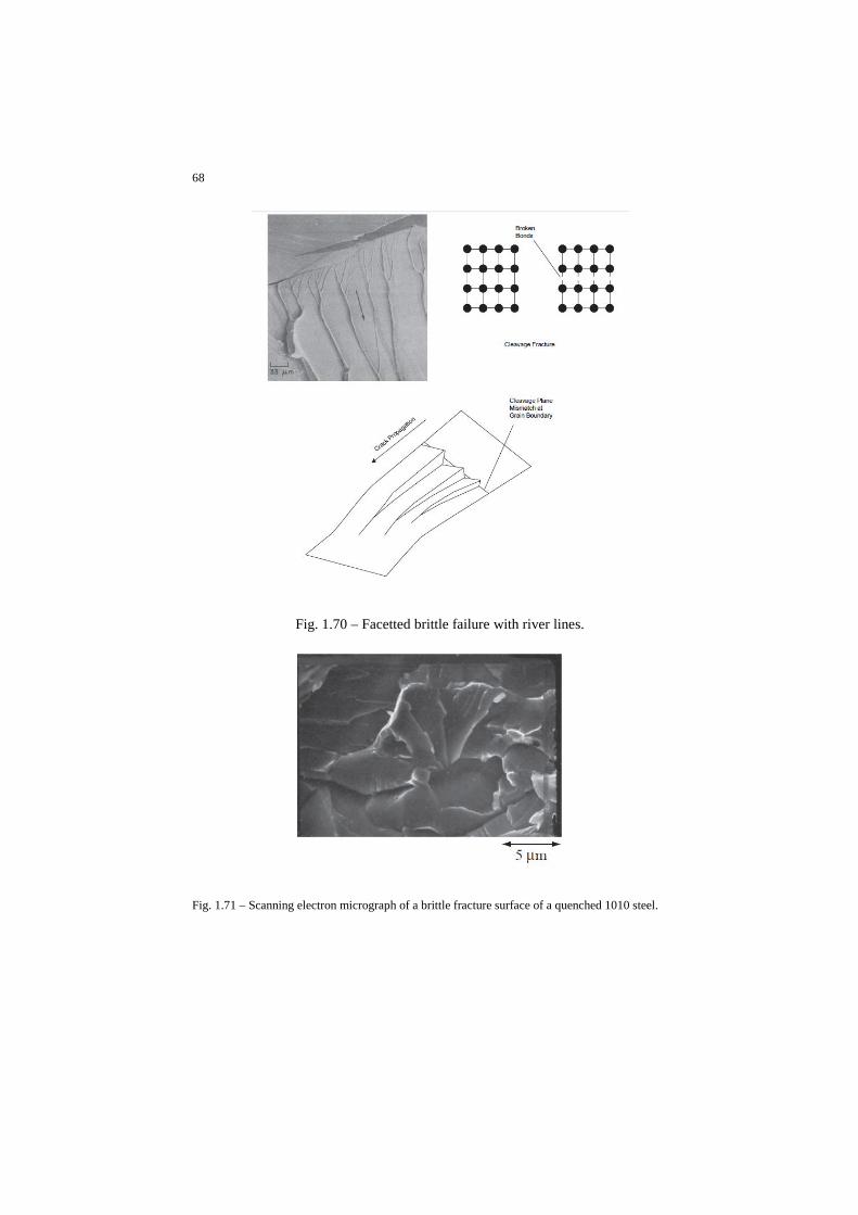
68

Fig. 1.70 – Facetted brittle failure with river lines.

Fig. 1.71 – Scanning electron micrograph of a brittle fracture surface of a quenched 1010 steel.

69

Another common fracture feature is the Chevron pattern (Figure 1.72), that ap-pears at naked eye. They are produced by separate crack fronts propagating at dif-ferent levels in the material. A radiating pattern of surface markings, or ridges, fans away from the origin of the crack (Figure 1.73). Since the Chevron pattern is visible with the naked eye or a magnifying glass and helps us identify both the brittle nature of the failure process as well as the origin of the failure. Actually we can say that the Chevron pattern are the naked eye result of the microscopic cleav-age fractures, thus observed at grain scale.

Fig. 1.72 – The Chevron pattern in quenched 4340 steel. The steel failed in a brittle manner by an impact blow

Fig. 1.73 – The Chevron pattern forms as the crack propagates from the origin at different levels. The pattern points back to the origin.

In some cases, however, the crack may take an intergranular (along the grain boundaries) path, when grain boundaries are abnormally weak (Fig.1.74).

70

Fig. 1.74 – The Chevron pattern forms as the crack propagates from the origin at different levels. The pattern points back to the origin.

Transgranular fracture(NORMAL )

Intergranular fracture(ABNORMAL )

71

In the next upload:

Chapter 2 - Damage mechanisms and root cause failure analysis basics

- Introduction

- Fast brittle fracture in metals

- Fatigue

- Creep and metal alloys for high temperature applica-

tions

- Wear

- Contact fatigue

- Corrosion