lecture notes in computer science 6744
TRANSCRIPT


Lecture Notes in Computer Science 6744Commenced Publication in 1973Founding and Former Series Editors:Gerhard Goos, Juris Hartmanis, and Jan van Leeuwen
Editorial Board
David HutchisonLancaster University, UK
Takeo KanadeCarnegie Mellon University, Pittsburgh, PA, USA
Josef KittlerUniversity of Surrey, Guildford, UK
Jon M. KleinbergCornell University, Ithaca, NY, USA
Alfred KobsaUniversity of California, Irvine, CA, USA
Friedemann MatternETH Zurich, Switzerland
John C. MitchellStanford University, CA, USA
Moni NaorWeizmann Institute of Science, Rehovot, Israel
Oscar NierstraszUniversity of Bern, Switzerland
C. Pandu RanganIndian Institute of Technology, Madras, India
Bernhard SteffenTU Dortmund University, Germany
Madhu SudanMicrosoft Research, Cambridge, MA, USA
Demetri TerzopoulosUniversity of California, Los Angeles, CA, USA
Doug TygarUniversity of California, Berkeley, CA, USA
Gerhard WeikumMax Planck Institute for Informatics, Saarbruecken, Germany


Sergei O. Kuznetsov Deba P. MandalMalay K. Kundu Sankar K. Pal (Eds.)
Pattern Recognitionand Machine Intelligence4th International Conference, PReMI 2011Moscow, Russia, June 27 – July 1, 2011Proceedings
13

Volume Editors
Sergei O. KuznetsovNational Research University Higher School of EconomicsSchool for Applied Mathematics and Information Science11 Pokrovski Boulevard, 109028 Moscow, RussiaE-mail: [email protected]
Deba P. MandalMalay K. KunduSankar K. PalIndian Statistical Institute, Machine Intelligence Unit203, B.T. Road, Kolkata 700108, IndiaE-mail: dpmandal, malay, [email protected]
ISSN 0302-9743 e-ISSN 1611-3349ISBN 978-3-642-21785-2 e-ISBN 978-3-642-21786-9DOI 10.1007/978-3-642-21786-9Springer Heidelberg Dordrecht London New York
Library of Congress Control Number: 2011929642
CR Subject Classification (1998): I.4, F.1, I.2, I.5, J.3, H.3-4, K.4.4, C.1.3
LNCS Sublibrary: SL 6 – Image Processing, Computer Vision, Pattern Recognition,and Graphics
© Springer-Verlag Berlin Heidelberg 2011This work is subject to copyright. All rights are reserved, whether the whole or part of the material isconcerned, specifically the rights of translation, reprinting, re-use of illustrations, recitation, broadcasting,reproduction on microfilms or in any other way, and storage in data banks. Duplication of this publicationor parts thereof is permitted only under the provisions of the German Copyright Law of September 9, 1965,in its current version, and permission for use must always be obtained from Springer. Violations are liableto prosecution under the German Copyright Law.The use of general descriptive names, registered names, trademarks, etc. in this publication does not imply,even in the absence of a specific statement, that such names are exempt from the relevant protective lawsand regulations and therefore free for general use.
Typesetting: Camera-ready by author, data conversion by Scientific Publishing Services, Chennai, India
Printed on acid-free paper
Springer is part of Springer Science+Business Media (www.springer.com)
Preface
This volume contains the proceedings of the 4th International Conference onPattern Recognition and Machine Intelligence (PReMI-2011) which was held atthe National Research University Higher School of Economics (HSE), Moscow,Russia, during June 27 - July 1, 2011. This was the fourth conference in theseries. The first three conferences were held in December at the Indian Statis-tical Institute, Kolkata, India, in 2005 and 2007 and at the Indian Institute ofTechnology, New Delhi, India, in 2009.
PReMI has become a premier international conference presenting the state-of-art research findings in the areas of machine intelligence and pattern recognition.The conference is also successful in encouraging academic and industrial inter-action, and in promoting collaborative research and developmental activities inpattern recognition, machine intelligence and other allied fields, involving scien-tists, engineers, professionals, researchers and students from India and abroad.The conference is scheduled to be held every alternate year making it an idealplatform for sharing views, new results and experiences in these fields in a regularmanner.
PReMI-2011 attracted 140 submissions from 21 different countries across theworld. Each paper was subjected to at least two reviews; the majority had threereviews. The review process was handled by the PC members with the help ofadditional reviewers. These reviews were analyzed by the PC Co-chairs. Finally,on the basis of reviews, it was decided to accept 65 papers for oral and postersessions. We are grateful to the PC members and reviewers for providing criticalreviews. This volume contains the final version of these 65 papers after incor-porating reviewers’ suggestions. These papers have been organized under ninethematic sections.
For PReMI-2011, we had a distinguished panel of keynote and plenary speak-ers. We are grateful to Rakesh Agrawal for agreeing to deliver the keynote talk.We are also grateful to John Oommen, Mikhail Roytberg, Boris Mirkin, San-tanu Chaudhury, and Alexei Chervonenkis for delivering the plenary talks. OurTutorial Co-chairs arranged an excellent set of pre-conference tutorials. We arethankful to all the tutorial speakers.
We would like to take this as an opportunity to thank the host institute,National Research University Higher School of Economics, Moscow, for provid-ing all facilities to organize this conference. We are grateful to the co-organizerLaboratoire Poncelet (UMI 2615 du CNRS, Moscow). We are also grateful toSpringer, Heidelberg, for publishing the volume and the National Centre forSoft Computing Research, ISI, Kolkata, for providing the necessary support.The success of the conference is also due to the funding received from different

VI Preface
agencies and industrial partners, among them ABBYY, the Russian Foundationfor Basic Research, Yandex, and Russian Association for Artificial Intelligence(RAAI). We are thankful to all of them for their active support. We are gratefulto the Organizing Committee for their endeavor in making this conference asuccess. The volume editors would like to especially thank our Organizing ChairDmitry Ignatov for his enormous contributions toward the organization of theconference and publication of these proceedings. Our special thanks are also dueto Dominik Sl ezak for his kind co-operation, co-ordination and help, and forbeing involved in one form or other with PReMI since its first edition in 2005.And last, but not least, we thank the members of our Advisory Committeewho provided the required guidance and sponsors. PReMI-2005, PReMI-2007and PReMI-2009 were successful conferences. We believe that you will find theproceedings of PReMI-2011 to be a valuable source of reference for your ongoingand future research activities.
April 2011 Sergei O. KuznetsovDeba P. MandalMalay K. Kundu
Sankar K. Pal

Organization
General Chair Sankar K. Pal, ISI Kolkata, IndiaConference Chair Sergei O. Kuznetsov, Higher School of
Economics, RussiaProgram Co-chairs Malay K. Kundu, ISI, Kolkata, India
Deba P. Mandal, ISI, Kolkata, IndiaOrganizing Chair Dmitry I. Ignatov, Higher School of Economics,
RussiaTutorial Co-chairs Chris Cornelis, Ghent University, Belgium
Sanghamitra Bandyopadhyay, ISI, Kolkata,India
Publicity Co-chairs Goutam Chakraborty, Iwate PrefecturalUniversity, Japan
Joydeep Ghosh, University of Texas, USACoordination Chair Simon C. K. Shiu, HK Polytechnical
University, Hong Kong
Advisory Committee
Lotfi Zadeh, USAMichael Brady, UKAnil Jain, USAJosef Kittler, UKRama Chellappa, USAGennady S. Osipov, RussiaWitold Pedrycz, CanadaAndrzej Skowron, Poland
Brian C. Lovell, AustraliaDwijesh Dutta Majumdar, IndiaArun Majumder, IndiaKonstantin V. Rudakov, RussiaKonstantin Anisimovich, RussiaGabriella Sanniti di Baja, ItalyB. Yegnanarayana, IndiaB.L. Deekshatulu, India
Program Committee
Tinku Acharya Intelectual Ventures, Kolkata, IndiaAditya Bagchi Indian Statistical Institute, Kolkata, IndiaSanghamitra Bandyopadhyay Indian Statistical Institute,Kolkata, IndiaRoberto Baragona Sapienza University of Rome, Rome, ItalyAndrzej Bargiela University of Nottingham, Selangor Darul
Ehsan, MalaysiaJayanta Basak IBM Research, Bangalore, IndiaTanmay Basu Indian Statistical Institute, Kolkata, IndiaDinabandhu Bhandari Indian Statistical Institute, Kolkata, IndiaBhargab B. Bhattacharya Indian Statistical Institute, Kolkata, India

VIII Organization
Pushpak Bhattacharyya Indian Institute of Technology Bombay,Mumbai, India
Kanad Biswas Indian Institute of Technology Delhi,New Delhi, India
Prabir Kumar Biswas Indian Institute of Technology Kharagpur,Kharagpur, India
Sambhunath Biswas Indian Statistical Institute, Kolkata, IndiaSmarajit Bose Indian statistical Institute, Kolkata, IndiaLorenzo Bruzzone University of Trento, ItalyRoberto Cesar University of Sao Paulo, Sao Carlos, BrazilPartha P. Chakrabarti Indian Institute of Technology Kharagpur,
Kharagpur, IndiaMihir Chakraborty Indian Statistical Institute, Kolkata, IndiaBhabatosh Chanda Indian Statistical Institute, Kolkata, IndiaSubhasis Chaudhuri Indian Institute of Technology Bombay,
Mumbai, IndiaSantanu Chaudhury Indian Institute of Technology Delhi,
New Delhi, IndiaSung-Bae Cho Yonsei University, Seoul, KoreaSudeb Das Indian Statistical Institute, Kolkata, IndiaSukhendu Das Indian Institute of Technology Madras,
Chennai, IndiaB.S. Dayasagar Indian Statistical Institute, Bangalore, IndiaRajat K. De Indian Statistical Institute, Kolkata, IndiaKalyanmoy Deb Indian Institute of Technology Kanpur,
Kanpur, IndiaLipika Dey Tata Consultancy Services Ltd., New Delhi,
IndiaSumantra Dutta Roy Indian Institute of Technology Delhi,
New Delhi, IndiaUtpal Garain Indian Statistical Institute, Kolkata, IndiaAshish Ghosh Indian Statistical Institute, Kolkata, IndiaHiranmay Ghosh Tata Consultancy Services Ltd., New Delhi,
IndiaKuntal Ghosh Indian Statistical Institute, Kolkata, IndiaSujata Ghosh University of Groningen, NetherlandsSusmita Ghosh Jadavpur University, Kolkata, IndiaPhalguni Gupta Indian Institute of Technology Kanpur,
Kanpur, IndiaC.V. Jawahar IIIT, Hyderabad, IndiaGrigori Kabatianski Institute for Information Transmission
Problems of Russian Academy of Sciences,Moscow, Russia
Vladimir F. Khoroshevsky Computing Centre of Russian Academy ofSciences, Moscow, Russia

Organization IX
Ravi Kothari IBM Research, New Delhi, IndiaMalay K. Kundu Indian Statistical Institute, Kolkata, IndiaSergei O. Kuznetsov Higher School of Economics, Moscow, RussiaYan Li The Hong Kong Polytechnic University,
Hong Kong, ChinaLucia Maddalena National Research Council, Naples, ItalyPradipta Maji Indian Statistical Institute, Kolkata, IndiaDeba P. Mandal Indian Statistical Institute, Kolkata, IndiaAnton Masalovitch ABBYY, Moscow, RussiaFrancesco Masulli Universita’ di Genova, Genova, ItalyPabitra Mitra Indian Institute of Technology Kharagpur,
Kharagpur, IndiaSuman Mitra DAIICT, Gandhinagar, IndiaSushmita Mitra Indian Statistical Institute, Kolkata, IndiaDipti P. Mukherjee Indian Statistical Institute, Kolkata, IndiaJayanta Mukherjee Indian Institute of Technology Kharagpur,
Kharagpur, IndiaC.A. Murthy Indian Statistical Institute, Kolkata, IndiaNarasimha Murty Musti Indian Institute of Science, Bangalore, IndiaSarif Naik Philips India, Bangalore, IndiaTomaharu Nakashima University of Osaka Prefecture, Osaka, JapanB.L. Narayana Yahoo India, Bangalore, IndiaBen Niu The Hong Kong Polytechnic University,
Hong Kong, ChinaSergei Obiedkov Higher School of Economics, Moscow, RussiaNikhil R. Pal Indian Statistical Institute, Kolkata, IndiaPinakpani Pal Indian Statistical Institute, Kolkata, IndiaSankar K. Pal Indian Statistical Institute, Kolkata, IndiaSwapan K. Parui Indian Statistical Institute, Kolkata, IndiaGabriella Pasi Universita’ di Milano Bicocca, Milano, ItalyLeif Peterson The Methodist Hospital Research Institute,
Houston, USAAlfredo Petrosino University of Naples, ItalyArun K. Pujari LNM IIT, Jaipur, IndiaGanesh Ramakrishnan Indian Institute of Technology Bombay,
Mumbai, IndiaShubhra S. Ray Indian Statistical Institute, Kolkata, IndiaSiddheswar Roy Monash University, Melbourne, AustraliaSuman Saha Indian Statistical Institute, Kolkata, IndiaP.S. Sastry Indian Institute of Science, Bangalore, IndiaDebashis Sen Indian Statistical Institute, Kolkata, IndiaSrinivasan Sengamedu Yahoo! Labs, Bangalore, IndiaRudy Setiono National University of Singapore, SingaporeB. Uma Shankar Indian Statistical Institute, Kolkata, IndiaRoberto Tagliaferri Universita’ di Salerno, Italy

X Organization
Tieniu Tan Chinese Academy of Sciences, Beijing, ChinaYuan Y. Tang Hong Kong Baptist University, Hongkong,
ChinaDmitri V. Vinorgadov All-Russian Institute for Scientific and
Technical Information of Russian Academyof Sciences, Moscow, Russia
Yury Vizliter State Research Institute of Aviation Systems,Moscow, Russia
Konstantin V. Vorontsov Computing Centre of Russian Academy ofSciences, Moscow, Russia
Guoyin Wang Chongqing University of Posts andTelecommunications, China
Jason Wang New Jersey Institute of Technology, USANarahari Yadati Indian Institute of Science, Bangalore, IndiaNing Zhong Maebashi Institute of Technology, Japan
Additional Reviewers
Bhadra, TapasDhara, BibhasGupta, LalitHalder, AnindyaJayaraman, UmaraniKhan, AquilKumar, RajeshM., ArunkumarMakkapati, Vishnu
Marrara, StefaniaNigam, AdityaPrakash, SuryaSaha, Sanjoy KumarSamanta, SyamalSen, JayantaSengupta, DebarkaVajinepalli, Pallavi

Message from the General Chair
Machine intelligence conveys a core concept for integrating various advancedtechnologies with the basic task of pattern recognition and learning. Intelligentautonomous systems (IAS) is the physical embodiment of machine intelligence.The basic philosophy of IAS research is to explore and understand the natureof intelligence involved in problems of perception, reasoning, learning, optimiza-tion and control in order to develop and implement the theory into engineeredrealization. Advanced technologies concerning machine intelligence research in-clude fuzzy logic, artificial neural networks, evolutionary computation, roughsets, their different hybridizations, approximate reasoning, probabilistic reason-ing and case-based reasoning. These technologies are required for the designingof IAS. While the role of these individual tools is apparent in designing pat-tern recognition and intelligent systems, making judicious integration of thesetools has drawn considerable attention from researchers for more than a decadeunder the term soft computing, whose aim is to exploit the tolerance for impreci-sion, uncertainty, approximate reasoning and partial truth to achieve tractability,robustness, low-cost solutions, and close resemblance with human-like decisionmaking.
One may note that there are several conferences being held over the globeon pattern recognition and machine intelligence separately, but hardly any thatcombines them, although both communities share many of the concepts andtasks under different names. Based on this realization, The first InternationalConference on Pattern Recognition and Machine Intelligence, called PReMI-05,was initiated by the Machine Intelligence Unit (MIU) of the Indian StatisticalInstitute (ISI) at its headquarters in Kolkata in December 2005. One of the ob-jectives is to provide a common platform to both communities to share thoughtsfor the advancement of the subjects. This conference is a biannual event. Thenext version PReMI-2007 was also held at ISI, Kolkata, in December 2007.
During PReMI-2005 and PReMI-2007, we received several requests to let thisconference be held outside ISI, Kolkata, and even abroad to increase its visibilityand provide more benefits to researchers elsewhere. Accordingly, PReMI-2009was held at IIT-Delhi, India, in December 2009. I am extremely happy to mentionthat Sergei Kuznetsov volunteered to organize the fourth event (PReMI-2011)in the series at the National Research University Higher School of Economics,Moscow, Russia, during June 26–30, 2011 in collaboration with the MachineIntelligence Unit, ISI, Kolkata.
Like the previous edition, PReMI-2011 was planned to be held in conjunc-tion with RSFDGrC-2011, an international event on rough sets, fuzzy sets andgranular computing. RSFDGrC deals mainly with the development of theoret-ical and applied aspects of the concerned topics. On the other hand, PReMIhas a wider scope and focuses broadly on the development and application of

XII Message from the General Chair
those topics along with other classic and modern computing paradigms, includingpattern recognition, machine learning, mining and related disciplines with var-ious real-life problems as in bioinformatics, Web mining, biometrics, documentprocessing, data security, video information retrieval, social network mining andremote sensing, among others. All these make the joint event an ideal platform toboth theoretical and applied researchers as well as practitioners for collaborativeresearch.
I take this opportunity to thank the National Research University, HigherSchool of Economics, Moscow, for holding the meeting, Dominik Sl ezak for hisinitiative and co-ordination, and the members of the Organizing, Program andother Committees for their sincere effort in making it a reality. Thanks are alsodue to all the financial and academic sponsors for their support of this endeavor,and Springer for publishing the PReMI proceedings in their prestigious LNCSseries.
Sankar K. Pal

Table of Contents
Invited Talks
Enriching Education through Data Mining . . . . . . . . . . . . . . . . . . . . . . . . . . 1Rakesh Agrawal, Sreenivas Gollapudi, Anitha Kannan, andKrishnaram Kenthapadi
How to Visualize a Crisp or Fuzzy Topic Set over a Taxonomy . . . . . . . . . 3Boris Mirkin, Susana Nascimento, Trevor Fenner, and Rui Felizardo
On Merging the Fields of Neural Networks and Adaptive DataStructures to Yield New Pattern Recognition Methodologies . . . . . . . . . . . 13
B. John Oommen
Quality of Algorithms for Sequence Comparison . . . . . . . . . . . . . . . . . . . . . . 17Mikhail Roytberg
Problems of Machine Learning . . . . . . . . . . . . . . . . . . . . . . . . . . . . . . . . . . . . . 21Alexei Ya. Chervonenkis
Pattern Recognition and Machine Learning
Bayesian Approach to the Pattern Recognition Problem inNonstationary Environment . . . . . . . . . . . . . . . . . . . . . . . . . . . . . . . . . . . . . . . 24
Olga V. Krasotkina, Vadim V. Mottl, and Pavel A. Turkov
The Classification of Noisy Sequences Generated by Similar HMMs . . . . . 30Alexander A. Popov and Tatyana A. Gultyaeva
NDoT : Nearest Neighbor Distance Based Outlier DetectionTechnique . . . . . . . . . . . . . . . . . . . . . . . . . . . . . . . . . . . . . . . . . . . . . . . . . . . . . . . 36
Neminath Hubballi, Bidyut Kr. Patra, and Sukumar Nandi
Some Remarks on the Relation between Annotated Ordered Sets andPattern Structures . . . . . . . . . . . . . . . . . . . . . . . . . . . . . . . . . . . . . . . . . . . . . . . 43
Tim B. Kaiser and Stefan E. Schmidt
Solving the Structure-Property Problem Using k-NN Classification . . . . . 49Aleksandr Perevoznikov, Alexey Shestov, Evgenii Permiakov, andMikhail Kumskov
Stable Feature Extraction with the Help of Stochastic InformationMeasure . . . . . . . . . . . . . . . . . . . . . . . . . . . . . . . . . . . . . . . . . . . . . . . . . . . . . . . . 54
Alexander Lepskiy

XIV Table of Contents
Wavelet-Based Clustering of Social-Network Users Using Temporal andActivity Profiles . . . . . . . . . . . . . . . . . . . . . . . . . . . . . . . . . . . . . . . . . . . . . . . . . 60
Lipika Dey and Bhakti Gaonkar
Tight Combinatorial Generalization Bounds for Threshold ConjunctionRules . . . . . . . . . . . . . . . . . . . . . . . . . . . . . . . . . . . . . . . . . . . . . . . . . . . . . . . . . . . 66
Konstantin Vorontsov and Andrey Ivahnenko
An Improvement of Dissimilarity-Based Classifications Using SIFTAlgorithm . . . . . . . . . . . . . . . . . . . . . . . . . . . . . . . . . . . . . . . . . . . . . . . . . . . . . . . 74
Evensen E. Masaki and Sang-Woon Kim
Introduction, Elimination Rules for ¬ and ⊃: A Study from GradedContext . . . . . . . . . . . . . . . . . . . . . . . . . . . . . . . . . . . . . . . . . . . . . . . . . . . . . . . . . 80
Soma Dutta
Image Analysis
Discrete Circular Mapping for Computation of Zernike Moments . . . . . . . 86Rajarshi Biswas and Sambhunath Biswas
Unsupervised Image Segmentation with Adaptive Archive-BasedEvolutionary Multiobjective Clustering . . . . . . . . . . . . . . . . . . . . . . . . . . . . . 92
Chin Wei Bong and Hong Yoong Lam
Modified Self-Organizing Feature Map Neural Network withSemi-supervision for Change Detection in Remotely Sensed Images . . . . . 98
Susmita Ghosh and Moumita Roy
Image Retargeting through Constrained Growth of ImportantRectangular Partitions . . . . . . . . . . . . . . . . . . . . . . . . . . . . . . . . . . . . . . . . . . . . 104
Rajarshi Pal, Jayanta Mukhopadhyay, and Pabitra Mitra
SATCLUS: An Effective Clustering Technique for Remotely SensedImages . . . . . . . . . . . . . . . . . . . . . . . . . . . . . . . . . . . . . . . . . . . . . . . . . . . . . . . . . 110
Sauravjyoti Sarmah and Dhruba K. Bhattacharyya
Blur Estimation for Barcode Recognition in Out-of-Focus Images . . . . . . 116Duy Khuong Nguyen, The Duy Bui, and Thanh Ha Le
Entropy-Based Automatic Segmentation of Bones in Digital X-rayImages . . . . . . . . . . . . . . . . . . . . . . . . . . . . . . . . . . . . . . . . . . . . . . . . . . . . . . . . . 122
Oishila Bandyopadhyay, Bhabatosh Chanda, andBhargab B. Bhattacharya
Principle and Method of Image Recognition under Diffusive Distortionsof Image . . . . . . . . . . . . . . . . . . . . . . . . . . . . . . . . . . . . . . . . . . . . . . . . . . . . . . . . 130
Jaser Doroshenko, Lev Dulkin, Viktor Salakhutdinov, andYury Smetanin

Table of Contents XV
Regression Models for Texture Image Analysis . . . . . . . . . . . . . . . . . . . . . . . 136Anatoliy Plastinin
Shape Descriptor Based on the Volume of Transformed ImageBoundary . . . . . . . . . . . . . . . . . . . . . . . . . . . . . . . . . . . . . . . . . . . . . . . . . . . . . . . 142
Xavier Descombes and Sergey Komech
Color Image Segmentation Using a Semi-wrapped Gaussian MixtureModel . . . . . . . . . . . . . . . . . . . . . . . . . . . . . . . . . . . . . . . . . . . . . . . . . . . . . . . . . . 148
Anandarup Roy, Swapan K. Parui, Debyani Nandi, and Utpal Roy
Perception-Based Design for Tele-presence . . . . . . . . . . . . . . . . . . . . . . . . . . 154Santanu Chaudhury, Shantanu Ghosh, Amrita Basu,Brejesh Lall, Sumantra Dutta Roy, Lopamudra Choudhury,R. Prashanth, Ashish Singh, and Amit Maniyar
Automatic Adductors Angle Measurement for Neurological Assessmentof Post-neonatal Infants during Follow Up . . . . . . . . . . . . . . . . . . . . . . . . . . . 160
Debi Prosad Dogra, Arun Kumar Majumdar, Shamik Sural,Jayanta Mukherjee, Suchandra Mukherjee, and Arun Singh
Image and Video Information Retrieval
Interactive Image Retrieval with Wavelet Features . . . . . . . . . . . . . . . . . . . . 167Malay Kumar Kundu, Manish Chowdhury, and Minakshi Banerjee
Moving Objects Detection from Video Sequences Using Fuzzy EdgeIncorporated Markov Random Field Modeling and Local HistogramMatching . . . . . . . . . . . . . . . . . . . . . . . . . . . . . . . . . . . . . . . . . . . . . . . . . . . . . . . 173
Badri Narayan Subudhi and Ashish Ghosh
Combined Topological and Directional Relations Based Motion EventPredictions . . . . . . . . . . . . . . . . . . . . . . . . . . . . . . . . . . . . . . . . . . . . . . . . . . . . . . 180
Nadeem Salamat and El-hadi Zahzah
Recognizing Hand Gestures of a Dancer . . . . . . . . . . . . . . . . . . . . . . . . . . . . . 186Divya Hariharan, Tinku Acharya, and Sushmita Mitra
Spatiotemporal Approach for Tracking Using Rough Entropy andFrame Subtraction . . . . . . . . . . . . . . . . . . . . . . . . . . . . . . . . . . . . . . . . . . . . . . . 193
B. Uma Shankar and Debarati Chakraborty
OSiMa : Human Pose Estimation from a Single Image . . . . . . . . . . . . . . . . 200Nipun Pande and Prithwijit Guha
Scene Categorization Using Topic Model Based Hierarchical ConditionalRandom Fields . . . . . . . . . . . . . . . . . . . . . . . . . . . . . . . . . . . . . . . . . . . . . . . . . . 206
Vikram Garg, Ehtesham Hassan, Santanu Chaudhury, andMadan Gopal

XVI Table of Contents
Uncalibrated Camera Based Interactive 3DTV . . . . . . . . . . . . . . . . . . . . . . . 213M.S. Venkatesh, Santanu Chaudhury, and Brejesh Lall
Natural Language Processing and Text and DataMining
Author Identification in Bengali Literary Works . . . . . . . . . . . . . . . . . . . . . . 220Suprabhat Das and Pabitra Mitra
Finding Potential Seeds through Rank Aggregation of Web Searches . . . . 227Rajendra Prasath and Pinar Ozturk
Combining Evidence for Automatic Extraction of Terms . . . . . . . . . . . . . . 235Boris Dobrov and Natalia Loukachevitch
A New Centrality Measure for Influence Maximization in SocialNetworks . . . . . . . . . . . . . . . . . . . . . . . . . . . . . . . . . . . . . . . . . . . . . . . . . . . . . . . 242
Suman Kundu, C.A. Murthy, and Sankar K. Pal
Method of Cognitive Semantic Analysis of Russian Sentence . . . . . . . . . . . 248Alexander Bolkhovityanov and Andrey Chepovskiy
Data Representation in Machine Learning-Based Sentiment Analysis ofCustomer Reviews . . . . . . . . . . . . . . . . . . . . . . . . . . . . . . . . . . . . . . . . . . . . . . . 254
Ivan Shamshurin
Automatic Retrieval of Parallel Collocations . . . . . . . . . . . . . . . . . . . . . . . . . 261Valeriy I. Novitskiy
Displacement Based Unsupervised Metric for Evaluating RankAggregation . . . . . . . . . . . . . . . . . . . . . . . . . . . . . . . . . . . . . . . . . . . . . . . . . . . . . 268
Maunendra Sankar Desarkar, Rahul Joshi, and Sudeshna Sarkar
Sentence Ranking for Document Indexing . . . . . . . . . . . . . . . . . . . . . . . . . . . 274Saptaditya Maiti, Deba P. Mandal, and Pabitra Mitra
Watermarking, Steganography and Biometrics
Optimal Parameter Selection for Image Watermarking Using MOGA . . . 280Dinabandhu Bhandari, Lopamudra Kundu, and Sankar K. Pal
Hybrid Contourlet-DCT Based Robust Image Watermarking TechniqueApplied to Medical Data Management . . . . . . . . . . . . . . . . . . . . . . . . . . . . . . 286
Sudeb Das and Malay Kumar Kundu
Accurate Localizations of Reference Points in a Fingerprint Image . . . . . . 293Malay Kumar Kundu and Arpan Kumar Maiti

Table of Contents XVII
Adaptive Pixel Swapping Based Steganography Reducing EmbeddingNoise . . . . . . . . . . . . . . . . . . . . . . . . . . . . . . . . . . . . . . . . . . . . . . . . . . . . . . . . . . . 299
Arijit Sur, Piyush Goel, and Jayanta Mukhopadhyay
Classification and Quantification of Occlusion Using Hidden MarkovModel . . . . . . . . . . . . . . . . . . . . . . . . . . . . . . . . . . . . . . . . . . . . . . . . . . . . . . . . . . 305
Chitta Ranjan Sahoo, Shamik Sural, Gerhard Rigoll, and A. Sanchez
Soft Computing and Applications
IC-Topological Spaces and Applications in Soft Computing . . . . . . . . . . . . 311Subrata Bhowmik
Neuro-Genetic Approach for Detecting Changes in MultitemporalRemotely Sensed Images . . . . . . . . . . . . . . . . . . . . . . . . . . . . . . . . . . . . . . . . . . 318
Aditi Mandal, Susmita Ghosh, and Ashish Ghosh
Synthesis and Characterization of Gold Nanoparticles – A FuzzyMathematical Approach . . . . . . . . . . . . . . . . . . . . . . . . . . . . . . . . . . . . . . . . . . 324
D. Dutta Majumder, Sankar Karan, and A. Goswami
A Rough Set Based Decision Tree Algorithm and Its Application inIntrusion Detection . . . . . . . . . . . . . . . . . . . . . . . . . . . . . . . . . . . . . . . . . . . . . . . 333
Lin Zhou and Feng Jiang
Information Systems and Rough Set Approximations: An AlgebraicApproach . . . . . . . . . . . . . . . . . . . . . . . . . . . . . . . . . . . . . . . . . . . . . . . . . . . . . . . 339
Md. Aquil Khan and Mohua Banerjee
Clustering and Network Analysis
Approximation of a Coal Mass by an Ultrasonic Sensor UsingRegression Rules . . . . . . . . . . . . . . . . . . . . . . . . . . . . . . . . . . . . . . . . . . . . . . . . . 345
Marek Sikora, Marcin Michalak, and Beata Sikora
Forecasting the U.S. Stock Market via Levenberg-Marquardt andHaken Artificial Neural Networks Using ICA and PCA Pre-processingTechniques . . . . . . . . . . . . . . . . . . . . . . . . . . . . . . . . . . . . . . . . . . . . . . . . . . . . . . 351
Sergey Golovachev
Empirical Study of Matrix Factorization Methods for CollaborativeFiltering . . . . . . . . . . . . . . . . . . . . . . . . . . . . . . . . . . . . . . . . . . . . . . . . . . . . . . . . 358
Evgeny Kharitonov
Simultaneous Non-gaussian Data Clustering, Feature Selection andOutliers Rejection . . . . . . . . . . . . . . . . . . . . . . . . . . . . . . . . . . . . . . . . . . . . . . . . 364
Nizar Bouguila, Djemel Ziou, and Sabri Boutemedjet

XVIII Table of Contents
Simultaneous Clustering: A Survey . . . . . . . . . . . . . . . . . . . . . . . . . . . . . . . . . 370Malika Charrad and Mohamed Ben Ahmed
Analysis of Centrality Measures of Airport Network of India . . . . . . . . . . . 376Manasi Sapre and Nita Parekh
Clusters of Multivariate Stationary Time Series by DifferentialEvolution and Autoregressive Distance . . . . . . . . . . . . . . . . . . . . . . . . . . . . . . 382
Roberto Baragona
Bio and Chemo Informatics
Neuro-fuzzy Methodology for Selecting Genes Mediating LungCancer . . . . . . . . . . . . . . . . . . . . . . . . . . . . . . . . . . . . . . . . . . . . . . . . . . . . . . . . . 388
Rajat K. De and Anupam Ghosh
A Methodology for Handling a New Kind of Outliers Present in GeneExpression Patterns . . . . . . . . . . . . . . . . . . . . . . . . . . . . . . . . . . . . . . . . . . . . . . 394
Anindya Bhattacharya and Rajat K. De
Developmental Trend Derived from Modules of Wnt SignalingPathways . . . . . . . . . . . . . . . . . . . . . . . . . . . . . . . . . . . . . . . . . . . . . . . . . . . . . . . 400
Losiana Nayak and Rajat K. De
Evaluation of Semantic Term and Gene Similarity Measures . . . . . . . . . . . 406Michal Kozielski and Aleksandra Gruca
Finding Bicliques in Digraphs: Application into Viral-Host ProteinInteractome . . . . . . . . . . . . . . . . . . . . . . . . . . . . . . . . . . . . . . . . . . . . . . . . . . . . . 412
Malay Bhattacharyya, Sanghamitra Bandyopadhyay, andUjjwal Maulik
Document Image Processing
Advantages of the Extended Water Flow Algorithm for HandwrittenText Segmentation . . . . . . . . . . . . . . . . . . . . . . . . . . . . . . . . . . . . . . . . . . . . . . . 418
Darko Brodic
Construction of Model of Structured Documents Based on MachineLearning . . . . . . . . . . . . . . . . . . . . . . . . . . . . . . . . . . . . . . . . . . . . . . . . . . . . . . . . 424
Sergey Golubev
Segmental K-Means Learning with Mixture Distribution for HMMBased Handwriting Recognition . . . . . . . . . . . . . . . . . . . . . . . . . . . . . . . . . . . . 432
Tapan Kumar Bhowmik, Jean-Paul van Oosten, andLambert Schomaker

Table of Contents XIX
Feature Set Selection for On-line Signatures Using Selection ofRegression Variables . . . . . . . . . . . . . . . . . . . . . . . . . . . . . . . . . . . . . . . . . . . . . . 440
Desislava Boyadzieva and Georgi Gluhchev
Headline Based Text Extraction from Outdoor Images . . . . . . . . . . . . . . . . 446Ranjit Ghoshal, Anandarup Roy, Tapan Kumar Bhowmik, andSwapan K. Parui
Incremental Methods in Collaborative Filtering for Ordinal Data . . . . . . . 452Elena Polezhaeva
A Scheme for Attentional Video Compression . . . . . . . . . . . . . . . . . . . . . . . . 458Rupesh Gupta and Santanu Chaudhury
Using Conceptual Graphs for Text Mining in Technical SupportServices . . . . . . . . . . . . . . . . . . . . . . . . . . . . . . . . . . . . . . . . . . . . . . . . . . . . . . . . . 466
Michael Bogatyrev and Alexey Kolosoff
Author Index . . . . . . . . . . . . . . . . . . . . . . . . . . . . . . . . . . . . . . . . . . . . . . . . . . 473
Erratum
Evaluation of Semantic Term and Gene Similarity Measures . . . . . . . . . . .Michal Kozielski and Aleksandra Gruca
E1


Enriching Education through Data Mining
Rakesh Agrawal, Sreenivas Gollapudi,Anitha Kannan, and Krishnaram Kenthapadi
Search Labs, Microsoft ResearchMountain View, CA, USA
rakesha,sreenig,ankannan,[email protected]
Education is acknowledged to be the primary vehicle for improving the economicwell-being of people [1,6]. Textbooks have a direct bearing on the quality of ed-ucation imparted to the students as they are the primary conduits for deliveringcontent knowledge [9]. They are also indispensable for fostering teacher learningand constitute a key component of the ongoing professional development of theteachers [5,8].
Many textbooks, particularly from emerging countries, lack clear and ade-quate coverage of important concepts [7]. In this talk, we present our earlyexplorations into developing a data mining based approach for enhancing thequality of textbooks. We discuss techniques for algorithmically augmenting dif-ferent sections of a book with links to selective content mined from the Web.For finding authoritative articles, we first identify the set of key concept phrasescontained in a section. Using these phrases, we find web (Wikipedia) articlesthat represent the central concepts presented in the section and augment thesection with links to them [4]. We also describe a framework for finding imagesthat are most relevant to a section of the textbook, while respecting global rele-vancy to the entire chapter to which the section belongs. We pose this problemof matching images to sections in a textbook chapter as an optimization problemand present an efficient algorithm for solving it [2].
We also present a diagnostic tool for identifying those sections of a book thatare not well-written and hence should be candidates for enrichment. We pro-pose a probabilistic decision model for this purpose, which is based on syntacticcomplexity of the writing and the newly introduced notion of the dispersion ofkey concepts mentioned in the section. The model is learned using a tune setwhich is automatically generated in a novel way. This procedure maps sampledtext book sections to the closest versions of Wikipedia articles having similarcontent and uses the maturity of those versions to assign need-for-enrichmentlabels. The maturity of a version is computed by considering the revision historyof the corresponding Wikipedia article and convolving the changes in size witha smoothing filter [3].
We also provide the results of applying the proposed techniques to a cor-pus of widely-used, high school textbooks published by the National Council of
S.O. Kuznetsov et al. (Eds.): PReMI 2011, LNCS 6744, pp. 1–2, 2011.c© Springer-Verlag Berlin Heidelberg 2011

2 R. Agrawal et al.
Educational Research and Training (NCERT), India. We consider books fromgrades IX–XII, covering four broad subject areas, namely, Sciences, Social Sci-ences, Commerce, and Mathematics. The preliminary results are encouragingand indicate that developing technological approaches to enhancing the qualityof textbooks could be a promising direction for research for our field.
References
1. Knowledge for Development: World Development Report 1998/99. World Bank(1998)
2. Agrawal, R., Gollapudi, S., Kannan, A., Kenthapadi, K.: Enriching textbooks withweb images (working paper, 2011)
3. Agrawal, R., Gollapudi, S., Kannan, A., Kenthapadi, K.: Identifying enrichmentcandidates in textbooks. In: WWW (2011)
4. Agrawal, R., Gollapudi, S., Kenthapadi, K., Srivastava, N., Velu, R.: Enrichingtextbooks through data mining. In: First Annual ACM Symposium on Computingfor Development, ACM DEV (2010)
5. Gillies, J., Quijada, J.: Opportunity to learn: A high impact strategy for improv-ing educational outcomes in developing countries. In: USAID Educational QualityImprovement Program (EQUIP2) (2008)
6. Hanushek, E.A., Woessmann, L.: The role of education quality for economic growth.Policy Research Department Working Paper 4122, World Bank (2007)
7. Mohammad, R., Kumari, R.: Effective use of textbooks: A neglected aspect of edu-cation in Pakistan. Journal of Education for International Development 3(1) (2007)
8. Oakes, J., Saunders, M.: Education’s most basic tools: Access to textbooks and in-structional materials in California’s public schools. Teachers College Record 106(10)(2004)
9. Stein, M., Stuen, C., Carnine, D., Long, R.M.: Textbook evaluation and adoption.Reading & Writing Quarterly 17(1) (2001)
How to Visualize a Crisp or Fuzzy Topic Set
over a Taxonomy
Boris Mirkin1,2, Susana Nascimento3, Trevor Fenner2, and Rui Felizardo3
1 Division of Applied Mathematics and Informatics, National Research University -Higher School of Economics, Moscow, Russian Federation
2 Department of Computer Science, Birkbeck University of LondonLondon WC1E 7HX, UK
3 Department of Computer Science and Centre for Artificial Intelligence (CENTRIA)Faculdade de Ciencias e Tecnologia, Universidade Nova de Lisboa
2829-516 Caparica, Portugal
Abstract. A novel method for visualization of a fuzzy or crisp topicset is developed. The method maps the set’s topics to higher ranks ofthe taxonomy tree of the field. The method involves a penalty functionsumming penalties for the chosen “head subjects” together with penal-ties for emerging “gaps” and “offshoots”. The method finds a mappingminimizing the penalty function in recursive steps involving two differ-ent scenarios, that of ‘gaining a head subject’ and that of ‘not gaininga head subject’. We illustrate the method by applying it to illustrativeand real-world data.
1 Background and Motivation
The concept of ontology as a computationally feasible environment for knowl-edge representation and maintenance has sprung out rather recently. The termrefers, first of all, to a set of concepts and relations between them. These per-tain to the knowledge of the domain under consideration. At the inception, therelations typically have been meant to be rule-based and fact-based. However,with the concept of “ontology” expanding into real-world applied domains suchas in biomedicine, it would be fair to say that the core knowledge in ontologycurrently is represented by a taxonomic relation that usually can be interpretedas ”is part of”. Such are the taxonomy of living organisms in biology, ACMClassification of Computing Subjects (ACM-CCS) [1], and more recently a setof taxonomies comprising the SNOMED CT, the ’Systematized Nomenclature ofMedicine Clinical Terms’ [15]. Most research efforts on computationally handlingontologies may be considered as falling in one of the three areas: (a) developingplatforms and languages for ontology representation such as OWL language (e.g.[14]), (b) integrating ontologies (e.g. [17,7,4,8]) and (c) using them for variouspurposes. Most efforts in (c) are devoted to building rules for ontological rea-soning and querying utilizing the inheritance relation supplied by the ontologys
S.O. Kuznetsov et al. (Eds.): PReMI 2011, LNCS 6744, pp. 3–12, 2011.c© Springer-Verlag Berlin Heidelberg 2011

4 B. Mirkin et al.
taxonomy in the presence of different data models (e.g. [5,3,16]). These do notattempt at approximate representations but just utilize additional possibilitiessupplied by the ontology relations. Another type of ontology usage is in usingits taxonomy nodes for interpretation of data mining results such as associationrules [10,9] and clusters [6]. Our approach naturally falls within this category.We assume a domain taxonomy has been built. What we want to do is to use thetaxonomy for representation and visualization of a query set comprised of a setof topics corresponding to leaves of the taxonomy by related nodes of the tax-onomy’s higher ranks. The representation should approximate a query topic setin a ”natuaral” way, at a cost of some “small” discrepancies between the queryset and the taxonomy structure. This sets our work apart from other work onqueries to ontologies that rely on purely logical approaches [5,3,16].
Computational treatises such as [11] mainly rely on the definition of visu-alization presented in the Merriam-Webster dictionary regarding the transitiveverb “visualize” as follows: “to make visible, to see or form a mental image of”(see http://www.merriam-webster.com/dictionary/visualize). Here we assume asomewhat more restrictive view that computational visualization necessarily in-volves the presence of a ground image the structure of which should be wellknown to the viewer. This can be a Cartesian plane, a geography map, or agenealogy tree, or a scheme of London’s Tube . Then visualization of a data setis such a mapping of the data on the ground image that translates importantfeatures of the data into visible relations over the ground image. Say, objectscan be presented by points on a Cartesian plane so that the more similar are theobjects the nearer to each other the corresponding points. Or geographic objectscan be highlighted by a bright colour on a map.
Such is the visualization for a company delivering electricity to homes in atown zone. Figure 1, taken from [2], represents the energy network over a mapof the corresponding district on which the topography and the network dataare integrated in such a way that gives the company “an unprecedented abilityto control the flow of energy by following all the maintenance and repair issueson-line in a real time framework.
There are three major ingredients that allow for a successful representationof the energy network:
(1) map of the district (the ground image),(2) the energy network units (entities to be visualized), and(3) mapping (2) at (1).
The mapping here needs not be overly complicated because the units arelocated at the very same ground image in real. Moreover, one could imaginean extension of this mapping to other infrastructure items, such as the watersupply, sewage type, and transports, so that the map could be used for morelong-term city planning tasks such as development of leisure or residential areasand the like.

How to Visualize a Crisp or Fuzzy Topic Set over a Taxonomy 5
Fig. 1. Energy network of Con Edison Company on Manhattan New-York USA visu-alized by Advanced Visual Systems [2]
Is a similar mapping possible for a long-term analysis of an organization whoseactivity is much less tangible? For a research department, the following analoguesto the elements of the mapping in Fig. 1 can be considered:
(1’) a tree of the ACM-CCS taxonomy of Computer Science, the ground image,(2’) the set of CS research subjects being developed by members of the depart-
ment, and(3’) representation of the research on the taxonomy tree.
Potentially, this can be used for:
- Positioning of the organization within the ACM-CCS taxonomy;- Analyzing and planning the structure of research being done in the organi-
zation,- Finding nodes of excellence, nodes of failure and nodes needing improvement
for the organization;- Discovering research elements that poorly match the structure of AMS-CCS
taxonomy;- Planning of research and investment- Integrating data of different organizations in a region, or on the national
level, for the purposes of regional planning and management.
2 Lifting Model and Method
2.1 Statement of the Problem
We assume that there are a number of concepts in an area of research or practicethat are structured according to the relation ”a is part of b” into a taxonomy,
6 B. Mirkin et al.
that is a rooted hierarchy T . We denote the set of its leaves by I. Each interiornode t ∈ T corresponds to a concept that generalizes the concepts correspondingto the subset of leaves I(t) descending from t, viz. the leaves of the subtree T (t)rooted at t, which will be referred to as the leaf-cluster of t.
A fuzzy set on I is a mapping u of I to the non-negative real numbers assigninga membership value u(i) ≥ 0 to each i ∈ I. We refer to the set Su ⊂ I, whereSu = i : u(i) > 0, as the support of u.
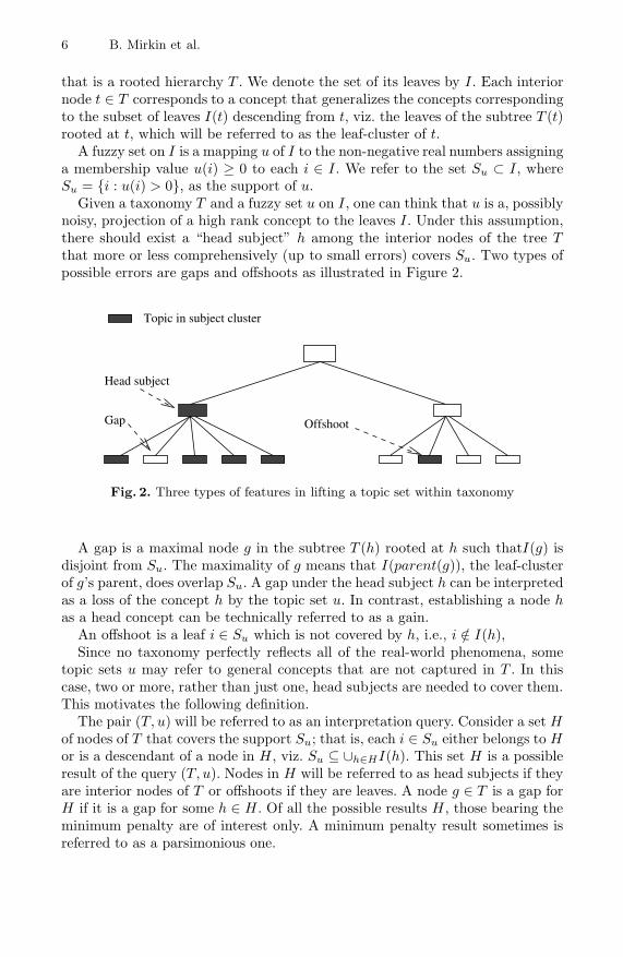
Given a taxonomy T and a fuzzy set u on I, one can think that u is a, possiblynoisy, projection of a high rank concept to the leaves I. Under this assumption,there should exist a “head subject” h among the interior nodes of the tree Tthat more or less comprehensively (up to small errors) covers Su. Two types ofpossible errors are gaps and offshoots as illustrated in Figure 2.
Topic in subject cluster
Gap
Head subject
Offshoot
Fig. 2. Three types of features in lifting a topic set within taxonomy
A gap is a maximal node g in the subtree T (h) rooted at h such thatI(g) isdisjoint from Su. The maximality of g means that I(parent(g)), the leaf-clusterof g’s parent, does overlap Su. A gap under the head subject h can be interpretedas a loss of the concept h by the topic set u. In contrast, establishing a node has a head concept can be technically referred to as a gain.
An offshoot is a leaf i ∈ Su which is not covered by h, i.e., i /∈ I(h),Since no taxonomy perfectly reflects all of the real-world phenomena, some
topic sets u may refer to general concepts that are not captured in T . In thiscase, two or more, rather than just one, head subjects are needed to cover them.This motivates the following definition.
The pair (T, u) will be referred to as an interpretation query. Consider a set Hof nodes of T that covers the support Su; that is, each i ∈ Su either belongs to Hor is a descendant of a node in H , viz. Su ⊆ ∪h∈HI(h). This set H is a possibleresult of the query (T, u). Nodes in H will be referred to as head subjects if theyare interior nodes of T or offshoots if they are leaves. A node g ∈ T is a gap forH if it is a gap for some h ∈ H . Of all the possible results H , those bearing theminimum penalty are of interest only. A minimum penalty result sometimes isreferred to as a parsimonious one.
How to Visualize a Crisp or Fuzzy Topic Set over a Taxonomy 7
Any penalty value p(H) associated with a set of head subjects H shouldpenalize the head subjects, offshoots and gaps commensurate with the weightingof nodes in H determined from the membership values in the topic set u. Weassign the head penalty to be head, offshoot penalty, off, and the gap penalty,gap.
To take into account the u membership values, we need to aggregate them tonodes of higher rank in T . In order to define appropriate membership values forinterior nodes of tree T , we assume one of the following normalization conditions:
(P) Probabilistic condition∑
i∈I
u(i) = 1
(Q) Quadratic condition∑
i∈I
u2(i) = 1
(N) No condition0 ≤ u(i) ≤ 1
We observe that a crisp set S ⊆ I can be considered as a fuzzy set with thenon-zero membership values defined according to the normalization principle.
The three normalization conditions correspond to three possible ways of ag-gregating a set of individual membership values. For each interior node t ∈ T ,its membership weight is defined as follows:
(P) u(t) =∑
i∈I(t) u(i)
(Q) u(t) =√∑
i∈I(t) u(i)2 (1)
(N) u(t) = maxi∈I(t) u(i)
Under each of the definitions, the weight of a gap is zero. The membershipweight of the root is 1 with each of the three normalizations. In the case of acrisp set S with no condition (N), the weight of node t ∈ T is equal to zero ifI(t) is disjoint from S, and it is unity, otherwise.
We now define the notion of pruned tree. Pruning the tree T at t results in thetree remaining after deleting all descendants of t. The definitions in (1) are con-sistent in that the weights of the remaining nodes are unchanged by any sequenceof successive prunings. Note, however, that the sum of the weights assigned tothe leaves in a pruned tree with normalizations (Q) and (N) is typically lessthan that in the original tree. With the normalization (P), it unchanges. Onecan notice, as well, that the decrease of the summary weight at the repeatedpruning of the tree is steeper with no normalization (N).
We consider that weight u(t) of node t influences not only its own contri-bution, but also contributions of those gaps that are children of t. Therefore,the contribution to the penalty value of each of the gaps g of a head subjecth ∈ T is weighted according to the membership weight of its parent, as defined

8 B. Mirkin et al.
by γ(g) = u(parent(g)). Let us denote by Γ (h) the set of all gaps below h. Thegap contribution of h is defined as γ(h) =
∑g∈Γ (h) γ(g). For a crisp query set S
with no condition, (N), this is just the number of gaps in Γ (h).To distinguish between proper head subjects and offshoots in H we denote
the set of leaves and interior nodes in H as H− and H+, respectively.Then our penalty function p(H) for the tree T is defined by:
p(H) = head ×∑
h∈H+
u(h) + gap ×∑
h∈H+
γ(h) + off ×∑
h∈H−u(h).
The problem is to find such a set H that minimizes the penalty - this will bethe result of the query (T, u).
2.2 Lifting Method
A preliminary step is to prune the tree T of irrelevant nodes. We then annotateall interior nodes t ∈ T by extending the leaf membership values as in (1). Thosenodes in the pruned tree that have a zero weight are gaps; they are assignedwith a γ-value which is the u-weight of its parent. This can be accomplished asfollows:
(a) Label with 0 all nodes t whose clusters I(t) do not overlap Su. Then removefrom T all nodes that are children of 0-labeled nodes since they cannot begaps. We note that all the elements of Su are in the leaf set of the prunedtree, and all the other leaves of the pruned tree are labelled 0.
(b) The membership vector u is extended to all nodes of the pruned tree accord-ing to the rules in (1).
(c) Recall that Γ (t) is the set of gaps, that is, the 0-labeled nodes of the prunedtree, and γ(t) =
∑g∈Γ (t) u(parent(g)). We compute γ(t) by recursively as-
signing Γ (t) as the union of the Γ -sets of its children and γ(t) as the sum ofthe γ-values of its children. For leaf nodes, Γ (t) = and γ(t) = 0 if t ∈ Su.Otherwise, i.e. if t is a gap node (or, equivalently, if t is labelled 0), Γ (t) = tand γ(t) = u(parent(t)).
The algorithm proceeds recursively from the leaves to the root. For each node t,we compute two sets, H(t) and L(t), containing those nodes at which gains andlosses of head subjects occur. The respective penalty is computed as p(t).
I InitialisationAt each leaf i ∈ I: If u(i) > 0, define H(i) = i, L(i) = and p(i) =off × u(i).If u(i) = 0, define H(i) = , L(i) = and p(i) = 0.
II RecursionConsider a node t ∈ T having a set of children W , with each child w ∈ Wassigned a pair H(w), L(w) and associated penalty p(w). One of the followingtwo cases must be chosen:

How to Visualize a Crisp or Fuzzy Topic Set over a Taxonomy 9
(a) The head subject has been gained at t, so the sets H(w) and L(w) at itschildren w ∈ W are not relevant. Then H(t), L(t) and p(t) are definedby: H(t) = t;L(t) = Γ (t);p(t) = head × u(t) + gap× γ(t)
(b) The head subject has not been gained at t, so at t we combine the H-and L-sets as follows:
H(t) =⋃
w∈W
H(w), L(t) =⋃
w∈W
L(w) and p(t) =∑
w∈W
p(w).
Choose whichever of (a) and (b) has the smaller value of p(t).III Output: Accept the values at the root:
H(root) - the heads and offshoots, L(root) - the gaps, p(root) - the penalty.
It is not difficult to prove that the algorithm does produce a parsimoniousresult.
3 An Example of Application
Table 1 presents a fuzzy cluster obtained in our project (on the data from asurvey conducted in CENTRIA of Faculdade de Ciencias e Tecnologia, Univer-sidade Nova de Lisboa (DI-FCT-UNL) in 2009) by applying our Fuzzy AdditiveSpectral clustering (FADDIS) algoritm [13]. This cluster is visualized with thelifting method applied at penalty parameter values displayed in Figure 3. Thedescription of the visualization is presented in Table 2.
Table 1. A cluster of research activities undertaken in a research centre
Membership Code ACM-CCSvalue Topic
0.69911 I.5.3 Clustering0.3512 I.5.4 Applications in I.5 PATTERN RECOGNITION0.27438 J.2 PHYSICAL SCIENCES AND ENGINEERING (Applications in)0.1992 I.4.9 Applications in I.4 IMAGE PROCESSING AND COMPUTER VISION0.1992 I.4.6 Segmentation0.19721 H.5.1 Multimedia Information Systems0.17478 H.5.2 User Interfaces0.17478 H.5.3 Group and Organization Interfaces0.16689 H.1.1 Systems and Information0.16689 I.5.1 Models in I.5 PATTERN RECOGNITION0.14453 I.5.2 Design Methodology (Classifiers)0.13646 H.5.0 General in H.5 INFORMATION INTERFACES AND PRESENTATION0.13646 H.0 GENERAL in H. Information Systems0.16513 H.1.2 User/Machine Systems

10 B. Mirkin et al.
Mapping of CENTRIA Cluster 1 on ACM−CCS taxonomy
acmccs98
H.
H.0
H.1
H.1.0 H.1.1 H.1.2 H.1.m
H.2 H.3 H.4
H.5
H.5.0 H.5.1 H.5.2 H.5.3 H.5.4 H.5.5 H.5.m
H.m
I.
I.4
I.4.6 I.4.9 ...
I.5
I.5.0 I.5.1 I.5.2 I.5.3 I.5.4 I.5.5 I.5.m
...
J.
J.2 ...
...
Head SubjectOffshootGap"..." − Not covered
Penalty: Head Subject: 1Offshoot: 0.8Gap: 0.055
Fig. 3. Visualization of the optimal lift of the cluster in Table 1 in the ACM-CCS tree;most irrelevant leaves are not shown for the sake of simplicity
Table 2. Interpretation of the cluster with optimal lifting
HEAD SUBJECTS
H. Information SystemsI.5 PATTERN RECOGNITION
OFFSHOTS
I.4.6 SegmentationI.4.9 ApplicationsJ.2 PHYSICAL SCIENCES AND ENGINEERING
GAPS
H.2 DATABASE MANAGEMENTH.3 INFORMATION STORAGE AND RETRIEVALH.4 INFORMATION SYSTEMS APPLICATIONSH.5.4 Hypertext/HypermediaH.5.5 Sound and Music ComputingI.5.5 Implementation
How to Visualize a Crisp or Fuzzy Topic Set over a Taxonomy 11
4 Conclusion
The lifting method should be a useful addition to the methods for interpretingtopic sets produced by various data analysis tools. Unlike the methods based onthe analysis of frequencies within individual taxonomy nodes, the interpretationcapabilities of this method come from an interplay between the topology of thetaxonomy tree, the membership values and the penalty weights for the headsubjects and associated gap and offshoot events.
On the other hand, the definition of the penalty weights remains of an issue inthe method. One can think that potentially this issue can be overcome by usingthe maximum likelihood approach. This can happen if a taxonomy is used forvisualization queries frequently – then probabilities of the gain and loss eventscan be assigned to each node of the tree. Using this annotation, under usualindependence assumptions, the maximum likelihood criterion would inherit theadditive structure of the minimum penalty criterion. Then the recursions of thelifting algorithm will remain valid, with respective changes in the criterion ofcourse.
We can envisage, that such a development may put the issue of building thetaxonomy tree onto a firm computational footing according to the structureof the flow of queries. An ideal taxonomy in an ideal world would be annotatedwith very contrast, one or zero probabilities, because most query topic sets wouldcoincide with the leaf-clusters. On the contrary, the taxonomy at which the lossprobabilities are similar to each other across the tree may be safely claimedunsuitable for the current query flow.
Acknowledgments
This work has been supported by the grant PTDC/EIA/69988/2006 from thePortuguese Foundation for Science & Technology. B.M. The partial financialsupport of the Laboratory of Choice and Analysis of Decisions at the StateUniversity – Higher School of Economics, Moscow RF, to BM is acknowledged.
References
1. ACM Computing Classification System (1998),http://www.acm.org/about/class/1998 (Cited September 9, 2008)
2. Advanced Visual Systems (AVS),http://www.avs.com/solutions/avs-powerviz/utility_distribution.html
(Cited November 27 2010)3. Beneventano, D., Dahlem, N., El Haoum, S., Hahn, A., Montanari, D., Reinelt,
M.: Ontology-driven semantic mapping. In: Enterprise Interoperability III, PartIV, pp. 329–341. Springer, Heidelberg (2008)
4. Buche, P., Dibie-Barthelemy, J., Ibanescu, L.: Ontology mapping using fuzzy con-ceptual graphs and rules. In: ICCS Supplement, pp. 17–24 (2008)
5. Cali, A., Gottlob, G., Pieris, A.: Advanced processing for ontological queries. Pro-ceedings of the VLDB Endowment 3(1), 554–565 (2010)

12 B. Mirkin et al.
6. Dotan-Cohen, D., Kasif, S., Melkman, A.: Seeing the forest for the trees: using thegene ontology to restructure hierarchical clustering. Bioinformatics 25(14), 1789–1795 (2009)
7. Gahegan, M., Agrawal, R., Jaiswal, A., Luo, J., Soon, K.-H.: A platform for visu-alizing and experimenting with measures of semantic similarity in ontologies andconcept maps. Transactions in GIS 12(6), 713–732 (2008)
8. Ghazvinian, A., Noy, N., Musen, M.: Creating mappings for ontologies inBiomedicine: simple methods work. In: AMIA 2009 Symposium Proceedings, pp.198–202 (2009)
9. Mansingh, G., Osei-Bryson, K.-M., Reichgelt, H.: Using ontologies to facili-tate post-processing of association rules by domain experts. Information Sci-ences 181(3), 419–434 (2011)
10. Marinica, C., Guillet, F.: Improving post-mining of association rules with ontolo-gies. In: The XIII International Conference Applied Stochastic Models and DataAnalysis (ASMDA), pp. 76–80 (2009), ISBN 978-9955-28-463-5
11. Mazza, R.: Introduction to Information Visualization. Springer, London (2009),ISBN: 978-1-84800-218-0
12. Mirkin, B., Nascimento, S., Pereira, L.M.: Cluster-lift method for mapping re-search activities over a concept tree. In: Koronacki, J., Ras, Z.W., Wierzchon, S.T.,Kacprzyk, J. (eds.) Advances in Machine Learning II. SCI, vol. 263, pp. 245–257.Springer, Heidelberg (2010)
13. Mirkin, B., Nascimento, S.: Analysis of Community Structure, Affinity Data andResearch Activities using Additive Fuzzy Spectral Clustering, TR-BBKCS-09-07,p. 24 (2009)
14. OWL 2 Web Ontology Language Overview (2009),http://www.w3.org/TR/2009/RECowl2overview20091027/
(Cited November 27, 2010)15. SNOMED CT (2011),
http://www.connectingforhealth.nhs.uk/systemsandservices/data/uktc/
snomed
(Cited March 2011)16. Sosnovsky, S., Mitrovic, A., Lee, D., Prusilovsky, P., Yudelson, M., Brusilovsky, V.,
Sharma, D.: Towards integration of adaptive educational systems: mapping domainmodels to ontologies. In: Dicheva, D., Harrer, A., Mizoguchi, R. (eds.) Procs. of 6thInternational Workshop on Ontologies and Semantic Web for ELearning (SWEL2008) at ITS 2008 (2008),http://compsci.wssu.edu/iis/swel/SWEL08/Papers/Sosnovsky.pdf
17. Thomas, H., O’Sullivan, D., Brennan, R.: Evaluation of ontology mapping repre-sentation. In: Proceedings of the Workshop on Matching and Meaning, pp. 64–68(2009)

On Merging the Fields of Neural Networks and
Adaptive Data Structures to Yield New PatternRecognition Methodologies
B. John Oommen
School of Computer Science, Carleton University, Ottawa, Canada
Abstract. The aim of this talk is to explain a pioneering exploratory re-search endeavour that attempts to merge two completely different fieldsin Computer Science so as to yield very fascinating results. These arethe well-established fields of Neural Networks (NNs) and Adaptive DataStructures (ADS) respectively. The field of NNs deals with the trainingand learning capabilities of a large number of neurons, each possessingminimal computational properties. On the other hand, the field of ADSconcerns designing, implementing and analyzing data structures whichadaptively change with time so as to optimize some access criteria. In thistalk, we shall demonstrate how these fields can be merged, so that theneural elements are themselves linked together using a data structure.This structure can be a singly-linked or doubly-linked list, or even a Bi-nary Search Tree (BST). While the results themselves are quite generic,in particular, we shall, as a prima facie case, present the results in whicha Self-Organizing Map (SOM) with an underlying BST structure can beadaptively re-structured using conditional rotations. These rotations onthe nodes of the tree are local and are performed in constant time, guar-anteeing a decrease in the Weighted Path Length of the entire tree. Asa result, the algorithm, referred to as the Tree-based Topology-OrientedSOM with Conditional Rotations (TTO-CONROT), converges in such amanner that the neurons are ultimately placed in the input space so asto represent its stochastic distribution. Besides, the neighborhood prop-erties of the neurons suit the best BST that represents the data.
Summary of the Research Contributions
Consider a set A = A1, A2, . . . , AN of records, where each record Ai is identi-fied by a unique key, ki. The records are accessed with respective probabilitiesS = [s1, s2, . . . , sN ], which are assumed unknown. In the field of Adaptive DataStructures (ADS), we try to maintain A in a data structure which is constantlychanging so as to optimize the average or amortized access times. Chancellor’s Professor ; Fellow : IEEE and Fellow : IAPR. The Author also holds
an Adjunct Professorship with the Dept. of ICT, University of Agder, Norway. Theauthor is grateful for the partial support provided by NSERC, the Natural Sciencesand Engineering Research Council of Canada. Although the research associated withthis paper was done together with my students including Rob Cheetham, David Ngand Cesar Astudillo, the future research proposed is truly of an exploratory nature,and in one sense, could be “wishful thinking”.
S.O. Kuznetsov et al. (Eds.): PReMI 2011, LNCS 6744, pp. 13–16, 2011.c© Springer-Verlag Berlin Heidelberg 2011
14 B.J. Oommen
If the data is maintained in a list, adaptation is obtained by invoking a Self-Organizing List (SLL), which is a linear list that rearranges itself each time anelement is accessed. The goal is that the elements are eventually reorganized interms of the descending order of the access probabilities. Many memoryless up-date rules have been developed to achieve this reorganization, [5,8,13,15,16,17].Foremost among these are the well-studied Move-To-Front (MTF), Transposi-tion, the POS(k) and the Move-k-Ahead rules. Schemes involving the use of extramemory have also been developed [16,17]. The most obvious of these, uses coun-ters to achieve the estimation of the access probabilities. Another is a stochasticMove-to-Rear rule due to Oommen and Hansen [15], which moves the accessedelement to the rear with a probability which decreases each time the element isaccessed. Stochastic MTF [15] and various stochastic and deterministic Move-to-Rear schemes [16,17] due to Oommen et. al have also been reported. All ofthese rules can also be used for Doubly-Linked Lists (DLLs), where accesses canbe made from either end of the list.
A Binary Search Tree (BST) may also be used to store the records wherethe keys are members of an ordered set, A. Each record Ai is identified by aunique key, and the records are stored in such a way that a symmetric-ordertraversal of the tree (with respect to the identifying key) will yield the records inan ascending order. The problem of constructing an optimal BST given A and Srequires O(N2) time and space [11]. Generally speaking, all the BST heuristicsuse the primitive Rotation operation [1] to restructure the tree. MemorylessBST schemes also employ the Move-To-Root [4] and Simple Exchange [4] ruleswhich are analogous to the MTF and transposition rules for SLLs. Sleator andTarjan [18] introduced a scheme, which moves the accessed record up to theroot of the tree using the splaying operation – a multi-level generalization ofrotation. Schemes requiring extra memory such as the Monotonic Tree schemeand Melhorn’s D-Tree etc. have also been proposed [14]. In spite of the fact thatSLLs and BSTs could have conflicting reorganization criteria, there is a closemapping between certain SLL heuristics and the corresponding BST heuristicsas reported by Lai and Wood [13]. With regard to Adaptive BSTs, the mosteffective solution is due to Cheetham et al. which uses the concept of ConditionalRotations [6]. The latter paper proposed a solution where an accessed elementis rotated towards the root if and only if the overall Weighted Path Length ofthe resulting BST decreases.
The field of NNs [7,9] deals with the training and learning capabilities of alarge number of computing elements (i.e., the neurons), each possessing minimalcomputational properties. There are scores of families of NNs described in the lit-erature, including the Backpropagation, the Hopfield network, the Neocognitron,the SOM etc. [12]. However, unlike the traditional concepts useful in developingfamilies of NNs, we propose to “link” the neurons together using a data structurewhich can be a SLL, a DLL or even a BST. As far as we know, such an attemptto merge the fields of NNs and ADS is both novel and pioneering.
The advantage of using an ADS is that during the training phase, we canmodify the configuration of the data structure by moving a neuron closer to
Merging Neural Networks and Adaptive Data Structures 15
its head (root), and thus explicitly recording the relevant role of the particularnode with respect to its nearby neurons. This leads us to the concept of NeuralPromotion, which is the process by which a neuron is relocated in a moreprivileged position1 in the network with respect to the other neurons in theneural network. Thus, while “all neurons are born equal”, their importance inthe society of neurons is determined by what they represent. This is achieved,by an explicit advancement of its rank or position.
While the results themselves are quite generic and can potentially lead tomany new avenues for further research, in particular, we shall, as a prima faciecase, present the results [2,3] in which the NN is the Self-Organizing Map (SOM)[12]. Even though numerous researchers have focused on deriving variants of theoriginal SOM strategy, few of the reported results possess the ability of modifyingthe underlying topology, leading to a dynamic modification of the structureof the network by adding and/or deleting nodes and their inter-connections.Moreover, only a small set of strategies use a tree as their underlying datastructure. From our perspective, we believe that it is also possible to gain abetter understanding of the unknown data distribution by performing structuraltree-based modifications on the tree, by rotating the nodes within the BST thatholds the whole structure of neurons. Thus, we attempt to use rotations, tree-based neighbors and the feature space as an effort to enhance the capabilitiesof the SOM by representing the underlying data distribution and its structuremore accurately. Furthermore, as a long term ambition, this might be useful forthe design of faster methods for locating the SOM’s Best Matching Unit.
The prima facie strategy for which we have obtained encouraging resultsis the Tree-based Topology-Oriented SOM with Conditional Rotations (TTO-CONROT). TTO-CONROT has a set of neurons, which, like all SOM-basedmethods, represents the data space in a condensed manner. Secondly, it possessesa connection between the neurons, where the neighbors are based on a learnedtree-based nearness measure. Similar to the reported families of SOMs, a subsetof neurons closest to the BMU are moved towards the sample point using a vectorquantization rule. But, unlike many of the reported SOM families, the identity ofthe neurons moved is based on the tree-based proximity (and not on the feature-space proximity). CONROT-BST achieves neural promotion by performing alocal movement of the node, where only its direct parent and children are awareof the neuron promotion. Finally, the TTO-CONROT incorporates tree-basedmutations, namely the above-mentioned conditional rotations.
Our proposed strategy is adaptive, with regard to the migration of the pointsand with regard to the identity of the neurons moved. Additionally, the distri-bution of the neurons in the feature space mimics the distribution of the samplepoints. Lastly, by virtue of the conditional rotations, it turns out that the entiretree of neurons is optimized with regard to the overall accesses, which is a uniquephenomenon – when compared to the reported family of SOMs.
The potential to extend these results for other NN families and ADSs is open.
1 As far as we know, we are not aware of any research which deals with the issue ofNeural Promotion. Thus, we believe that this concept, itself, is pioneering.

16 B.J. Oommen
References
1. Adel’son-Velski’i, G.M., Landis, E.M.: An algorithm for the organization of infor-mation. Sov. Math. Dokl. 3, 1259–1262 (1962)
2. Astudillo, C.A., Oommen, J.B.: A novel self organizing map which utilizes imposedtree-based topologies. In: Kurzynski, M., Wozniak, M. (eds.) Computer Recogni-tion Systems 3. Computer Recognition, vol. 57, pp. 169–178. Springer, Heidelberg(2009)
3. Astudillo, C.A., Oommen, B.J.: On using adaptive binary search trees to enhanceself organizing maps. In: Nicholson, A., Li, X. (eds.) AI 2009. LNCS, vol. 5866, pp.199–209. Springer, Heidelberg (2009)
4. Allen, B., Munro, I.: Self-organizing binary search trees. Journal of the ACM 25,526–535 (1978)
5. Arnow, D.M., Tenenbaum, A.M.: An investigation of the move-ahead-k rules. In:Proceedings of Congressus Numerantium, Proceedings of the Thirteenth South-eastern Conference on Combinatorics, Graph Theory and Computing, Florida, pp.47–65 (1982)
6. Cheetham, R.P., Oommen, B.J., Ng, D.T.H.: Adaptive structuring of binary searchtrees using conditional rotations. IEEE Transactions on Knowledge and Data En-gineering 5, 695–704 (1993)
7. Duda, R., Hart, P.E., Stork, D.G.: Pattern Classification, 2nd edn. Wiley Inter-science, Hoboken (2000)
8. Gonnet, G.H., Munro, J.I., Suwanda, H.: Exegesis of self-organizing linear search.SIAM Journal of Comput. 10, 613–637 (1981)
9. Haykin, S.: Neural Networks and Learning Machines, 3rd edn. Prentice-Hall, En-glewood Cliffs (2008)
10. Hester, H.J., Herberger, D.S.: Self-organizing linear search. In: ACM ComputingSurveys, pp. 295–311 (1976)
11. Knuth, D.E.: The Art of Computer Programming, vol. 3. Addison-Wesley, Reading(1973)
12. Kohonen, T.: Self-Organizing Maps. Springer-Verlag New York, Inc., Secaucus, NJ,USA (1995)
13. Lai, T.W., Wood, D.: A relationship between self organizing lists and binary searchtrees. In: Proceedings of the 1991 Int. Conf. Computing and Information, May 1991,pp. 111–116 (1991)
14. Mehlhorn, K.: Data Structures and Algorithms 1: Sorting and Searching. Springer,Berlin (1984)
15. Oommen, B.J., Hansen, E.R.: List organizing strategies using stochastic move-to-front and stochastic move-to-rear operations. SIAM Journal of Computing 16,705–716 (1987)
16. Oommen, B.J., Hansen, E.R., Munro, J.I.: Deterministic optimal and expedientmove-to-rear list organizing strategies. Theoretical Computer Science 74, 183–197(1990)
17. Oommen, B.J., Ng, D.T.H.: An optimal absorbing list organization strategy withconstant memory requirements. Theoretical Computer Science 119, 355–361 (1993)
18. Sleator, D.D., Tarjan, R.E.: Self-adjusting binary search trees. Journal of theACM 32, 652–686 (1985)
19. Walker, W.A., Gotlieb, C.C.: A top-down algorithm for constructing nearly optimallexicographical trees. In: Graph Theory and Computing (1972)

Quality of Algorithms for Sequence Comparison
Mikhail Roytberg1,2
1 Institute of Mathematical Problems in Biology RAS, Institutskaya, 4, Pushchino,Moscow Region, 142290, Russia
2 National Research University Higher School of Economics, Myasnitskaya, 20,Moscow, 101000, [email protected]
Abstract. Pair-wise sequence alignment is the basic method of compar-ative analysis of proteins and nucleic acids. Studying the results of thealignment one has to consider two questions: (1) did the program find allthe interesting similarities (“sensitivity”) and (2) are all the found sim-ilarities interesting (“selectivity”). Definitely, one has to specify, whatalignments are considered as the interesting ones. Analogous questionscan be addressed to each of the obtained alignments: (3) which part ofthe aligned positions are aligned correctly (“confidence”) and (4) doesalignment contain all pairs of the corresponding positions of comparedsequences (“accuracy”). Naturally, the answer on the questions dependson the definition of the correct alignment. The presentation addresses theabove two pairs of questions that are extremely important in interpretingof the results of sequence comparison.
Keywords: alignment, seed, sequence comparison, sensitivity, selectiv-ity, accuracy, confidence.
1 Seeds, Sensitivity and Selectivity
Many programs of sequence similarity search (e.g. BLAST, FASTA) are basedon the filtration paradigm; they firstly mark the regions of putative similarityand then restrict the search with the regions only. To perform the first step theseeding scheme is usually implemented: one searches only for the similaritiescontaining the strong similarity of special form, e.g. the similarities containingk consecutive matches. This seeding scheme leads to the drastic speed up com-pared to the more rigorous dynamic programming based methods at the priceof possible loss of some interesting similarities.
In the framework of similarity search in biological sequences, a seed specifiesa class of short sequence motifs which, if shared by two sequences, are assumedto witness a potential similarity. We say that a seed matches a similarity (ora similarity is recognized by a seed) if it contains a sub-similarity correspond-ing to a seed. To define what is sensitivity and selectivity of a seed we have tomake some preliminary definitions. First, we have to describe the set of con-sidered possible sequence alignments and the subset of interesting similarities(“target similarities”). For example, we may consider all ungapped similarities
S.O. Kuznetsov et al. (Eds.): PReMI 2011, LNCS 6744, pp. 17–20, 2011.c© Springer-Verlag Berlin Heidelberg 2011

18 M. Roytberg
(alignments) of a given length and the set of target similarities consisting of allungapped alignments having identity level higher than a given cut-off. Second, wehave to consider the two probability distributions on alignments: the backgrounddistribution, corresponding to the random alignments and the foreground dis-tribution that corresponds to the target alignments. E.g. one can consider bothdistributions as Bernoulli distributions in two-letter alphabet (match-mismatch)and define the probability of match as 0.25 for the background distribution andas (say) 0.7 for the foreground distribution.
Given the set of target alignments and the distributions, the sensitivity of aseed is the probability that a random similarity is recognized by a seed accordingto a foreground distribution and the selectivity of a seed is the probability that arandom similarity is recognized by a seed according to a background distribution.For the Bernoulli distribution the selectivity is often defined as a probability thata seeding similarity can be found for two random independent sequences of alength equal to the seeds length.
The seed implemented in BLASTN program [1] describes a class of k consec-utive matches (default k = 11). The selectivity of the default seed is 0.25k =0.2511 ∼ 10−6 . The sensitivity of the seed for ungapped nucleotide similaritiesof length 64 with 70% identity is ∼ 0.3. Several years ago Ma, Tromp and Li[2] have proposed to use k nonconsecutive letters as a seed. This change surpris-ingly led to a significant improvement of sensitivity without loss of selectivitythat depends only on the desired number of matches k and on the backgroundmatch probability. E.g. the seed 110100110010101111 (1 stands for the matchpositions and 0 stands for “spaces”) has the sensitivity 0.46 with the same num-ber of matches k = 11. The seminal work of Ma, Tromp and Li (2002) havecaused the investigation of various seed models both for nucleic and amino acidsequences, e.g. vector seeds, subset seeds, multyseeds, etc [3]-[12].
We will consider advantages and disadvantages of the models and will presentthe unifying framework to compute the seed sensitivity.
2 Alignments, Accuracy and Confidence
For many applications it is important to evaluate the quality of algorithmi-cally obtained alignments, i.e. how close the algorithmic alignment is to theevolutionarily true one. Here the evolutionarily true alignment is an alignmentsuperimposing the positions originating from the same position of the commonpredecessor [13].
Moreover, it is important not only to know the quantitative measure of theaverage similarity of alignments but also to understand the typical differencesbetween the algorithmic and the evolutionary true alignments. However, theevolutionarily true alignment of given sequences is usually unknown, and thusan approximation is needed.
There are two possible ways to obtain such an approximation: (1) to use arti-ficial sequences pairs obtained according to a proper evolutionary model [14,15]and (2) to use alignments based on the superposition of the protein 3D-structures(that is possible only for the comparison of amino acid sequences) [13,16].

Quality of Algorithms for Sequence Comparison 19
Accuracy and confidence of global and local alignments were studied in severalpapers [13,14], [16]-[19]. The data show that the main difference between thealgorithmic and true alignments is the number of gaps while the average lengthof a gap is approximately the same. Surprisingly, the 3D-structure based proteinalignments contain significant number of ungapped fragments of negative scorethat can not be restored in algorithmic alignments.
The significant gain both in accuracy and in confidence of protein alignmentscan be achieved using the information on the secondary structure (experimen-tally obtained or predicted) [20,21].
Acknowledgments
The work was supported by grant RFBR 09-04-01053-a.
References
1. Altschul, S.F., Gish, W., Miller, W., et al.: Basic local alignment search tool. J.Mol. Biol. 215, 403–410 (1990)
2. Ma, B., Tromp, J., Li, M.: PatternHunter: Fasterand more sensitive homologysearch. Bioinformatics 18(3), 440–445 (2002)
3. Brejova, B., Brown, D.G., Vinar, T.: Optimal Spaced Seeds for Hidden MarkovModels, with Application to Homologous Coding Regions. In: Baeza-Yates, R.,Chavez, E., Crochemore, M. (eds.) CPM 2003. LNCS, vol. 2676, pp. 42–54.Springer, Heidelberg (2003)
4. Brejova, B., Brown, D.G., Vinar, T.: Vector seeds: An extension to spaced seedsallows substantial improvements in sensitivity and specificity. In: Benson, G., Page,R.D.M. (eds.) WABI 2003. LNCS (LNBI), vol. 2812, pp. 39–54. Springer, Heidel-berg (2003)
5. Brejova, B., Brown, D., Vinar, T.: Optimal spaced seeds for homologous codingregions. Journal of Bioinformatics and Computational Biology 1(4), 595–610 (2004)
6. Brown, D.: Optimizing multiple seeds for protein homology search. IEEE Transac-tions on Computational Biology and Bioinformatics 2(1), 29–38 (2005)
7. Buhler, J., Keich, U., Sun, Y.: Designing seeds for similarity search in genomicDNA. In: Proceedings of the 7th Annual International Conference on Compu-tational Molecular Biology (RECOMB 2003), Berlin, Germany, April 2003, pp.67–75. ACM Press, New York (2003)
8. Kucherov, G., Noe, L., Roytberg, M.: Multiseed lossless filtration. IEEE Transac-tions on Computational Biology and Bioinformatics 2(1), 51–61 (2005)
9. Li, M., Ma, B., Kisman, D., Tromp, J.: Pattern Hunter II: Highly sensitive andfast homology search. Journal of Bioinformatics and Computational Biology (2004),Earlier version in GIW 2003 (International Conference on Genome Informatics)
10. Kucherov, G., Noe, L., Roytberg, M.: A unifying framework for seed sensitivityand its application to subset seeds. Journal of Bioinformatics and ComputationalBiology 4(2), 553–569 (2006)
11. Xu, J., Brown, D.G., Li, M., Ma, B.: Optimizing Multiple Spaced Seeds for Ho-mology Search. In: Sahinalp, S.C., Muthukrishnan, S.M., Dogrusoz, U. (eds.) CPM2004. LNCS, vol. 3109, pp. 47–58. Springer, Heidelberg (2004)

20 M. Roytberg
12. Yang, I., Wang, S., Chen, Y., Huang, P., Ye, L., Huang, X., Chao, K.: Efficientmethods for generating optimal single and multiple spaced seeds. In: Proceedingsof the IEEE 4th Symposium on Bioinformatics and Bioengineering(BIBE 2004),Taichung, Taiwan, May 19-21, 2004, pp. 411–416. IEEE Computer Society Press,Los Alamitos (2004)
13. Sunyaev, Bogopolsky, G.A., Oleynikova, N.V., Vlasov, P.K., Finkelstein, A.V.,Roytberg, M.A.: From Analysis of Protein Structural Alignments Toward a NovelApproach to Align Protein Sequences. PROTEINS: Structure, Function, and Bioin-formatics 54(3), 569–582 (2004)
14. Stoye, J., Evers, D., Meyer, F.: Rose: generating sequence families. Bioinformat-ics 14, 157–163 (1998)
15. Polyanovsky, V., Roytberg, M., Tumanyan, V.: Reconstruction of Genuine Pair-Wise Sequence Alignment. J. Comput. Biol. (April 24, 2008) (Epub ahead of print)
16. Vogt, G., Etzold, T., Argos, P.: An assessment of amino acid exchange matrices inaligning protein sequences: the twilight zone revisited. J. Mol. Biol. 249, 816–831(1995)
17. Domingues, F.S., Lackner, P., Andreeva, A., et al.: Structure-based evaluation ofsequence comparison and fold recognition alignment accuracy. J. Mol. Biol. 297,1003–1013 (2000)
18. Mevissen, H.T., Vingron, M.: Quantifying the local reliability of a sequence align-ment. Prot. Eng. 9, 127–132 (1996)
19. Vingron, M., Argos, P.: Determination of reliable regions in protein sequence align-ments. Prot. Eng. 3, 565–569 (1990)
20. Litvinov, I.I., Lobanov, Yu, M., Mironov, A.A., et al.: Information on the SecondaryStructure Improves the Quality of Protein Sequence Alignment. Mol. Biol. 40, 474–480 (2006)
21. Wallqvist, A., Fukunishi, Y., Murphy, L.R., et al.: Iterative sequence/secondarystructure search for protein homologs: Comparison with amino acid sequence align-ments and application to fold recognition in genome databases. Bioinformatics 16,988–1002 (2000)
Problems of Machine Learning
Alexei Ya. Chervonenkis
Institute of Control Sciences, Moscow, [email protected]
The problem of reconstructing dependencies from empirical data became veryimportant in a very large range of applications. Procedures used to solve thisproblem are known as “Methods of Machine Learning” [1,3]. These proceduresinclude methods of regression reconstruction, inverse problems of mathematicalphysics and statistics, machine learning in pattern recognition (for visual andabstract patterns represented by sets of features) and many others. Many webnetwork control problems also belong to this field. The task is to reconstructthe dependency between input and output data as precisely as possible usingempirical data obtained from experiments or statistical observations.
Input data are composed of descriptions (curves, pictures, graphs, texts, mes-sages) of input objects (we denote an input by x) and may be presented byvectors in Euclidian space or vectors of discrete values. In the latter case theymay be sets of discrete features or even textual descriptions. An output value ymay be given by a real value, vector or a discrete value. In the case of patternrecognition problem, output values may be names of classes (patterns), to whichthe input object belongs.
A training set is given by a sequence of pairs (x1, y1), (x2, y2), . . . , (xl, yl). Oneneeds to find a dependency y = F (x) such that forecast output values y∗ = F (x)for new input objects are most close to actual output values y, correspondingto the inputs x. Several schemes of training sequence generation are possible.From the theoretical point of view, it is most convenient to consider that thepairs are generated independently by some constant (but unknown) probabilitydistribution P (x, y), and the same distribution is used to generate new pairs.However, in practice the assumption of independency fails. Sometimes the dis-tribution changes in time. In this case adaptive schemes of learning should beused, where the reconstructed function also changes in time. In some tasks thereis no assumption about existing of any probability distribution on the set ofpairs. Then the solution is to construct a function that properly approximatesreal dependency over its domain. If dependency between input and output vari-ables is linear (or the best linear approximation is looked for), then well knownLeast Square Method is used to estimate the dependency coefficients. Still, if thetraining set is small (not large enough) in comparison with the number of argu-ments, then LSM does not work or works inefficiently. In this case some kindsof regularization are used. If dependency is sought in the class of polynomials offinite degree, then the problem may be reduced to the previous one by addingdegrees of initial arguments. In the case of many arguments it is necessary to
S.O. Kuznetsov et al. (Eds.): PReMI 2011, LNCS 6744, pp. 21–23, 2011.c© Springer-Verlag Berlin Heidelberg 2011

22 A.Y. Chervonenkis
include degree products of initial arguments. In this case, of course, the num-ber of unknown coefficients grows rapidly and the problem becomes intractable.Besides algebraic polynomials, trigonometric ones can be used, or, in general, ex-pansions over preselected system of basis functions. If the dependency is soughtin the form of piece-wise linear or piece-wise continuous function, then the stan-dard least square method cannot be applied and other tools should be used, suchas artificial neural networks. If the number of basis function necessary for properapproximation is too large, then kernel technique may be applied, which allowsone to estimate the function value at a given point or at a set of given points.The so-called inverse problems of mathematical physics and statistics are also ofthis type.
Machine learning in pattern recognition is a particular case of dependency re-construction. Here the output value is the name of a class. This class of problemscovers a very large range of applications from image recognition to recognition ofcertain type of DNA sites, message classification, or recognition of unauthorizedaccess attempts. In all cases of dependency reconstruction, one chooses a prioria certain class of models and then selects from it a model that in a sense is thebest for describing dependency between input and output.
Three general questions arise in relation to any learning approach:
1. Is there a good model in the class that we have chosen?2. May we hope that if the model behaves well on the training set, will it also
behave well on new data?3. Is there an efficient algorithm for selecting a proper model from a given class
of models?
The smaller is the set of models, the closer is the point delivering minimumto empirical risk to the point delivering minimum to the true risk (within theclass). On the other hand, the chance to find a good model within a small classis less than that for a large class. A solution may be as follows: Consider a setof expanding classes and choose the optimal size of a class, depending on thesize of the training sample. For example, it is possible to increase (or decrease)the degree of approximating polynomial, or increase the number of terms intrigonometric expansion (or expansion over any other system of basic functions).In the case of linear function it is possible to define an order on the argumentsand then sequentially increase the number of input variables in this order. Onealso can look over all combinations of arguments, increasing their number. In thecase of piece-wise linear approximation one may change the number of pieces ornumber of neurons of the artificial neural network.
How one can find the best size of the class? The simplest way is to reservea part of data set given for learning (validation set), using the rest part forfinding the best model within expanding classes and then testing the resultusing the validation set, and at last selecting the model with the best score onthe validation test. However, usually training data are lacking and it is costly toreserve some part of it. In this case one can use a means of control that does notneed reservation, e.g. cross-validation. Another way is to estimate analytically
Problems of Machine Learning 23
the difference between empirical and real risk values depending on training dataand the size of a class from which we select the best model. The reason is thatthe empirical risk always deceases (not increases) with the class size, while thetrue risk passing its minimum starts increasing with the class size. Analytically itis possible to determine a corresponding correction. Other methods for choosingoptimal complexity of a decision are possible. Note that the model complexitydoes not always directly correlates with the size of a class of models. For example,some very complicated procedures of feature preprocessing may be proposed, andthe best decision rule is sought for a narrow class described in terms of secondaryfeatures resulting from preprocessing.
Let us consider in more detail some principles of choosing optimal model com-plexity within analytical approach. It is well known that maximum likelihoodprinciple gives good results if the number of model parameters is rather lowin comparison with the size of training data. On the other hand, Bayesian ap-proach [2] gives the optimal result in the case where the number of parametersis very large or even infinite, but it requires a priori distribution over the setof their possible values. This approach results in a form of regularization, andit gives optimal degree of the selected model complexity. But how one can findthis a priori distribution? Bayesian approach does not give any answer to thisquestion. However, in many cases the a priori distribution depends on few pa-rameters. Hence, it is promising to hybridize maximum likelihood and Bayesianapproaches [4]: constructing likelihood function for the parameters of the a prioridistribution, finding their optimal value and using them in Bayesian method. Insome cases this approach gives very efficient algorithms.
Another idea is to use analytical estimates of the uniform closeness of em-pirical risk to the true risk (in absolute or relative form) and to use them asthe estimates of the difference between empirical and real risk values. Then itis possible to use the estimates for choosing the best model complexity as it ismentioned above.
References
1. Vapnik, V.N., Chervonenkis, A.Y.: Theory of Pattern Recognition (in Russian).Moscow, Nauka (1974)
2. MacKay, J.D.C.: Bayesian interpolation. Neural Computation 4(3), 415–447 (1992)3. Vapnik, V.N.: The Nature of Statistical Learning Theory. Springer, Heidelberg
(2000)4. Chervonenkis, A.Y.: A combined Bayes - Maximum Likelihood method for regres-
sion. In: Riccia, G.D., Lenz, H.-J., Kruse, R. (eds.) Data Fusion and Perception,Springer, Wien, New-York (2001)

Bayesian Approach to the Pattern Recognition
Problem in Nonstationary Environment
O.V. Krasotkina1, V.V. Mottl2, and P.A. Turkov1
1 Tula State University, Tula, [email protected]
2 Computing Centre of RAS
Abstract. The classical learning problem of the pattern recognition ina finite-dimensional linear space of real-valued features is studied un-der the conditions of a non-stationary universe. The training criterionof non-stationary pattern recognition is formulated as a generalizationof the classical Support Vector Machine. The respective numerical algo-rithm has the computation complexity proportional to the length of thetraining time series.
The majority of modern methods for pattern recognition works under the as-sumption that properties of the environment and consequently required decisionrule doesn’t change in a process of data collection as well as during the exam.However, recently there have appeared many applications, in which samplesof training set are entering the system over a long period of time, when theproperties of the analyzed phenomenon may undergo considerable changes. Theexample of such problem is task of filtering irrelevant or publicity hyperlinks as aresult of retrieval request. The behavior of internet advertising distributors con-stantly turns and it causes changes of publicity hyperlinks features that shouldresult in the adequate correction of search mechanism. Often in this kind of tasksboth the nature of changes in the environment and the fact of changes itself arehidden from direct observation and this makes learning even more difficult. Inliterature this problem is called concept drift [1].
At present there are three approaches to the construction of algorithms takinginto account non-stationary character of decision rule: algorithms based on se-lecting instances, algorithms based on weighted instances and algorithms basedon classifier selection and mergers. The goal of algorithms using selection of in-stances is the choice of prototypes which are relevant for decision rule at thepresent moment. As a rule, it is realized with the help of running window tech-nology when decision rule at the present moment is made only on the basis of theinstances obtained from previous time points. The examples of such algorithmscan be FLORA family of algorithms [1] and TMF [2].
Algorithms based on weighting of instances [3] obtained from different timepoints use the ability of some learning algorithms such as Support Vector Ma-chines (SVMs) method to assign weights to different instances. As a rule, weightsare assigned to the instances according to their ”age” (e.g. period of time fromtheir obtaining).
S.O. Kuznetsov et al. (Eds.): PReMI 2011, LNCS 6744, pp. 24–29, 2011.c© Springer-Verlag Berlin Heidelberg 2011
Bayesian Approach to the Pattern Recognition Problem 25
By ensemble-based approach [5] for pattern recognition in non-stationaryenvironment, required decision rule is made as voting or weighted voting ofclassifiers obtained for different conditions. For example, in the paper [4] it isproposed to cluster training samples and to construct its own classifier for eachcluster.
In general, we can mark that all existing algorithms are more or less heuris-tic and a certain set of heuristics is determined by a specificity of the currenttask. In this paper we propose stochastic concept of the non-stationary environ-ment based on Bayesian approach to the pattern recognition problem. The maininstantaneous property of the non-stationary environment is understood as time-dependent separating hyperplane that in the best way describes the differencesbetween feature vectors of samples of two classes. The proposed concept bringsabout the learning algorithm that is a generalization of the classical SVM forthe case when the parameters of the separating hyperplane change with time.
1 Bayesian Definition of the Pattern RecognitionProblem in Non-stationary Environment
Let every instance of the environment ω ∈ Ω is presented by a point in the linearfeature space x(ω) =
(x1(ω), . . . , xn(ω)
) ∈ Rn, and its hidden membership in
one of two classes is determined by an index value of the class y(ω) ∈ 1,−1.The paper [6] proposed a stochastic model of the universe. The main modelassumption is a priori parametric distribution of the instances
φ (x|a, b, y; c) =
const, yz (a,x) ≥ 1,
e−c(1−yz(a,x)), yz (a,x) < 1,(1)
And this distribution is defined by the objectively existing hyperplane z(x,a) =aT x + b = 0 with an unknown directing vector of features a = (a1, a2, ..., an),having a priori distribution Ψ(a, b|σ2) ∝ exp
(− 12σ2 aT a
). Using the maximum
a posteriori probability principle for the directing vector parameters estimation(a, b) leads us to the widely-known support vector criterion
⎧⎨
⎩J(a, b, δ1, ..., δN |c)= aT a + c
N∑j=1
δj → min,
yj
(aTa + b
)≥1−δj, δj ≥ 0, j = 1, ..., N,
(2)
that was proposed by V. N. Vapnik from a strictly deterministic point of view.Of course, the concept of time is completely absent here.
The principal distinction of the concept of non-stationary environment givenin this paper consists in taking into consideration time factor t. We suppose thatthe main property of non-stationary environment is expressed by time-dependentseparating hyperplane that characterizes primary difference of the feature vectorsof instances of two classes. This separating hyperplane, in turn, is completelydefined by its own direction vector and location parameter, which should beconsidered as time functions at bt: ft
(x(ω)
)= aT
t x + bt. In the terms of the
26 O.V. Krasotkina, V.V. Mottl, and P.A. Turkov
improper probability distributions of two classes in the feature space such idea isformulated in the form of hypothesis that parameters of this pair of distributionsare time varying:
φ (x|at, bt, y; c) =
const, yz(at,x)≥1,e−c(1−yz(at,x)), yz(at,x)<1,
(3)
where z(x, at) = aTt x + b = 0.
We will suppose that at the zero time moment a priori distribution of the sep-arating hyperplane is improper and has the appearance: ψ0(a0, b0) ∝ ψ0(a0) =N(a0|0, I). In turn we will regard directing vector aj as a stochastic stationaryprocess: at = qat−1 + ξ t, M (ξ t) = 0, M(ξ tξ
Tt ) = dI, 0 ≤ q < 1.
2 Dynamic Support Vector Machine Criterion
Now every instance ω ∈ Ω is considered only together with the indication of timepoint when this instance was presented (ω, t). As a result the training set repre-sents as the set of triplet
(Xt ∈ R
n, Yt, t)T
t=1, (Xt,Yt) = (xk,t, yk,t)Nt
k=1 -a subset of instances, entered in time point t.
We obtain the sought-for sequence (at, bt)Tt=1 as maximum point of joint a
priori distribution of separating hyperplane’s parameters and training sample.The maximum a posteriori probability principle lets to the criterion
J(at, bt, δt,j , t = 0, ..., T ) = aT0 a0 + 1
d
T∑t=1
(at − qat−1)T (at − qat−1)+
+ 1d′
T∑t=1
(bt − bt−1)2 +
T∑t=1
Nt∑j=1
δj,t → min[at,bt]Tt=1
yj,t(aTt xj,t + bt) ≥ 1 − δj,t, δj,t ≥ 0, j = 1, . . . , Nt, t = 1, ..., T
(4)
The criterion (4) realizes the conception of the rather smooth sequence of opti-mal separating hyperplanes as opposed to the conception of the single optimalhyperplane in (2).
As the classic learning problem, the dynamical problem (4) is a quadraticprogramming problem but contains T (n + 1) + N variables in contrast to (n +1)+N variables in (2). It is known that a computational complexity of the generalquadratic programming problem is proportional to the cube of the number ofvariables, i.e. a dynamic problem ex facte is more complex than the classicalproblem.
But the objective function in a dynamic problem (4) is pair-wise separable, i.e.representing a sum of private functions every of which depends on the variablesconnected with one or two time points in their increasing order. The algorithmof the pair-wise separable criterion optimization suggested in this paper consistsin an approximate implementation of the dynamic programming procedure andpermits to solve the problem mentioned above within the number of iterationsproportional to the length of the training sequence.

Bayesian Approach to the Pattern Recognition Problem 27
3 Quickly Optimization Procedure for a Dynamic SVMCriterion
The algorithm for the optimization of the obtained pair-wise separable criterionproposed in this paper is based on the using a general principle of the dynamic
programming. Let us to introduce the following notation zt =[z′Tt z′′
t
]T, z′t =
[aT
t bt
]T, z′′t = [δj]
Nt
j=1:
ζt(z′t) = (z′t − z0t )T Q0
t (z′t − z0t ), χt(z′′t) = CeT
t z′′t, et = [1]Nt
1 , t = 1, ..., T,γt(z′t−1, z′t) = (z′t − Ajz′t−1)T Uj(z′t − Ajz′t−1)
and rewrite the criterion (4) in a more convenient form
J(z0, ..., zT ) =T∑
t=0
ζt(z′t) +T∑
t=0
χ(z′′t ) +T∑
t=1
γt(z′t−1, z′t) → min, zt ∈ Zt
where the areas of acceptable values for variables are determined by the condi-tionsz ∈ Rn+2 : gT
j · z′t + z′′j − 1 ≥ 0 , j = (Nt−1 + 1), ..., Nt, t = 0, ..., T, z′′t ≥ 0The central idea of the dynamical programming method uses the concept of asequence of Bellman functions Jt(zt) = min
z0,...,zt−1Jt([zs]ts=1), [zs ∈ Zs]t−1
s=0, con-
nected with partial criteria Jt(z0, ..., zt)=t∑
s=0ζs(z′s)+
t∑s=0
χ(zs)+t∑
s=1γs(z′s−1, zs
′)
having the same structure as the full objective function but defined on the setof variables Zt = (zs, s = 0, ..., t). In order to obtain the filtering estimations ofthe separating hyperplane’s parameters we will use the fundamental property ofBellman function
Jt(zt) = ζt(z′t) + χ(z′′t) + minz′′
t−1,z′′t−1
[γt(z′t−1, z′t) + Jt−1(zt−1)
], (5)
which is called the direct recurrence relation. The procedure begins with thefirst Bellman function J0(z0) = ζ0(z0
′) + χ(z′′0). Then Bellman functions arerecurrently evaluated for the following observation. And the minimum of Bellmanfunction on every step determines the filtering value of the parameters of theoptimal separating hyperplane
zt = arg minzt
Jt(zt), zt ∈ Zt. (6)
The optimization procedure is based on the hypothesis that there exists an ap-propriate compact form for Bellman functions representation, allowed to storethis functions in the memory. But in the case then inequality constraints areimposed upon the sought-for variables and the Bellman functions are piecewisequadratic and consequently the dynamic programming procedure cannot be ap-plied immediately. In order to save the computation advantages of the dynamicprogramming procedure we use here the following trick.

28 O.V. Krasotkina, V.V. Mottl, and P.A. Turkov
We heuristically replace the non quadratic functions Ft(z′t) =min
zt−1∈Zt−1
[γt(z′t−1, z′t) + Jt−1(zt−1)
]by the some appropriate quadratic ap-
proximation Ft(z′t) = ct + (z′t − zt)T Qt(z′t − zt). Then the following approx-imations of Bellman functions will be quadratic too and a numerical imple-mentation of the dynamic programming procedure will be possible. Thus, thequadratic approximation of the Bellman function comes to the selection of ap-propriate values of the parameters (ct, zt, Qt) of the quadratic function Ft(z′t),which would ensure invariance conservation of the main features of, generallyspeaking, non-quadratic function and consequently the initial Bellman function.Such features are the minimum point position zt = argminFt(z′t), minimumpoint value ct = min Ft(z′t) , and also the matrix of the second derivatives at theminimum point Qt = ∇2Ft(z′t)
∣∣arg min Ft(z′
t).
4 Case Study: Spam-Filtering Problem
The object of the experimental study in this paper is the problem of filteringspam-addresses in a result of retrieval request. The behavior of distributors ofnetwork advertising constantly improves and as a result a classifier of advertis-ing links used by a search engine should adapt to the behavior of spammers.Consequently we come to problem of construction the time-dependent decisionrule.
As the training data we took an anonymous set of hyperlinks URL ReputationData Set from the repository UCI, first described in the paper [7]. This setconsists of the addresses of Web resources for 121 days grouped according to theobservation days and contains both advertising and relevant hyperlinks. Everyinstance in the data base is characterized by 3.2 million features which may bedivided into two groups: lexical (hostname, primary domain, TLD and etc.) andhost-based (WHOIS info, IP prefix, geographic and etc.). The values of featuresare normalized from 0 to 1, and the features themselves are anonymous. Forcarrying out the experiments from this data base in different ways there havebeen randomly selected 10 instances for each of 11 days taken from the 1st to the110th day with the step of 10 days. The testing set was comprised by accidentallyselected 4000 instances of the 120th day. We deleted the features with the valuesthat are equal on all instances of the training set out of feature descriptions of theinstances participating in the experiment, the number of the rest was 326. Theexperiment was repeated for different sets of training instances. Two algorithmswere compared in the course of the experiment: normal support vector machinewith the hyperplane, constructed on all instances of the training set and thealgorithm of successive refinement of the decision rule, suggested in the paper.In the proposed algorithm of dynamic pattern recognition the parameters ofthe required decision rule d and d′ were chosen by cross-validation procedure,on each iteration of which non-stationary decision rule was constructed withouttaking into account the instances entered over one of the days. The general percent of erroneously classified links ε was calculated for each algorithm: the per
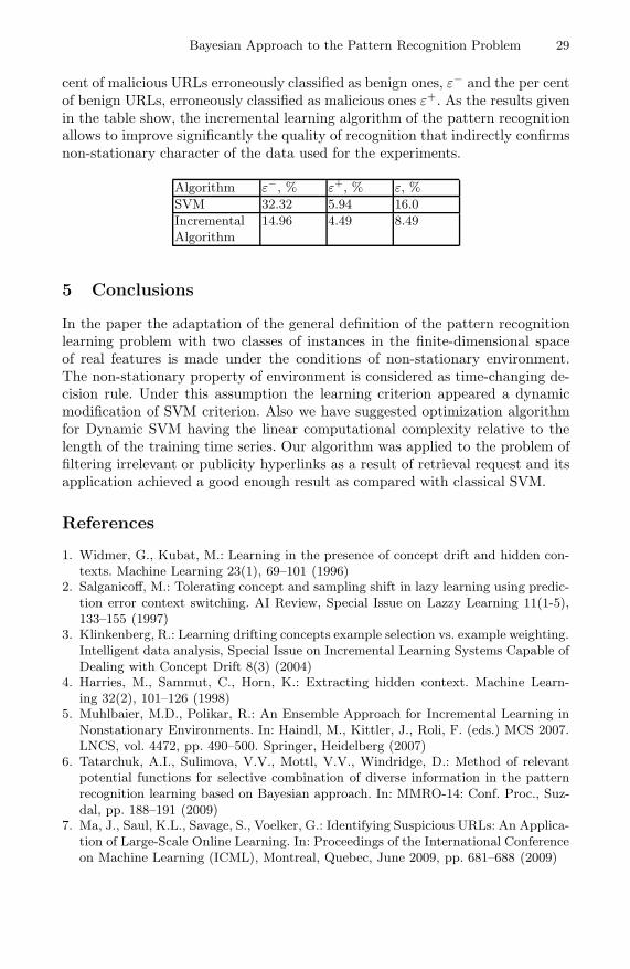
Bayesian Approach to the Pattern Recognition Problem 29
cent of malicious URLs erroneously classified as benign ones, ε− and the per centof benign URLs, erroneously classified as malicious ones ε+. As the results givenin the table show, the incremental learning algorithm of the pattern recognitionallows to improve significantly the quality of recognition that indirectly confirmsnon-stationary character of the data used for the experiments.
Algorithm ε−, % ε+, % ε, %
SVM 32.32 5.94 16.0
IncrementalAlgorithm
14.96 4.49 8.49
5 Conclusions
In the paper the adaptation of the general definition of the pattern recognitionlearning problem with two classes of instances in the finite-dimensional spaceof real features is made under the conditions of non-stationary environment.The non-stationary property of environment is considered as time-changing de-cision rule. Under this assumption the learning criterion appeared a dynamicmodification of SVM criterion. Also we have suggested optimization algorithmfor Dynamic SVM having the linear computational complexity relative to thelength of the training time series. Our algorithm was applied to the problem offiltering irrelevant or publicity hyperlinks as a result of retrieval request and itsapplication achieved a good enough result as compared with classical SVM.
References
1. Widmer, G., Kubat, M.: Learning in the presence of concept drift and hidden con-texts. Machine Learning 23(1), 69–101 (1996)
2. Salganicoff, M.: Tolerating concept and sampling shift in lazy learning using predic-tion error context switching. AI Review, Special Issue on Lazzy Learning 11(1-5),133–155 (1997)
3. Klinkenberg, R.: Learning drifting concepts example selection vs. example weighting.Intelligent data analysis, Special Issue on Incremental Learning Systems Capable ofDealing with Concept Drift 8(3) (2004)
4. Harries, M., Sammut, C., Horn, K.: Extracting hidden context. Machine Learn-ing 32(2), 101–126 (1998)
5. Muhlbaier, M.D., Polikar, R.: An Ensemble Approach for Incremental Learning inNonstationary Environments. In: Haindl, M., Kittler, J., Roli, F. (eds.) MCS 2007.LNCS, vol. 4472, pp. 490–500. Springer, Heidelberg (2007)
6. Tatarchuk, A.I., Sulimova, V.V., Mottl, V.V., Windridge, D.: Method of relevantpotential functions for selective combination of diverse information in the patternrecognition learning based on Bayesian approach. In: MMRO-14: Conf. Proc., Suz-dal, pp. 188–191 (2009)
7. Ma, J., Saul, K.L., Savage, S., Voelker, G.: Identifying Suspicious URLs: An Applica-tion of Large-Scale Online Learning. In: Proceedings of the International Conferenceon Machine Learning (ICML), Montreal, Quebec, June 2009, pp. 681–688 (2009)
The Classification of Noisy Sequences Generated
by Similar HMMs
A.A. Popov and T.A. Gultyaeva
Department of Software and Database Engineering,Novosibirsk State Technical University, [email protected], gult [email protected]
Abstract. The method for classification performance improvement us-ing hidden Markov models (HMM) is proposed. The k-nearest neighbors(kNN) classifier is used in the feature space produced by these HMM.Only the similar models with the noisy original sequences assumptionare discussed. The research results on simulated data for two-class clas-sification problem are presented.
Keywords: Hidden Markov Model, Derivation, k Nearest Neighbors.
1 Introduction
HMM are a powerful tool for modeling of various processes and pattern recog-nition. By their nature, Markov models allow to deal with spatial-temporal se-quence characteristics directly and therefore they became widely-used [1], [2],[3]. However, despite a wide circulation of models of this kind, HMM possesslow enough classification abilities. Though these models are widespread HMMpossess of sufficiently low classification properties. At the same time it is wellknown that the HMM have a fairly low classification ability.We understand theclassification problem by the following. We have an object set discriminated onclasses by expert (training with teacher). This object set is named the trainingset. We want to create an algorithm that will be able to classify a test objectfrom origin set. The two-class classification problem using the matrix of dis-tances between the objects is discussed in this article. In this case, the eachobject is being described by distances to all other objects from training set. Themethod of the nearest neighbors, the Parzen windows method and the methodof potential functions work with input data of such type. The set of Gaussiantime sequences generated by two HMMs with similar parameters are taken asclassification objects. In order to approximate real-world examples all observedtime sequences being distorted. The task was to compare the capabilities of tra-ditional methods of classification with a simple nearest neighbor classifier [4] inthe space of first derivatives of the likelihood function for the HMM parameters.
The remainder of this article is organized as follows. Section 2 introduces themethod of solution of assigned task. Section 3 provides some results of compu-tational experiments. Section 4 summarizes our findings.
S.O. Kuznetsov et al. (Eds.): PReMI 2011, LNCS 6744, pp. 30–35, 2011.c© Springer-Verlag Berlin Heidelberg 2011

The Classification of Noisy Sequences Generated by Similar HMMs 31
2 The Method of Sequences Classification
An HMM is completely described by the following parameters:
1. The initial state distribution Π = πi, i = 1, N , where πi = Pq1 = i andN – is the number of hidden states in the model.
2. The matrix of state transition probabilities A = aij,where aij = Pqt = j|qt−1 = i, i, j = 1, N , t = 1, T , where T – is the lengthof observable sequence.
3. The matrix of observation symbols probabilities B = bij, i = 1, N ,j = 1, M , where bi(j) = Pot = vj |qt = i, ot – is the symbol observed atthe moment of time t = 1, T , M – is the number of observation states in themodel. In this work the case when function observable symbol probabilitiedistribution is described by a mix of normal distributions is considered insuch a manner that the one hidden state is associated with one observablestate: bi(t) = (
√2πσi)e−(ot−μi)
2/2σ2i ,i = 1, N , t = 1, T .
Thus, HMM is completely described by the matrix of state transition proba-bilities, the probabilities of observation symbols and the initial state distribution:λ = (A, B, π).
A classifier based on log-likelihood function is traditionally used. The sequenceO is considered as being generated by model λ1 if (1) is satisfied:
lnL(O|λ1) > lnL(O|λ2). (1)
Otherwise, it is considered that the sequence is generated by model λ2.Some authors (e.g. [5],[6]) propose to use the spaces of the so-called sec-
ondary features as a feature space in which the sequences are being classified.For example, forward-probabilities and backward-probabilities, which are usedfor computation of probability that the sequence is generated by model λ, can beused as a secondary features. The first derivatives of space of likelihood functionlogarithm are also used. These derivatives are being taken with respect to differ-ent model parameters. The authors [5] offer to include the original sequence intothe feature vector also. In this work the performance of two-class classificationin the space of the first derivatives of the likelihood function is discussed.
The classification problem states as follows. There are two groups of trainingsequences: the first group consists of sequences generated by λ1, and the secondgroup – by λ2. Usually, in order to determine which class the test sequence Otest
is belongs to the rule (1) is used. Because the model parameters λ1 and λ2 areunknown, at first one needs to estimate them (for example, the algorithm ofBaum-Welch is used for it), and then calculate them according to rule (1).
If the competing models have similar parameters, and the observed sequencesare not purely Gaussian sequence, the traditional classification technique using(1) does not always give acceptable results.
The following schema that increases discriminating features of HMM.
Step 1. For each training sequence Olearni
l , i = 1, Kl, l = 1, 2 where Kl – thecount of training sequences for class with number l, the characteristic vector
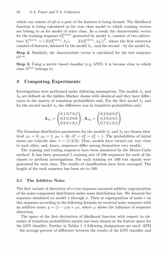
32 A.A. Popov and T.A. Gultyaeva
which can consist of all or a part of the features is being formed. The likelihoodfunction is being calculated as for true class model to which training vectorsare belong to as for model of other class. As a result the characteristic vectorfor the training sequence Olearni
l generated by model λ1 consists of two subvec-tors: V learni
l = (Z(Olearni
l , λ1), Z(Olearni
l , λ2) )T , where the first subvectorconsists of features, initiated by the model λ1 , and the second – by the model λ2.
Step 2. Similarly, the characteristic vector is calculated for the test sequenceOtest.
Step 3. Using a metric based classifier (e.g. kNN) it is become clear to whichclass Otest belongs to.
3 Computing Experiments
Investigations were performed under following assumptions. The models λ1 andλ2 are defined on the hidden Markov chains with identical and they have differ-ences in the matrix of transition probabilities only. For the first model λ1 andfor the second model λ2 the difference was in transitive probabilities only:
Aλ1 =
⎛
⎝0.1 0.7 0.20.2 0.2 0.60.8 0.1 0.1
⎞
⎠ , Aλ2 =
⎛
⎝0.2 0.6 0.20.2 0.3 0.50.7 0.1 0.2
⎞
⎠ .
The Gaussian distribution parameters for the models λ1 and λ2 are chosen iden-tical: μ1 = 0, μ2 = 5, μ3 = 10, σ2
1 = σ22 = σ2
3 = 1. The probabilities of initialstates are coincide also: π = (1, 0, 0). Thus, models have turned out very closeto each other, and, hence, sequences differ among themselves very weakly.
The training and testing sequences have been simulated by the Monte-Carlomethod. It has been generated 5 training sets of 100 sequences for each of theclasses to perform investigations. For each training set 500 test signals weregenerated for each class. The results of classification have been averaged. Thelength of the each sequence has been set to 100.
3.1 The Additive Noise
The first variant of distortion of a true sequence assumed additive superpositionof the noise component distributed under some distribution law. We denoted thesequence simulated on model λ through u. Then at superposition of noise e onthis sequence according to the following formula we received noisy sequence withan additive noise: y = (1 − ω)u + ωe, where ω shows the influence of sequencedistortion.
The space of the first derivatives of likelihood function with respect to ele-ments of transition probabilities matrix has been chosen as the feature space forthe kNN classifier. Further in Tables 1–3 following designations are used: APD– the average percent of difference between the results of the kNN classifier and
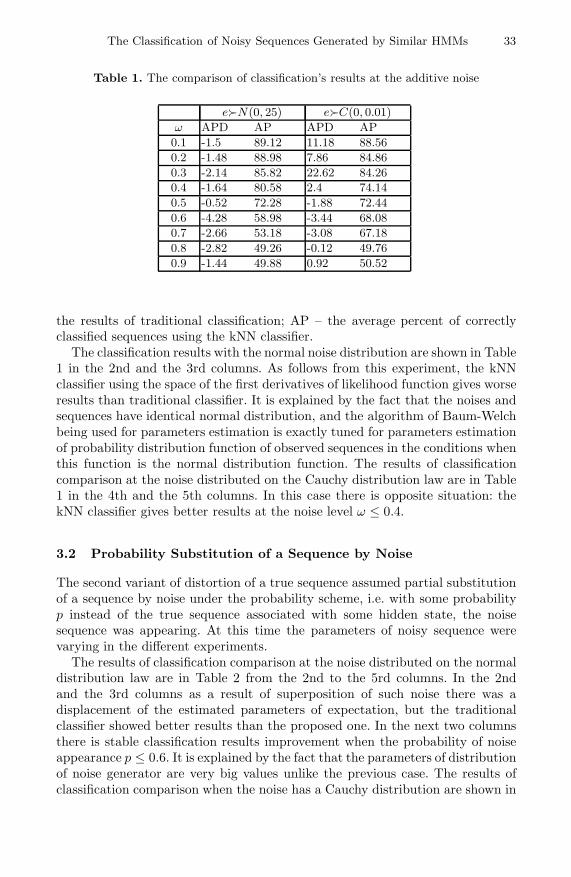
The Classification of Noisy Sequences Generated by Similar HMMs 33
Table 1. The comparison of classification’s results at the additive noise
eN(0, 25) eC(0, 0.01)
ω APD AP APD AP
0.1 -1.5 89.12 11.18 88.56
0.2 -1.48 88.98 7.86 84.86
0.3 -2.14 85.82 22.62 84.260.4 -1.64 80.58 2.4 74.14
0.5 -0.52 72.28 -1.88 72.44
0.6 -4.28 58.98 -3.44 68.08
0.7 -2.66 53.18 -3.08 67.18
0.8 -2.82 49.26 -0.12 49.76
0.9 -1.44 49.88 0.92 50.52
the results of traditional classification; AP – the average percent of correctlyclassified sequences using the kNN classifier.
The classification results with the normal noise distribution are shown in Table1 in the 2nd and the 3rd columns. As follows from this experiment, the kNNclassifier using the space of the first derivatives of likelihood function gives worseresults than traditional classifier. It is explained by the fact that the noises andsequences have identical normal distribution, and the algorithm of Baum-Welchbeing used for parameters estimation is exactly tuned for parameters estimationof probability distribution function of observed sequences in the conditions whenthis function is the normal distribution function. The results of classificationcomparison at the noise distributed on the Cauchy distribution law are in Table1 in the 4th and the 5th columns. In this case there is opposite situation: thekNN classifier gives better results at the noise level ω ≤ 0.4.
3.2 Probability Substitution of a Sequence by Noise
The second variant of distortion of a true sequence assumed partial substitutionof a sequence by noise under the probability scheme, i.e. with some probabilityp instead of the true sequence associated with some hidden state, the noisesequence was appearing. At this time the parameters of noisy sequence werevarying in the different experiments.
The results of classification comparison at the noise distributed on the normaldistribution law are in Table 2 from the 2nd to the 5rd columns. In the 2ndand the 3rd columns as a result of superposition of such noise there was adisplacement of the estimated parameters of expectation, but the traditionalclassifier showed better results than the proposed one. In the next two columnsthere is stable classification results improvement when the probability of noiseappearance p ≤ 0.6. It is explained by the fact that the parameters of distributionof noise generator are very big values unlike the previous case. The results ofclassification comparison when the noise has a Cauchy distribution are shown in
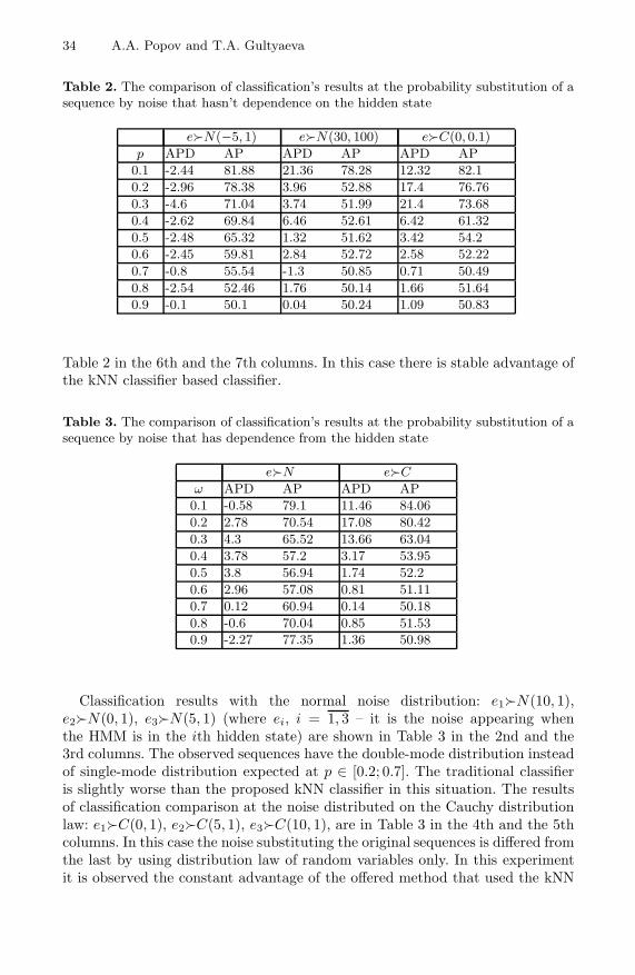
34 A.A. Popov and T.A. Gultyaeva
Table 2. The comparison of classification’s results at the probability substitution of asequence by noise that hasn’t dependence on the hidden state
eN(−5, 1) eN(30, 100) eC(0, 0.1)
p APD AP APD AP APD AP
0.1 -2.44 81.88 21.36 78.28 12.32 82.1
0.2 -2.96 78.38 3.96 52.88 17.4 76.76
0.3 -4.6 71.04 3.74 51.99 21.4 73.68
0.4 -2.62 69.84 6.46 52.61 6.42 61.32
0.5 -2.48 65.32 1.32 51.62 3.42 54.2
0.6 -2.45 59.81 2.84 52.72 2.58 52.22
0.7 -0.8 55.54 -1.3 50.85 0.71 50.49
0.8 -2.54 52.46 1.76 50.14 1.66 51.64
0.9 -0.1 50.1 0.04 50.24 1.09 50.83
Table 2 in the 6th and the 7th columns. In this case there is stable advantage ofthe kNN classifier based classifier.
Table 3. The comparison of classification’s results at the probability substitution of asequence by noise that has dependence from the hidden state
eN eC
ω APD AP APD AP
0.1 -0.58 79.1 11.46 84.06
0.2 2.78 70.54 17.08 80.42
0.3 4.3 65.52 13.66 63.04
0.4 3.78 57.2 3.17 53.95
0.5 3.8 56.94 1.74 52.2
0.6 2.96 57.08 0.81 51.11
0.7 0.12 60.94 0.14 50.18
0.8 -0.6 70.04 0.85 51.530.9 -2.27 77.35 1.36 50.98
Classification results with the normal noise distribution: e1N(10, 1),e2N(0, 1), e3N(5, 1) (where ei, i = 1, 3 – it is the noise appearing whenthe HMM is in the ith hidden state) are shown in Table 3 in the 2nd and the3rd columns. The observed sequences have the double-mode distribution insteadof single-mode distribution expected at p ∈ [0.2; 0.7]. The traditional classifieris slightly worse than the proposed kNN classifier in this situation. The resultsof classification comparison at the noise distributed on the Cauchy distributionlaw: e1C(0, 1), e2C(5, 1), e3C(10, 1), are in Table 3 in the 4th and the 5thcolumns. In this case the noise substituting the original sequences is differed fromthe last by using distribution law of random variables only. In this experimentit is observed the constant advantage of the offered method that used the kNN

The Classification of Noisy Sequences Generated by Similar HMMs 35
classifier. Similar results were obtained in the noise parameters distributed byCauchy distribution law: e1C(0, 1), e2C(0, 0.5), e3C(0, 0.1), i.e. with theabsence of noise displacement but with different scale of distribution.
4 Conclusion
In this article it was shown that the feature space generated by the HMM canbe used for the classification of sequences generated by the similar models. Thefirst derivatives of likelihood function logarithm with respect to the parameters ofHMM were used as the features. The kNN classifier was used in this feature space.Studies have shown that with similar models and signals with the distortion theproposed method can improve the quality of classification.
References
1. Rabiner, L.R.: A Tutorial on Hidden Markov Models and Selected Applications inSpeech Recognition. Proc. IEEE 77(2), 257–285 (1989)
2. Cappe, O.: Ten years of HMMs. CNRS, LTCI & ENST, Dpt. TSI,http://perso.telecom-paristech.fr/~cappe/docs/hmmbib.html
3. Mottl, V.V., Muchnik, I.B.: Hidden Markov Models in Structural Signal AnalysisMoscow, Russia (1999) (in Russian)
4. Zagorujko, N.G.: Applied methods of analysis of data and knowledge. Novosibirsk,Russia (1999) (in Russian)
5. Chen, L., Man, H.: Combination of Fisher Scores and Appearance Based by FeaturesFor Face. In: Proc. of the 2003 ACM SIGMM Workshop on Biometrics Methods andApplications, Berkeley, California, USA, pp. 74–81 (2003)
6. Aran, O., Akarun, L.: Recognizing Two Handed Gestures with Generative, Dis-criminative and Ensemble Methods Via Fisher Kernels. In: Gunsel, B., Jain, A.K.,Tekalp, A.M., Sankur, B. (eds.) MRCS 2006. LNCS, vol. 4105, pp. 159–166. Springer,Heidelberg (2006)

NDoT : Nearest Neighbor Distance Based OutlierDetection Technique
Neminath Hubballi1, Bidyut Kr. Patra2, and Sukumar Nandi1
1 Department of Computer Science & Engineering, Indian Institute of Technology Guwahati,Assam 781039, India
2 Department of Computer Science & Engineering, Tezpur University, TezpurAssam-784 028, India
neminath,bidyut,[email protected]
Abstract. In this paper, we propose a nearest neighbor based outlier detectionalgorithm, NDoT . We introduce a parameter termed as Nearest NeighborFactor (NNF ) to measure the degree of outlierness of a point with respect toits neighborhood. Unlike the previous outlier detection methods NDoT works bya voting mechanism. Voting mechanism binarizes the decision compared to thetop-N style of algorithms. We evaluate our method experimentally and compareresults of NDoT with a classical outlier detection method LOF and a recentlyproposed method LDOF . Experimental results demonstrate that NDoT outper-forms LDOF and is comparable with LOF .
1 Introduction
Finding outliers in a collection of patterns is a very well known problem in the datamining field. An outlier is a pattern which is dissimilar with respect to the rest of thepatterns in the dataset. Depending upon the application domain, outliers are of particu-lar interest. In some cases presence of outliers adversely affect the conclusions drawnout of the analysis and hence need to be eliminated beforehand. In other cases outliersare the centre of interest as in the case of intrusion detection system, credit card frauddetection. There are varied reasons for outlier generation in the first place. For exampleoutliers may be generated due to measurement impairments, rare normal events exhibit-ing entirely different characteristics, deliberate actions etc. Detecting outliers may leadto the discovery of truly unexpected behaviour and help avoid wrong conclusions etc.Thus irrespective of the underlying causes for outlier generation and insight inferred,these points need to be identified from a collection of patterns. There are number ofmethods proposed in the literature for detecting outliers [1] and are mainly of threetypes as distance based, density based and nearest neighbor based.
Distance based: These techniques count the number of patterns falling within a selectedthreshold distance R from a point x in the dataset. If the count is more than a presetnumber of patterns then x is considered as normal and otherwise outlier. Knorr. et. al.[2] define outlier as “an object o in a dataset D is a DB(p, T )-outlier if at least fractionp of the objects in D lies greater than distance T from o”. DOLPHIN [3] is a recentwork based on this definition of outlier given by Knorr.
S.O. Kuznetsov et al. (Eds.): PReMI 2011, LNCS 6744, pp. 36–42, 2011.c© Springer-Verlag Berlin Heidelberg 2011
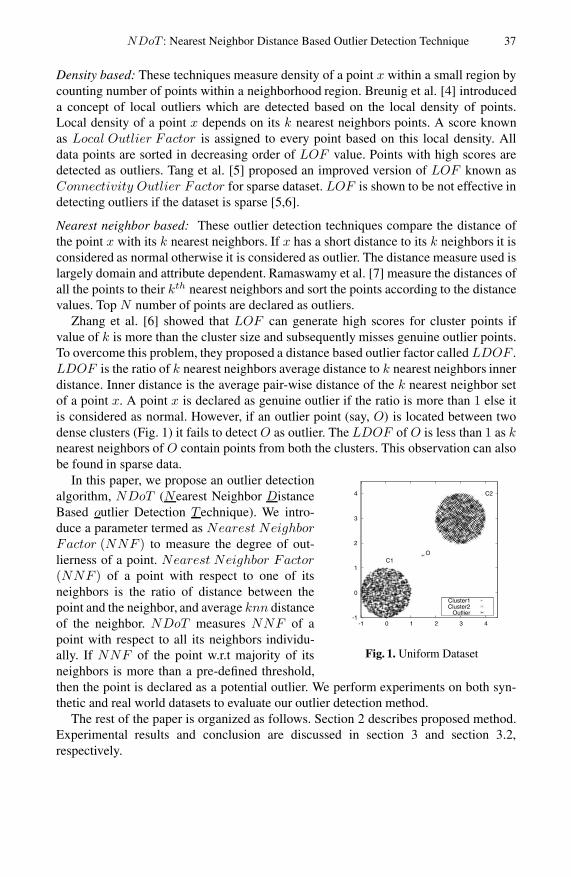
NDoT : Nearest Neighbor Distance Based Outlier Detection Technique 37
Density based: These techniques measure density of a point x within a small region bycounting number of points within a neighborhood region. Breunig et al. [4] introduceda concept of local outliers which are detected based on the local density of points.Local density of a point x depends on its k nearest neighbors points. A score knownas Local Outlier Factor is assigned to every point based on this local density. Alldata points are sorted in decreasing order of LOF value. Points with high scores aredetected as outliers. Tang et al. [5] proposed an improved version of LOF known asConnectivity Outlier Factor for sparse dataset. LOF is shown to be not effective indetecting outliers if the dataset is sparse [5,6].
Nearest neighbor based: These outlier detection techniques compare the distance ofthe point x with its k nearest neighbors. If x has a short distance to its k neighbors it isconsidered as normal otherwise it is considered as outlier. The distance measure used islargely domain and attribute dependent. Ramaswamy et al. [7] measure the distances ofall the points to their kth nearest neighbors and sort the points according to the distancevalues. Top N number of points are declared as outliers.
Zhang et al. [6] showed that LOF can generate high scores for cluster points ifvalue of k is more than the cluster size and subsequently misses genuine outlier points.To overcome this problem, they proposed a distance based outlier factor called LDOF .LDOF is the ratio of k nearest neighbors average distance to k nearest neighbors innerdistance. Inner distance is the average pair-wise distance of the k nearest neighbor setof a point x. A point x is declared as genuine outlier if the ratio is more than 1 else itis considered as normal. However, if an outlier point (say, O) is located between twodense clusters (Fig. 1) it fails to detect O as outlier. The LDOF of O is less than 1 as knearest neighbors of O contain points from both the clusters. This observation can alsobe found in sparse data.
-1
0
1
2
3
4
-1 0 1 2 3 4
OC1
C2
Cluster1Cluster2
Outlier
Fig. 1. Uniform Dataset
In this paper, we propose an outlier detectionalgorithm, NDoT (Nearest Neighbor DistanceBased outlier Detection T echnique). We intro-duce a parameter termed as Nearest NeighborFactor (NNF ) to measure the degree of out-lierness of a point. Nearest Neighbor Factor(NNF ) of a point with respect to one of itsneighbors is the ratio of distance between thepoint and the neighbor, and average knn distanceof the neighbor. NDoT measures NNF of apoint with respect to all its neighbors individu-ally. If NNF of the point w.r.t majority of itsneighbors is more than a pre-defined threshold,then the point is declared as a potential outlier. We perform experiments on both syn-thetic and real world datasets to evaluate our outlier detection method.
The rest of the paper is organized as follows. Section 2 describes proposed method.Experimental results and conclusion are discussed in section 3 and section 3.2,respectively.

38 N. Hubballi, B.K. Patra, and S. Nandi
Average knn distance (x)
NN4(x) = q1, q2, q3, q4, q5
q5x
q4
q3
q1q2
NNk(q2)
Fig. 2. The k nearest neighbor of x with k = 4
2 Proposed Outlier Detection Technique : NDoT
In this section, we develop a formal definition for Nearest Neighbor Factor (NNF )and describe the proposed outlier detection algorithm, NDoT.
Definition 1 (k Nearest Neighbor (knn)Set). Let D be a dataset and x be a pointin D. For a natural number k and a distance function d, a set NNk(x) = q ∈D|d(x, q) ≤ d(x, q
′), q
′ ∈ D is called knn of x if the following two conditions hold.
1. |NNk| > k if q′
is not unique in D or |NNk| = k, otherwise.
2. |NNk \ N q′| = k − 1, where N q
′is the set of all q
′point(s).
Definition 2 (Average knn distance). Let NNk be the knn of a point x ∈ D.Average knn distance of x is the average of distances between x and q ∈ NNk.i.e.
Average knn distance (x) =∑
q d(x, q| q ∈ NNk)/|NNk|Average knn distance of a point x is the average of distances between x and its knn.If Average knn distance of x is less compared to other point y, it indicates that x’sneighborhood region is more densed compared to the region where y resides.
Definition 3 (Nearest Neighbor Factor (NNF )). Let x be a point in D andNNk(x) be the knn of x. The NNF of x with respect to q ∈ NNk(x) is the ratioof d(x, q) and Average knn distance of q.
NNF (x, q) = d(x, q)/Average knn distance(q) (1)
The NNF of x with respect to one of its nearest neighbors is the ratio of distance be-tween x and the neighbor, and Average knn distance of that neighbor. The proposedmethod NDoT calculates NNF of each point with respect to all of its knn and uses avoting mechanism to decide whether a point is outlier or not.
Algorithm 1 describes steps involved in NDoT . Given a dataset D, it calculates knnand Average knn distance for all points in D. In the next step, it computes NearestNeighbor Factor for all points in the dataset using the previously calculated knn andAverage knn distance. NDoT decides whether x is an outlier or not based on a vot-ing mechanism. Votes are counted based on the generated NNF values with respect to

NDoT : Nearest Neighbor Distance Based Outlier Detection Technique 39
Algorithm 1. NDoT (D, k)for each x ∈ D do
Calculate knn Set NNk(x) of x.Calculate Average knn distance of x.
end forfor each x ∈ D do
Vcount = 0 /*Vcount counts number of votes for x being an outlier */for each q ∈ NNk(x) do
if NNF (x, q) ≥ δ thenVcount = Vcount + 1
end ifend forif Vcount ≥ 2
3× |NNk(x)| then
Output x as an outlier in D.end if
end for
all of its k nearest neighbors. If NNF (x, q | q ∈ NNk(x)) is more than a thresholdδ ( in experiments δ = 1.5 is considered), x is considered as outlier with respect to q.Subsequently, a vote is counted for x being an outlier point. If the number of votes are atleast 2/3 of the number of nearest neighbors then x is declared as an outlier, otherwisex is a normal point.
Complexity Time and space requirements of NDoT are as follows.
1. Finding knn set and Average knn distance of all points takes time of O(n2), wheren is the size of the dataset. The space requirement of the step is O(n).
2. Deciding a point x to be outlier or not takes time O(|NNk(x)|) = O(k). For wholedataset the step takes time of O(nk) = O(n), as k is a small constant.
Thus the overall time and space requirements are O(n2) and O(n), respectively.
3 Experimental Evaluations
In this section, we describe experimental results on different datasets. We used two syn-thetic and two real world datsets in our experiments. We also compared our results withclassical LOF algorithm and also with one of its recent enhancement LDOF . Resultsdemonstrate that NDoT outperforms both LOF and LDOF on synthetic datasets. Wemeasure the Recall given by Equation 2 as an evaluation metric. Recall measures howmany genuine outliers are there among the outliers detected by the algorithm. BothLDOF and LOF are of top N style algorithms. For a chosen value of N , LDOF andLOF consider N highest scored points as outliers. However, NDoT makes a binarydecision about a point as either an outlier or normal. In order to compare our algorithmwith LDOF and LOF we used different values of N.
Recall = TP/(TP + FN) (2)

40 N. Hubballi, B.K. Patra, and S. Nandi
where TP is number of true positive cases and FN is the number of false negativecases. It is to be noted that top N style algorithms select highest scored N points asoutliers. Therefore, remaining N -TP are false positive (FP ) cases. As FP can beinferred based on the values of N and TP we do not explicitly report them for LDOFand LOF .
3.1 Synthetic Datasets
-1
0
1
2
3
4
5
-1 0 1 2 3 4 5
Cluster1Cluster2
Outlier
Fig. 3. Circular dataset
There are two synthetic datasets designed toevaluate the detection ability (Recall) of algo-rithms. These two experiments are briefed subse-quently.
Uniform dataset. Uniform distribution dataset isa two dimensional synthetic dataset of size 3139..It has two circular shaped clusters filled withhighly densed points. There is a single outlier(say O) placed exactly in the middle of the twodensed clusters as shown in the Figure 1. We ranour algorithm along with LOF and LDOF onthis dataset and measured the Recall for all thethree algorithms. Obtained results for differentvalues of k are tabulated in Table 1. This tableshows that, NDoT and LOF could detect the single outlier consistently while LDOFfailed to detect it. In case of LDOF the point O has knn set from both the clusters, thusthe average inner distance is much higher than the average knn distance. This results ina LDOF value less than 1. However, NNF value of O is more than 1.5 with respectto all its neighbors q ∈ C1 or C2. Because, q’s average knn distance is much smallerthan the distance between O and q.
Table 1 shows the Recall for all the three algorithms and also the false positivesfor NDoT (while the number of false positives for LDOF and LOF are implicit).It can be noted that, for any dataset of this nature NDoT outperforms the other twoalgorithms in terms of number of false positive cases detected.
Circular dataset. This dataset has two hollow circular shaped clusters with 1000 pointsin each of the clusters. Four outliers are placed as shown in Figure 3. There are twooutliers exactly at the centers of two circles and other two are outside.
The results on this dataset for the three algorithms are shown in the Table 2. Again wenotice both NDoT and LOF consistently detect all the four outliers for all the k valueswhile LDOF fails to detect them. Similar reasons raised for the previous experimentscan be attributed to the poor performance of LDOF .

NDoT : Nearest Neighbor Distance Based Outlier Detection Technique 41
Table 1. Recall comparison for uniform dataset
k Value NDoT LDOF LOFRecall FP Top 25 Top 50 Top 100 Top 25 Top 50 Top 100
5 100.00% 47 00.00% 00.00% 00.00% 100.00% 100.00% 100.00%9 100.00% 21 00.00% 00.00% 00.00% 100.00% 100.00% 100.00%
21 100.00% 2 00.00% 00.00% 00.00% 100.00% 100.00% 100.00%29 100.00% 0 00.00% 00.00% 00.00% 100.00% 100.00% 100.00%35 100.00% 0 00.00% 00.00% 00.00% 100.00% 100.00% 100.00%51 100.00% 0 00.00% 00.00% 00.00% 100.00% 100.00% 100.00%65 100.00% 0 00.00% 00.00% 00.00% 100.00% 100.00% 100.00%
Table 2. Recall comparison for circular dataset with 4 outliers
k Value NDoT LDOF LOFRecall FP Top 25 Top 50 Top 100 Top 25 Top 50 Top 100
5 100.00% 0 50.00% 100.00% 100.00% 100.00% 100.00% 100.00%9 100.00% 0 25.00% 75.00% 100.00% 100.00% 100.00% 100.00%
15 100.00% 10 25.00% 75.00% 100.00% 100.00% 100.00% 100.00%21 100.00% 10 25.00% 50.00% 100.00% 100.00% 100.00% 100.00%29 100.00% 10 25.00% 50.00% 100.00% 100.00% 100.00% 100.00%
3.2 Real World Datasets
In this section, we describe experiments on two realworld datasets taken from UCI ma-chine learning repository. Experimental results are elaborated subsequently.
Shuttle dataset. This dataset has 9 real valued attributes with 58000 instances dis-tributed across 7 classes. In our experiments, we picked the test dataset and used classlabel 2 which has only 13 instances as outliers and remaining all instances as normal.In this experiment, we performed three-fold cross validation by injecting 5 out of 13 in-stances as outliers into randomly selected 1000 instances of the normal dataset. Resultsobtained by the three algorithms are shown in Table 3. It can be observed that NDoT ’sperformance is consistently better than LDOF and is comparable to LOF .
Table 3. Recall Comparison for Shuttle Dataset
k Value NDoT LDOF LOFTop 25 Top 50 Top 100 Top 25 Top 50 Top 100
5 80.00% 20.00% 20.00% 26.66% 26.66% 53.33% 66.66%9 93.33% 26.66% 33.33% 33.33% 06.66% 26.66% 93.33%
15 100.00% 20.00% 33.33% 53.33% 00.00% 26.66% 100.00%21 100.00% 20.00% 33.33% 66.66% 00.00% 26.66% 80.00%35 100.00% 40.00% 73.33% 73.33% 00.00% 20.00% 53.33%
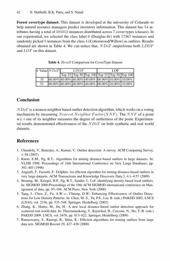
42 N. Hubballi, B.K. Patra, and S. Nandi
Forest covertype dataset. This dataset is developed at the university of Colarado tohelp natural resource managers predict inventory information. This dataset has 54 at-tributes having a total of 581012 instances distributed across 7 cover types (classes). Inour experiential, we selected the class label 6 (Douglas-fir) with 17367 instances andrandomly picked 5 instances from the class 4 (Cottonwood/Willow) as outliers. Resultsobtained are shown in Table 4. We can notice that, NDoT outperforms both LDOFand LOF on this dataset.
Table 4. Recall Comparison for CoverType Dataset
k Value NDoT LDOF LOFTop 25 Top 50 Top 100 Top 25 Top 50 Top 100
35 60.00% 40.00% 40.00% 40.00% 00.00% 10.00% 10.00%51 80.00% 40.00% 40.00% 40.00% 00.00% 10.00% 10.00%
Conclusion
NDoT is a nearest neighbor based outlier detection algorithm, which works on a votingmechanism by measuring Nearest Neighbor Factor(NNF ). The NNF of a pointw.r. t one of its neighbor measures the degree of outlierness of the point. Experimen-tal results demonstrated effectiveness of the NDoT on both synthetic and real worlddatasets.
References
1. Chandola, V., Banerjee, A., Kumar, V.: Outlier detection: A survey. ACM Computing Survey,1–58 (2007)
2. Knorr, E.M., Ng, R.T.: Algorithms for mining distance-based outliers in large datasets. In:VLDB 1998: Proceedings of 24th International Conference on Very Large Databases, pp.392–403 (1998)
3. Angiulli, F., Fassetti, F.: Dolphin: An efficient algorithm for mining distance-based outliers invery large datasets. ACM Transactions and Knowledge Discovery Data 3, 4:1–4:57 (2009)
4. Breunig, M., Kriegel, H.P., Ng, R.T., Sander, J.: Lof: identifying density-based local outliers.In: SIGMOD 2000:Proceedings of the 19th ACM SIGMOD international conference on Man-agement of data, pp. 93–104. ACM Press, New York (2000)
5. Tang, J., Chen, Z., Fu, A.W.-c., Cheung, D.W.: Enhancing Effectiveness of Outlier Detec-tions for Low Density Patterns. In: Chen, M.-S., Yu, P.S., Liu, B. (eds.) PAKDD 2002. LNCS(LNAI), vol. 2336, pp. 535–548. Springer, Heidelberg (2002)
6. Zhang, K., Hutter, M., Jin, H.: A new local distance-based outlier detection approach forscattered real-world data. In: Theeramunkong, T., Kijsirikul, B., Cercone, N., Ho, T.-B. (eds.)PAKDD 2009. LNCS, vol. 5476, pp. 813–822. Springer, Heidelberg (2009)
7. Ramaswamy, S., Rastogi, R., Shim, K.: Efficient algorithms for mining outliers from largedata sets. SIGMOD Record 29, 427–438 (2000)
Some Remarks on the Relation between
Annotated Ordered Sets and Pattern Structures
Tim B. Kaiser1 and Stefan E. Schmidt2
1 SAP AG, Walldorf2 Institut fur Algebra, Technische Universitat Dresden
Abstract. We exhibit an intimate connection between the concept ofan annotated ordered set and that of a pattern structure. This enables anexchange of ideas and techniques between both domains.
1 Introduction
Pattern structures were introduced in [KG01] to model information. The useful-ness of annotated ordered sets for similar purposes was studied in [KSJ08]. Here,we compare and relate the two approaches. To keep the article rationably self-contained we recapitulate both concepts. We see how theorems can be movedbetween both domains and fix a theorem from [KG01].
In the first section we will introduce annotated ordered sets. In the secondsection we will outline pattern structures. In the third section we will argue thatpattern structures can be understood as a certain sub-class of annotated orderedsets and review basic constructions and theorems. In the fourth section we willcorrect a theorem about pattern structures and their projections.
The reader is assumed to be knowledgeable about the basics of order theoryand formal concept analysis as can be found in [DP90] and [GW99].
2 Annotated Ordered Sets
Annotated ordered sets were introduced to model taxonomies, e.g. appearing inthe realm of the Gene Ontology.
Definition 1 ((elementary) annotated ordered set). Let P := (P,≤P) bea finite ordered set (poset), let X be a finite set of labels, and let F : X → 2P bean annotation function. Then we call O := (P , X, F ) an annotated ordered setand refer to (X, F ) as an annotation of P. In case P is a (complete) lattice wecall O an annotated (complete) lattice denoted L. If |F (x)| = 1 for all x ∈ X, forconvenience, we regard F as a map from X to P and say that O is elementary.
It is interesting to note that an annotated ordered set (P , X, F ) can be regardedas a formal context with ordered attributes (X,P , FR) since every mappingT : A → 2B can be interpreted as a relation TR ⊆ A×B where xTRy if and onlyif y ∈ T (x). But the concept lattice of this formal context would not yield the
S.O. Kuznetsov et al. (Eds.): PReMI 2011, LNCS 6744, pp. 43–48, 2011.c© Springer-Verlag Berlin Heidelberg 2011
44 T.B. Kaiser and S.E. Schmidt
intended concept lattice representation of the annotated ordered set, since it doesnot express the semantics of annotation in a taxonomy, that is, if we annotatean example to a class in a taxonomy we implicitly mean that it belongs to allthe super-classes of the class it was annotated to. Additionally, modelling theannotated taxonomy as formal context would be rather counter-intuitive.
We describe how an appropriate formal context can be derived from an anno-tated ordered set to produce its concept lattice representation. For an ordered setP := (P,≤P) and node q ∈ P we denote by ↑ q := p ∈ P | q ≤P p the principalfilter of q and dually by ↓ q the principal ideal. Also, for later use, for N ⊆ Plet ↓N q := n ∈ N | n ≤P q and dually ↑N q := n ∈ N | q ≤P n. Given anannotated ordered set O := (P , X, F ) we can construct a formal context KO :=(X, P, I) where we define the relation I ⊆ X × P by xIp :⇐⇒↓ p ∩ F (x) = ∅.
This means that I equals FR ≤P . Note that in the case of an elementaryannotated ordered set the definition of I can be written as xIp :⇐⇒ F (x) ≤ psince F is regarded as mapping to P (instead of 2P ).
The concept lattice of KO will be denoted by BO := (BO,≤BO), where BO :=
B(KO) is the set of formal concepts of the formal context KO [GW99]. BO iscalled the concept lattice representation of the annotated ordered set O.
In case O forms an annotated complete lattice and (A, B) ∈ BO is a formalconcept in BO, we observe that A = BI is the set of all x ∈ X such that
∧B
is an upper bound of F (x). Also, for convenience, for a node p ∈ P denotepI := pI ⊆ X .
3 Pattern Structures
In [KG01] pattern structures are introduced to model information in the realm ofpharmaceutical research. How pattern structures serve to analyze many-valueddata contexts is described in [Ku09].
Definition 2 (pattern structure). Let G be a set, let D := (D,) be a meet-semilattice, and let δ : G → D. Then P := (G,D, δ) is called pattern structureif δ(G) generates a complete subsemilattice (Dδ,)of D. The elements of G arecalled objects and the elements of D are called descriptions or patterns. Theoperation models a similarity operation on the descriptions.
Pattern structures can be represented by the concept lattices of so called repre-sentation contexts. In the following we sketch the construction of representationcontexts as given in [KG01]. First it is important to note that (Dδ ,) is com-plete and therefore, there exists a (unique) operation to make (Dδ,,) intoa complete lattice. This operation (on D) is given by
⊔X :=
c ∈ Dδ | ∀x ∈X : x c. Furthermore, a subset M of D is called -dense for (Dδ,) if anyelement d ∈ Dδ can be recaptured as join of elements N ⊆ M , that is d =
⊔N .
Now (G, M, I) is a representation context for (G,D, δ) if M is -dense for (Dδ,)and I ⊆ G × M is defined as gIm :⇐⇒ δ(g) m.

Annotated Ordered Sets and Pattern Structures 45
4 Basic Connections
On the one hand, given an elementary annotated ordered set O := (P , X, F )we get a pattern structure O := (X,P, F ) if P allows for (finite) meets andF (X) generates a complete subsemilattice of P. On the other hand, given apattern structure P := (G,D, δ) we always get an elementary annotated orderedset (D, G, δ) when considering the meet-semilattice as ordered set via the usualdefinition c d :⇔ c d = c. Therefore, we see that pattern structures are spe-cial cases of annotated ordered sets and we can immediately transfer all resultson annotated ordered sets to pattern structures. When we consider the otherdirection we must be more careful. But let us first compare the constructions offormal contexts for representation in both cases.
For the time being, let us consider a pattern structure P := (G,D, δ) aselementary annotated ordered set and let us build its associated context via theannotated ordered sets method. We get KP := (G, D, I) where I ⊆ G×D is givenby gId :⇔ δ(g) d. It is obvious that D is -dense for Dδ. If we had dualizedthe order upfront the above construction would have yielded a representationcontext for P. Therefore, we can conclude that the method for representationcontext construction for pattern structures generalizes the method for conceptlattice representation for annotated ordered sets in this case. It is important tonote that Theorem 1 in [KG01] implies that the concept lattices of (different)representation contexts for a given pattern structure are isomorphic.
In [KG01], it follows directly from Theorem 1 that (Dδ,) and the conceptlattice of a representation context of the underlying pattern structure are anti-isomorphic. In the following, we exhibit a connection between the concept latticeof a representation context and D, the ordered set of all patterns. For elementaryannotated complete lattices, Theorem 1 in [KSJ08] makes obvious that theirconcept lattice representations are tied to the underlying complete lattices viaadjunctions. We need to generalize this result to pattern structures, since (D,)is not necessarily a complete lattice.
Theorem 1. Let P := (G,D, δ) be a pattern structure, let K := (G, M, I) be arepresentation context, let ϕ : B(K) −→ D, (A, B) → B be a mapping, andlet μ : D −→ B(K), d → (dI , dII) be a mapping. Then (ϕ, μ) forms a dualadjunction (or Galois connection) between the ordered set of patterns D andthe concept lattice (B(K),≤) of (G, M, I). In particular, ϕ is injective and μ issurjective.
Proof. We show that ϕ is injective (the surjectivity of μ follows from the injec-tivity of ϕ). Assume we have two concepts (A, B) and (C, D) which are mappedto the same element, that is, B = D. We will show that (B)I = A fromwhich it follows that (A, B) = (C, D). We have that g ∈ (B)I if and only ifδ(g) B if and only if δ(g) b for all b ∈ B if and only if g ∈ BI .
The pair (ϕ, μ) forms a Galois connection since ϕ(A, B) d ⇐⇒ B d ⇐⇒(B)I ⊇ dI ⇐⇒ (A, B) ≥ (dI , dII) = μ(d) From the above theorem it follows that the concept lattice of a representationcontext is embedded as a closure system into D.

46 T.B. Kaiser and S.E. Schmidt
In [KSJ08], it is investigated what can happen if we fix an ordered set andthen vary the annotations. It turns out that the annotations are in one-to-onecorrespondence with the closure systems in the filter lattice of the ordered set.Clearly, this implies that in the case of pattern structures if a set of patterns ordescriptions together with a similarity operation is given and we vary the anno-tation function δ freely, we can only get a one-to-one correspondence between(elementary) annotations and a certain subset of the closure systems in the ideallattice (the dual of the filter lattice of the ordered set). In the following we willsingle out this subset.
Theorem 2. Let G be a set of objects, and let D := (D,) be a semi-lattice.The elementary annotations are, up to annotational equivalence, in one-to-onecorrespondence to the principally generated closure systems in the ideal latticeof D.
Proof. Given an elementary annotation δ : G → D every xδ is a principalideal in D and an object intent of a formal concept of (G, D, δ ). Since, ingeneral, the intents of all concepts of a formal context are exactly the meets ofthe object intents the annotation induces a principally generated closure systemin the ideal lattice of D.
Given a closure system X ⊆ 2D in the ideal lattice of D generated by theprincipal ideals I ⊆ 2D we can define a corresponding elementary annotationδI : I → D where ↓ i → i.
5 Projections
For pattern structures so called projections where introduced in [KG01] to modelthe process of simplification of the underlying subsumption order. Projectionsare defined as kernel operators1 on the ordered set of patterns or descriptions.The existence of projections can be characterized by the existence of certainrepresentation contexts. We quote Theorem 2 from [KG01]:
For pattern structures P1 := (G,D, δ1) and P2 := (G,D, δ2) the followingtwo conditions are equivalent.(1) There exists a projection π with δ2 = δ1 π.(2) There exist representation contexts (G, M, I) of P1 and
(G, N, I ∩ (G × N)) of P2 with N ⊆ M .
In the proof of the theorem it is claimed that π(d) :=⊔n ∈ N | n d
is a kernel operator on D if (G, N, I) is a representation context of (G,D, δ).Examples 1 shows that condition (2) in Theorem 2 needs to be boosted 2 andExample 2 shows that the above operator used in the proof is not a kerneloperator as claimed.1 Kernel operators on ordered sets are isotone, idempotent, and dually extensive
self-maps.2 Thanks to Jan Frebel for valuable input.

Annotated Ordered Sets and Pattern Structures 47
Example 1. Let D be given by the structure depicted in Figure 1 and let Gi :=g and δi(g) := ai and Mi := 0, c (visualized by the dotted compartment inFigure 1) for i = 1, 2. Note that the carrier set Dδ of the complete sub-semilatticegenerated by δ(G) is given by ai, 1 for i = 1, 2. It is immediate that Mi is -dense regarding δi for i = 1, 2 and that M2 ⊆ M1, but obviously there exists noprojection π with δ2 = δ1 π.
1
a1
c
a2
0
Fig. 1. (2) implies (1) does not hold inTheorem 2
1
a
c
0
Fig. 2. Operator from the proof is not akernel operator
Example 2. Let D be given by the structure depicted in Figure 2 and let G := gand δ(g) := a and M := 0, c (visualized by the dotted compartment in Figure2). Note that the carrier set Dδ of the complete sub-semilattice generated byδ(G) is given by a, 1. It is immediate that M is -dense regarding δ, butπ : D → D : d → m ∈ M | m d is not contractive since π(c) = 1, thus π isnot a kernel operator.
To repair Theorem 2 we additionally require that δ2 is point-wise contained inδ1 in condition (2) and to repair the proof we make the above operator into akernel operator.
Theorem 3. For pattern structures P1 := (G,D, δ1) and P2 := (G,D, δ2) thefollowing two conditions are equivalent.
(1) There exists a projection π with δ2 = δ1 π.(2) We have δ2 δ1 and there exist representation contexts (G, M, I) of P1 and
(G, N, I ∩ (G × N)) of P2 with N ⊆ M .
Proof. “(1) ⇒ (2)”: Since there exists a projection π with δ2 = δ1 π we have ford ∈ D that δ2(d) = δ1 π(d) = π(δ1(d)) which implies δ2(d) δ1(d) since π iscontractive. We construct the two representation contexts. Let M := D and letN := π(D). Obviously, we have N ⊆ M . Since δ2 = δ1 π we get δ2(G) ⊆ π(D).It remains to show that arbitrary meets of elements from δ2(G) can be recoveredfrom N . Assume F ⊆ δ2(G) and let f :=
F . Since δ2(G) ⊆ π(D) and π is
idempotent we have F = π(F ) which yields f =
π(F ). Since kernel operators

48 T.B. Kaiser and S.E. Schmidt
are (completely) meet-preserving we get f =
π(F ) = π(
F ) ∈ π(D). Thatmeans Dδ2 ⊆ π(D) which shows that π(D) is -dense regarding Dδ2 . The relationI of the first representation context is given by gId :⇔ δ1(g) d. If we look atthe relation J of the second representation we see that for d ∈ π(D) we havegJd :⇔ δ2(g) d. But since π is a kernel operator for d ∈ π(D) it follows thatδ2(g) d ⇐⇒ π(δ2(g)) π(d) ⇐⇒ π(δ2(g)) d ⇐⇒ δ1(g) d which yieldsJ = I ∩ (G × π(D)).
“(2) ⇒ (1)”: We define a self-map on D by π(d) := d ⊔n ∈ N | n d = d ⊔ ↓N d. Note that, in general, is not the supremum operationfor D. Therefore, we must be extra-cautious while showing that π is a kerneloperator. It is easy to see that π acts on Dδ2 as the identity since N is -denseregarding Dδ2 . Also, by definition of
⊔, the image of π equals D ∩ Dδ2 . For
showing that π is monotone, we assume that d ≤ d′. We have ↓N d ⊆↓N d′
which implies that c ∈ Dδ | ∀x ∈↓N d′ : x c is a subset of c ∈ Dδ |∀x ∈↓N d : x c and therefore
⊔ ↓N d =c ∈ Dδ | ∀x ∈↓N d : x c
is less or equal than c ∈ Dδ | ∀x ∈↓N d′ : x c =⊔ ↓N d′. This
implies π(d) = d ⊔ ↓N d d ⊔ ↓N d′ = π(d′) as required. Contractivity ofπ is immediate. It remains to show idempotency. It suffices to make sure that↓N π(d) =↓N d. Since π is contractive we have ↓N π(d) ⊆↓N d. Let n ∈ N withn d. Obviously n d ⊔ ↓N d = π(d). We get ↓N π(d) ⊇↓N d which gives↓N π(d) =↓N d. We have shown that π is a kernel operator on D. It remains toshow that δ2 = δ1 π holds. Let g ∈ G and n ∈ N . From condition (2) it followsthat n δ1(g) ⇔ gIn ⇔ g(I ∩ (G × N)n ⇔ n δ2(g). We deduce ⊔ ↓N
δ1(g) = ⊔ ↓N δ2(g). Expanding the definitions and using the above equationswe get π(δ1(g)) = δ1(g)⊔ ↓N δ1(g) = δ1(g)⊔ ↓N δ2(g) = δ1(g) δ2(g). Sincewe assume δ1 δ2 we have δ1(g) δ2(g) = δ2(g) and deduce (δ1 π)(g) = δ2(g)to complete our proof.
References
[DP90] Davey, B.A., Priestly, H.A.: Introduction to Lattices and Order. CambridgeUniversity Press, Cambridge (1990)
[GW99] Ganter, B., Wille, R.: Formal Concept Analysis. Mathematical Foundations.Springer, Berlin Heidelberg New York (1999)
[KSJ08] Kaiser, T.B., Schmidt, S.E., Joslyn, C.A.: Adjusting Annotated Tax-onomies. International Journal of Foundations of Computer Science(IJFCS): Special Issue: Concept Lattices and Their Applications 18(2), 345–358 (2008)
[KG01] Ganter, B., Kuznetsov, S.O.: Pattern Structures and Their Projections. In:Delugach, H.S., Stumme, G. (eds.) ICCS 2001. LNCS (LNAI), vol. 2120,pp. 129–142. Springer, Heidelberg (2001)
[Ku09] Kuznetsov, S.O.: Pattern Structures for Analyzing Complex Data. In: Sakai,H., Chakraborty, M.K., Hassanien, A.E., Sl ezak, D., Zhu, W. (eds.) RSFD-GrC 2009. LNCS, vol. 5908, pp. 33–44. Springer, Heidelberg (2009)

Solving the Structure-Property Problem Using
k-NN Classification
Aleksandr Perevoznikov, Alexey Shestov,Evgenii Permiakov, and Mikhail Kumskov
Lomonosov Moscow State University, Faculty of Mechanics and Mathematics,Department of Computational Mathematics
GSP-1, Leninskie Gory, Moscow, 119991, Russian [email protected],[email protected]
http://www.math.msu.su/department/vychmath/index.html
Abstract. The solution of the ”structure-property” based on the molec-ular graphs descriptors selection with k-NN classifier is proposed. The re-sults of comparing the construction of predictive models using the searchand without it are given. The stability of the classifier function construc-tion quality is tested using the test sample.
Keywords: Pattern Recognition, QSAR, QSPR, k-NN.
1 Introduction
The task of the ”structure-property” problem is to estimate the relationshipbetween the structure of chemical compounds and their properties. Solution ofthis problem can be divided into two stages: choosing the description of moleculargraphs and the construction of the classifying function. structural descriptors(features) [1] - pairs and triples of singular points [2,3] defined on a triangulatedmolecular surface of the compound were selected for description and singularpoints, defined on molecular graphs.The structural character spectrum of themolecular graph represents the number of the molecular fragments repetitionsin a molecular graph by complete enumeration of all pairs, triples, quadruplesof the singular points [1,4,5]. As a result, the number of descriptors obtained isvery large (about 1000 - 10000) and we must choose how to use them. There areseveral approaches: the use of descriptors, principal component analysis [8], theselection of features. Then the classifying function on the base of the k-NN isconstructed.
2 Problem Statement
The task is to develop a method of descriptors selection of based on the k-NNclassifier and compare it with two other approaches, as well as the constructionof the classifier function, we denote it by F. φ(F) - the quality functional, itallows us to determine which function is the best. In our calculations we used 2
S.O. Kuznetsov et al. (Eds.): PReMI 2011, LNCS 6744, pp. 49–53, 2011.c© Springer-Verlag Berlin Heidelberg 2011

50 A. Perevoznikov et al.
types of the φ(F ) - the percentage of correctly classified objects for the molecularsets which have discrete activity and the following formula
φ(F ) = 1 −
n∑i=1
(F (Mi) − Ai)2
n∑i=1
A2i
. (1)
where F(Mi) is the value of the classifying function on the i-th molecule, Ai isactivity of the i-th molecule (numeric expression of the property), N is a numberof molecules, for molecular sets which have a numeric activity value.
3 Building of a Classifying Function Based on k-NN
Let each molecule is compared a point in Euclidean space RM (coordinates arethe descriptors values) and the activity value, such as class number, boilingpoint. Then there are two possible cases:
1. The activity is discrete. Assume for simplicity that should classify moleculesinto two classes (C1, C2), and we have a training set C. In order to determinea class of a new molecule x we need to find the k nearest points to it from C(denote this set as Cx). Let m1 be a number of points from Cx ∩C1, and m2 bea number of points from Cx ∩ C2. If m1 > m2, then the new molecule belongsto the first class, if m2 > m1 the new molecule belongs to the second class.
2. Activity is indiscrete. Suppose we have a training set C. In order to estimatethe activity of a new molecule x we must find the k nearest points to it from Cand take the average of their activities.
More about k-NN method can be found in [7,8].Our classification method is based on the assumption that closely related
molecules have a similar value of the activity, so distant molecules should not beallowed to affect the result. Given this, we found it necessary to use the limitedradius( not to take into account molecules which are located outside the circleof some radius). To determine it we construct a minimal spanning tree for themolecules of the set represented as points in RM and take an average of its edgeslength.
4 Algorithm of Descriptors Selection of Based on thek-NN
The input is a matrix of descriptors. Denote it A. The output is a set of descrip-tors, where φ(F ) has its greatest value. The algorithm consists of four steps:
1. Using the k-NN method we classify molecules on the base of each descriptorof the matrix A. The best n descriptors are selected by the φ(F ) value.
2. For each set of descriptors obtained in the previous step, in turn, we addanother column of the matrix A, classify molecules on the base of this new set,and the best n2 sets of descriptors are selected.

Solving the Structure-Property Problem Using k-NN Classification 51
3. Values of φ, obtained at the second step, compared with the values on thefirst. For those sets that do not improve the quality of the forecast, we assumethat φ = 0. We select the N best sets.
4. If φ= 0 for all sets or the number of descriptors in the set corresponds tothe maximum m, then we end the calculation, otherwise proceed to the secondstep.
This algorithm can handle a matrix with a huge number of descriptors M.We cant use exhaustive search algorithm due to the the large computationalcomplexity 2M . When using the algorithm described above leading term in theevaluation of the complexity is nmN2M , where N is the number of molecules.
5 Results
5.1 The Results on a Set of Amber Odorants
Comparison of the quality of the k-NN classification using the algorithm ofselection of descriptors (method 1) , based on all features (method 2) and basedon factors (method 3) was conducted on a set of amber odorants (low molecularweight compounds with amber scent), consisting of 129 molecules [2].
8 descriptors matrixes were used. The comparison of the classification qualityis given in the table below.
Table 1. The comparison of the methods quality
Method 1 Method 2 Method 31 75.9689 59.6899 59.68992 74.4186 59.6899 60.46513 75.1937 59.6899 63.56584 76.7441 59.6899 59.68995 75.9689 60.1562 61.24036 77.5193 59.6899 60.46517 76.7441 59.6899 61.24038 76.7441 59.6899 61.2403
It can be seen from the table that the quality of the algorithm of descriptorsselection is better then the quality of the algorithm on all features and all factors.The difference is about 15 percents. But the quality of the algorithm based onall factors is better then the quality of the algorithm based on all features. Sothe selection of principal components can improve the quality of the forecast,but some pre-selection of descriptors must be done.
5.2 The Results on a Set of Toxic Compounds
First, let us say a few words about the set. Chemical toxicity can cause a lot ofbiologically hazardous effects such as damage to genes, or even result in death

52 A. Perevoznikov et al.
of man or animals. About 120000 chemical compounds are to be tested in thenext 10 years. This will require up to 45 million laboratory animals. An alter-native is to provide toxicity prediction based on models built on the previouslytested compounds. We studied a set which is divided into two parts. A trainingset consists of 644 molecules and is used for building models and test set(449compounds) - for their review. In total there are 5 different feature spaces. Onthis set the quality of classification was checked, both of them will predict new(not involved in constructing the model) of the molecules. Below is a table withthe results.
Table 2. Comparison of the classification quality on the training and the test sets
Training set Test set1 0,6114 0,61802 0,7441 0,68733 0,7297 0,68864 0,7809 0,80905 0,7852 0,7582
The table shows that in almost all the feature spaces results on the trainingset is better than on the test. This is due to the fact that the features used forconstruction of models are not universal. But, nevertheless, the result did notdeteriorated greatly, and so the model can be used for prediction.
6 Conclusion
An algorithm of molecular graphs descriptors selection based on the k-NN clas-sifier solving the structure-property problem was developed and implemented.Computational experiments have shown that the application of this algorithmcan significantly improve the quality of classification, and the decreasing of thequality on the learning set is not significant. In the future, we plan to improvethe quality of the prediction through the implementation of connection withthe construction of descriptors. The algorithm of molecular graphs descriptorsselection based on the k-NN classifier is fixed, and we vary the parameters ofthe construction of the alphabet descriptors. Structural descriptors are taken,and the initial parameters (denoted by T0) are set. The quality functional φ(T0)is computed. Then consider the set M =T ||T − T0| < ε. maxT∈Mφ(F (T )) isfound. T, where the maximum value is reached, is denoted Tm and the process isrepeated until Tm = T0 . So we can find the best description of molecular graphsfor the algorithm.

Solving the Structure-Property Problem Using k-NN Classification 53
References
1. Kohov, V.A.: The Method of Quantifying the Similarity of Graphs Based on Struc-tural Spectrs. Izvestiya RAN, Technical Cybernetics 5, 143–159 (1994)
2. Svitanko, I.V., Devetyarov, D.A., Tcheboukov, D.E., Dolmat, M.S., Zakharov, A.M.,Grigoryeva, S.S., Chichua, V.T., Ponomareva, L.A., Kumskov, M.I.: QSAR Model-ing on the Basis of 3D Descriptors Representing the Electrostatic Molecular Surface(Ambergris Fragrances). Mendeleev Communications 17(2), 90–91 (2007)
3. Svitanko, I.V., Kumskov, M.I., Tcheboukov, D.E., Dolmat, M.S., Zakharov, A.M.,Ponomareva, L.A., Grigoryeva, S.S., Chichua, V.T.: QSAR Modeling on the Baseof Electrostatic Molecular Surface (Amber Fragrances). In: 16th European Sympo-sium on Quantum Structure-Activity Relationships and Molecular Modelling, Eu-roQSAR, Italy (2007)
4. Kumskov, M.I., Smolenskiy, E.A., Ponomareva, L.A., Mitushev, D.F., Zefirov, N.S.:System of structural descriptors for solving structure-property problem. Reports ofthe Academy of Sciences 336(1), 64–66 (1994)
5. Hurst, T., Heritage, T.: HQSAR - A Highly Predictive QSAR Technique Based onMolecular Holograms. In: 213th ACS National Meeting, San Francisco, CA, CINF019 (1997)
6. Hoffman, B., Cho, S.J., Zheng, W., Wyrick, S., Nicols, D.E., Mailman, R.B., Trop-sha, A.: Quantitative structure-activity relationship modelling of dopamine D[1]antagonists using comparative molecular field analysis, generic algorithms-partialleast-squares, and K nearest neighbour methods. J. Med. Chem. 42, 3217–3226(1999)
7. Zheng, W., Tropsha, A.: Novel variable selection quantitative structure-propertyrelationship approach based on the k-nearest-neighbour principle. J. Chem. Inf.Comput. Sci. 40, 185–194 (2000)
8. Clark, M., Cramer III, R.D., Jones, D.M., Patterson, D.E., Simeroth, P.E.: Com-parative Molecular Field Analysis(CoMFA) Toward Its Use with 3DStructuralDatabases. Tetrahedron Comput. Methodol. 3, 47–59 (1990)

Stable Feature Extraction with the Help of
Stochastic Information Measure
Alexander Lepskiy
Higher School of Economics, Moscow, Russia
Abstract. This article discusses the problem of extraction of such set ofpattern features that is informative and stable with respect of stochasticnoise. This is done through the stochastic information measure.
1 Introduction
In describing of non deterministic system we must take into account the natureof its uncertainty. In pattern recognition uncertainty could have both proba-bilistic nature, that defined by some additive measure, and more ”imprecise”nature, which can be described, for example, by using monotonous nonadditivemeasures. The feature extraction is the important task of pattern recognitionin general and image analyses in particular. This task consists to extraction ofsome minimal set of features or combinations of them from a set of features withgiven informativeness, which would have sufficient integral informativeness in so-lution of given problem of recognition. The are traditional approaches to solvingthis problem, such as correlation analysis (principal components analysis, etc.),discriminant analysis [2].
In this article we concretized the general problem of informative features ex-traction as follows. Suppose that pattern X is defined by ordered set X =x0, ..., xn−1. We call every subset A ∈ 2X a representation of pattern X . Theproblem is to find such representation A that it will be minimal on the one handand it will be near to X on the other hand. Elements in the X may have differentpriorities, in other words, they may have different informativeness. Therefore, wewill establish correspondence between the element x ∈ X and the nonnegativenumber – a feature ω(x), that characterize the importance of the element x forthe representation of pattern X . We will determine the degree of representative-ness of the set A ∈ 2X for pattern X using the set function μ(A) and require fromthe set function μ to satisfy all the axioms of monotonous measure: 1) μ(∅) = 0,μ(X) = 1 (normalization); 2) μ(A) ≤ μ(B) if A ⊆ B, A, B ∈ 2X (monotonicity).In addition the measure μ meets the certain additional conditions related to thespecific task of pattern recognition. We will call such measures monotonous in-formation measures. In [1] information measures were used to set and solve thetask of finding the most minimal informative polygonal representation of thecurve.
In certain tasks of pattern recognition, in particular, in image processing,image analysis and image recognition random nature of image features can be
S.O. Kuznetsov et al. (Eds.): PReMI 2011, LNCS 6744, pp. 54–59, 2011.c© Springer-Verlag Berlin Heidelberg 2011

Stable Feature Extraction with the Help of Stochastic Information Measure 55
caused by some noisy effects. For example, if the pattern is a discrete planecurve that extracted on the image and features are some characteristics of curvepoints (eg, feature is a estimation of curvature in given point of discrete curve[3]), then a random character of features (eg, curvature) is caused by the noiseof image. In this case the expectation E [M(A)] characterize the level of infor-mativeness of represenation A ∈ 2X and the variance σ2 [M(A)] characterize thelevel of stability of representation to noise pattern. Then there is the problemof finding the most stable and informative representation A ∈ 2X of the pat-tern X . The complexity of solutions of this problem will be determined by thedegree of dependence of random features of each other. Stochastic measure ofinformativeness M will be additive measure if the features are independent ran-dom variables. Otherwise, the measure would be nonadditive measure. In thisarticle mentioned task will be discussed and resolved in the case of probabilisticindependence of random features. The case of random dependency of features isinvestigated in [4].
2 The Average Set Function of Information of Pattern
In general case the feature may be depend from all or some elements from therepresentation A on which it calculated i.e. ω(x) = ω(x, A). For example, letX = Γ be a discrete plane close curve: Γ = (gk)n−1
k=0 , gk = xki + ykj, andω(g, A) = ‖g − g+(A)‖, where g+(A) is a point that follows from the pointg in ordered representation A or ω(g, A) = kε [A] (g) is a some estimation ofcurvature of plane discrete curve that is calculated in ε− neighbourhood of pointg [3].
The degree of completeness of representation A ∈ 2X in describing the patternX with respect to feature ω(x) = ω(x, A) may be assigned with the follow setfunction
μ(A) =∑
x∈Aω(x, A)
/∑x∈X
ω(x, X), A ∈ 2X , (1)
which we call averaged set function of information of pattern X (with respectto feature ω). We put μ(A) = 0 if the value ω(x, A) is not defined for set A (inparticular μ(∅) = 0).
Example 1. Let X = Γ be a discrete plane close curve: Γ = (gk)n−1k=0 , gk =
xki+ykj and B = gi1 , ...,gil ⊆ Γ . Also we introduce the set functions μL(B) =
L(B)/L(Γ ) and μS(B) = S(B)/S(Γ ), where L(B) and S(B) are perimeter andsquare correspondingly of figure, that is limited by polygon with vertex in pointsof ordered set B. Then μL and μS are averaged set functions of informationof curve Γ , where ω(g, A) = ‖g − g+(A)‖ for set function μL and ω(g, A) =0.5 |ρO(g) × ρO(g+(A))| for set function μS , ρO(g) is a radius vector of pointg ∈ A with respect to arbitrary point O. Note that μL is a monotonous measure,and μS is a monotonous measure too if the domain bounded by polygons withvertexes in the points of discrete curve Γ is convex.

56 A. Lepskiy
There is a question when the averaged set functions of information will bemonotonous measure? It can be easily shown that follow proposition is true.
Proposition 1. Averaged set functions of information μ on 2X of form (1) area monotonous measure iff μ obeys the following condition
∑
x∈A
(ω(x, A) − ω(x, A ∪ y)) ≤ ω(y, A ∪ y)
for any set A ∈ 2X and y ∈ X\A.
Corollary 1. If ω(x, A) = ω(x, X) for all x ∈ A and A ∈ 2X then set functionμ of form (1) is an additive measure on 2X .
Let A = xi1 , ..., xis , x, xis+1 , ..., xil
⊆ X be a some representation of patternX . We denote Ak,m(x) =
xis−k+1 , ..., xis , x, xis+1 , ..., xis+m
⊆ X , k + m ≤ l.
Corollary 2. Let ω(x, A) = ω(x, Ak,m(x)) for all x ∈ A and A ∈ 2X , |A| >k + m, then set function μ of form (1) is a monotonous measure iff
k−1∑
r=0
(ω(xis−r , A) − ω(xis−r , A ∪ y)) +
m∑
r=1
(ω(xis+r , A) − ω(xis+r , A ∪ y))
≤ ω(y, A ∪ y)for all A ∈ 2X and y ∈ X\A. In particular, let ω(x, A) = ω(x, A0,1(x)) for allx ∈ A and A ∈ 2X , |A| > 1, then set function μ of form (1) is a monotonousmeasure iff ω(x+(A), A) ≤ ω(x+(A), A ∪ y) + ω(y, A ∪ y) for all A ∈ 2X
and y ∈ X\A, where x+(A) is a point that follows from the point x in orderedrepresentation A.
3 The Stochastic Additive Average Information Measure
Let μ be a averaged information measure on 2X of form (1) and ω(x, A) =ω(x, X) = ω(x) for all x ∈ A and A ∈ 2X . In other words the feature value atpoint x does not depend from considered representation. The estimation of curva-ture ω(g, A) = kε [Γ ] (g) in ε- neighbourhood of point g for discrete plane curveΓ = (gk)n−1
k=0 is an example of this feature. Then (see corollary 1) the measureμ(A) =
∑x∈A ω(x)
/∑x∈X ω(x), A ∈ 2X , is an additive measure. We suppose
that feature characteristics will be independence random variables Ω(x), x ∈ X .In this case the value of information measure M(A) =
∑x∈A Ω(x)
/∑x∈X Ω(x)
for fixed set A ∈ 2X will be random variable too. The set function M(A) will bean additive measure for any random event. We considered the example of thissituation. Suppose that discrete plane curve Γ = (gk)n−1
k=0 , gk = xki + ykj wassubjected to additive stochastic noncorrelated noise. In result we get a randomcurve Γ = (Gk)p−1
k=0, Gk = Xki + Ykj, where Xk = xk + ηk, Yk = yk + ξk,ηk, ξk are random noncorrelated variables and E[ηk] = E[ξk] = 0, σ2[ηk] = σ2
x,k,

Stable Feature Extraction with the Help of Stochastic Information Measure 57
σ2[ξk] = σ2y,k. Suppose that there is such basic set B ⊆ Γ for which random
variables Ω(g), g ∈ B, are independent. In this case the feature characteris-tics ω(G) = Ω(g) will be random variables just as the value of measure M(A),A ∈ 2B, is.
Let E [Ω(x)] = mx, σ2 [Ω(x)] = σ2x. We will investigate numerical character-
istics of random additive measure M(A), A ∈ 2X .
3.1 The Numerical Characteristics of Stochastic Additive AverageInformation Measure
Let us find the mathematical expectation of random variable M(A) with a fixedA ∈ 2X . Random variable M(A) is equal to a quotient two random variablesξ =
∑x∈A Ω(x) and η =
∑x∈X Ω(x).
Lemma 1. Let ξ and η be random variables that taking values in the intervalslξ, lη respectively on positive semiaxis and lη ⊆ ((1 − δ)E [η] , (1 + δ)E [η]), lξ ⊆(E [ξ] − δE [η] ,E [ξ] + δE [η]). Then it is valid the following formulas for meanand variance of distribution of ξ
ηrespectively
E[
ξη
]= E[ξ]
E[η] + E[ξ]E3[η]σ
2 [η] − 1E2[η]K [ξ, η] + r1, (2)
σ2[
ξη
]= 1
E2[η]σ2 [ξ] + E2[ξ]
E4[η]σ2 [η] − 2E[ξ]
E3[η]K [ξ, η] + r2, (3)
where K [ξ, η] is a covariation of random variables ξ and η, could meet the certainadditional conditions re i.e. K [ξ, η] = E [(ξ −E [ξ]) (η − E [η])]; r1, r2 are theresiduals that depend on numerical characteristics of ξ and η and |r1| ≤ δ
1−δ ·E[ξ]+E[η]
E3[η]σ2 [η] ≤ E[ξ]+E[η]
(1−δ)E[η]δ3, |r2| ≤ Cδ3.
Let ξ =∑
x∈A Ω(x) and η =∑
x∈X Ω(x). Then K [ξ, η] = K[∑
x∈A Ω(x),∑
y∈X Ω(y)]
=∑
x∈A K [Ω(x), Ω(x)] +∑
x∈A,y∈X|x =y K [Ω(x), Ω(y)]. Becauserandom variables Ω(x), x ∈ X , are independent, K [Ω(x), Ω(y)] = 0 for x = y,and K [Ω(x), Ω(x)] = σ2
x by definition. Hence, K [ξ, η] =∑
x∈A σ2x. Using the
notation S(A) =∑
x∈A mx, D(A) =∑
x∈A σ2x, we can rewrite formulas (2), (3)
for our case as follows
E [M(A)] = S(A)S(X)
+ S(A)S3(X)
D(X) − 1S2(X)
D(A) + r1, (4)
σ2 [M(A)] = S(X)−2S(A)S3(X) D(A) + S2(A)
S4(X)D(X) + r2. (5)
Notice that, σ2 [M(X\A)] = σ2 [1 − M(A)] = σ2 [M(A)] for A ∈ 2X . We willuse formulas (4) and (5) without their residuals. Respective values E [M(A)] =E [M(A)] − r1, σ2 [M(A)] = σ2 [M(A)]− r2 we will call estimations of numericalcharacteristics. The class of random variables
M(A) : A ∈ 2X
satisfies all the
requirements for a finitely additive stochastic measure [5]: 1) E[M2(A)] < ∞ forall A ∈ 2X ; 2) M(A) is an almost probably finitely additive measure.

58 A. Lepskiy
Note that mathematical expectation E [M(A)] define the set function on 2X
and E [M(∅)] = 0, E [M(X)] = 1. Since S(A) and D(A) are additive set functionthen measure E [M(A)] will be additive too.
3.2 Finding of Optimal Stable Pattern Representation
We set a problem of finding such representation B of pattern X , which cardi-nality is less or equal to the given number k ≥ 3 for which the summarizedvariance
∑A⊆B σ2 [M(A)] will be minimal but the sum of squares of mathe-
matical expectations of all representations∑
A⊆B E2 [M(A)] will be maximal.The value of summarized variance characterizes the stability of representationand all its subset to noise level of pattern and it depends also from numberof elements in representation. The more elements in the presentation we have,then the summarized value of variance is greater. We will use mathematicalexpectations of nonnormalized information measures S(A), A ⊆ X , instead ofE [M(A)], A ⊆ X , for simplification of computations. We introduce follow crite-ria: f(X) =
∑A⊆X σ2 [M(A)]
/∑A⊆X S2(A), |X | ≤ k.
Then it is necessary to find such set B, 3 ≤ |B| ≤ k, for which f(B) → min.We simplify function f(B). Let S2(B) =
∑x∈B m2
x, SD(B) =∑
x∈B σ2xmx.
Proposition 2. If feature characteristics of pattern X are independent randomvariables then following equality is true for every B ∈ 2X:
f(B) = 1S4(B)
D(B) − 2S(B)
S2(B)+S2(B)SD(B)
.
Corollary 3. If σ2x = σ2 = const for all x ∈ B then
f(B) = 1S4(B)
|B| − 2S2(B)
S2(B)+S2(B)
σ2.
As S2(B)/|B| ≤ S2(B) ≤ S2(B) then following corollary is true.
Corollary 4. If σ2x = σ2 = const for all x ∈ B then
|B|2−|B|(|B|+1)S4(B)
σ2 ≤ f(B) ≤ |B|−1S4(B)
σ2.
We will use the “inclusion-exclusion“ procedure for finding of optimal represen-tation which minimize the function f(B). We estimate the variation of functionf(B) to the exclusion of element x from B and inclusion of element y ∈ X\B.
Theorem 1. If feature characteristics of pattern X are independent randomvariables then following asymptotic equality
f ((B\x) ∪ y) − f(B) = 1S4(B)
(Q1(B)(my − mx) + σ2
y − σ2x
)+ o(τ),
is true for every x ∈ B and y ∈ X\B, where Q1(B) =2(3S2(B)+5S2(B))(S2(B)+S2(B))2
SD(B)−4
S(B)D(B), τ =√
1S2(B)
(m2
y + m2y
)+ 1
D2(B)
(σ4
x + σ4y
).

Stable Feature Extraction with the Help of Stochastic Information Measure 59
Corollary 5. If σ2x = σ2 = const for all x ∈ X, then for any x ∈ B and
y ∈ X\B we have f ((B\x) ∪ y)−f(B) = Q2(B)σ2 (my − mx)+o(τ), where
Q2(B) = 2S3(B)
(3S2(B)+5S2(B)
(S2(B)+S2(B))2− 2|B|
S2(B)
), Q2(B) < 0 for all B ⊆ X : |B| ≥ 3
and τ =√
1S2(B)
(m2
y + m2y
)+ 1
D2(B)
(σ4
x + σ4y
).
Formulas from theorem 1 and corollary 5 may be use for construction of algo-rithmic procedures for finding of representation B, which minimize the functionf . Let KB(x, y) = Q1(B)(my−mx)+σ2
y−σ2x. The algorithm for finding of repre-
sentation B of cardinality k which minimize the function f (if random variablesΩ(x), x ∈ X , are independent), consist of following steps:
1) we select the set B0 consisting of k elements of pattern X with maximalvalues of informativeness E [Ω(x)] = mx, x ∈ X , as a initial representation;
2) we compute the value Q1(B0) from Theorem 1 and we find (x, y) =argmin KB0(x, y) : x ∈ B, y ∈ X\B, KB0(x, y) < 0, if this pair is exist. ThenB1 = (B0\x)∪ y is a new representation for which f(B1) ≤ f(B0) accuratewithin to small values of second order. This step will be repeating so long as willbe pairs (x, y): KB(x, y) < 0.
If σ2x = σ2 = const for all x ∈ X , then following conclusion follows from
the corollary 5, if we disregard small values: the optimal representation B withcardinality is less or equal k, which minimize the function f will be consist ofelements with the greatest values E [Ω(x)] = mx (on the assumption of randomvariables Ω(x), x ∈ X , are independent).
Acknowledgement. This work was supported by the grants 10-07-00135, 10-07-00478, 11-07-00591 of RFBR (Russian Foundation for Basic Research).
References
[1] Bronevich, A., Lepskiy, A.: Geometrical Fuzzy Measures in Image Processing andPattern Recognition. In: Proc. of the 10th IFSA World Congress, Istanbul, Turkey,pp. 151–154 (2003)
[2] Duda, R.O., Hart, P.E., Stork, D.G.: Pattern Classification and Scene Analysis:Part I Pattern Classification. John Wiley and Sons, Chichester (1998)
[3] Lepskii, A.E.: On Stability of the Center of Masses of the Vector Representationin One Probabilistic Model of Noiseness of an Image Contour. Automation andRemote Control 68, 75–84 (2007)
[4] Lepskiy, A.E.: Application of Stochastic Information Measure in Problem of Find-ing of Optimal Polygonal Curve Representation. In: Proc. of Intern. Conf. PatternRecognition and Image Analysis, Nizhni Novgorod, vol. 1, pp. 397–400 (2008)
[5] Shiryaev, A.N.: Probability (Graduate Texts in Mathematics). Springer, Heidelberg(1995)

S.O. Kuznetsov et al. (Eds.): PReMI 2011, LNCS 6744, pp. 60–65, 2011. © Springer-Verlag Berlin Heidelberg 2011
Wavelet-Based Clustering of Social-Network Users Using Temporal and Activity Profiles
Lipika Dey and Bhakti Gaonkar
Innovation Labs, Tata Consultancy Services, Delhi, India (lipika.dey,bhakti.g)@tcs.com
Abstract. Encouraged by the success of social networking platforms, more and more enterprises are exploring the use of crowd-sourcing as a method for intra-organization knowledge management. There is not much information about their effectiveness though. While there has been some emphasis on studying friend networks, not much emphasis has been given towards understanding other kinds of user behavior like regularity of access or activity. In this paper we present a wavelet-based clustering method to cluster social-network users into different groups based on their temporal behavior and activity profiles. Cluster characterization reveals the underlying user-group characteristics. User data from web and enterprise social-network platforms have been analyzed.
Keywords: Social Network Analysis, Wavelet transformation, Hierarchical K-means clustering.
1 Introduction
Social networking sites like Twitter and Facebook are figuring in an increasingly important way to market researchers due to their astronomically rising user base over a very short time. Efforts are on to tap the content that is generated in these sites to get valuable business insights. There is also an attempt to replicate these platforms within the secure environments of enterprises and motivate employees to engage in similar social interactions. It is expected that these platforms can motivate knowledge and expertise sharing in a more pro-active and effective way. However, these initiatives can only succeed if user participation is considerably steady and continuous, which is not necessarily true. Studies show that though popular social network sites like Twitter have an increasing user base, but there is also a huge attrition rate. Characterization of users based on their temporal behavior and activity profiles can not only help in identifying valuable and active user groups, but also help in improving the effectiveness of such platforms by identifying rare or infrequent users and motivating them to participate more through various incentives. Identifying anomalous behavior can be yet another important application of this.
In this paper, we present an efficient way of clustering users into different groups based on their temporal behavior in social network forums. While there has been a lot of focus on studying user-groups based on content generated by them, not much work exist on analyzing their temporal behavior. We show that wavelet-based analysis can

Wavelet-Based Clustering of Social-Network Users 61
effectively identify different categories of users, whose behaviors can be easily characterized. The rest of the paper is organized as follows. Section 2 surveys related works. Section 3 presents the background of wavelet analysis. The details of our wavelet based clustering algorithm are discussed in Section 4. Section 5 describes the experiments conducted and the results obtained.
2 Survey of Related Work
Wavelet transform being spatial-temporal in nature can capture temporal as well as frequency-based behavior of signals. In [1], a technique based on Discrete Wavelet Transform was proposed to cluster ECG signals. Though wavelet based analytical techniques are very powerful, they have not seen much use in the field of social-network analysis. There have been several earlier attempts to cluster web-site users into different groups based on their access patterns. In [2] a novel approach was presented to cluster user profiles based on mass distribution using Dempster-Shafer’s theory. Profile similarity was used to make recommendations, personalize Web sites, and create targeted advertisements. In [3], a trace analysis was conducted to characterize user access to videos over web (VOW). Their analysis revealed interesting discoveries like requests for same video spanned over short span of time and that small number of machines accounted for large number of overall requests. In [4], a very recent work, it has been shown how content popularity grows and fades over time in Twitter. In order to uncover the temporal dynamics of online content this has been formulated as time series clustering problem using a similarity metric that is invariant to scaling and shifting. K-Spectral Centroid (K-SC) clustering algorithm is proposed, that can effectively find cluster centroids with their similarity measure applied on wavelet coefficients of the time series.
3 Brief Overview of Wavelet Analysis and Wavelet Transformation
Wavelets are mathematical functions that are very useful in representing data due to various properties like compact support, vanishing moments, dilating relations etc. [5, 6, 7]. Compact support guarantees the localization of wavelets, while vanishing moment guarantees that wavelet processing can distinguish the essential information from non-essential information. These features including facilities for hierarchical representation and manipulation make wavelets a very powerful tool. Wavelet transforms are spatial-temporal in nature. They capture the time as well as the frequency of the signals. In wavelet analysis, the scale that is used to look at data plays a special role.
The Discrete Wavelet Transform can be described as a series of filtering and sub sampling. In each level in this series, a set of 2j−1 coefficients are calculated, where j < J is the scale and N = 2J is the number of samples in the input signal. The coefficients are calculated by applying a high-pass wavelet filter to the signal and down-sampling the result by a factor of 2. At the same level, a low-pass scale filtering is also performed (followed by down-sampling) to produce the signal for the next
62 L. Dey and B. Gaonkar
level. Each set of scale-coefficient corresponds to a “smoothing” of the signal and the removal of details, whereas the wavelet-coefficients correspond to the “differences” between the scales.
Given a signal f having dimension D , low frequency filter L and a high frequency filter H, the Fast wavelet transformation of the signal is computed as follows:
1. Apply H to f, returning a new signal f ,with a domain half the size of D , 2. Similarly, apply L to f, returning another new signal f ,with a domain half the size
of D , 3. If size of D is 2, then return [f , f ] 4. Apply Wavelet transform (recursively) on f , 5. Return f concatenated with the result.
The resultant transformed signal f is Lf , Hf , Hf , … , Hf where Lf is the wavelet coefficient of signal f at the (coarsest) level. It contains the approximated information about original signal. Hf are the wavelet coefficients of the signal at level containing the detailed information of the signal at that level.
The simplest wavelet transformation function is Haar transform which has a single vanishing moment. Haar transform performs an average and difference on a pair of value. We have used Daubechies2 wavelet transforms having two vanishing moments. The corresponding low-level and high-level filters are given by (0.12940952, 0.22414386,-0.8365163, 0.4829629) and (0.4829629, 0.8365163, 0.22414386, -0.12940952) respectively.
4 Wavelet-Based Clustering of User Interaction Data
We assume that user interaction data is represented as a time-series, which records the activity of the user at regular time-intervals. Measure of activity in a given time interval is the number of times the user repeats the activity in that period. Activity definition depends on the type of social network and may include actions like asking a question or answering one, sending messages or tweets, or simply updating status.
Grouping users based on their behavior is performed in two phases. In phase I, Fast Daubechies Transform is applied to the time series data. This transformation yields a set of values that are linear combinations of the original elements of the time series. As mentioned earlier, the coarsest level coefficients obtained with the transformation can provide approximate information about the users, while at each higher level more detailed information about the behavior can be captured. In phase II, we exploit this property of wavelet coefficients to refine the process of clustering repeatedly and obtain more refined and homogeneous groups.
The hierarchical clustering algorithm has been designed based on k-means. Initially, the coefficients obtained at the coarsest level are segregated into k clusters. Phases II is repeated for each new cluster, till the most detailed coefficients are taken into account. The clustering process is summarized below

Wavelet-Based Clustering of Social-Network Users 63
Wavelet based Hierarchical Clustering Algorithm
Let n denote the number of users and m denote the number of time-intervals considered
Input: Set of signals n , , i1, 2 … n and j 1, 2 … . m. Since m should be a power of 2, let m = 2s. Extra fields in the signal, if needed, are padded with zeroes.
• Parameters k1, k2,…,ks, where kt is the number of clusters to be created during the tth iteration.
• Output: p clusters, where p = k1*k2*…*km
1. Apply Fast Daubechies Transform ( ) on each element un of n. The data set is transformed to ,
where ,
2. Assign C
3. For , 1, …, For c=1,2,…,k1*k2*…*ks-1-t
a. Apply K-means clustering on set of elements belonging to C considering only level coefficients of the elements wn belonging to C ,dividing each cluster into kt clusters.
b. As a result of step a. k1*k2*…*kt are formed.
5 Experiments and Results
Several experiments were conducted to study users of different types of social networks. The first and second dataset comprise of Twitter users for a period of one month in 2009 and fifteen days in 2010 respectively. The third and fourth datasets comprise data from an Enterprise Social Network Portal (ESNP) where users ask questions or answer questions posted by other users. It consists of employees and their monthly behavior over 25 months from April 2008 to April 2010. The Twitter data time-series contain the number of tweets sent by each user on the different days. The Enterprise data contains number or questions or answers posted by users in a given month. Table 1 presents details of the datasets as well as the results obtained.
It can be observed from Table 1 that the distributions are identical with one large cluster receiving majority of the data points. It is found that the major cluster always contains infrequent users with low activity profiles. This cluster emerges at the end of first level itself, and remains unchanged through the next iterations. Figure 1 shows the clusters formed for the different datasets after the first level of clustering, i.e. at the coarsest level of approximation. These plots have been generated using total activity during the period. The last column of Table 1 shows that the percentage of users exhibiting significant volumes of activity and continuous presence is very low.

64 L. Dey and B. Gaonk
Table 1
Dataset Number of users
Twitter I 200000 Twitter II 44895
ESNP Answers
21420
ESNP Question
19810
Fig. 1. [a] Twitter data I
Figures 2[a] and 2[b] sho(red dots) and one minor cdata sets respectively. In figactivity of 2 tweets and an Blue dots in the figure detweets and an average preslow-profile users with an avmonths, over the period of profile users with an averagmonths. Figure 2c analysediscussed later.
Fig. 2. Inactive and most acCategory distribution of conten
It is obvious that majorilow profile. Analysis of T
kar
1. Details of Datasets and Clustering results
Time Period
Clusters (#)
% users in largest cluster
% users wihigh-activity
31 days 48 54 0.16 16 days 16 63 0.27 25 months 32 93 0.47
25 months 32 78 0.35
[b] Twitter data II [c] ESNP Answers [d] ESNP Questions
ow activity profiles of sample users from the major cluluster (blue dots) from second Twitter and ESNP answgure 2[a], red dots depict low-profile users with an aver average presence of 1.6 days over the period of 16 da
epict highly active users with an average activity of sence of 12 days. Similarly in figure 2[b], red dots depverage activity of 2.7 answers and an average presence of twenty five months. Blue dots in the figure present hige activity of 30.7 answers and an average presence of 1es the content of ESNP high activity users and will
ctive users [a] Second Twitter dataset [b] ESNP answers nt posted by most active ESNP users
ity of social network users are not regular and maintaiwitter user profiles further reveal that users with high
ith y
uster wers rage ays. 4.5 pict of 3 igh-11.2 l be
[c]
in a hest

Wavelet-Based Clustering of Social-Network Users 65
levels of activity are almost always news groups. In both the datasets, the most active group consisted of IDs of global news agencies like breaking news and TOInews, while the second most active set of users included regional news agencies like AtlantaNews, TOIMumbai, TOIDelhi etc. It is interesting to observe that the patterns of users and usage have remained same over the years, in spite of growing number of users. Further, analysis of ESNP data showed that around 57% of users who logged into the network on any given month, did not do so the very next month. Since very few users take an active role on a continuous basis, the purpose of such networks may not be fulfilled.
The ESNP data used for this experiment had user-given category tags Technology, Programming Languages, HR, Finance, Fun and Entertainment etc. associated to the content. Figure 2c shows that bulk of content contributed by the most active users belong to the Fun and Entertainment category. The other popular categories are culture and Work Life balance. Thus it can be concluded that social networks are positively contributing towards employee bonding. But more can be done to make social networks a platform for enterprise knowledge sharing effectively.
6 Conclusions
In this paper we have explored the temporal behavior of users in social network. We have proposed an effective way of clustering users into different groups and characterized them. It is found that majority of users in any social network are low-profile and irregular. Within enterprise, active interaction is mostly restricted to non-technical content. Schemes to engage users effectively are also essential. Introduction of proper incentives are needed to make social network a viable platform for knowledge sharing. Further work is being carried on to analyze the content and its effectiveness for enterprise.
References
1. Ramakrishnan, A.G., Saha, S.: ECG coding by wavelet-based linear prediction. IEEE Trans. on Biomedical Engineering 44, 1253–1261 (1997)
2. Acharya, S., Smith, B., Parnes, P.: Characterizing User Access to videos on the World Wide Web. In: Proceedings of MMCN (2000)
3. Xie, Y., Phoha, V.V.: Web user clustering from access log using belief function. In: Proceedings of the First International Conference on Knowledge Capture (K-CAP 2001), pp. 202–208. ACM Press, New York (2001)
4. Yang, J., Leskovec, J.: Patterns of Temporal variation in Online Media 5. Graps, A.: An introduction to Wavelets. IEEE, Los Alamitos (1995) 6. Li, T., Li, Q., Zhu, S., Ogihara, M.: A Survey on wavelet Application in Data Mining.
ACM SIGKDD Exploration Newsletter 4(2) (2002) 7. Daubechies, I.: Ten lectures on Wavelets. SIAM, Philadelphia (1991)
Tight Combinatorial Generalization Bounds
for Threshold Conjunction Rules
Konstantin Vorontsov and Andrey Ivahnenko
Dorodnycin Computing Center RAS, Moscow, RussiaMoscow Institute of Physics and Technology, Moscow, Russia
[email protected], [email protected]
Abstract. We propose a combinatorial technique for obtaining tightdata dependent generalization bounds based on a splitting and connec-tivity graph (SC-graph) of the set of classifiers. We apply this approachto a parametric set of conjunctive rules and propose an algorithm foreffective SC-bound computation. Experiments on 6 data sets from theUCI ML Repository show that SC-bound helps to learn more reliablerule-based classifiers as compositions of less overfitted rules.
Keywords: computational learning theory, generalization bounds, per-mutational probability, splitting-connectivity bounds, rule induction.
1 Introduction
Obtaining exact generalization bounds remains an open problem in Computa-tional Learning Theory [1]. Experiments [8,9] have shown that two fine effectsshould be taken into account simultaneously to obtain exact bounds: the split-ting of the set into error levels and the similarity of classifiers. Many practicallyused sets contain a lot of similar classifiers that differ on one object, they arecalled connected. In this work we develop a combinatorial approach that dealswith splitting and connectivity together and gives tight or even exact boundson probability of overfitting. We apply a new SC (splitting and connectivity)combinatorial bound to the set of conjunctive rules and propose the overfittingreduction method compatible with most usual rule induction engines.
2 Definitions and Notation
Let X = x1, . . . , xL be a set of objects and A be a set of classifiers. A binaryloss function I : A × X → 0, 1 exists such that I(a, x) = 1 if a classifier aproduces an error on an object x. A binary vector (ai) ≡
(I(a, xi)
)Li=1 of size L
is called an error vector of the classifier a. Assume that all classifiers from Ahave pairwise different error vectors. Supported by Russian Foundation for Basic Research grant 11-07-00480 and the
program “Algebraical and combinatorial methods of cybernetics and new generationinformation systems” of Russian Academy of Sciences, Branch of Mathematics.
S.O. Kuznetsov et al. (Eds.): PReMI 2011, LNCS 6744, pp. 66–73, 2011.c© Springer-Verlag Berlin Heidelberg 2011
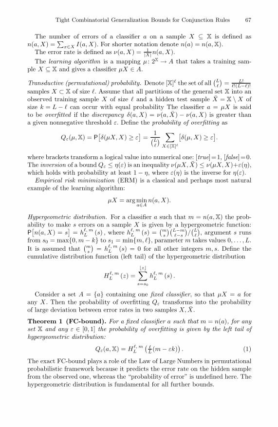
Tight Combinatorial Generalization Bounds for Conjunction Rules 67
The number of errors of a classifier a on a sample X ⊆ X is defined asn(a, X) =
∑x∈X I(a, X). For shorter notation denote n(a) = n(a, X).
The error rate is defined as ν(a, X) = 1|X|n(a, X).
The learning algorithm is a mapping μ : 2X → A that takes a training sam-ple X ⊆ X and gives a classifier μX ∈ A.
Transductive (permutational) probability. Denote [X] the set of all(L
)= L!
!(L−)!
samples X ⊂ X of size . Assume that all partitions of the general set X into anobserved training sample X of size and a hidden test sample X = X \ X ofsize k = L − can occur with equal probability The classifier a = μX is saidto be overfitted if the discrepancy δ(a, X) = ν(a, X) − ν(a, X) is greater thana given nonnegative threshold ε. Define the probability of overfitting as
Qε(μ, X) = P[δ(μX, X) ≥ ε
]=
1(L
)∑
X∈[X]
[δ(μ, X) ≥ ε
].
where brackets transform a logical value into numerical one: [true]=1, [false]=0.The inversion of a bound Qε ≤ η(ε) is an inequality ν(μX, X) ≤ ν(μX, X)+ε(η),which holds with probability at least 1 − η, where ε(η) is the inverse for η(ε).
Empirical risk minimization (ERM) is a classical and perhaps most naturalexample of the learning algorithm:
μX = argmina∈A
n(a, X).
Hypergeometric distribution. For a classifier a such that m = n(a, X) the prob-ability to make s errors on a sample X is given by a hypergeometric function:P[n(a, X) = s
]= h, m
L (s) , where h, mL (s) =
(ms
)(L−m−s
)/(L
), argument s runs
from s0 = max0, m − k to s1 = minm, , parameter m takes values 0, . . . , L.It is assumed that
(ms
)= h, m
L (s) = 0 for all other integers m, s. Define thecumulative distribution function (left tail) of the hypergeometric distribution
H, mL (z) =
z∑
s=s0
h, mL (s) .
Consider a set A = a containing one fixed classifier, so that μX = a forany X . Then the probability of overfitting Qε transforms into the probabilityof large deviation between error rates in two samples X, X.
Theorem 1 (FC-bound). For a fixed classifier a such that m = n(a), for anyset X and any ε ∈ [0, 1] the probability of overfitting is given by the left tail ofhypergeometric distribution:
Qε(a, X) = H, mL
(L
(m − εk)). (1)
The exact FC-bound plays a role of the Law of Large Numbers in permutationalprobabilistic framework because it predicts the error rate on the hidden samplefrom the observed one, whereas the “probability of error” is undefined here. Thehypergeometric distribution is fundamental for all further bounds.

68 K. Vorontsov and A. Ivahnenko
Theorem 2 (VC-bound). For any set X, any learning algorithm μ, and anyε ∈ [0, 1] the probability of overfitting is bounded by the sum of FC-bounds over A:
Qε(μ, X) ≤∑
a∈A
H, mL
(L(m − εk)
), m = n(a). (2)
Further weakening this bound gives a well known form of the VC-bound:Qε(μ, X) ≤ |A|max
mH, m
L
(L (m − εk)
) ≤ |A| · 32e−ε2 for a case = k.
VC-bound is highly overestimated because all classifiers make approximatelyequal contributions to the VC-bound. However, the set of classifiers is usuallysplit into error rates in quite nonuniform manner. Most classifiers are unsuit-able, have vanishing probability to be obtained as a result of learning and makea negligible contribution to the probability of overfitting. On the other hand,similar classifiers share their contribution, thus each of them contributes poorlyagain. VC theory totally ignores both advantageous effects.
3 Splitting and Connectivity Bounds
Define the order relation on classifiers a ≤ b as a natural order on their error vec-tors: ai ≤ bi for all i = 1, . . . , L. Introduce Hamming distance between error vec-tors: ρ(a, b) =
∑Li=1 |ai−bi|. Classifiers a and b are called connected if ρ(a, b) = 1.
Define the precedence relation on classifiers a ≺ b as(a ≤ b
) ∧ (ρ(a, b) = 1
).
The set of classifiers A can be represented by a multipartite directed graphthat we call the splitting and connectivity graph (SC-graph) in which verticesare classifiers, and edges (a, b) are pairs of classifiers such that a ≺ b. Partitesubsets Am = a ∈ A : n(a) = m are called error layers, m = 0, . . . , L. Eachedge of the SC-graph (a, b) can be uniquely labeled by an object xab ∈ X suchthat I(a, xab) = 0 and I(b, xab) = 1.
Upper connectivity q(a) = #xab ∈ X
∣∣ a ≺ b
of a classifier a is the numberof edges leaving the vertex a.
Inferiority r(a) = #xbc ∈ X
∣∣ b ≺ c ≤ a
of a classifier a is the number ofdifferent objects assigned to edges below the vertex a in the SC-graph. If a correctclassifier a0 ∈ A exists such that n(a0) = 0 then inferiority is equal to the numberof errors, r(a) = n(a). In general case r(a) ≤ n(a).
Theorem 3 (SC-bound). If μ is ERM then for any ε ∈ [0, 1] the probabilityof overfitting is bounded by the weighted sum of FC-bounds over the set A:
Qε(μ, X) ≤∑
a∈A
PaH−q, m−rL−q−r
(L(m − εk)
), (3)
where q = q(a) is upper connectivity, r = r(a) is inferiority, m = n(a) is thenumber of errors of classifier a, Pa =
(L−q−r
−q
)/(L
)is an upper bound on the
probability to learn the classifier a, P[μX =a] ≤ Pa.
The weight Pa decreases exponentially as connectivity q(a) and inferiority r(a)increase. This fact has two important consequences.

Tight Combinatorial Generalization Bounds for Conjunction Rules 69
First, connected sets of classifiers are less subjected to overfitting. Not onlythe fact of connectedness but better the number of connections is important.
Second, only lower layers contribute significantly to the probability of overfit-ting. This fact encourages effective procedures for SC-bound computation.
SC-bound (3) is much more tight than the VC-bound (2). It transforms tothe VC-bound by substituting q = r = 0, i. e. by disregarding the SC-graph.
4 SC-Bound for Threshold Conjunctive Rules
Consider a classification problem with labels yi ∈ Y , i = 1, . . . , L assigned toeach object xi ∈ X respectively. Consider a parametric set R of conjunctive rules
r(x; θ) =∏
j∈J
[xj ≤ θj
],
where x=(x1, . . . , xn) is a vector of numerical features of object x, J ⊆ 1, . . . , nis a subset of features, θj ∈ R is a threshold parameter for j-th feature. An ob-ject x is said to be covered by the rule r(x) if r(x) = 1.
A rule induction system learns a rule set Ry for each class y ∈ Y from a trainingset X . Two criteria are optimized simultaneously to select useful rules — thenumber of positive and negative examples covered by r, respectively:
p(r, X) = #xi ∈ X
∣∣ r(xi) = 1, yi = y → max;
n(r, X) = #xi ∈ X
∣∣ r(xi) = 1, yi = y → min .
In practice the two-criteria optimization task is reduced to one-criterion taskby means of heuristic function H(p, n). Examples of H are Fisher’s exact test [5],entropy, Gini index, χ2- and ω2-tests, and many others [4].
Rule based classifier. After learning the rule sets Ry for all y ∈ Y the classifiercan be buildup as a composition of rules, e.g. as a weighted voting:
a(x) = argmaxy∈Y
∑
r∈Ry
wrr(x),
where weights wr ≥ 0 are learned from the training set X . So, there are threethings to learn: (1) thresholds θj , j ∈ J for each subset J ; (2) feature subset Jfor each rule r; (3) weight wr for each rule r. Respectively, there are three reasonsfor overfitting. In this work we use SC-bound to estimate overfitting resultingfrom thresholds learning and build a criterion for feature subset selection, withmotivation that a good classifier can be hardly build up from overfitted rules.
The idea of heuristic modification is to obtain the SC-bound on p and n for afixed J ; then to get inverted estimates that hold with probability at least 1− η:
1kp(r, X) ≥ 1
p(r, X) − εp(η), 1
kn(r, X) ≤ 1
n(r, X) + εn(η),
and to use them instead of p, n in a heuristic H ′(p, n) = H(p−εp(η), n+εn(η)
).
The modified heuristic H ′ gives a more accurate features selection criterion thattakes into account the overfitting resulting from thresholds learning.
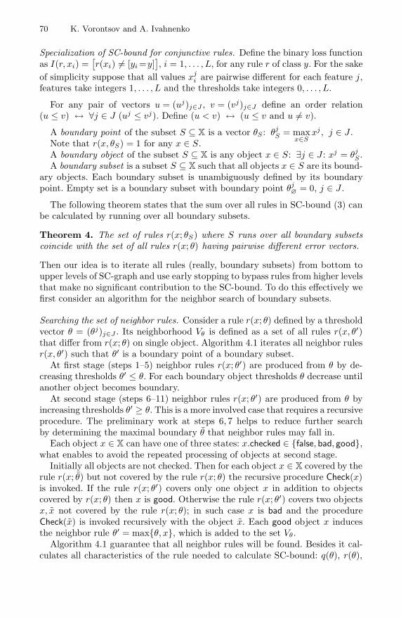
70 K. Vorontsov and A. Ivahnenko
Specialization of SC-bound for conjunctive rules. Define the binary loss functionas I(r, xi) =
[r(xi) = [yi =y]
], i = 1, . . . , L, for any rule r of class y. For the sake
of simplicity suppose that all values xji are pairwise different for each feature j,
features take integers 1, . . . , L and the thresholds take integers 0, . . . , L.
For any pair of vectors u = (uj)j∈J , v = (vj)j∈J define an order relation(u ≤ v) ↔ ∀j ∈ J (uj ≤ vj). Define (u < v) ↔ (u ≤ v and u = v).
A boundary point of the subset S ⊆ X is a vector θS : θjS = max
x∈Sxj , j ∈ J .
Note that r(x, θS) = 1 for any x ∈ S.A boundary object of the subset S ⊆ X is any object x ∈ S: ∃j ∈ J : xj = θj
S .A boundary subset is a subset S ⊆ X such that all objects x ∈ S are its bound-
ary objects. Each boundary subset is unambiguously defined by its boundarypoint. Empty set is a boundary subset with boundary point θj
∅= 0, j ∈ J .
The following theorem states that the sum over all rules in SC-bound (3) canbe calculated by running over all boundary subsets.
Theorem 4. The set of rules r(x; θS) where S runs over all boundary subsetscoincide with the set of all rules r(x; θ) having pairwise different error vectors.
Then our idea is to iterate all rules (really, boundary subsets) from bottom toupper levels of SC-graph and use early stopping to bypass rules from higher levelsthat make no significant contribution to the SC-bound. To do this effectively wefirst consider an algorithm for the neighbor search of boundary subsets.
Searching the set of neighbor rules. Consider a rule r(x; θ) defined by a thresholdvector θ = (θj)j∈J . Its neighborhood Vθ is defined as a set of all rules r(x, θ′)that differ from r(x; θ) on single object. Algorithm 4.1 iterates all neighbor rulesr(x, θ′) such that θ′ is a boundary point of a boundary subset.
At first stage (steps 1–5) neighbor rules r(x; θ′) are produced from θ by de-creasing thresholds θ′ ≤ θ. For each boundary object thresholds θ decrease untilanother object becomes boundary.
At second stage (steps 6–11) neighbor rules r(x; θ′) are produced from θ byincreasing thresholds θ′ ≥ θ. This is a more involved case that requires a recursiveprocedure. The preliminary work at steps 6, 7 helps to reduce further searchby determining the maximal boundary θ that neighbor rules may fall in.
Each object x ∈ X can have one of three states: x.checked ∈ false, bad, good,what enables to avoid the repeated processing of objects at second stage.
Initially all objects are not checked. Then for each object x ∈ X covered by therule r(x; θ) but not covered by the rule r(x; θ) the recursive procedure Check(x)is invoked. If the rule r(x; θ′) covers only one object x in addition to objectscovered by r(x; θ) then x is good. Otherwise the rule r(x; θ′) covers two objectsx, x not covered by the rule r(x; θ); in such case x is bad and the procedureCheck(x) is invoked recursively with the object x. Each good object x inducesthe neighbor rule θ′ = maxθ, x, which is added to the set Vθ.
Algorithm 4.1 guarantee that all neighbor rules will be found. Besides it cal-culates all characteristics of the rule needed to calculate SC-bound: q(θ), r(θ),

Tight Combinatorial Generalization Bounds for Conjunction Rules 71
Algorithm 4.1. Seek the neighborhood Vθ of the rule r(x; θ).Require: features subset J , thresholds θ = (θj)j∈J , class label y ∈ Y , general set X.Ensure: Vθ, Xθ, X ′
θ , q(θ), r(θ), n(θ).
1: Vθ := ∅;2: for all x ∈ X such that r(x; θ) = 1 and θj = xj for some j ∈ J do3: for all j ∈ J such that xj = θj do4: θ′j := max
xj
i
∣∣ xi ∈ X, xi < θ;
5: AddNeighbor(θ, θ′, x);6: for all j ∈ J do7: θj := max
L, xj
∣∣ x ∈ X, xj > θj , xt ≤ θt, t = j;
8: for all j ∈ J do9: for all x such that θj < xj ≤ θj do
10: if x < θ and x.checked = false then11: Check(x);
12: Procedure Check(x)13: for all j ∈ J such that θj < xj do14: for all x such that θj < xj < xj do15: if θ < x < x then16: x.checked := bad;17: if x.checked = false then Check(x);18: exit;19: x.checked := good;20: θ′j := maxθj , xj, for all j ∈ J ;21: AddNeighbor(θ, θ′, x);
22: Procedure AddNeighbor (θ, θ′, xi)23: add the rule θ′ into the set of neighbors Vθ;24: if r(xi; θ) = [yi=y] then25: Xθ := Xθ ∪ xi; q(θ) := |Xθ |;26: else27: X ′
θ := X′θ ∪ X ′
θ′ ∪ xi; r(θ) := |X′θ |; n(θ) := n(θ′) + 1;
and n(θ). To avoid the exhaustive search of all objects at steps 4, 7, 9, 14 thesorting index is to be built in advance for each coordinate j ∈ J .
Level-wise bottom-up calculation of SC-bound. Algorithm 4.2 starts from a lowestlayer of classifiers. At each step it process a layer Θ consisting of all rules θ thatmakes m = n(θ) errors on general set. For each rule θ Algorithm 4.2 calculates itscontribution to the SC-bound, builds its neighborhood, and forms the (m+1)-thlayer Θ′ joining upper parts of all neighborhoods. The steps are repeated untillayer contribution becomes sufficiently small. Note that early stopping givesa lower estimate for (3), witch is upper bound on probability of overfitting.
Experiment. We used following state-of-the art algorithms as baseline rule learn-ers: C4.5 [7], C5.0 [6], RIPPER [2], and SLIPPER [3]. Our rule learning enginewas based on breadth-first search as feature selection strategy and Fisher’s ex-act test (FET) as heuristic H . To build compositions of rules three algorithms

72 K. Vorontsov and A. Ivahnenko
Algorithm 4.2. SC-bound calculation for the set of conjunction rules.Require: features subset J , class label y ∈ Y , set of objects X.Ensure: Qε — SC-bound on probability of overfitting (3).
1: Θ := Arg minθ
n(θ); Qε := 0;
2: repeat3: Qε,m := 0; Θ′ := ∅;4: for all θ ∈ Θ do5: call Algorithm 4.1 to build the neighborhood Vθ;6: Qε,m := Qε,m + 1
CL
C−q(θ)
L−q(θ)−r(θ)H−q(θ), n(θ)−r(θ)
L−q(θ)−r(θ)
(L
(n(θ) − εk));
7: Θ′ := Θ′ ∪ θ′ ∈ Vθ : n(θ′) = n(θ) + 1
;
8: Qε := Qε + Qε,m; Θ := Θ′;9: until the contribution of the m-th layer Qε,m becomes small.
has been implemented. Logistic Regression (LR) is a linear classifier that ag-gregates rules learned independently. Weighted Voting (WV) is a boosting-likeensemble of rules similar to SLIPPER which learns each subsequent rule fromreweighted training set. Decision List (DL) is a greedy algorithm which learnseach subsequent rule from training objects not covered by all previous rules.
We implemented two modifications of heuristic H ′(p, n). The SC modificationuses SC-bound on the probability of overfitting Qε as described above. The MCmodification uses the Monte-Carlo estimation of Qε via 100 random partitionsX = X X. For both modifications we set = k.
Table 1. Experimental results on 6 real data sets from UCI Machine Learning Reposi-tory. For each pair 〈task, algorithm〉 an average testing error obtained from 10-fold crossvalidation is given, in percents. For each task three best results are bold-emphasized.Algorithms 1–7 are baseline rule learners. Our algorithms: WV — Weighted Voting,DL — Decision List, SC — using heuristic modified by SC-bound, MC — usingheuristic modified by Monte-Carlo estimation of the probability of overfitting.
tasksalgorithms
australian echo-card heart dis. hepatitis labor liver
1 RIPPER−opt 15.5 2.9 19.7 20.7 18.0 32.7
2 RIPPER+opt 15.2 5.5 20.1 23.2 18.0 31.3
3 C4.5 (Tree) 14.2 5.5 20.8 18.8 14.7 37.74 C4.5 (Rules) 15.5 6.8 20.0 18.8 14.7 37.5
5 C5.0 14.0 4.3 21.8 20.1 18.4 31.9
6 SLIPPER 15.7 4.3 19.4 17.4 12.3 32.2
7 LR 14.8 4.3 19.9 18.8 14.2 32.0
8 WV 14.9 4.3 20.1 19.0 14.0 32.3
9 DL 15.1 4.5 20.5 19.5 14.7 35.8
10 WV+MC 13.9 3.0 19.5 18.3 13.2 30.7
11 DL+MC 14.5 3.5 19.8 18.7 13.8 32.8
12 WV+SC 14.1 3.2 19.3 18.1 13.4 30.2
13 DL+SC 14.4 3.6 19.5 18.6 13.6 32.3
Tight Combinatorial Generalization Bounds for Conjunction Rules 73
Results are presented in Table 1. Initial unmodified versions of our algorithmsWV and DL with FET heuristic have a performance comparable to the baseline.WV outperforms DL, what corresponds to the results of other authors. Both SCand MC modifications of the FET heuristic reduce overfitting of rules and ofclassifier as a whole. Both modified classifiers outperform their respective initialversions for all 6 tasks. It must be emphasized that the only modification isthe rule evaluation heuristic, all other things being equal. Thus, all differencein performance is due to generalization bound used in modified FET heuristic.The difference between SC and MC results is not significant, but MC estimationis much more time consuming. A moderate looseness of the SC-bound really takesplace but does not reduce its practical usefulness as a rule selection criterion.
5 Conclusion
This work gives a new SC (splitting and connectivity) combinatorial bound onprobability of overfitting. It takes into account a fine internal structure of theset of classifiers formalized in terms of the SC-graph. For a set of threshold con-junctive rules a level-wise bottom-up algorithm with early stopping is proposedfor effective SC-bound computation. The inverted SC-bound is used to mod-ify standard rule evaluation heuristic. This modification can be build in mostknown rule learners. It enables to take into account an amount of overfittingresulting from thresholds learning, and then to select features subset for eachrule more accurately. Experiments on six real data sets show that the proposedmodification reduces overfitting significantly.
References
1. Boucheron, S., Bousquet, O., Lugosi, G.: Theory of classification: A survey of somerecent advances. ESAIM: Probability and Statistics (9), 323–375 (2005)
2. Cohen, W.W.: Fast effective rule induction. In: Proc. of the 12th International Con-ference on Machine Learning, Tahoe City, CA, pp. 115–123. Morgan Kaufmann, SanFrancisco (1995)
3. Cohen, W.W., Singer, Y.: A simple, fast and effective rule learner. In: Proc. of the16 National Conference on Artificial Intelligence, pp. 335–342 (1999)
4. Furnkranz, J., Flach, P.A.: Roc ‘n’ rule learning-towards a better understanding ofcovering algorithms. Machine Learning 58(1), 39–77 (2005)
5. Martin, J.K.: An exact probability metric for decision tree splitting and stopping.Machine Learning 28(2-3), 257–291 (1997)
6. Quinlan, J.R.: C4.5: Programs for machine learning. Morgan Kaufmann, San Fran-cisco (1993)
7. Quinlan, J.R.: Bagging, boosting, and C4.5. AAAI/IAAI 1, 725–730 (1996)8. Vorontsov, K.V.: Combinatorial probability and the tightness of generalization
bounds. Pattern Recognition and Image Analysis 18(2), 243–259 (2008)9. Vorontsov, K.V.: Splitting and similarity phenomena in the sets of classifiers and
their effect on the probability of overfitting. Pattern Recognition and Image Anal-ysis 19(3), 412–420 (2009)

An Improvement of Dissimilarity-Based ClassificationsUsing SIFT Algorithm
Evensen E. Masaki and Sang-Woon Kim
Dept. of Computer Science and Engineering,Myongji University, Yongin, 449-728 South Korea
evenalexjr,[email protected]
Abstract. In dissimilarity-based classifications (DBCs), classifiers are not basedon the feature measurements of individual objects, but rather on a suitable dissim-ilarity measure among the objects. In this paper, we study a new way of measuringthe dissimilarity between two object images using a SIFT (Scale Invariant FeatureTransformation) algorithm [5], which transforms image data into scale-invariantcoordinates relative to local features based on the statistics of gray values in scale-space. With this method, we find an optimal or nearly optimal matching amongdiffering images in scaling and rotation, which leads us to obtain dissimilarityrepresentation after matching them. Our experimental results, obtained with well-known benchmark databases, demonstrate that the proposed mechanism workswell and, compared with the previous approaches, achieves further improved re-sults in terms of classification accuracy.
1 Introduction
Dissimilarity-based classifications (DBCs) [6] are a way of defining classifiers amongclasses; the process is not based on the feature measurements of individual objects, butrather on a suitable dissimilarity measure among them. The problem with this strategyis that we need to measure the inter-pattern dissimilarities for all the training samples toensure there is no zero distance between objects of different classes. Several strategiescan be employed to address this problem, which include the regional distance [1], theEuclidean distances of images [9], a dynamic programming technique [4], and classi-fication of regions of interest (ROIs) [8]. In [9], Wang et al. propose a new Euclideandistance, called IMage Euclidean Distance (IMED). Unlike the traditional one, IMEDtakes into consideration the spatial relationships of pixels. From this point of view, theresearchers claim to get a more reliable similarity measure.
In addition, in [4], Kim and Gao propose a way of measuring the dissimilarity dis-tance between two images of an object when the images have different directions andsizes and there is no direct feature correspondence. In this method, a dynamic program-ming technique, such as dynamic time warping, is used to overcome the limitationsof one-to-one mapping. Recently, in [8], Sorensen et al. proposed a method of directlymeasuring dissimilarities between images by using region of interests (ROIs) of the seg-ments. When computing the dissimilarity between two images, x1 and x2, they consider
This work was supported by the National Research Foundation of Korea funded by the KoreanGovernment (NRF-2011-0002517).
S.O. Kuznetsov et al. (Eds.): PReMI 2011, LNCS 6744, pp. 74–79, 2011.c© Springer-Verlag Berlin Heidelberg 2011

An Improvement of Dissimilarity-Based Classifications Using SIFT Algorithm 75
an associated weight, (x1i, x2j), that expresses the textural dissimilarity between thetwo corresponding ROIs, x1i and x2j . Here, to avoid a case in which all ROIs in x1 arematched to all ROIs in x2, they employ a way of matching every ROI in one image withthe most similar ROI in the other image.
On the other hand, Lowe [5] proposed the scale invariant feature transformation(SIFT) algorithm for extracting distinctive invariant features from images that can beused to perform reliable matching between different views of an object. The features areinvariant to image scale and rotation, and are shown to provide robust matching acrossa substantial range of affine distortion, addition of noise, and change in illumination.Thus, SIFT can be used to detect distinct features in an image and to transform imagedata into scale-invariant coordinates relative to local features. The algorithm consistsof four main steps to generate the set of image features: scale-space peak detection,keypoint localization, orientation assignment, and keypoint descriptor.
The major task of this study is to deal with how dissimilarity measure can be ef-fectively computed. However, when there are many kinds of variations based on suchfactors as pose (direction), scaling, and illumination [1], [3], it is difficult to improvethe performance of DBCs in the dissimilarity space. To overcome this limitation andthereby improve the classification performance of DBCs, in this paper, we study a newway of enriching the representational capability of dissimilarity measures. In particu-lar, this goal can be achieved by using a SIFT algorithm based on the statistics of grayvalues in scale-space. With regard to measuring the dissimilarity of the object images,we prefer not to directly measure the dissimilarity from the images; rather, we employa particular way of using SIFT to adjust or scale the object images. This measure effec-tively serves as a new “feature” component in the dissimilarity space.
2 DBCs with SIFT Algorithm
Scale Invariant Feature Transformation (SIFT) [5]: SIFT is an algorithm for ex-tracting distinctive invariant features from images that can be used to perform reliablematching between different views of an object. The features are invariant to image scaleand rotation, and are shown to provide robust matching across a substantial range ofaffine distortion, changes in 3D viewpoint, addition of noise, and changes in illumina-tion [5]. Four computational stages of SIFT are scale-space peak detection, keypointlocalization, orientation assignment, and keypoint descriptor, respectively. The detailsof SIFT are omitted here in the interest of brevity, but can be found in the literature [5].
Dissimilarity-Based Classifications (DBCs) [6]: A dissimilarity representation of aset of samples, T = xin
i=1 ∈ Rd, is based on pairwise comparisons and is expressed,
for example, as an n× m dissimilarity matrix DT,Y [i, j], where Y = yjmj=1 ∈ R
d, aprototype set, is extracted from T , and the subscripts of D represent the set of elements,on which the dissimilarities are evaluated. Thus, each entry, DT,Y [i, j], correspondsto the dissimilarity between the pairs of objects, xi and yj. Consequently, an object,x, is represented as a column vector, δ(x). In image classification, one of the mostintractable problems is the distortion caused by the differences in illumination, scaling,and rotation. To overcome this problem, in this paper, we use the SIFT algorithm. Theproposed approach, which is referred to as DBC-with-SIFT, is summarized as follows:

76 E.E. Masaki and S.-W. Kim
1. Select the whole training set, T , as the representation subset, Y .2. For all the pairs of objects, xi and yj , where xi ∈ T and yj ∈ Y , compute
DT,Y [i, j] as follows: (1) After extracting the entire set of keypoints from xi and yj
with SIFT, select the primary keypoints among them using heuristic methods 1. (2)Compute DT,Y [i, j] in the following sub-steps: The first sub-step is to generate twoqueues, Qx and Qy , by inserting the selected primary keypoints and d = 0. The secondsub-step is to compute the Euclidean distance, d = d+‖x(i, j)−y(k, l)‖, between twopixels (keypoints), (i, j) ∈ Qx and (k, l) ∈ Qy, which have been deleted from the twoqueues, respectively. Then, the 8-nearest neighbors around the pixels are inserted intothe queues. If Qx and Qy are empty, then exit; otherwise, go to the second sub-step.
3. For a testing sample, z, compute δ(z) by using the same measure used in Step 2.4. Achieve the classification by invoking a classifier built in the dissimilarity space
defined with DT,Y [·, ·] and by operating the classifier on the dissimilarity vector, δ(z).The time complexities (i.e., the increase in computational complexity) of the above
algorithm are omitted here, but will be presented in the journal version.
Primary Keypoint Selections: In DBC-with-SIFT, to select the primary keypoints tocompensate for the differences in direction or illumination, we consider two heuristicrules: slope-based (SB) rule and number-based (NB) rule. For each pair of keypoints,slope values, φiM
i=1, where φi is the angle between the ith slope and a base line andM the number of the keypoints, can be calculated by using their frames 2. In the SBrule, after computing all the slope values of the keypoints, we select primary keypointsfrom the keypoints, which are within the range of −α ≤ φi ≤ α, where α|α =0.2, 0.3, · · · , 1.0. In the NB rule, on the other hand, after sorting all the slope values,we select the β number of keypoints in an ascending order from the smallest values ofφiM
i=1 as the primary keypoints, where β|β = 1, 3, · · · , 17.
3 Experimental Results
Experimental Data: The proposed method has been tested and compared with con-ventional methods. This was done by performing experiments on three benchmarkdatabases, namely, AT&T 3, CMU (CMU-Expression) 4, and Leaves 5. Here, the num-bers of samples, dimensions, and classes of these databases are, respectively, (400,10304, 40), (200, 16384, 10), and (45, 530432, 3). Also, Leaves was employed as abenchmark database for object classification, while AT&T and CMU were utilized asexamples of the non-background and background face recognition, respectively.
Experimental Method: First, data sets are split into training sets and test sets in theratio of 75 : 25. The training and testing procedures are repeated 30 times and the re-sults obtained are averaged. Next, in the conventional DBCs, which is referred to as
1 This method will be presented in a later section.2 The SB rule is based on assumption that face images are well posed in vertical shift and size.
If such positioning is not perfect, some special detectors of human face could be considered.3 http://www.cl.cam.ac.uk/Research/DTG/attarchive/facedatabase.html4 http://www.ri.cmu.edu/research project detail.html?project id=418&menu id=2615 http://www.vision.caltech.edu/html-files/archive.html

An Improvement of Dissimilarity-Based Classifications Using SIFT Algorithm 77
Fig. 1. Plots of the pairwise keypoints obtained with SIFT and the primary keypoints selected withthe NB rule for two objects of AT&T: (a) left and (b) right; (a) is for the entire set of keypoints.(b) is for the primary keypoints selected from (a).
DBCs-without-SIFT (shortly SIFT-without), we computed the dissimilarity betweentwo object images using their gray values. In DBC-with-SIFT (shortly SIFT-with), how-ever, after extracting the primary keypoints from the two objects using SIFT and NB (orSB) rule, we computed the dissimilarity. For example, Fig. 1 shows plots of the pairwisekeypoints and the selected primary keypoints for two objects of AT&T. Finally, to eval-uate DBCs built in the SIFT-without and SIFT-with methods, different classifiers, suchas k-nearest neighbor classifiers (referred to nnc) and support vector machines (namedsvm), are employed and implemented with PRTools [2].
Experimental Results: Fig. 2 shows a comparison of the estimated error rates of twoclassifiers designed with the SIFT-without (nnc1 and svm1 - dashed lines of and markers, respectively) and SIFT-with (nnc2 and svm2 - solid lines of the same markers)methods for the databases.
First, the estimated error rates for AT&T are very small but for the rest of thedatabases (i.e., CMU and Leaves) are higher. This might be because when capturingphotos, the former method is non-background. Next, from the pictures shown in Fig. 2,it should be observed that, in general, the dashed lines are higher than the solid lines.That is, for the three databases, the estimated error rates of nnc1 and svm1 are higherthan those of nnc2 and svm2, respectively. From this observation, the following conclu-sion is derived: measuring dissimilarities between images with SIFT-with method leadsto lower error rates than measuring the distance with SIFT-without method.
The other observations obtained from the figures are the following:
- For AT&T (SB), the svm-lines of markers show that there is more improvementin classification error rate when using the SB rule than when using the NB rule. Thisindicates that we have achieved the goal that we desired to solve using the proposedmethods (refer to Figs. 2(a) and (b) on top).
- For AT&T and Leaves, it should be observed that svm is the best classifier for theSB and NB rules in terms of classification accuracies. However, for CMU database,svm is the best classifier for SB rule, while for the case of NB rule, the best workingclassifier varies: For 1 ≤ β ≤ 5 and 14 ≤ β ≤ 17, svm works well. For 6 ≤ β ≤ 13,however, nnc acts well (refer to Figs. 2(c) and (d) in middle).
- For the Leaves database, SB rule gives almost the same estimated error rates (flat),but for the case of NB rule, there is an increase and decrease of estimated error rates,which makes it difficult to find the optimal or nearly optimal slope values and the num-ber of keypoints (refer to Figs. 2(e) and (f) at bottom).

78 E.E. Masaki and S.-W. Kim
0.2 0.3 0.4 0.5 0.6 0.7 0.8 0.9 1.00
0.01
0.02
0.03
0.04
0.05
0.06
0.07
0.08
0.09
0.1AT&T (SB)
Slope ranges (α)
Est
imat
ed e
rror
rat
es
nnc1svm1nnc2svm2
1 3 5 7 9 11 13 15 170
0.01
0.02
0.03
0.04
0.05
0.06
0.07
0.08
0.09
0.1AT&T (NB)
Number of keypoints (β)
Est
imat
ed e
rror
rat
es
nnc1svm1nnc2svm2
0.2 0.3 0.4 0.5 0.6 0.7 0.8 0.9 1.00
0.1
0.2
0.3
0.4
0.5
0.6
CMU (SB)
Slope ranges (α)
Est
imat
ed e
rror
rat
es
nnc1svm1nnc2svm2
1 3 5 7 9 11 13 15 170
0.1
0.2
0.3
0.4
0.5
0.6
CMU (NB)
Number of keypoints (β)
Est
imat
ed e
rror
rat
esnnc1svm1nnc2svm2
0.2 0.3 0.4 0.5 0.6 0.7 0.8 0.9 1.00
0.1
0.2
0.3
0.4
0.5
0.6
Leaves (SB)
Slope ranges (α)
Est
imat
ed e
rror
rat
es
nnc1svm1nnc2svm2
1 3 5 7 9 11 13 15 170
0.1
0.2
0.3
0.4
0.5
0.6
Leaves (NB)
Number of keypoints (β)
Est
imat
ed e
rror
rat
es
nnc1svm1nnc2svm2
Fig. 2. A comparison of the estimated error rates of two classifiers designed with the SIFT-without(nnc1 and svm1 - dashed lines of and markers) and SIFT-with methods (nnc2 and svm2 - solidlines of the same markers) for the three databases: (a) top left, (b) top right, (c) middle left, (d)middle right, (e) bottom left, and (f) bottom right; (a) and (b) are for the two rules (i.e., SB andNB rules) for AT&T; (c) and (d) are for the two methods of CMU; (e) and (f) are for Leaves
An Improvement of Dissimilarity-Based Classifications Using SIFT Algorithm 79
4 Conclusions
In order to improve the classification performance of DBCs, in this paper we used theSIFT algorithm based on the local statistics of gray values in scale-space. With SIFT,we first obtained the entire set of keypoints from paired images and, in turn, selecteda few primary keypoints using either the slope-based or the number-based rule, elim-inating inappropriate keypoints. Using the selected primary keypoints, we generated adissimilarity representation, in which DBCs have been performed. Our experimentalresults, obtained with three benchmark databases, demonstrate that the classificationaccuracy of DBCs was improved when the number of primary matched keypoints wasappropriately chosen. Although we have shown that DBCs can be improved by employ-ing SIFT, many tasks remain. One of them is to improve the classification efficiency byselecting an optimal or nearly optimal number of the primary keypoints from the entireset of keypoints obtained with SIFT for the paired object images. Also, it is not yet clearwhich kinds of significant data sets are more suitable for the scheme.
References
1. Adini, Y., Moses, Y., Ullman, S.: Face recognition: the problem of compensating for changesin illumination direction. IEEE Trans. Pattern Anal. and Machine Intell. 19(7), 721–732 (1997)
2. Duin, R.P.W., Juszczak, P., de Ridder, D., Paclik, P., Pekalska, E., Tax, D.M.J.: PRTools 4: aMatlab Toolbox for Pattern Recognition. Technical Report, Delft University of Technology,The Netherlands (2004), http://prtools.org/
3. Georghiades, A.S., Belhumeur, P.N., Kriegman, D.J.: From few to many: Illumination conemodels for face recognition under variable lighting and pose. IEEE Trans. Pattern Anal. andMachine Intell. 23(6), 643–660 (2001)
4. Kim, S.-W., Gao, J.: A dynamic programming technique for optimizing dissimilarity-basedclassifiers. In: da Vitoria Lobo, N., Kasparis, T., Roli, F., Kwok, J.T., Georgiopoulos, M.,Anagnostopoulos, G.C., Loog, M. (eds.) S+SSPR 2008. LNCS, vol. 5342, pp. 654–663.Springer, Heidelberg (2008)
5. Lowe, D.G.: Distinctive image features from scale-invariant keypoints. International Journalof Computer Vision 60(2), 91–110 (2004)
6. Pekalska, E., Duin, R.P.W.: The Dissimilarity Representation for Pattern Recognition: Foun-dations and Applications. World Scientific Publishing, Singapore (2005)
7. Sim, T., Baker, S., Bsat, M.: The CMU pose, illumination, and expression (PIE) databaseof human faces. Technical report CMU-RI-TR-01-02, Robotics Institute, Carnegie MellonUniversity, Pittsburgh, PA (2001)
8. Sørensen, L., Loog, M., Lo, P., Ashraf, H., Dirksen, A., Duin, R.P.W., de Bruijne, M.: Imagedissimilarity-based quantification of lung disease from CT. In: Jiang, T., Navab, N., Pluim,J.P.W., Viergever, M.A. (eds.) MICCAI 2010. LNCS, vol. 6361, pp. 37–44. Springer, Heidel-berg (2010)
9. Wang, L., Zhang, Y., Feng, J.: On the Euclidean distance of images. IEEE Trans. Pattern Anal.and Machine Intell. 27(8), 1334–1339 (2005)

Introduction, Elimination Rules for ¬ and ⊃:
A Study from Graded Context
Soma Dutta
Indian Institute of Bio-Social Research and Development,Prafulla Kanan, VIP Road, Kestopur, Kolkata - 700101
Abstract. This paper is aimed to study the algebraic background ofsome proof theoretic rules in a set up where distinct levels of logic activityhave been maintained carefully. In this regard, Introduction, Eliminationrules for ¬, and ⊃ have been considered as specific cases whose necessaryand sufficient conditions from the perspective of graded consequence willreveal a new analysis.
Keywords: Graded consequence, Object level algebra, Meta level alge-bra, Introduction and Elimination rules, Proof theory.
1 Introduction
Natural deduction system was introduced [5] to bring into notice the prototypesof human reasoning in the form of some rules of inference. Sentences (wffs) i.e.elements of F , the set of all wffs are object level entities; whereas, the notion ofinference is a meta level concept. Rules of inference lie at meta meta level to talkabout the interrelation between two or more than two inferences. This distinctionbetween levels is generally missing in the existing approaches. Gentzen’s owninterpretation to ⊃-Introduction [5] is a clear evidence of mixing up meta levelimplication namely ‘provability’ with object level implication ‘follows’. Lateron, when Sequent calculus was introduced [5], a sequent viz., A1, A2, . . . An B1, B2 . . . Bm is assumed to represent the truth of the object level sentence‘A1 ∧ A2 ∧ . . . ∧ An ⊃ B1 ∨ B2 ∨ . . . ∨ Bm’. In [7], it has been clearly mentionedthat in LJ and LK (the sequent calculus presentations for Intuitionistic logic andClassical logic respectively) the presence of contraction left, weakening left, cut,&-left and &-right jointly claim the proposition ‘δ, φ ψ if and only if δ&φ ψ’.This indicates that usual practice in LJ and LK is to see meta level symbol ‘,’and object level conjunction ‘&’ equivalently. Apart from LJ, LK, it has been aconvenient practice in many other logical systems [6] also. In substructural logics[7] where some of the structural rules remain absent, the rules for & are modifiedin such a way that in absence of any one of the above mentioned structural rules‘δ, φ ψ if and only if δ&φ ψ’ remains unaltered. Thus in all these approachesa lack of clarity in distinction between levels of logic activity is envisaged.
Theory of graded consequence which was introduced by Chakraborty [1] inorder to generalize two-valued notion of consequence relation in many-valuedcontext, throws light on this issue. Suppose L is a set of truth values assigned
S.O. Kuznetsov et al. (Eds.): PReMI 2011, LNCS 6744, pp. 80–85, 2011.c© Springer-Verlag Berlin Heidelberg 2011
A Study from Graded Context 81
to the sentences of F endowed with some operators, say, →o, ¬o, ∗o in corre-spondence to each connective ⊃, ¬, & of the object language. Now with respectto Tii∈I , a set of fuzzy subsets any formula α gets a truth value in L. ThusTii∈I determines the value of the meta-linguistic sentence ‘X semantically en-tails α’ or in symbol ‘X |= α’. In two-valued context, ‘X |= α’ i.e. ‘for all Ti, ifX ⊆ Ti then α ∈ Ti’, where each Ti is identified with the valuation under whichall formulae of Ti get the value 1, involves a meta-level ‘if-then’ and quantifier‘for all’. So, a complete lattice along with an implication →m is needed for metalevel algebra.
Now, let us consider the following formofDeductionTheorem (⊃-Introduction).
X, α βX α ⊃ β
where X is a set of formulas and α, β are single formulas. In algebraic term thiscan be restated as – ‘truth value (X, α β) ≤ truth value (X α ⊃ β). Ormore formally abbreviating ‘grade’ by ‘gr’ one can write –
gr(X ∪ α β) ≤ gr(X α ⊃ β) . . . (A)
So, to obtain Deduction Theorem (DT) as a rule of inference demands shouldbe made to the operators →m computing and →o computing ⊃ in such a waythat as a result (A) gets satisfied.
This clarifies that the algebras of different levels of logic give rise to differentrules of inference. Having this as the main theme of the paper, in Section 2,the basic concept of the notion of graded consequence will be introduced andthen as a specific case of study the necessary and sufficient conditions for gradedIntroduction, Elimination rules for ⊃ and ¬ will be discussed. In Section 3 wewill try to show that this study of proof theoretic results from the perspectiveof graded consequence gives a different analysis in comparison to the existingapproaches.
2 In the Context of Graded Consequence
In graded context depending on a collection of fuzzy sets Tii∈I over well-formedformulas the sentence ‘α is a consequence of X ’ may get values other than thetop (1) and least (0). That is, the notion of derivation of a formula from a set offormulae is in general a graded concept. Usually logics dealing with uncertaintiesdo not feel the necessity to address many-valuedness in the concept of derivation.In this regard, an overlapping standpoint with ours can be found in [6] in theconcept of degree of soundness of a rule. A graded consequence relation [3] isassumed to be a fuzzy relation |∼ satisfying the following conditions.
(GC1) if α ∈ X then gr(X |∼ α) = 1 (Reflexivity),(GC2) if X ⊆ Y then gr(X |∼ α) ≤ gr(Y |∼ α) (Monotonicity),(GC3) infβ∈Y gr(X |∼ β) ∗m gr(X ∪ Y |∼ α) ≤ gr(X |∼ α) (Cut)
Given a context i.e a collection Tii∈I of fuzzy subsets over formulae and ameta-level algebra (L,→m, ∗m), consisting of operators for meta-level implication
82 S. Dutta
and conjunction, a sentence ‘α is a consequence of X ’ gets a truth value, denotedby gr(X |≈Tii∈I
α) in L. In two-valued context, Shoesmith and Smiley [8], gener-alized the definition of semantic consequence with respect to a set of 0, 1-valuedvaluations Tjj∈J . According to this definitionX |= α basicallymeans ‘for allT inTjj∈J , if for all x ∈ X , x ∈ T then α ∈ T ’. Generalizing this idea in graded con-text the value of X |≈Tii∈I
α is calculated by the expression – gr(X |≈Tii∈Iα)
= infi infx∈XTi(x) →m Ti(α)In [2], it had been proved that given a context Tii∈I and a complete residu-
ated lattice (L, →m, ∗m) for meta level algebra, |≈Tii∈Iis a graded consequence
relation. On the other hand, it also had been proved [2] that given any gradedconsequence relation |∼ there exists Tii∈I , a collection of fuzzy subsets overformulas, such that the fuzzy relation |≈Tii∈I
coincides with |∼. These tworesults together constitutes the representation theorem.
Now let us come to the context of graded rule DT i.e. gr(X ∪ α |∼ β) ≤gr(X |∼ α ⊃ β)
Theorem 1. A necessary and sufficient condition for graded DT (or ⊃-introduction rule)For any |∼ defined over a complete residuated lattice L, a necessary and suffi-cient condition for gr(X ∪ α |∼ β) ≤ gr(X |∼ α ⊃ β) is that for any a, b ∈ L,a →m b ≤ a →o b.
Theorem 2. A necessary condition for graded MP (or ⊃-Elimination)For any |∼, defined over a complete residuated lattice L, the necessary conditionfor gr(X |∼ α) ∗m gr(Y |∼ α ⊃ β) ≤ gr(X ∪ Y |∼ β) is that for any a, b ∈ L,a →o b ≤ a →m b.
Theorem 3. A sufficient condition for graded MP (or ⊃-Elimination)Let |∼, defined over a complete residuated lattice L, satisfy the conditions viz.,(i) for any a, b ∈ L, a →o b ≤ a →m b and (ii) (a →m b) ∗m (a →m c) ≤ a →m
(b ∗m c). Then gr(X |∼ α) ∗m gr(Y |∼ α ⊃ β) ≤ gr(X ∪ Y |∼ β) holds.
From this study on the necessary and sufficient condition of the graded rule DTand MP we can see that an interrelation between the two levels of implicationis needed for the viability of the rules. In two valued context (both classical andintuitionistic) →o and →m are the same. Also for ∗m = ∧, (a →m b) ∗m (a →m
c) ≤ a →m (b ∗m c) holds. So, both DT and MP are valid in classical as well asintuitionistic cases. As a non-trivial example, let us consider [0, 1] endowed withGodel adjoint pair as the meta-level algebra for |∼ and Lukasiweciz implicationfor computing ⊃. Then these structures for object and meta level satisfy a →m
b ≤ a →o b and hence DT holds in this case. On the other hand, with Godelalgebra as meta structure and computing ⊃ by Godel implication, one can finda model for graded rule MP.
Let us now consider the rule ¬-Introduction viz., [α]...Λ¬α.

A Study from Graded Context 83
This presentation is due to Gentzen [5]. In a language where Λ, the falsumconstant is not present the above form is equivalent to [α]
...β for all β¬α
As in this present study we are considering sequents of the form X α, therespective translation will be X, α β for all β
X ¬α
Theorem 4. A necessary condition for graded ¬-IntroductionFor any |∼, defined over a complete residuated lattice L, the necessary conditionfor infβ gr(X ∪ α |∼ β) ≤ gr(X |∼ ¬α) is that a →m 0 ≤ ¬oa for any a ∈ L.
Theorem 5. A sufficient condition for graded ¬-IntroductionLet |∼, defined over a complete residuated lattice L, satisfy the conditions viz.,
(i) there is an element c( = 1) ∈ L, such that x ≤ c or x > c for any x ∈ L,(ii) for any a(= 1) ∈ L, a →m c ≤ ¬oa and (iii) a > c implies ¬oa ≤ c.Then infβ gr(X ∪ α |∼ β) ≤ gr(X |∼ ¬α) holds.
Proof. As for any |∼ there exists Tii∈I such that |≈Tii∈I= |∼ we have
infβ gr(X ∪ α |∼ β) = infβ[infi(infγ∈XTi(γ) ∧ Ti(α)) →m Ti(β)]≤ infi(infγ∈XTi(γ) ∗m Ti(α)) →m infβTi(β)= infi(infγ∈XTi(γ) ∗m Ti(α)) →m infβTi(β) : Ti(α) = 1
∧ infi(infγ∈XTi(γ) ∗m Ti(α)) →m infβTi(β) : Ti(α) = 1= infi
(infγ∈XTi(γ) ∗m Ti(α)) →m [infβTi(β) : Ti(β) ≤ c] : Ti(α) = 1
∧∧ infiinfγ∈XTi(γ) →m infβTi(β) : Ti(α) = 1[Using Ti(β) : β ∈ F = Ti(β) : Ti(β) ≤ c ∪ Ti(β) : Ti(β) > c and (iii)]≤ infi
(infγ∈XTi(γ) ∗m Ti(α)) →m c : Ti(α) = 1
∧infiinfγ∈XTi(γ) →m infβTi(β) : Ti(α) = 1
= infi
infγ∈XTi(γ) →m (Ti(α) →m c) : Ti(α) = 1
∧infiinfγ∈XTi(γ) →m infβTi(β) : Ti(α) = 1
≤ infi
infγ∈XTi(γ) →m ¬oTi(α) : Ti(α) = 1
∧infiinfγ∈XTi(γ) →m ¬oTi(α) : Ti(α) = 1 [By (ii)]
= gr(X |∼ ¬α)
¬-Elimination presented in [5] is of the form α,¬αβ.
In graded context ¬-Elimination is generalized as – ‘There is some k > 0, suchthat infα,β gr(α,¬α |∼ β) = k’. The necessary and sufficient conditions forgraded ¬-Elimination are as follows.
Theorem 6. A necessary condition for graded ¬-EliminationFor any arbitrarily chosen complete residuated lattice L if graded ¬-Eliminationholds for any |∼, then for any non-zero b∧¬ob of L, there exists some non-zeroz in L such that (b ∧ ¬ob) ∗ z = 0.
84 S. Dutta
Theorem 7. A sufficient condition for graded ¬-EliminationLet (L, ∗,→m, 0, 1) be a complete residuated lattice determining a graded conse-quence relation |∼ and ¬o be the operator for object language negation ¬ withthe conditions – (i) there is some c(= 1), such that b ∧ ¬ob ≤ c for any b in L
and (ii) if c = 0 then there exists z( = 0) such that c ∗ z = 0.Then graded ¬-Elimination holds.
In two-valued context a ∧ ¬a is always 0 and hence ¬-Elimination holds for k= 1. Also, the conditions suffice to have ¬-Introduction are true in two-valuedcontext and hence we get ¬-Introduction in two-valued case. To have a non-trivial example let us consider L = 0, 1/2, 1 with Lukasiewicz adjoint pair atmeta level algebra. ¬ is defined by ¬oa = 0 for a = 1 and 1 otherwise. Then forc = 1/2 one can verify the sufficient conditions for graded ¬-Introduction. Thesame structure also suffices to have graded ¬-Elimination; but in this case valueof k will be 1. On the other hand, instead of the above definition of ¬o if weconsider ¬oa = 1 - a, then the value of k will be 1/2.
3 An Analysis of Proof Theoretic Rules of Inference:Existing Approaches versus the Theory of GradedConsequence
In the introduction, it has already been discussed that the existing approachesof looking at the notion of inference are so designed that the distinction betweenobject level and meta level connectives gets mingled up. DT states α, β γimplies α β ⊃ γ. But this turns out to be α&β γ implies α β ⊃ γdue to the equivalent treatment given to ‘,’ and ‘&’. On the other hand, ⊃-left[7] along with reflexivity and cut gives rise to α β ⊃ γ implies α&β γ.The algebraic counterpart of α&β γ if and only if α β ⊃ γ is given bya ∗o b ≤ c iff a ≤ b →o c i.e. residuation in object level operators ∗o and →o. Inthis regard, the study of the background of DT from the perspective of gradedconsequence reveals a different analysis. In graded context, the summary of thesemantic background of DT is – (i) the notion of consequence |∼ depends on ameta-linguistic residuation pair (∗m →m) and (ii) the object level →o computing⊃ satisfies a →m b ≤ a →o b.
This seems more close to the understanding of the rule viz., [α]...β
α ⊃ βas the rule asserts an object level implication viz., ‘α ⊃ β’ provided ‘β is provablefrom α’.
In Section 2, we have discussed the necessary and sufficient condition forgraded ¬-Introduction. The necessary condition for graded ¬-Introduction isa →m o ≤ ¬oa. On the other hand, the sufficient condition demands a →m c ≤¬oa for some c = 1 which in two-valued scenario will reduce to a →m o ≤ ¬oa.

A Study from Graded Context 85
In algebraic term α Λ , the special case of ¬-Introduction can be translated as ¬α
a →m o ≤ ¬oa where algebraic interpretation of α, Λ, and the bold line betweenthe upper and lower sequents are represented by a, 0, →m and ≤ respectively.Then algebraic translation of α Λ would be a →m 0 and ¬α would be1 →m ¬oa (see definition of |≈Tii∈I
in page 3). This translation of ¬-Introduction becomes transparent due to the study of graded consequence.
4 Conclusion
Logic generally consists of three distinct levels viz, object, meta and meta-metalevel. Each of these levels has a set of vocabulary which need not be the same.So, one can think of to have different algebraic structures for different levels oflanguage, in general. Existing approaches have not paid much attention to this.As a result, the prevalent understanding for proof theoretic rules lacks a certaindegree of clarity in maintaining the distinction of levels. In this paper we tried toprovide an alternative analysis taking care of the distinction between levels. Inthis connection, exploring an alternative semantic background for classical andintuitionistic logic from the perspective of graded proof theoretic rules can be anew direction of study.
References
1. Chakraborty, M.K.: Use of fuzzy set theory in introducing graded consequencein multiple valued logic. In: Gupta, M.M., Yamakawa, T. (eds.) Fuzzy Logic inKnowledge-Based Systems, Decision and Control, pp. 247–257. Elsevier SciencePublishers, B.V., North Holland (1988)
2. Chakraborty, M.K.: Graded Consequence: further studies. Journal of Applied Non-Classical Logics 5(2), 127–137 (1995)
3. Chakraborty, M.K., Basu, S.: Graded Consequence and some Metalogical NotionsGeneralized. Fundamenta Informaticae 32, 299–311 (1997)
4. Chakraborty, M.K., Dutta, S.: Graded Consequence Revisited. Fuzzy Sets and Sys-tems 161(14), 1885–1905 (2010)
5. Gentzen, G.: Investigations into Logical Deductions. In: Gentzen, G., Szabo, M.E.(eds.) The collected papers, pp. 68–131. North Holland Publications, Amsterdam(1969)
6. Gottwald, S.: An approach to handle partially sound rules of inference. In: Bouchon-Meunier, B., Yager, R.R., Zadeh, L.A. (eds.) IPMU 1994. LNCS, vol. 945, pp. 380–388. Springer, Heidelberg (1995)
7. Ono, H.: Substructural Logics and Residuated Lattices - an Introduction. In: Hen-dricks, V.F., Malinowski, J. (eds.) Trends in Logic 20, pp. 177–212. Kluwer AcademicPublishers, Netherlands (2003)
8. Shoesmith, D.J., Smiley, T.J.: Multiple Conclusion Logic. Cambridge UniversityPress, Cambridge (1978)

Discrete Circular Mapping for Computation of
Zernike Moments
Rajarshi Biswas and Sambhunath Biswas
Machine Intelligence UnitIndian Statistical Institute
203, B T Road, Kolkata - 700108, [email protected], [email protected]
Abstract. Zernike moments are found to have potentials in patternrecognition, image analysis, image processing and in computer vision,apart from its traditional field of optics. Their invariance and orthog-onality are attractive in many applications. However, the study of itscomputational structure can lead to some efficient and fast algorithms.In this paper, we have examined the use of a discrete circular map tocompute Zernike moments in polar coordinates. It should be noted thatsuch a discrete circular map, to represent a garylevel image in polar co-ordinates, does not require any special kind of sampling. Hence, zernikemoments in polar coordinates can be computed easily. Comparison showsthe proposed method is also efficient in computation.
1 Introduction
Moments based on the theory of orthogonal polynomials can be used in a numberof applications, namely in image analysis, image processing and pattern recog-nition. Teague [1] suggested to recover image from orthogonal moments usingZernike moments. An example of other orthogonal moments is based on Legen-dre polynomial. Teh et al. [2] made a study on the evaluation of various typesof moments and their properties. Some other authors [3,4] examined Zernikemoments and implemented that in the area of image analysis. Unfortunately,adequate attention has not been paid for the efficient computation of Zernikemoments, though attempts are already made to speed up the calculation throughgeometric moments [6]-[11]. Mukundan and Ramakrishnan in [8] used a recur-sive algorithm to compute Zernike and Legendre moments. Their method takes alarge number of computing operations [12]. J. Gu et al. [12] has used an iterativealgorithm for the fast computation of Zernike moments. He used one dimensionalFFT when the radius is a power of two and took help of Chan et al.’s algorithm[10] to compute a recursion. Yongqing Xin et al. [13] has revealed an interestingas well as very important fact about Zernike moments. They have shown thatthe polar Zernike moments outperform the Cartesian Zernike moments in termsof rotational invariance property. Wee et al. [14] has computed Zernike momentsin polar coordinates through a traditional circle mapping technique.
S.O. Kuznetsov et al. (Eds.): PReMI 2011, LNCS 6744, pp. 86–91, 2011.c© Springer-Verlag Berlin Heidelberg 2011

Discrete Circular Mapping for Computation of Zernike Moments 87
In this paper, we have proposed an algorithm to compute Zernike moments ina completely different way. To compute Zernike moments, we consider discretecircular mapping [5] to map a gray-level image onto a discrete circular disc. Themapping is different from that of Wee et al. [14]. The symmetry property ofthe discrete circle drastically reduces the computation for moments. Rotationalinvariance is also found to be in line with that in [13].
2 Zernike Polynomials and Zernike Moments
Zernike provided a set of complex polynomials, known as Zernike polynomials,that form a complete orthogonal set on the unit disc, i.e., over the interior ofthe unit circle x2 + y2 = 1 and are described by
Vnm = Vnm(ρ, θ) = Rnm(ρ)eimθ, (1)
where n is a non-negative integer and m is an integer, subject to the conditionn − |m| is even and 0 ≤ |m| ≤ n, and ρ is a vector from the origin of thedisc to a point on it. θ is the angle that the vector ρ makes with the positivedirection of x-axis in the counter clockwise direction. Rnm(ρ) are the Zernikeradial polynomials in (ρ, θ) polar co-ordinates and are defined by
Rnm(ρ) =(n−|m|)/2∑
s=0
(−1)s (n − s)!
s!(n+|m|2
− s)!(n−|m|2
− s)!ρn−2s. (2)
It is easy to note that Rnm(ρ) = Rn,−m(ρ). Polynomials in equation(2) areorthogonal and therefore, we must have according to orthogonality condition
∫ ∫
x2+y2≤1
V ∗nm(x, y)Vpq(x, y)dxdy =
π
n + 1δnpδmq, (3)
where δnp = 1 when n = p and zero otherwise. δnp is the Kronecker delta.Similarly. δmq is also the Kronecker delta.
With the Zernike polynomials described above, we are now in a position to de-fine Zernike moments corresponding to some continuous function f(x, y). Zernikemoment for order n and repetition m is given by
Anm =n + 1
π
∫ ∫
x2+y2≤1
f(x, y)V ∗nm(ρ, θ)dxdy. (4)
Obviously, Zernike moment outside the unit disc is zero. If f(x, y) is a digitalimage, we replace the integral by summation to get Zernike moments for theimage. Then Anm in this case reduces to
Anm = n+1π
∑
x
∑
y
f(x, y)V ∗nm(ρ, θ),
= n+1π
1∑
ρ=0
2π∑
θ=0
f(ρ, θ)Rnm(ρ)e−imθ
= n+1π
1∑
ρ=0
Rnm(ρ)2π∑
θ=0
f(ρ, θ)e−imθ
(5)

88 R. Biswas and S. Biswas
where, 12 < x2 +y2 < 3
2 . Note that we have taken a unit circle or a unit disc is as12 < x2 + y2 < 3
2 in the discrete plane [5] and not normally defined x2 + y2 ≤ 1in the continuous plane. f(ρ, θ) is the image pixel value on a unit discrete circleof radius vector ρ. When the image is mapped on a unit discrete disc, we get theimage pixels mapped on different discrete circles that define the disc. We cantake ρ = r
rmaxwhere r = 0, 1, 2, 3 · · ·rmax. Thus, ρ = 0 when r = 0 and ρ = 1
when r = rmax, rmax depends on the size of the image under test. For a P × Pimage, rmax =
√2 × P
2 . As r rotates from zero to 2π, there is as such no wayto find uniquely the correspondence between f(ρ, θ), i.e., f(r, θ) and the imagepixel. This problem also has not been addressed before. To solve this problemwe have taken help of a mathematical definition of discrete circles, rings anddiscrete discs [5]. Below, we review, in brief, the definitions and their properties;error behavior and their generation algorithm, as they play a very significantrole in the computation of Zernike moments. Thus, finally we get,
Anm =n + 1
π
r=rmax∑
r=0
Rnm(ρ)2π∑
θ=0
f(ρ, θ)e−imθ, (6)
where
Rnm(ρ) =
n−|m|2∑
s=0
(−1)s (n − s)!
s!(n+|m|2
− s)!(n−|m|2
− s)!(ρ)n−2s, (7)
where ρ = rrmax
and r = 0, 1, 2, · · · rmax. Since to compute the Zernike mo-ments we need to map the graylevel image onto a discrete disc, we examine thedefinitions and properties of discrete circle, ring and disc in the following.
3 Discrete Circle, Ring, Disc and Their Properties
Discrete circle (dc):A dc is a discrete space approximation to the circle defined in Euclidean geom-etry. In the present scheme of generation, a dc is defined as follows
Definition 1. A dc with radius r and center (α, β) is a set Sr of 8-connectedpels so that each pel (x, y) satisfies the inequality
r − 12
< |√
(x − α)2 + (y − β)2| < r +12
(8)
Proposition 1. For concentric Sr and St
Sr ∩ St = φ , r = t (9)
Proposition 2. There cannot exist any gap or hole between any two concentricdcs of radii r and r+1.
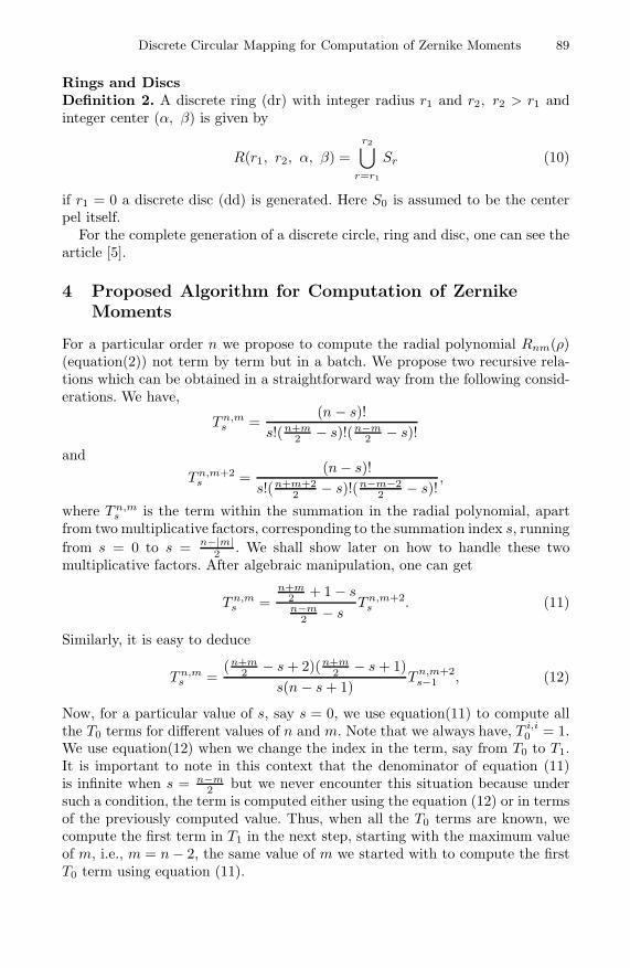
Discrete Circular Mapping for Computation of Zernike Moments 89
Rings and DiscsDefinition 2. A discrete ring (dr) with integer radius r1 and r2, r2 > r1 andinteger center (α, β) is given by
R(r1, r2, α, β) =r2⋃
r=r1
Sr (10)
if r1 = 0 a discrete disc (dd) is generated. Here S0 is assumed to be the centerpel itself.
For the complete generation of a discrete circle, ring and disc, one can see thearticle [5].
4 Proposed Algorithm for Computation of ZernikeMoments
For a particular order n we propose to compute the radial polynomial Rnm(ρ)(equation(2)) not term by term but in a batch. We propose two recursive rela-tions which can be obtained in a straightforward way from the following consid-erations. We have,
T n,ms =
(n − s)!s!(n+m
2 − s)!(n−m2 − s)!
and
T n,m+2s =
(n − s)!s!(n+m+2
2− s)!(n−m−2
2− s)!
,
where T n,ms is the term within the summation in the radial polynomial, apart
from two multiplicative factors, corresponding to the summation index s, runningfrom s = 0 to s = n−|m|
2. We shall show later on how to handle these two
multiplicative factors. After algebraic manipulation, one can get
T n,ms =
n+m2
+ 1 − sn−m
2 − sT n,m+2
s . (11)
Similarly, it is easy to deduce
T n,ms =
(n+m2
− s + 2)(n+m2
− s + 1)s(n − s + 1)
T n,m+2s−1 , (12)
Now, for a particular value of s, say s = 0, we use equation(11) to compute allthe T0 terms for different values of n and m. Note that we always have, T i,i
0 = 1.We use equation(12) when we change the index in the term, say from T0 to T1.It is important to note in this context that the denominator of equation (11)is infinite when s = n−m
2but we never encounter this situation because under
such a condition, the term is computed either using the equation (12) or in termsof the previously computed value. Thus, when all the T0 terms are known, wecompute the first term in T1 in the next step, starting with the maximum valueof m, i.e., m = n − 2, the same value of m we started with to compute the firstT0 term using equation (11).

90 R. Biswas and S. Biswas
4.1 Computational Analysis
For a P × P image,total number of multiplications can be shown to be
Nmult ≈ P/2(n2/4 + n + 1) + 64P 2 + NT + Sn + 14/8P 2 (13)
and the total number of additions as,
Nadd ≈ rmax + 53P 2 + 5[Sn/2 + 2(Sn/2−1+Sn/2−3 + · · · + S1)] + 6Sn + 7/8P 2.
(14)
where,NT = 8Sn/2 + 8(Sn/2−1 + Sn/2−3 + · · · + S1), (15)
4.2 Comparison
Below we present a comparison computational analysis of three other differentmethods, on an image of size P ×P and maximum order of Zernike moments M .Comparison shows that in the proposed method, number of multiplications dras-tically reduces and is minimum of all the cases. For additions, the number alsoreduces very significantly, except for the method described in [9] by Belkasim etal. Our method takes a slightly more number of additions than that of Belkasimet al. (approximately 1.38 times more) but it takes approximately 11.25 timesless number of multiplications than their method. This shows the effectiveness ofthe proposed method. It is obvious the Zernike moments are scale invariant. Ascomputations depend on the size (P) of the image it takes care the computationof scales.
Table 1. Comparison of multiplications and additions of different methods
References Number of additions Number of multiplications
[8] ≈ P 2M2/2 + 18PM3 ≈ 2M2 + P 2M2 + 1
4PM3
P=64, M=40 4,054,477 8,122,321
[9] ≈ M(P + 2)(P − 1) ≈ M2P2
2+ 2PM
P=64, M=40 166,320 3,281,920
[12] ≈ 38M2P + 2P 2M+ ≈ 1
2M2P + 2P 2M
P=64, M=40 112
M3P + 14M2P 2
2,562,198 397,358
Our method Equation (14) Equations (13), (15)P=64, M=40 230,289 291,164
Discrete Circular Mapping for Computation of Zernike Moments 91
5 Conclusion
Recently Zernike moments are gaining popularity in applications of patternrecognition, image analysis and image processing but direct computation offactorials in them is time consuming and discouraging. A faster algorithm istherefore necessary and its need is already felt to various research communities.We have presented an efficient algorithm that computes the Zernike momentsin a nice way. The comparison shows our algorithm is faster than the existingalgorithms. Also the mapping of pixels through discrete circles, maintains therotational invariance. The mapping is unique and leaves no holes or gaps on adisc.
References
1. Teague, M.R.: Image analysis via the general theory of moments. J. Opt. Soc.Am. 70(8), 920–930 (1980)
2. Teh, C., Chin, R.T.: On image analysis by the methods of moments. IEEE Trans.Pattern anal. Mach. Intell. 10(4), 496–513 (1988)
3. Khotanzad, A., Hong, Y.H.: Rotation invariant image recognition using featuresselected via a systematic method. Pattern Recognition 23(10), 1089–1101 (1990)
4. Liao, S.X., Pawlak, M.: On the accuracy of Zernike moments for image analysis.IEEE Trans. Pattern anal. Mach. Intell. 20, 1358–1364 (1998)
5. Bisaws, S.N., Chaudhuri, B.B.: On the generation of discrete circular objects andtheir properties. Comput. Vision, Graphics Image
6. Jiang, X.Y., Bunke, H.: Simple and fast computation of moments. Pattern Recog-nition 24(8), 801–806 (1991)
7. Li, B.C., Shen, J.: Fast computation of moment invariant. Pattern Recogni-tion 24(8), 807–813 (1991)
8. Mukundan, R., Ramakrishnan, K.R.: Fast computation of Legendre and Zernikemoments. Pattern Recognition 28(9), 1433–1442 (1995)
9. Belkasim, S.O., Ahmadi, M., Sridhar, M.: Efficient algorithm for fast computationof Zernike moments. J. Franklin Inst. Eng. Appl. Math. 333, 577–581 (1996)
10. Chan, F.H.Y., Lam, F.K.: An all adder systolic structure for fast computation ofmoments. J. VLSI Signal Process. 12, 159–175 (1996)
11. Shu, H.Z., Luo, L.M., Yu, W.X., Fu, Y.: A new fast method computing Legendremoments. Pattern Recognition 33(2), 341–348 (2000)
12. Gu, J., Su, H.Z., Toumoulin, C., Luo, L.M.: A novel algorithm for fast computationof Zernike moments. Pattern Recognition 35, 2905–2911 (2002)
13. Xin, Y., Pawlak, M., Liao, S.: Accurate computation of Zernike moments in polarcoordinates. IEEE Trans. on Image Processing 16(2), 581–587 (2007)
14. Wee, C.Y., Raveendran, P.: On the computational aspects of Zernike moments.Image and Vision Computing 25(6), 967–980 (2007)

Unsupervised Image Segmentation with
Adaptive Archive-Based EvolutionaryMultiobjective Clustering
Chin Wei Bong1 and Hong Yoong Lam2
1 School of Computer Science, Universiti Sains Malaysia2 Department of Cardiothoracic Surgery, Hospital Pulau Pinang
Penang, [email protected], [email protected]
Abstract. The aim of this paper is to propose and apply state-of-the-artmultiobjective scatter search for solving image segmentation problem.The algorithm incorporates the concepts of Pareto dominance, exter-nal archiving, diversification and intensification of solutions. The multi-objective optimization method is Archive-based Hybrid Scatter Search(AbYSS) for image segmentation. It utilized fuzzy clustering methodwith optimization of two fitness functions, viz., the global fuzzy compact-ness of the clusters and the fuzzy separation. We have tested the methodson two types of grey scale images, namely SAR (synthetic aperture radar)image and CT scan (Computer Tomography) image. We then comparedit with fuzzy c-means (FCM) and a popular evolutionary multiobjectiveevolutionary clustering named NSGA-II. The performance result for theproposed method is compatible with the existing methods.
Keywords: Multiobjective clustering, soft computing.
1 Introduction
Image segmentation process is defined as the extraction of the important objectsfrom an input image [1]. It partitions the pixels in the image into homogeneousregions, each of which corresponds to some particular information. There aremany approaches available for image segmentation including threshold methods[2], morphologic methods [3] and clustering algorithms. However, the segmenta-tion results from these methods are still not satisfactory.
Majority of existing clustering algorithms are based on only one internal evalu-ation function, which is a single-objective function that measures intrinsic prop-erties of a partitioning such as spatial separation between the clusters or thecompactness of the clusters. However, it is sometimes difficult to reflect thequality of partitioning reliably with only one internal evaluation function whichmay be violated for certain datasets [7]. In this paper, we use multiobjectiveoptimization (MOP) to overcome the defects of the single-objective clusteringalgorithms, such as FCM. Given that the objective functions (no less than two)for clustering are complementary, the simultaneous optimization of several of
S.O. Kuznetsov et al. (Eds.): PReMI 2011, LNCS 6744, pp. 92–97, 2011.c© Springer-Verlag Berlin Heidelberg 2011

Unsupervised Image Segmentation 93
those objectives may lead to high quality solutions and improve the robustnesstowards different data properties. MOCK proposed in [9] may be the first ap-plication of MOP in data clustering. However, only few applications have beenreported in image segmentation [10]. Among those applications, NSGA-II [8]was found to be the most popular method being used so far. It is difficult toapply current MOP clustering technology to image segmentation, owing to anextremely large amount of data need to be handled and thus the handling ofpopulation in an evolutionary algorithm (EA) is tedious.
Scatter search [4] is an EA in the sense that it incorporates the concept ofpopulation. As compared to other EA, it usually avoids using many randomcomponents, and it is based on using a small population, known as the referenceset, whose individuals are combined to construct new solutions which are gen-erated systematically. The reference set is initialized from an initial populationcomposed of diverse solutions, and it is updated with the solutions resultingfrom the local search improvement. Scatter search has been found to be success-ful in a wide variety of optimization problems [6], and until recently it had beenextended to deal with MOPs. Scatter search can act as a powerful local searchengine for tasks such as generating missing parts of a Pareto front because ofits flexibility and ease of use [11]. Therefore, this paper first proposes and ap-plies the state-of-the-art multiobjective scatter search for image segmentationusing Archive-based Hybrid Scatter Search (AbYSS). The framework incorpo-rates the concepts of Pareto dominance, external archiving, diversification andintensification of solution.
In the rest of this paper, we first present our proposal, followed by the exper-imental conducted to compare the proposed method with other standard imagesegmentation methods. Finally, we conclude the paper in the last section.
2 Multiobjective Clustering with AbYSS
The image segmentation problem is posed as clustering the pixels of the imagesin the intensity space. Here, a fuzzy clustering algorithm produces a membershipmatrix U(X) = [μkj ], k = 1, ..., K and j = 1, ..., n, where μkj denotes the mem-bership degree of pattern xj to cluster Ck. Here the individual are made up ofreal numbers which represent the coordinates of the cluster centers. If individualencodes the centers of Ki clusters in p dimensional space then its length li will bep×Ki. In the initial population, each string i encodes the centers of a some Ki
number of clusters, such that Ki = (rand()%K∗)+2, where rand() is a functionreturning a random integer, and K∗ is a soft estimate of the upper bound ofthe number of clusters [6]. Therefore, the number of clusters will vary from 2 toK∗ + 1. The Ki centers encoded in an individual of the initial population arerandomly selected distinct points from the input data set.
Two fitness functions, viz., the global fuzzy compactness J of the clustersand the fuzzy separation S are optimized simultaneously[5]. For computing theobjective functions, first the centers, V = v1, v2, ...vk encoded in a given indi-vidual are extracted. The fuzzy membership values μkj , i = 1, ..., K,k = 1, 2, ..., n

94 C.W. Bong and H.Y. Lam
are computed using μik =∑K
j=1D(vi,xk)D(vj ,xk)
−2/(m−1), 1 ≤ i ≤ K; 1 ≤ k ≤ n, where
D(vi, xk) denotes the distance between ith cluster center and kth data pointand m ∈ [1,∞] is the fuzzy exponent. Each cluster center vj = 1, 2, ..., K, isupdated using vi =
∑ nk=1 μm
ikxk∑ nk=1 μm
ik. The membership values are then recomputed.
The variation σi and fuzzy cardinality ni of the ith cluster,i = 1, 2, ..., K arecalculated as σi =
∑nk=1 μm
ikD(vi, xk), 1 ≤ i ≤ K and ni =∑n
k=1 μik, 1 ≤ i ≤ K.The global compactness of the solution represented by the chromosome is thencomputed as J =
∑Ki=1
σi
ni=
∑Ki=1
∑nk=1 μm
ikD(zi,xk)∑nk=1 μik
.The other fitness function fuzzy separation S is computed as follows: the
center vi of the ith cluster, is assumed to be the center of a fuzzy set . Hencethe membership degree of each vj to vi, j = i, is computed as
μij =∑K
l=1,l=jD(vi,vj)D(vj ,vl)
−2/(m−1), i = j.
Subsequently, the fuzzy separation is defined as S=∑K
i=1
∑Ki=1,j =i μm
ij D(vi, vj).In order to obtain compact clusters, the measure J should be minimized. On thecontrary, to get well separated clusters, the fuzzy separation S should be maxi-mized. As in this article the multiobjective problem is posed as minimization ofboth the objectives, hence the objective is to minimize J and 1
Ssimultaneously.
AbYSS is based on the scatter search template adopted from [4]. The tem-plate defines six methods, as depicted in Figure 1, are described below:
1) Diversification Generation Procedure: The procedure is the same as that pro-posed in [4]. The goal is to generate an initial set P of diverse solutions. Thisis a simple method based on dividing the range of each variable into a numberof subranges of equal size; then, the value for each variable of every solution isgenerated.2) Improvement procedure: This procedure is to use a local search algorithm(a simplex method) to improve new solutions obtained from the diversificationgeneration and solution combination methods. The improvement method takesan individual as a parameter, which is repeatedly mutated with the aim of ob-taining a better individual. The term ”better” is defined here in a similar wayto the constrained-dominance approach used in NSGA-II [8].3) Reference Set Update procedure: The reference set is a collection of bothhigh-quality and diverse solutions that are used to generate new individuals.The set itself is composed of two subsets, RefSet1 and RefSet2, of size p andq, respectively. The first subset contains the best quality solutions in P , whilethe second subset should be filled with solutions promoting diversity.4) Subset Generation procedure: This procedure generates subsets of individu-als, which will be used to create new solutions with the solution combinationmethod. The strategy used considers all pairwise combinations of solutions inthe reference set [7]. Furthermore, this method should avoid producing repeatedsubsets of individuals, i.e., subsets previously generated.

Unsupervised Image Segmentation 95
Fig. 1. Template for the six methods in the proposed framework
5) Solution Combination procedure: This procedure is to find linear combinationsof reference solutions. The use of a simulated binary crossover operator (SBX)makes AbYSS more robust [6].6) Adaptive Memory Procedure: The aim of External Archive is to store a recordof the non-dominated individuals found during the search in order to keep thoseindividuals producing a well distributed Pareto front. This archive is empty atthe beginning of the method. We will continuously update it whenever a newindividual or solution is not dominated by the RefSet1. Besides, we use thefollowing rules to reduce the computational requirements: (a) New solution yobtained from x should be used to update External Archive only if it is notdominated by x. (b) New potentially Pareto-optimal solutions could be added toExternal Archive only if they differ enough from all solutions already containedin this set. We propose to use a threshold defining the minimum Euclideandistance in the space of normalized objectives between solutions in ExternalArchive. A new potentially Pareto optimal solution is neglected if it is closer toat least one solution in External Archive than the threshold. We have observedexperimentally that the solutions added to External Archive in early iterationshave a good chance to be removed from this set in further iterations. In otherwords the time spent on updating External Archive in early iterations is likelyto be lost. Thus, it is possible to neglect updating External Archive in a numberof starting iterations.
Initially, the diversification generation method is invoked to generate initialsolutions, and each one is passed to the improvement method and the result is theinitial set P . Then, a fix number of iterations are performed. At each iteration,the reference set is built, the subset generation method is invoked, and themain loop of the scatter search algorithm is executed until the subset generationmethod stops producing new subsets of solutions. Then, there is a restart phase,which consists of three steps. First, the individuals RefSet1 in are inserted into

96 C.W. Bong and H.Y. Lam
P ; second, the best individuals n from the external archive, according to thecrowding distance, are also moved to P ; and, third, the diversification generationand improvement methods are used to produce new solutions for filling up theset P . The idea of moving n individuals from the archive to the initial set is topromote the intensification capabilities of the search towards the Pareto frontalready found. The intensification degree can vary depending on the number ofchosen individuals. The best single solution is then selected based on the methodintroduced by MetaClustering algorithm (MCLA)[5].
3 Experimental Study
We have compared our algorithm with standard FCM and a popular evolutionarymultobjective clustering, NSGA-II. For NSGA-II, we executed 100 generationswith fixed population size 50. The crossover and mutation probabilities are fixedas 0.8 and 0.01, respectively. FCM is executed for a maximum of 100 iterations,with m, the fuzzy exponent, equal to 2.0. First, the experiment was done for a 3-class SAR images obtained from http://www.sandia.gov/radar/imageryku.html.The image is a Ku-band SAR image with one meter spatial resolution in the areaof Rio Grande River near Albuquerque, New Mexico, USA. This image consistsof three types of land cover, namely, the river, the vegetation and the crop.Then, the experiment was extended to real CT scan image for Lung obtainedfrom Penang Hospital, Malaysia. The results of the algorithms are compared
with two cluster validity functions: partition coefficient, Vpc(U) =∑ n
j=1∑ c
i=1 μ2ij
nand partition entropy value, Vpe(U ) = 1
n
∑nj=1
∑ci=1 μij log μij [7]. The cluster-
ing result is better with a higher Vpc(U) value and a lower Vpe(U) value. Table 1shows the performance comparison of FCM, NSGA-II and the proposed methodin terms of cluster validity functions with both index. The values of Vpc(U) arehigher in the proposed method than the FCM and NSGA-II methods. Mean-while, the values of Vpe(U) are lower in the proposed method than the FCMand NSGA-II methods. This result indicates that the proposed method is out-performed than other two methods. Fig. 2 shows the example of images andtheir segmented results. For SAR image, FCM and the proposed method arebetter than NSGA-II in terms of the regional consistency of the water and thebuildings region. However, all the three algorithms cannot achieve the visuallycorrect segmentation in the right top region, i.e. FCM, and the proposed methodmisclassifies a big area of land region as the water. Comparatively, the proposedmethod performs best in this area where the misclassification is not so seriousas FCM and NSGA-II.
Table 1. Result of partition coefficient and partition entropy for the two types ofimages with different methods
Methods Index FCM NSGA-II Proposed Index FCM NSGA-II Proposed
SAR IMAGE Vpe 0.14230 0.14025 0.11227 Vpc 0.91031 0.91106 0.92180
CT Scan IMAGE Vpe 0.06910 0.05150 0.0403 Vpc 0.93113 0.94170 0.95943
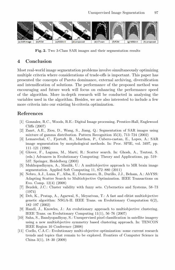
Unsupervised Image Segmentation 97
Fig. 2. Two 3-Class SAR images and their segmentation results
4 Conclusion
Most real-world image segmentation problems involve simultaneously optimizingmultiple criteria where considerations of trade-offs is important. This paper haspresented the concepts of Pareto dominance, external archiving, diversificationand intensification of solutions. The performance of the proposed method wasencouraging and future work will focus on enhancing the performance speedof the algorithm. More in-depth research will be conducted in analysing thevariables used in the algorithm. Besides, we are also interested to include a fewmore criteria into our existing bi-criteria optimization.
References
[1] Gonzalez, R.C., Woods, R.E.: Digital Image processing. Prentice-Hall, EnglewoodCliffs (2007)
[2] Zaart, A.E., Ziou, D., Wang, S., Jiang, Q.: Segmentation of SAR images usingmixture of gamma distribution. Pattern Recognition 35(3), 713–724 (2002)
[3] Lemarechal, C., Fjortoft, R., Marthon, P., Cubero-castan, E., Lopes, A.: SARimage segmentation by morphological methods. In: Proc. SPIE, vol. 3497, pp.111–121 (1998)
[4] Glover, F., Laguna, M., Martı, R.: Scatter search. In: Ghosh, A., Tsutsui, S.(eds.) Advances in Evolutionary Computing: Theory and Applications, pp. 519–537. Springer, Heidelberg (2003)
[5] Mukhopadhyaya, A., Maulik, U.: A multiobjective approach to MR brain imagesegmentation. Applied Soft Computing 11, 872–880 (2011)
[6] Nebro, A.J., Luna, F., Alba, E., Dorronsoro, B., Durillo, J.J., Beham, A.: AbYSS:Adapting Scatter Search to Multiobjective Optimization. IEEE Transactions onEvo. Comp. 12(4) (2008)
[7] Bezdek, J.C.: Cluster validity with fuzzy sets. Cybernetics and Systems, 58–73(1974)
[8] Deb, K., Pratap, A., Agarwal, S., Meyarivan, T.: A fast and elitist multiobjectivegenetic algorithm: NSGA-II. IEEE Trans. on Evolutionary Computation 6(2),182–197 (2002)
[9] Handl, J., Knowles, J.: An evolutionary approach to multiobjective clustering.IEEE Trans. on Evolutionary Computing 11(1), 56–76 (2007)
[10] Saha, S., Bandyopadhyay, S.: Unsupervised pixel classification in satellite imageryusing a new multiobjective symmetry based clustering approach. In: TENCONIEEE Region 10 Conference (2008)
[11] Coello, C.A.C.: Evolutionary multi-objective optimization: some current researchtrends and topics that remain to be explored. Frontiers of Computer Science inChina 3(1), 18–30 (2009)
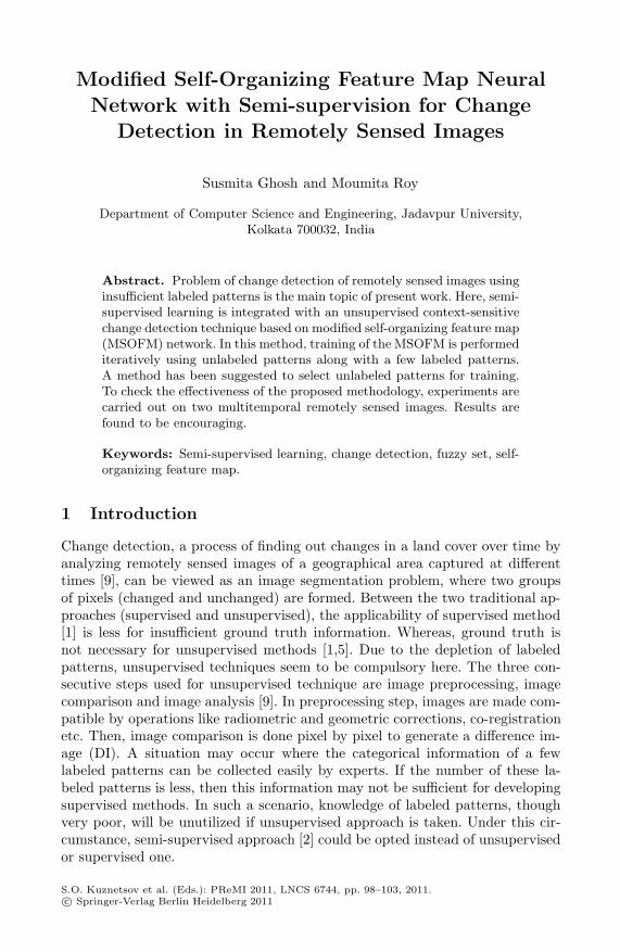
Modified Self-Organizing Feature Map Neural
Network with Semi-supervision for ChangeDetection in Remotely Sensed Images
Susmita Ghosh and Moumita Roy
Department of Computer Science and Engineering, Jadavpur University,Kolkata 700032, India
Abstract. Problem of change detection of remotely sensed images usinginsufficient labeled patterns is the main topic of present work. Here, semi-supervised learning is integrated with an unsupervised context-sensitivechange detection technique based on modified self-organizing feature map(MSOFM) network. In this method, training of the MSOFM is performediteratively using unlabeled patterns along with a few labeled patterns.A method has been suggested to select unlabeled patterns for training.To check the effectiveness of the proposed methodology, experiments arecarried out on two multitemporal remotely sensed images. Results arefound to be encouraging.
Keywords: Semi-supervised learning, change detection, fuzzy set, self-organizing feature map.
1 Introduction
Change detection, a process of finding out changes in a land cover over time byanalyzing remotely sensed images of a geographical area captured at differenttimes [9], can be viewed as an image segmentation problem, where two groupsof pixels (changed and unchanged) are formed. Between the two traditional ap-proaches (supervised and unsupervised), the applicability of supervised method[1] is less for insufficient ground truth information. Whereas, ground truth isnot necessary for unsupervised methods [1,5]. Due to the depletion of labeledpatterns, unsupervised techniques seem to be compulsory here. The three con-secutive steps used for unsupervised technique are image preprocessing, imagecomparison and image analysis [9]. In preprocessing step, images are made com-patible by operations like radiometric and geometric corrections, co-registrationetc. Then, image comparison is done pixel by pixel to generate a difference im-age (DI). A situation may occur where the categorical information of a fewlabeled patterns can be collected easily by experts. If the number of these la-beled patterns is less, then this information may not be sufficient for developingsupervised methods. In such a scenario, knowledge of labeled patterns, thoughvery poor, will be unutilized if unsupervised approach is taken. Under this cir-cumstance, semi-supervised approach [2] could be opted instead of unsupervisedor supervised one.
S.O. Kuznetsov et al. (Eds.): PReMI 2011, LNCS 6744, pp. 98–103, 2011.c© Springer-Verlag Berlin Heidelberg 2011

Semi-supervised Change Detection Using MSOFM 99
In the present work, a neural network based semi-supervised change detectionmethod is proposed. Here, the idea of semi-supervised learning [2] is incorpo-rated into the existing unsupervised change detection technique based on theMSOFM network [6]. This work is inspired from a work on change detectionusing semi-supervised multilayer perceptron (MLP) [8]. The MSOFM network[4,6] has two layers: input and output. For each feature of the input pattern,there is a neuron in the input layer. The output layer is two dimensional andthere is a representative neuron for each pixel position of DI. In the presentwork, change vector analysis (CVA) technique [1,9] is used for generating DI.The input pattern for a particular pixel position is generated using gray value ofthe said pixel as well as those of its neighborhood pixels for considering (spatial)contextual information from neighbors. In the present work 2nd order neighbor-hood is used. A mapping algorithm [4,6] is used to normalize the feature valuesof the input pattern in [0, 1]. Each neuron in the output layer is connected toall the neurons in the input layer. The connection weights of the representativeneuron of the labeled pixel position are initialized with the normalized featurevalues of the corresponding labeled pattern; whereas the weight vector for othersis initialized randomly between [0, 1]. Iterative learning of the MSOFM networkis performed by the labeled patterns along with the selected unlabeled patternsuntil a given convergence criterion is satisfied.
2 Kohonen’s Self-Organizing Feature Map
In the proposed algorithm, we have used the same MSOFM network as usedin [4,6]. The MSOFM network is motivated from the Kohonen’s self-organizingfeature maps (SOFM) [7] and has similar network structure as that of the SOFM.SOFM is learned iteratively and generates topological map of input patternsgradually. The input pattern is represented by −→
X and −→Wj denotes the synaptic
weight vector of jth output neuron (where j = 1, 2, ..., z and z be the number ofneurons in the output layer). The winner neuron j in the output layer is selectedas the best-matched neuron for the given input pattern where the similaritymeasure (−→Wj · −→X ) is maximum. Let, h(itr) be the topological neighborhoodfunction at iteration itr that shrinks after each iteration. The weight updatingof winning neuron is done as,
−→W (itr + 1) = −→
W (itr) + h(itr)η(itr)(−→X −−→W (itr)), (1)
where, η(itr) denotes the learning rate in iteration itr and decreases with increaseof itr.
3 The Proposed Algorithm
In the present technique, labeled patterns from both the classes are pickedup randomly from the ground truth. Let, the y-dimensional input pattern of(m, n)th pixel position of DI is denoted by −−→
Xmn = [xmn,1, xmn,2, ..., xmn,y]. The

100 S. Ghosh and M. Roy
y-dimensional weight vector between (m, n)th neuron in the output layer and allthe neurons of the input layer is represented by −−−→
Wmn = [wmn,1, wmn,2, ..., wmn,y].During training, input patterns −−→Xmn are passed to the network one by one. Eachtime, the dot product d(m, n) between −−→
Xmn and −−−→Wmn is calculated as,
d(m, n) = −−→Xmn · −−−→Wmn =
y∑
k=1
xmn,k · wmn,k. (2)
At the beginning of the training phase, the connection weights of the MSOFMnetwork are updated in the following manner using the labeled patterns only.If the class label of the (m, n)th pixel position is known, then the weight vector−−→Wij for all neighboring neurons (defined by hmn(.)) of (m, n)th output neuronis updated using equation (1), iff (i, j)th input pattern is unlabeled. For thelabeled patterns, the weight vector is not updated during the entire learning pro-cess. Learning using labeled patterns is continued iteratively until convergence.To check convergence, O(itr) is calculated at each iteration using,
O(itr) =∑
d(m,n)≥t
d(m, n), (3)
where, t is a predefined threshold value [6]. The weight updating is preformeduntil (O(itr)−O(itr−1)) < δ, where δ is a small positive quantity. The value oft varies within [0, 1]. The components of the weight vector −−−→Wmn are normalizedin a way so that the dot product d(m, n) lies between [0, 1]. After each epoch, thelearning rate η(itr) and the size of the topological neighborhood h(itr) decrease.
After each training step, the soft class labels of unlabeled patterns are calcu-lated by presenting them to the network. Let us consider that there exists twofuzzy sets: one for the changed class and the other for unchanged one. For each(i, j)th unlabeled pattern, d(i, j) is computed by equation (2); if, d(i, j) ≥ t, then(i, j)th pattern is more likely to belong to changed class than unchanged one; elsein unchanged class. Let, μ(i, j) = [μ1(i, j), μ2(i, j)] be the membership value of(i, j)th unlabeled pattern, where μ1(i, j) and μ2(i, j) are the membership valuesin unchanged class and changed class, respectively. The values can be calculatedas,
[μ1(i, j), μ2(i, j)] =
⎧⎪⎪⎪⎪⎨
⎪⎪⎪⎪⎩
[min(d(i, j), 1 − d(i, j)),max(d(i, j), 1 − d(i, j))] if d(i, j) ≥ t
[max(d(i, j), 1 − d(i, j)),min(d(i, j), 1 − d(i, j))] Otherwise.
(4)
After that, the target value of the unlabeled pattern is updated by K-nearestneighbor technique as it was used in [8]. To search for K-nearest neighbors,instead of considering all the patterns, we consider only those which lie within awindow around that unlabeled pattern. Let, M be the set of K-nearest neighborsof (i, j)th unlabeled pattern. Now, target value t(i, j) = [t1(i, j), t2(i, j)] of (i, j)th
unlabeled pattern is estimated as,
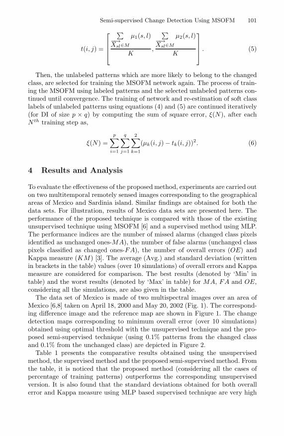
Semi-supervised Change Detection Using MSOFM 101
t(i, j) =
⎡
⎢⎢⎣
∑−→Xsl∈M
μ1(s, l)
K,
∑−→Xsl∈M
μ2(s, l)
K
⎤
⎥⎥⎦ . (5)
Then, the unlabeled patterns which are more likely to belong to the changedclass, are selected for training the MSOFM network again. The process of train-ing the MSOFM using labeled patterns and the selected unlabeled patterns con-tinued until convergence. The training of network and re-estimation of soft classlabels of unlabeled patterns using equations (4) and (5) are continued iteratively(for DI of size p × q) by computing the sum of square error, ξ(N), after eachN th training step as,
ξ(N) =p∑
i=1
q∑
j=1
2∑
k=1
(μk(i, j) − tk(i, j))2. (6)
4 Results and Analysis
To evaluate the effectiveness of the proposed method, experiments are carried outon two multitemporal remotely sensed images corresponding to the geographicalareas of Mexico and Sardinia island. Similar findings are obtained for both thedata sets. For illustration, results of Mexico data sets are presented here. Theperformance of the proposed technique is compared with those of the existingunsupervised technique using MSOFM [6] and a supervised method using MLP.The performance indices are the number of missed alarms (changed class pixelsidentified as unchanged ones-MA), the number of false alarms (unchanged classpixels classified as changed ones-FA), the number of overall errors (OE) andKappa measure (KM) [3]. The average (Avg.) and standard deviation (writtenin brackets in the table) values (over 10 simulations) of overall errors and Kappameasure are considered for comparison. The best results (denoted by ‘Min’ intable) and the worst results (denoted by ‘Max’ in table) for MA, FA and OE,considering all the simulations, are also given in the table.
The data set of Mexico is made of two multispectral images over an area ofMexico [6,8] taken on April 18, 2000 and May 20, 2002 (Fig. 1). The correspond-ing difference image and the reference map are shown in Figure 1. The changedetection maps corresponding to minimum overall error (over 10 simulations)obtained using optimal threshold with the unsupervised technique and the pro-posed semi-supervised technique (using 0.1% patterns from the changed classand 0.1% from the unchanged class) are depicted in Figure 2.
Table 1 presents the comparative results obtained using the unsupervisedmethod, the supervised method and the proposed semi-supervised method. Fromthe table, it is noticed that the proposed method (considering all the cases ofpercentage of training patterns) outperforms the corresponding unsupervisedversion. It is also found that the standard deviations obtained for both overallerror and Kappa measure using MLP based supervised technique are very high
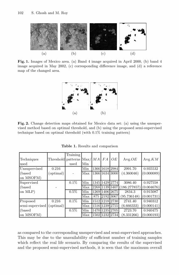
102 S. Ghosh and M. Roy
(a) (b) (c) (d)
Fig. 1. Images of Mexico area. (a) Band 4 image acquired in April 2000, (b) band 4image acquired in May 2002, (c) corresponding difference image, and (d) a referencemap of the changed area.
(a) (b)
Fig. 2. Change detection maps obtained for Mexico data set: (a) using the unsuper-vised method based on optimal threshold, and (b) using the proposed semi-supervisedtechnique based on optimal threshold (with 0.1% training pattern)
Table 1. Results and comparison
Techniquesused
ThresholdTrainingpatterns
usedMax/Min
MA FA OE Avg.OE Avg.KM
Unsupervised 0.216 Min 1366 1618 2984 2991.70 0.935532(basedon MSOFM)
(optimal) - Max 1366 1634 3000 (4.360046) (0.000089)
Supervised 0.1% Min 1345 1429 2774 3086.40 0.927558(based - Max 2268 1139 3407 (186.277857) (0.004676)on MLP) 0.5% Min 1269 1406 2675 2834.3 0.915087
Max 875 2192 3067 (95.736148) (0.001731)
Proposed 0.216 0.1% Min 1512 1218 2730 2741.40 0.940312semi-supervised (optimal) Max 1516 1239 2755 (6.666333) (0.000141)(based 0.5% Min 1470 1235 2705 2723.70 0.940475on MSOFM) Max 1502 1232 2734 (8.331266) (0.000193)
as compared to the corresponding unsupervised and semi-supervised approaches.This may be due to the unavailability of sufficient number of training sampleswhich reflect the real life scenario. By comparing the results of the supervisedand the proposed semi-supervised methods, it is seen that the maximum overall

Semi-supervised Change Detection Using MSOFM 103
error (denoted by ‘Max’) obtained by the semi-supervised approach is less thanthat of the corresponding supervised method. In short, the results show that theproposed semi-supervised version has an edge over the unsupervised as well asthe supervised techniques when a few labeled patterns are available.
5 Conclusion
In this paper, an attempt has been made to improve the performance of changedetection of remotely sensed images under the scarcity of sufficient number oflabeled patterns by exploring the self-organizing capacity of Kohonen’s networkintegrated with semi-supervision. From the results, it has been found that theproposed algorithm is better suited for change detection where a small amountof labeled patterns is available.
Acknowledgments. The authors like to thank the Department of Science andTechnology (DST), Government of India and University of Trento, Italy, thesponsors of the ITPAR program and Prof. L. Bruzzone, the Italian collaboratorof this project, for providing the data.
References
1. Canty, M.J.: Image Analysis, Classification and Change Detection in Remote Sens-ing. CRC Press, Taylor & Francis (2006)
2. Chapelle, O., Scholkopf, B., Zien, A.: Semi-supervised Learning. MIT Press, Cam-bridge (2006)
3. Congalton, R.G., Green, K.: Assessing the Accuracy of Remotely Sensed Data:Principles and Practices, 2nd edn. CRC Press, Taylor & Francis Group (2009)
4. Ghosh, A., Pal, S.K.: Neural network, self-organization and object extraction. Pat-tern Recognition Letters 13, 387–397 (1992)
5. Ghosh, A., Mishra, N.S., Ghosh, S.: Fuzzy clustering algorithms for unsupervisedchange detection in remote sensing images. Information Sciences 181(4), 699–715(2011)
6. Ghosh, S., Patra, S., Ghosh, A.: An unsupervised context-sensitive change detectiontechnique based on modified self-organizing feature map neural network. Interna-tional Journal of Approximate Reasoning 50(1), 37–50 (2009)
7. Kohonen, T.: Self-Organizing Maps, 2nd edn. Springer, Berlin (1997)8. Patra, S., Ghosh, S., Ghosh, A.: Change detection of remote sensing images
with semi-supervised multilayer perceptron. Fundamenta Informaticae 84, 429–442(2008)
9. Singh, A.: Digital change detection techniques using remotely sensed data. Interna-tional Journal of Remote Sensing 10(6), 989–1003 (1989)

Image Retargeting through Constrained Growth
of Important Rectangular Partitions
Rajarshi Pal1, Jayanta Mukhopadhyay2, and Pabitra Mitra2
1 Center for Soft Computing Research, Indian Statistical Institute, Kolkata, India2 Department of Computer Science and Engineering, Indian Institute of Technology,
Kharagpur, India
Abstract. The challenge of displaying an image in a much smaller tar-get area is to maintain recognizability of its contents. A novel rectangularpartitioning based retargeting scheme is proposed in this paper to ad-dress this issue. Constrained growth of rectangular partitions containingimportant objects is major characteristic of this scheme. Subjective eval-uation by a group of volunteers establishes usefulness of this scheme.
Keywords: Image retargeting.
1 Introduction
Resizing an image, even of moderate size, to display it on a small gadget (suchas, cell-phones) reduces recognizability of its contents. Content-aware process-ing addresses this issue by differentiating image contents on the basis of theirimportance. Image cropping [1,2,3] and fisheye-view warping [4] are effective forimages with single important object. But they are not that much effective whenimportant contents are sparsely distributed within the image. Unimportant con-tents still occupy a major portion of the display in such case. Rapid Serial VisualPresentation (RSVP) [5] displays important portions of the image one-by-one.
On the other hand, seam carving (originally proposed by [6]) and optimizedscale-and-stretch warping [7] are effective irrespective of spatial distribution ofimportant contents within the image. Seam carving fits an image to the targetspace by iteratively removing seams that pass through less important contentsof the image. Removing excessive number of seams to fit the image in smalltarget space often induces distortion. Later on, controlled seam carving [8,9]strategies have been proposed to check such distortion. Optimized scale-and-stretch warping [7] iteratively computes local scaling factors for each local region.
This paper introduces another novel scheme that also can operate irrespectiveof spatial distribution of important contents. Relative enlargement of importantcontents is estimated here by considering their size and spatial positioning only.A simplistic rectangular partitioning of image space based on the importance ofeach individual content and similar partitioning of the target space add noveltyto the proposed scheme. Unlike some previous literature on image retargeting,this paper does not focus on deriving importance of individual image content.Rather it focuses only on how important contents can be enlarged.
S.O. Kuznetsov et al. (Eds.): PReMI 2011, LNCS 6744, pp. 104–109, 2011.c© Springer-Verlag Berlin Heidelberg 2011

Image Retargeting through Constrained Growth 105
The organization of the paper is as follows: A brief discussion on extractingrectangular regions of importance is presented in section 2. In section 3, theretargeting scheme is described where important rectangles are disproportion-ately enlarged. Section 4 discusses about subjective control over the relative sizechange to obtain distortion free result. Results along with subjective evaluationare presented in section 5. Finally, conclusions are drawn in section 6.
2 Region of Importance Extraction
Visual attention models which compute saliency based on low-level image fea-tures are commonly used in deriving importance of image contents. The saliencymodel in [10] is used here for our experiments as recent experiments have estab-lished its superiority as compared to others (for e.g., the model in [11]). Facedetectors [12,13] can also be combined with saliency models to incorporate somesemantic knowledge in importance computation. Though face detection moduleis not considered in our current study.
Once the importance map is obtained, important objects are extracted asfollows. A line parallel to X -axis passing through the center point of the impor-tance map partitions it in two portions: L and R. Again, a line parallel to Y -axispassing through this center point partitions the importance map in two portions:U and B. Let ML, MR, MU and MB be the maximum importance values in L,R, U and B, respectively. A threshold Ts is fixed at p% of the lowest of thesefour importance values.
Ts = p/100 ∗ min (ML, MR, MU , MB) (1)
Then the importance map is binarized using the threshold Ts to get pixelswith high importance. Each set of connected important pixels form one impor-tant object. For ease of computation, we do away with the irregular shapes ofimportant objects using a minimum rectangle ri for each important object i. Thesaliency map along with important rectangles identified for an image is shownin Figure 1.
Fig. 1. A sample input image (left) and important rectangles superimposed on theimportance map of the image (right)

106 R. Pal, J. Mukhopadhyay, and P. Mitra
3 Proposed Retargeting Scheme
The retargeting scheme, proposed in this section, uses the important rectanglesidentified in previous section to generate the retargeted image.
3.1 Initial Position of Important Rectangles in Target Space
Edges of the important rectangles are parallel to the horizontal and verticalaxis. Such a rectangle ri can be specified by its top-left and bottom-right cornerpoints. Let, (ci, di) and (fi, gi) are these points for ri in the original image.Scaled down versions of the important rectangles are positioned in the targetspace (i.e., smaller display). Their positions in the target space are indicated byend points of main diagonal (ct, dt) and (ft, gt). These points are estimated asfollows:
(ct, dt) = (⌈
ci ht
hi
⌉,
⌈di wt
wi
⌉) (2)
(ft, gt) = (⌈
fi ht
hi
⌉,
⌈gi wt
wi
⌉) (3)
where hi and wi are height and width of the original image, respectively. ht
and wt denote height and width of the target space, respectively. · returns thesmallest integer greater than or equal to its input argument.
3.2 Growing Important Rectangles in Target Space
Important rectangles are allowed to grow within the target space. But few basicconstraints are also maintained to prevent arbitrary growth of these rectangles.These constraints are:
1. Aspect ratio of each important rectangle is preserved.2. All important rectangles are enlarged equally.3. Rectangles do not cross the boundary of target space while being grown.4. Relative ordering in position of the horizontal and vertical edges of these
rectangles is preserved.
To ensure condition 1, height and width of a rectangle are multiplied withequal resizing gain factor λ. Condition 2 is preserved by enlarging all the rect-angles with equal value for λ. It is also checked whether boundary of a rectanglecrosses the boundary of the target space (condition 3). If it crosses the tar-get space boundary, it is translated back into target space. Across any direction(vertical or horizontal), relative ordering of horizontal and vertical edges of theserectangles is maintained (condition 4). To maintain relative ordering of horizon-tal edges, rank correlation coefficient of x coordinates of the corner points beforeand after enlargement is checked. If there is no change in ordering, the value ofthe coefficient will be 1. Similar checking with y coordinates preserves relativeordering of vertical edges. Condition 4 also ensures that there is no overlapping
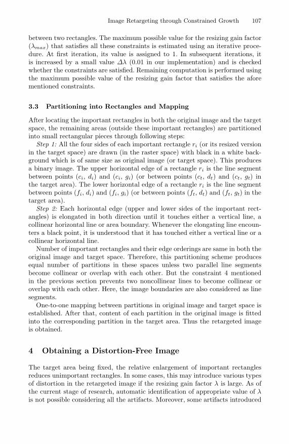
Image Retargeting through Constrained Growth 107
between two rectangles. The maximum possible value for the resizing gain factor(λmax) that satisfies all these constraints is estimated using an iterative proce-dure. At first iteration, its value is assigned to 1. In subsequent iterations, itis increased by a small value Δλ (0.01 in our implementation) and is checkedwhether the constraints are satisfied. Remaining computation is performed usingthe maximum possible value of the resizing gain factor that satisfies the aforementioned constraints.
3.3 Partitioning into Rectangles and Mapping
After locating the important rectangles in both the original image and the targetspace, the remaining areas (outside these important rectangles) are partitionedinto small rectangular pieces through following steps:
Step 1: All the four sides of each important rectangle ri (or its resized versionin the target space) are drawn (in the raster space) with black in a white back-ground which is of same size as original image (or target space). This producesa binary image. The upper horizontal edge of a rectangle ri is the line segmentbetween points (ci, di) and (ci, gi) (or between points (ct, dt) and (ct, gt) inthe target area). The lower horizontal edge of a rectangle ri is the line segmentbetween points (fi, di) and (fi, gi) (or between points (ft, dt) and (ft, gt) in thetarget area).
Step 2: Each horizontal edge (upper and lower sides of the important rect-angles) is elongated in both direction until it touches either a vertical line, acollinear horizontal line or area boundary. Whenever the elongating line encoun-ters a black point, it is understood that it has touched either a vertical line or acollinear horizontal line.
Number of important rectangles and their edge orderings are same in both theoriginal image and target space. Therefore, this partitioning scheme producesequal number of partitions in these spaces unless two parallel line segmentsbecome collinear or overlap with each other. But the constraint 4 mentionedin the previous section prevents two noncollinear lines to become collinear oroverlap with each other. Here, the image boundaries are also considered as linesegments.
One-to-one mapping between partitions in original image and target space isestablished. After that, content of each partition in the original image is fittedinto the corresponding partition in the target area. Thus the retargeted imageis obtained.
4 Obtaining a Distortion-Free Image
The target area being fixed, the relative enlargement of important rectanglesreduces unimportant rectangles. In some cases, this may introduce various typesof distortion in the retargeted image if the resizing gain factor λ is large. As ofthe current stage of research, automatic identification of appropriate value of λis not possible considering all the artifacts. Moreover, some artifacts introduced

108 R. Pal, J. Mukhopadhyay, and P. Mitra
due to relative size change of important and unimportant objects may be ofsubjective nature. Therefore, a possible implementation of the proposed schemeis as follows: It presents the viewer with a retargeted image with λ = λmax. If theviewer is not satisfied with the quality of the result, she is allowed to graduallydecrease the value of λ until the desired quality is obtained.
5 Results and Discussions
The proposed scheme is tested using 100 images. Results for these were generatedusing a λ value that suits the subjective quality according to our observation.These results are compared against those from cropping [1] and controlled seamcarving [8]. The results obtained for some of the images are shown in Figure 2.To test the effectiveness of various retargeting strategies, it is necessary to pre-pare the outcomes of the comparing schemes using the same importance map.Therefore, the saliency [10] based importance map is used for all three concernedmethods. The results of these retargeting schemes are presented in Figure 2. Itcan be observed from Figure 2 that enlargement of the important objects is muchin the proposed scheme as compared to other schemes at the presence of multipleimportant objects. Performance of the proposed scheme is also comparable toother schemes for images with single important object.
Fig. 2. Columns from left to right: down sampled version of the original image, out-put of the proposed scheme, image cropping [1] and seam curving base method [8],respectively
Evaluation of retargeting is essentially of subjective nature. Hence, it is re-sorted to manual judgments for evaluation. All the results were presented toforty-one volunteers. They were asked to evaluate each result of each schemeas either good (score 2), average (score 1) or poor (score 0). For each scheme,scores of 100 images are summed up to find a score for that scheme. Meanscore is computed for each scheme over scores given by all volunteers. Averagescore per image (and per volunteer) of the proposed rectangle partitioning basedscheme is 1.39, whereas those for the cropping and the controlled seam curvingbased scheme are 0.99 and 1.09, respectively. Therefore, subjective evaluationdemonstrates the usefulness of the proposed scheme over cropping and seamcarving.

Image Retargeting through Constrained Growth 109
6 Conclusion
Enlarging important contents of the image through a rectangular partition basedscheme restores their recognizability. All important objects are enhanced uni-formly and their aspect ratios are kept unchanged. Relative ordering of theirplacement in the target area is also kept same as that in the original image.Ability to perform in the presence of multiple sparsely distributed importantobjects is another notable point for the proposed scheme.
References
1. Suh, B., Ling, H., Bederson, B.B., Jacobs, D.W.: Automatic thumbnail croppingand its effectiveness. In: Proc. of 16th Annual Symposium on User Interface Soft-ware and Technology, November 2003, pp. 95–104 (2003)
2. Luo, J.: Subject content-based intelligent cropping for digital photos. In: Proc. ofIEEE International Conference on Multimedia and Expo, July 2007, pp. 2218–2221(2007)
3. Ciocca, G., Cusano, C., Gasparini, F., Schettini, R.: Self-adaptive image crop-ping for small displays. IEEE Transactions on Consumer Electronics 53, 1622–1627(2007)
4. Liu, F., Gleicher, M.: Automatic image retargeting with fisheye-view warping. In:Proc. of 18th Annual ACM Symposium on User Interface Software and Technology,October 2005, pp. 153–162 (2005)
5. Fan, X., Xie, X., Ma, W.Y., Zhang, H.J., Zhou, H.Q.: Visual attention based imagebrowsing on mobile devices. In: Proc. of International Conference on Multimediaand Expo (July 2003)
6. Avidan, S., Shamir, A.: Seam carving for content-aware image resizing. ACMTransactions on Graphics 26 (July 2007)
7. Wang, Y.S., Tai, C.L., Sorkine, O., Lee, T.Y.: Optimized scale-and-stretch forimage resizing. ACM Transactions on Graphics 27 (December 2008)
8. Hwang, D.S., Chien, S.Y.: Content-aware image resizing using perceptual seamcarving with human attention model. In: Proc. of IEEE International Conferenceon Multimedia and Expo, June 2008, pp. 1029–1032 (2008)
9. Utsugi, K., Shibahara, T., Koike, T., Naemura, T.: Proportional constraint forseam carving. In: Proc. of International Conference on Computer Graphics andInteractive Techniques (August 2009)
10. Pal, R., Mukherjee, A., Mitra, P., Mukherjee, J.: Modelling visual saliency usingdegree centrality. IET Computer Vision 4(3), 218–229 (2010)
11. Itti, L., Koch, C., Niebur, E.: A model of saliency-based visual attention forrapid scene analysis. IEEE Transactions on Pattern Analysis and Machine Intelli-gence 20(11), 1254–1259 (1998)
12. Li, S., Zhu, L., Zhang, Z., Blake, A., Zhang, H., Shum, H.: Statistical learning ofmulti-view face detection. In: Proc. of European Conference on Computer Vision,pp. 67–81 (2002)
13. Viola, P., Zones, M.J.: Robust real-time face detection. International Journal ofComputer Vision 57(2), 137–154 (2004)
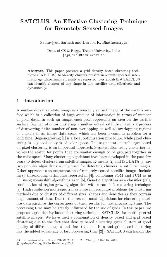
SATCLUS: An Effective Clustering Technique
for Remotely Sensed Images
Sauravjyoti Sarmah and Dhruba K. Bhattacharyya
Dept. of CS & Engg., Tezpur University, Indiasjs,[email protected]
Abstract. This paper presents a grid density based clustering tech-nique (SATCLUS) to identify clusters present in a multi spectral satel-lite image. Experimental results are reported to establish that SATCLUScan identify clusters of any shape in any satellite data effectively anddynamically.
1 Introduction
A multi-spectral satellite image is a remotely sensed image of the earth’s sur-face which is a collection of huge amount of information in terms of numberof pixel data. In such an image, each pixel represents an area on the earth’ssurface. Segmentation or clustering a multi-spectral satellite image is a processof discovering finite number of non-overlapping as well as overlapping regionsor clusters in an image data space which has been a complex problem for along time. Region-growing [1] is a local optimization procedure, while pixel clus-tering is a global analysis of color space. The segmentation technique basedon pixel clustering is an important approach. Segmentation using clustering in-volves the search for points that are similar enough to be grouped together inthe color space. Many clustering algorithms have been developed in the past fewyears to detect clusters from satellite images. K-means [2] and ISODATA [3] aretwo popular algorithms widely used for detecting clusters in satellite images.Other approaches to segmentation of remotely sensed satellite images includefuzzy thresholding techniques reported in [4], combining SOM and FCM as in[5], using mean-shift algorithms as in [6], Genetic algorithm as a classifier ([7]),combination of region-growing algorithm with mean shift clustering technique[8]. High resolution multi-spectral satellite images cause problems for clusteringmethods due to clusters of different sizes, shapes and densities as they containhuge amount of data. Due to this reason, most algorithms for clustering satel-lite data sacrifice the correctness of their results for fast processing time. Theprocessing time may be greatly influenced by the use of grids. In this paper, wepropose a grid density based clustering technique, SATCLUS, for multi-spectralsatellite images. We have used a combination of density based and grid basedclustering due to the fact that density based clustering gives clusters of goodquality of different shapes and sizes ([2], [9], [10]); and grid based clusteringhas the added advantage of fast processing time([2]). SATCLUS can handle the
S.O. Kuznetsov et al. (Eds.): PReMI 2011, LNCS 6744, pp. 110–115, 2011.c© Springer-Verlag Berlin Heidelberg 2011

SATCLUS: An Effective Clustering Technique for Remotely Sensed Images 111
detection of irregular shaped clusters by pixel level processing of the cluster bor-ders. Most region growing algorithms are executed in a left to right, top-downmanner, whereas SATCLUS initiates the cluster expansion process starting withthe maximum hue value. Due to the use of grid-based technique, SATCLUS isscalable even for large datasets. SATCLUS does not require the initial of clustercenters; neither does the number of clusters play any role in the clustering pro-cess. SATCLUS was tested on a large number of multi-spectral satellite imageryand the cluster results are found very satisfactory.
2 The Proposed Technique
The aim of our clustering algorithm is to discover clusters over multi spectralhigh resolution satellite images. Following definitions [11] provide the basis ofSATCLUS.
Definition 1. Difference value of a pixel w.r.t. the seed pixel is the distance(dist) between the HSI values of that pixel and the seed. If dist ≤ θ, then thedifference value of that pixel is considered as 1 otherwise 0, where dist, is anyproximity measure (here we have used Mahalanobis distance).
Definition 2. Population-object ratio is the ratio of the population count (num-ber of ones in each grid cell) and cell density (number of pixels within a particulargrid cell) of a grid cell, i.e., population count/ cell density
Definition 3. If the difference of the population-object ratio of the current celland one of its neighbors is greater than or equal to some threshold α then α isthe confidence between them. For two cells p and q to be merged into the samecluster the following condition should be satisfied:
α ≤| Po(p)−Po(q) |, and α = θ×Po(seed) where Po represents the population-object ratio of that particular cell and seed is the cell which initiates the expan-sion of a cluster.
Definition 4. Cell reachability: A cell p is reachable from a cell q if p is aneighbor cell of q and cell p satisfies the confidence condition w.r.t. cell q.
Definition 5. Rough cluster: A rough cluster is defined to be the set of pointsbelonging to the set of reachable cells. A rough cluster C w.r.t. α is a non-emptysubset satisfying the following condition,∀p, q: if p ∈ C and q is reachable from p w.r.t. α, then q ∈ C, where p and q arecells.
Definition 6. Border cell: A cell p is a border cell if it is part of a rough clusterCi and at least one of its neighbors is part of another rough cluster Cj.
Definition 7. Noise: Noise is simply the set of points belonging to the cells notbelonging to any of its clusters. Let C1, C2, · · ·Ck be the clusters w.r.t. α, thenNoise = no p | p ∈ n × n,∀i : no p /∈ Ci, where no p is the set of points incell p and Ci (i = 1, · · · , k).

112 S. Sarmah and D.K. Bhattacharyya
2.1 Procedure of SATCLUS
The algorithm starts with dividing the image space into n × n non-overlappingsquare grid cells, where n is a user input, and maps the image pixels to eachcell. It then calculates the density of each cell. Next, it converts the RGB valuesof each pixel to its corresponding HSI values. The algorithm uses the cell infor-mation (density) of the grid structure and clusters the data points according totheir surrounding cells. The clustering process is divided into two steps. In thefirst step a rough clustering of the image space is obtained and the second stepdeals with cluster smoothening for quality cluster identification. The executionof the rough clustering algorithm (Step I) includes the following steps:
Input: The Image dataset1. Create the grid structure.2. Compute the density of each cell.3. Convert the RGB values of each pixel into their HSI values.4. Identify the maximum hue value as the seed.5. Calculate each pixels difference value w.r.t. the seed.6. The population count of each grid cell is computed and the corresponding
population-object ratio calculated.7. Traverse the neighbor cells starting from the grid-cell having the highest
population-object ratio value.8. Merge the cells and assign cluster id.9. Repeat steps 5 through 9 till all cells are classified.
The value of θ mostly depends on the values of the h, s, i (i.e., hue, saturationand intensity) and the resolution of the image. However, based on our exhaustiveexperimentation over various multi-spectral and pan-chromatic satellite images,it has been observed that an effective range of θ for multi-spectral images is 15 ≤θ ≤ 30 and for pan-chromatic images, the range is found to be 0.5 ≤ θ ≤ 4.0. Therough clusters obtained in Step I are grainy in nature which is a drawback of agrid based algorithm. To obtain clusters with smooth and accurate borders, theborder cells are detected and re-clustered using a partitioning based approachas given in Step II. The algorithm for the cluster smoothening is given below:Input: q border cells; k seeds corresponding to the k rough clusters obtainedfrom Step I1. Start with an arbitrary border pixel x2. Find the distance of x to each of the k seeds3. Assign x to the cluster to which it has minimum distance w.r.t. the seed4. Repeat steps 1 to 3 till all border pixels have been reassigned
The partitioning of the dataset into n × n non-overlapping cells results in acomplexity of O(n×n). The complexity of rough clustering in step I is O(k×p),where p is the number of cells in a cluster so formed and p n × n in theaverage case and k is the number of clusters obtained. Similarly in step II, foridentification of the q border cells require O(q) times where q n × n andassignment of r pixels to k clusters requires O(k × r) times, where r is thetotal number of pixels in q cells. However, O(k × r) dominates the overall timecomplexity since n, p, q r.
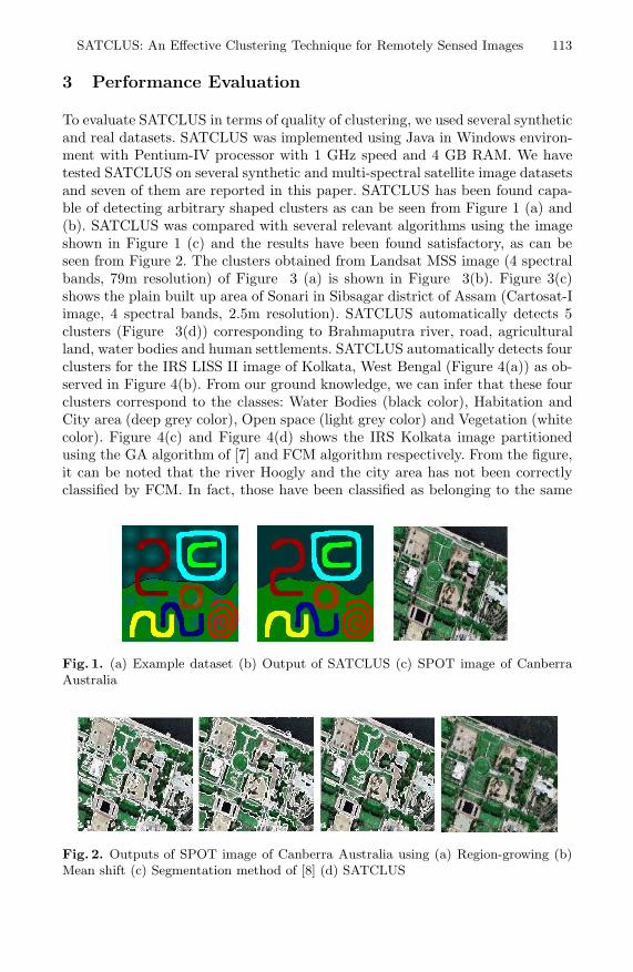
SATCLUS: An Effective Clustering Technique for Remotely Sensed Images 113
3 Performance Evaluation
To evaluate SATCLUS in terms of quality of clustering, we used several syntheticand real datasets. SATCLUS was implemented using Java in Windows environ-ment with Pentium-IV processor with 1 GHz speed and 4 GB RAM. We havetested SATCLUS on several synthetic and multi-spectral satellite image datasetsand seven of them are reported in this paper. SATCLUS has been found capa-ble of detecting arbitrary shaped clusters as can be seen from Figure 1 (a) and(b). SATCLUS was compared with several relevant algorithms using the imageshown in Figure 1 (c) and the results have been found satisfactory, as can beseen from Figure 2. The clusters obtained from Landsat MSS image (4 spectralbands, 79m resolution) of Figure 3 (a) is shown in Figure 3(b). Figure 3(c)shows the plain built up area of Sonari in Sibsagar district of Assam (Cartosat-Iimage, 4 spectral bands, 2.5m resolution). SATCLUS automatically detects 5clusters (Figure 3(d)) corresponding to Brahmaputra river, road, agriculturalland, water bodies and human settlements. SATCLUS automatically detects fourclusters for the IRS LISS II image of Kolkata, West Bengal (Figure 4(a)) as ob-served in Figure 4(b). From our ground knowledge, we can infer that these fourclusters correspond to the classes: Water Bodies (black color), Habitation andCity area (deep grey color), Open space (light grey color) and Vegetation (whitecolor). Figure 4(c) and Figure 4(d) shows the IRS Kolkata image partitionedusing the GA algorithm of [7] and FCM algorithm respectively. From the figure,it can be noted that the river Hoogly and the city area has not been correctlyclassified by FCM. In fact, those have been classified as belonging to the same
Fig. 1. (a) Example dataset (b) Output of SATCLUS (c) SPOT image of CanberraAustralia
Fig. 2. Outputs of SPOT image of Canberra Australia using (a) Region-growing (b)Mean shift (c) Segmentation method of [8] (d) SATCLUS
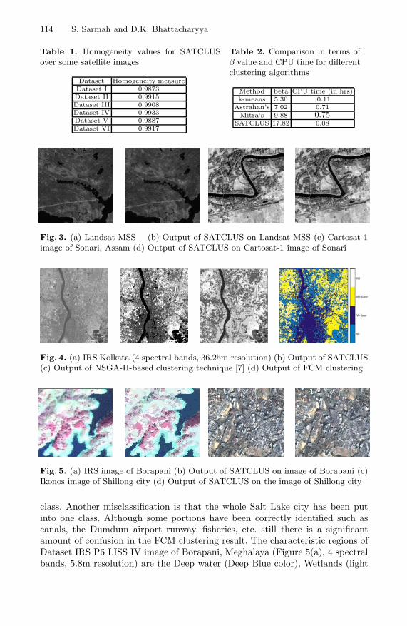
114 S. Sarmah and D.K. Bhattacharyya
Table 1. Homogeneity values for SATCLUSover some satellite images
Dataset Homogeneity measureDataset I 0.9873Dataset II 0.9915Dataset III 0.9908Dataset IV 0.9933Dataset V 0.9887Dataset VI 0.9917
Table 2. Comparison in terms ofβ value and CPU time for differentclustering algorithms
Method beta CPU time (in hrs)k-means 5.30 0.11
Astrahan’s 7.02 0.71Mitra’s 9.88 0.75
SATCLUS 17.82 0.08
Fig. 3. (a) Landsat-MSS (b) Output of SATCLUS on Landsat-MSS (c) Cartosat-1image of Sonari, Assam (d) Output of SATCLUS on Cartosat-1 image of Sonari
Fig. 4. (a) IRS Kolkata (4 spectral bands, 36.25m resolution) (b) Output of SATCLUS(c) Output of NSGA-II-based clustering technique [7] (d) Output of FCM clustering
Fig. 5. (a) IRS image of Borapani (b) Output of SATCLUS on image of Borapani (c)Ikonos image of Shillong city (d) Output of SATCLUS on the image of Shillong city
class. Another misclassification is that the whole Salt Lake city has been putinto one class. Although some portions have been correctly identified such ascanals, the Dumdum airport runway, fisheries, etc. still there is a significantamount of confusion in the FCM clustering result. The characteristic regions ofDataset IRS P6 LISS IV image of Borapani, Meghalaya (Figure 5(a), 4 spectralbands, 5.8m resolution) are the Deep water (Deep Blue color), Wetlands (light
SATCLUS: An Effective Clustering Technique for Remotely Sensed Images 115
blue color), Vegetation (Red and Pink colors) and Open spaces (White color).Executing SATCLUS on this image resulted in the detection of the above fourclasses as shown in Figure 5(b). The clustered image output obtained by SAT-CLUS on the IKONOS image of Shillong, Meghalaya (Figure 5(c), 4 spectralbands, resolution of 4m for multispectral and 1m for panchromatic imagery) isshown in Figure 5(d) which relate well with the ground information known tous (concrete structures, roads, open spaces, etc). The performance of SATCLUSin terms of homogeneity measure [2] for some satellite images is shown in Table1. SATCLUS has also been evaluated quantitatively using an index β [4] andthe results for Dataset II can be seen from Table 2. SATCLUS has the highestβ value in comparison to the comparable algorithms.
4 Conclusions and Future Work
The proposed SATCLUS was experimentally tested and found capable in detect-ing the clusters qualitatively and efficiently in light of several real-life satelliteimages. Work is going on to extend the SATCLUS algorithm for handling hype-rion (hyper spectral) data and also to extend the work using a fuzzy-rough setbased approach. As a future direction of our work, we a plan to experiment thetechnique on microwave remote sensing data.
References
1. Baatz, M., Schape, A.: Multiresolution segmentation: an optimization approachfor high quality multi-scale image segmentation. Journal of Photogrammetry andRemote Sensing 58(3-4), 12–23 (2000)
2. Han, J., Kamber, M.: Data Mining: Concepts and Techniques. Morgan KaufmannPublishers, San Fransisco (2004)
3. Ball, G.H., Hall, D.J.: A clustering technique for summarizing multivariate data.Behavioural Science 12, 153–155 (1967)
4. Pal, S.K., Ghosh, A., Shankar, B.U.: Segmentation with remotely sensed images withfuzzy thresholding and quantitative evaluation. IJRS 21(11), 2269–2300 (2000)
5. Awad, M.M., Nasri, A.: Satellite image segmentation using self- organizing mapsand fuzzy c-means. In: IEEE International Symposium on Signal Processing andInformation Technology (ISSPIT), pp. 398–402 (2009)
6. Comaniciu, D., Meer, P.: Robust analysis of feature spaces: Color image segmen-tation. In: Proc. of the IEEE Conf. on Computer Vision and Pattern Recognition(CVPR), pp. 750–755 (1997)
7. Bandyopadhyay, S., Maulik, U., Mukhopadhyay, A.: Multiobjective genetic clus-tering for pixel classification in remote sensing imagery. TGRS 45(2), 1506–1511(2007)
8. Bo, S., Ding, L., Jing, Y.: On combining region-growing with non-parametric clus-tering for color image segmentation. In: CISP, pp. 715–719 (2008)
9. Astrahan, M.M.: Speech analysis by clustering, or the hyper-phoneme method.Stanford A. I. Project Memo (1970)
10. Mitra, P., Murthy, C.A., Pal, S.K.: Density-based multiscale data condensation.IEEE TPAMI 24(6) (June 2002)
11. Sarmah, S., Das, R., Bhattacharyya, D.K.: A distributed algorithm for intrinsiccluster detection over large spatial data. IJCS 3(4), 246–256 (2008)

Blur Estimation for Barcode Recognition in
Out-of-Focus Images
Duy Khuong Nguyen, The Duy Bui, and Thanh Ha Le
Human Machine Interaction LaboratoryUniversity Engineering and Technology
Vietnam National University, Hanoikhuongnd,duybt,[email protected]
Abstract. Recently, with the popularity of hand-held devices with cam-era, many applications requiring barcode identification in images haveappeared. There are several problems with these applications because ofthe limitation of camera capability. Among them, heavily blur problemsare the most significant and popular. In this paper, we propose a novelapproach to estimate blur for recognising barcodes in heavily blurredimages. With this approach, we are able to extract correctly the barcodefrom heavily blurred images, which existing methods cannot.
Keywords: Blur estimation, Barcode identification, pattern recogni-tion, heavily blurred images.
1 Introduction
Recently, with the popularity of mobile phones aimed with integrated camera,there is a need for recognising barcodes from images captured from these de-vices. However, due to the limitation of controlling focus lens, the capturedimages are often heavily distorted by the out of focus blur. Therefore, it is veryhard to extract the barcode from these heavily distorted images with existingmethods proposed for conventional barcode reader. There are several approachesreported in literature for solving the blur problem in barcode recognition, e.g.edge detection-based approach [3,5,6], inverse-problem-based approach [2] andstatistical machine learning techniques[7]. These techniques cannot work wellfor heavily distorted signals [7] because it is difficult to extract features such asedges and peaks of the bars and spaces from these signals.
In this paper, we propose a novel approach to estimate blur for recognisingbarcodes in heavily blurred images. We first estimate the ranges of blur param-eters, and then search through these ranges with sampled values to find theparameters that allow us to extract correctly the most number of barcode val-ues along the scan lines of the barcode image. For each scan line, we generatecandidate signals by utilising the structure of the barcode, blur them with blurparameters in process, and compare with the distorted signal of the scan line tofind the best matched candidate signal. The checksum of the barcode is used to
S.O. Kuznetsov et al. (Eds.): PReMI 2011, LNCS 6744, pp. 116–121, 2011.c© Springer-Verlag Berlin Heidelberg 2011

Blur Estimation for Barcode Recognition in Out-of-Focus Images 117
verify the candidate. With this approach, we are able to extract correctly thebarcode from heavily blurred images, which existing methods cannot.
The paper is organised as follows. In Section 2, barcode representation isdescribed in details. The emphasis of the paper is in Section 3 which presentsrelated works. Subsequently, our proposed algorithm in Section 4 is followed byexperiments and results in Section 5.
2 Barcode Signal Reconstruction
From a 2D image of the barcode, a unique 1D signal can be extracted by scanninga horizontal line through the barcode image. Therefore, the barcode can berepresented as a series of 1D patterns representing 0s and 1s (see Fig. 1):
S = u(x) ∈ L2(R) : u(x) ∈ 0, 1 (1)
If the signal obtained from the image looks sharp and clear like in Fig. 1,the barcode can be recognised easily. However, as the captured barcode imageis blurred and noised as in Fig. 2, the extracted 1D signal is heavily distorted(see Fig. 2). In this case, it is very hard to recognise the barcode precisely.
Fig. 1. Clear barcode image and orginal signals
Fig. 2. Blurred barcode image and blurred signals
The sharpness of the captured signal depends on the reader device and itsdistance between the reader and the surface of barcode. The longer the distancebetween them, the more blurred the original signal is. The blurred signal f(x) isoften modelled as the noise added convolution of the original signal u(x) with aGaussian kernel of unknown amplitude α and standard deviation σ [2]:
f(x) = α ∗ Gσ ∗ u(x) + n(x) (2)

118 D.K. Nguyen, T.D. Bui, and T.H. Le
where n(x) is a noise function, α is a strictly positive constant, and
Gσ =1
σ√
2π∗ e−
x2
2σ2 (3)
3 Related Works
In the approach based on edge detection, traditional barcode decoding tech-niques such as peak locations [3], selective sampling [5] and EM algorithm [6]have been employed. These approaches cannot work well if the phone camerasare designed with low quality [7] or the images are heavily distorted. In fact, withhandheld cameras, noises and focusing errors may appear frequently. In otherwords, it is really difficult to extract features such as edges and peaks of the barsand spaces from the heavily distorted images. In another approach, barcode isextracted after the process of signal restoration through solving an inverse prob-lem [2]. There are two serious problems with this approach. Firstly, restoredsignals usually have errors because the degrading process is often unknown andcomplex. Secondly, the cost of computation is considerably high because of theprocess of signal restoration. Finally, this approach is only suitable with simu-lated images. For real images, barcode cannot be recognised correctly. Besidestwo above approaches, statistical machine learning techniques [7] are also usedto identify barcode. Based on the nature of the contaminated barcode symbols,the trained classifiers are able to discriminate different code patterns by extract-ing their statistical features [7]. However, the cost for maintaining the system isconsiderably high because collecting training data is often an absolutely greattask. In addition, each type of barcode or a change of capturing device needs aparticular recognition system.
4 Our Proposed Approach
To recognise barcode patterns in heavily distorted images, we propose an effectivealgorithm in both of accuracy and performance, in which the prior structuralknowledge of barcode is used thoroughly.
Despite that images may be distorted, barcodes can be located quite easilybecause of several reasons: they contains black and white vertical lines and everybarcode have less than four consecutive 1s or 0s; they are often printed in sep-arated area; and they often have the ratio of 3:4 between the height and width.After locating the barcode in the distorted image, we estimate the blur param-eters. This is done by comparing the size of the barcode in the distorted imagewith the actual size of a barcode and locating the position of two border guardbars by optimising the error function. Blurred signals of digits are pre-computedwith the estimated blur parameters. This pre-computation is conducted in orderto speed up our algorithm. We then go through each scan line of the barcodeimage to find the barcode value that that best matches the signal of scan line.This is done by first re-locating the guard bars, calculating position of each digit

Blur Estimation for Barcode Recognition in Out-of-Focus Images 119
input : A heavily distorted image containing a barcodeoutput: The value encoded in the barcode
Locate the rectangle containing the barcode;Estimate blur parameters via locating border guard bars;Compute blurred signals of digits;foreach line of horizontal scan lines of the barcode image do
re-locate the guard bars of barcode;stretch signals of barcode with pixels per bit equal toGaussian kernel size/2 + 1;foreach position of surrounding positions of left border do
foreach digit of left digits dochoose the digit having minimum function;move left boder to the next position of the best pattern;
end
enddetermine the first digit based on the left digit code;do similarly for the right digits;reconstruct the whole of barcode;if checksum of the found barcode value is true then
the barcode value is added as a voteend
endif the maximal number of vote for a barcode exceed a threshold then
return the barcode value is added as a vote;endelse
return that barcode cannot be recognised;end
Algorithm 1. Pseudo-code for barcode recognition algorithm
in the barcode and comparing the signal of the scan line with blurred signals ofdigits. The first digit is implied by the patterns of six left digits. If the checksumof the detected value of the barcode is true, the barcode value is added as a vote.The barcode value with maximal number of vote is returned as result. The verydetail of barcode recognition process is explained in Algorithm 1.
4.1 The Error Function
The error function that we use when finding the best matched candidate for eachconsidered pattern is as follows:
E = ||f(x) − α • Gσ ∗ u(x)|| (4)
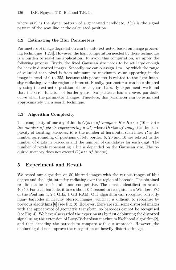
120 D.K. Nguyen, T.D. Bui, and T.H. Le
where u(x) is the signal pattern of a generated candidate, f(x) is the signalpattern of the scan line at the calculated position.
4.2 Estimating the Blur Parameters
Parameters of image degradation can be auto-extracted based on image process-ing techniques [1,2,4]. However, the high computation needed by these techniquesis a burden to real-time application. To avoid this computation, we apply thefollowing process. Firstly, the fixed Gaussian size needs to be set large enoughfor heavily distorted images. Secondly, we can α assign 1 to , by which the rangeof value of each pixel is from minimum to maximum value appearing in theimage instead of 0 to 255, because this parameter is related to the light inten-sity radiating over the region of interest. Finally, parameter σ can be estimatedby using the extracted position of border guard bars. By experiment, we foundthat the error function of border guard bar patterns has a convex paraboliccurve when the parameter changes. Therefore, this parameter can be estimatedapproximately via a search technique.
4.3 Algorithm Complexity
The complexity of our algorithm is O(size of image + K ∗ R ∗ 6 ∗ (10 + 20) ∗the number of pixels representing a bit) where O(size of image) is the com-plexity of locating barcodes. K is the number of horizontal scan lines. R is thenumber surrounding of positions of left border. 6, 20 and 10 are related to thenumber of digits in barcodes and the number of candidates for each digit. Thenumber of pixels representing a bit is depended on the Gaussian size. The re-quired memory does not exceed O(size of image).
5 Experiment and Result
We tested our algorithm on 50 blurred images with the various ranges of blurdegree and the light intensity radiating over the region of barcode. The obtainedresults can be considerable and competitive. The correct identification rate is46/50. For each barcode, it takes about 0.5 second to recognise in a Windows PCof the Pentium 4, 2.4 GHz, 1 GB RAM. Our algorithm can recognise correctlymany barcodes in heavily blurred images, which it is difficult to recognise byprevious algorithms [6] (see Fig. 3). However, there are still some distorted imageswith the appearance of geometric transform, so barcodes cannot be recognised(see Fig. 4). We have also carried the experiments by first deblurring the distortedsignal using the extension of Lucy-Richardson maximum likelihood algorithm[2],and then decoding the barcode to compare with our approach. However, thedeblurring did not improve the recognition on heavily distorted image.
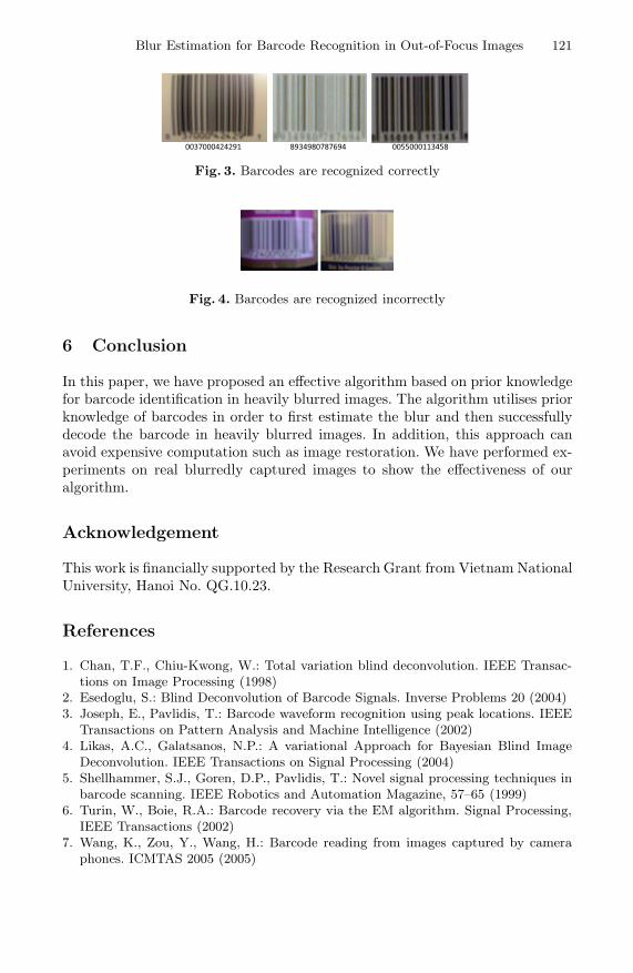
Blur Estimation for Barcode Recognition in Out-of-Focus Images 121
Fig. 3. Barcodes are recognized correctly
Fig. 4. Barcodes are recognized incorrectly
6 Conclusion
In this paper, we have proposed an effective algorithm based on prior knowledgefor barcode identification in heavily blurred images. The algorithm utilises priorknowledge of barcodes in order to first estimate the blur and then successfullydecode the barcode in heavily blurred images. In addition, this approach canavoid expensive computation such as image restoration. We have performed ex-periments on real blurredly captured images to show the effectiveness of ouralgorithm.
Acknowledgement
This work is financially supported by the Research Grant from Vietnam NationalUniversity, Hanoi No. QG.10.23.
References
1. Chan, T.F., Chiu-Kwong, W.: Total variation blind deconvolution. IEEE Transac-tions on Image Processing (1998)
2. Esedoglu, S.: Blind Deconvolution of Barcode Signals. Inverse Problems 20 (2004)3. Joseph, E., Pavlidis, T.: Barcode waveform recognition using peak locations. IEEE
Transactions on Pattern Analysis and Machine Intelligence (2002)4. Likas, A.C., Galatsanos, N.P.: A variational Approach for Bayesian Blind Image
Deconvolution. IEEE Transactions on Signal Processing (2004)5. Shellhammer, S.J., Goren, D.P., Pavlidis, T.: Novel signal processing techniques in
barcode scanning. IEEE Robotics and Automation Magazine, 57–65 (1999)6. Turin, W., Boie, R.A.: Barcode recovery via the EM algorithm. Signal Processing,
IEEE Transactions (2002)7. Wang, K., Zou, Y., Wang, H.: Barcode reading from images captured by camera
phones. ICMTAS 2005 (2005)

S.O. Kuznetsov et al. (Eds.): PReMI 2011, LNCS 6744, pp. 122–129, 2011. © Springer-Verlag Berlin Heidelberg 2011
Entropy-Based Automatic Segmentation of Bones in Digital X-ray Images
Oishila Bandyopadhyay1, Bhabatosh Chanda2, and Bhargab B. Bhattacharya2
1 Department of CSE, Camellia Institute of Technology, Kolkata -700129, India 2 Center for Soft Computing Research, Indian Statistical Institute, Kolkata - 700 108, India
Abstract. Bone image segmentation is an integral component of orthopedic X-ray image analysis that aims at extracting the bone structure from the muscles and tissues. Automatic segmentation of the bone part in a digital X-ray image is a challenging problem because of its low contrast with the surrounding flesh, which itself needs to be discriminated against the background. The presence of noise and spurious edges further complicates the segmentation. In this paper, we propose an efficient entropy-based segmentation technique that integrates several simple steps, which are fully automated. Experiments on several X-ray images reveal encouraging results as evident from a segmentation entropy quantitative assessment (SEQA) metric [Hao, et al. 2009].
Keywords: Entropy, Digital X-ray, LOCO, Medical imaging, Segmentation.
1 Introduction
Segmentation of an anatomical object from an X-ray, MRI or a CT-scan image is a challenging task as the intensity values of the region-of-interest and the surrounding region are very close, and the contour clarity is often low. Many traditional image segmentation approaches are computationally intensive or need manual intervention [1, 2].
In last two decades, numerous segmentation models and algorithms for analyzing various classes of medical images have been reported. The selection of proper segmentation method is another important issue as this choice widely depends on specific application, image modality and several other factors [1, 2]. In this paper, we briefly discuss some notable segmentation algorithms used in medical imaging and then propose an integrated entropy-based technique suitable for bone segmentation in a digital X-ray image from the surrounding flesh region. The method is simple and fully automated and it uses a new thresholding parameter. The quality of segmentation is observed to outperform those obtained by several earlier methods [3, 13] as indicated by the segmentation entropy quantitative assessment (SEQA) [16].
2 Medical Image Segmentation: Prior Art
Image segmentation is defined as its partitioning into different parts, which are homogenous in nature with respect to some characteristics. The region-of-interest

Entropy-Based Automatic Segmentation of Bones in Digital X-ray Images 123
(ROI) may be a complete object or a part of it [2, 5]. Medical image segmentation algorithms can be classified into categories like those based on analysis of edges, regions, pixel classification, graphs, or on deformable model, fuzzy logic, artificial neural network, statistical or morphological approaches. The segmentation algorithms based on region analysis or pixel classification, make use of the homogeneity in the image, whereas the edge detection and graph-based algorithms perform segmentation by detecting any abrupt change in the image within a small neighborhood [5]. The Canny edge detector uses two levels of thresholding. Šćepanović et al. adopted Canny’s method for probabilistic bone edge detection [6].
The deformable model based approaches allow elastic decomposition of the objects by incorporating concepts of continuum mechanics. The active contour or snake model was proposed by Kass et al. [7]. In deformable models like snake, the user provides an initial guess of contour of ROI, which is then moved by the image-driven forces to the boundary of the desired object. However, the snake method with gradient vector flow (GVF) has slow convergence on irregular objects with high concavities like X-ray images of deformed bone structure.
The active shape model and active appearance model are also used in medical image segmentation. Unfortunately, both the methods require large training samples to build a point distribution in the high-dimensional eigen space. The statistical models like probability distribution map and Markov random field model have also been used widely for medical image segmentation. Liang et al. have used statistical and morphology based technique for fracture identification in an X-ray image [19]. Pal et al. [10] studied segmentation of MRI samples using fuzzy-based approaches.
Several semi-automatic image segmentation methods incorporate user interaction and allow the user to mark the ROI or background objects roughly on the image. Ning et al. proposed an interactive image segmentation algorithm based on maximal similarity based region merging [12].
Thresholding-based segmentation approaches are widely used in medical image analysis [8, 9]. Sen et al. proposed a method based on gradient histogram and applied it on a chest X-ray image among others [8].Yan et al. used an entropy-based thresholding approach for segmentation of bacteria images from a low intensity background [13]; however, this method requires a tuning parameter, which is chosen based on experience.
3 Proposed Approach for X-ray Image Segmentation
In an X-ray image, the bone parts appear along with the surrounding tissues or muscles (i.e. flesh) image. In many regions of an X-ray image, the intensity range of pixels belonging to the bone region and that of its surrounding flesh region may overlap, which makes the segmentation inaccurate. The bone region of an X-ray image is to be extracted out of two distinct background components, the image background and the overlapping flesh region. Thus, bone segmentation from the flesh region using pixel based thresholding or edge based approaches often do not produce accurate results.
In this paper, we have proposed a new entropy-based approach, which instead of direct entropy thresholding [13], first produces an intermediate image from the entropy matrix and then uses intensity-thresholding for segmenting the bone region in an X-ray

124 O. Bandyopadhyay, B. Chanda, and B.B. Bhattacharya
image. Finally, for contour correction, multilevel LOCO (Linear combination of Open-Close and Close-Open) filtering methods [11] are used.
3.1 Integrated Segmentation Algorithm
In the proposed algorithm, the transition regions in an input image are identified using entropy analysis and a gray scale entropy image is generated. This entropy image is used to compute the threshold value required for segmentation.
A high entropy value represents the presence of maximum information, i.e., higher gray value pixels in the image. An image with a very low entropy value represents noise with no meaningful information. The overlapping flesh and bone regions in an X-ray image cause the presence of a large number of pixels with similar intensity values. Computation of local entropy values of each pixel in a window helps to group the pixels with similar intensity values with a marked transition region. As a bone region has higher intensity values than those in the flesh region in an X-ray image, the transition boundaries are accentuated in the entropy image. The steps of the proposed algorithm are summarized below, details of which are elaborated subsequently.
Step 1: Convert an input X-ray image to a gray scale image.
Step 2: Perform entropy computation of each image pixel around (9×9) neighbors. For pixels at the border of the image, symmetric padding is used where the padded pixels are obtained by mirror reflection of the border pixels of the image.
Step 3: Generate an entropy image by converting the entropy matrix to a gray scale image, where the maximum entropy value is mapped to 255 and the minimum entropy value is mapped to 0. Other entropy values are linearly scaled between 0 and 255.
Step 4: Apply median filter on the entropy image.
Step 5: Compute the intensity threshold value for binarization of the entropy image.
Step 6: Produce the segmented bone image.
Step 7: Apply multilevel LOCO filter to enhance the contour of the segment.
3.2 Entropy Computation and Constructing Entropy Image
The entropy value represents the measure of randomness associated with pixel values belonging to each gray level. Following Shannon’s definition of entropy and Pun’s representation of image entropy, for an image with G gray levels, and probability of k-th gray level Pk, the image entropy can be represented as
E= ∑−
=
1
0
G
k
Pklog2(1/Pk) = - ∑−
=
1
0
G
k
Pklog2(Pk) (1)
where Pk = nk/M×N , nk is the number of pixels with grayscale k and M×N is the size of the image [5].
Local entropy represents the discrepancy between two probability distributions on the same event space [13]. It is related to the variance of grayscales in the neighborhood
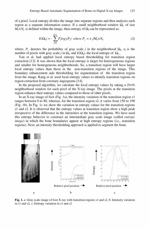
Entropy-Based Automatic Segmentation of Bones in Digital X-ray Images 125
of a pixel. Local entropy divides the image into separate regions and then analyzes each region as a separate information source. If a small neighborhood window Ωk of size Mk×Nk is defined within the image, then entropy of Ωk can be represented as:
E(Ωk) = - ∑−
=
1
0
G
j
Pjlog2(Pj) where Pj = n j/Mk×Nk (2)
where, Pj denotes the probability of gray scale j in the neighborhood Ωk, nj is the number of pixels with gray scale j in Ωk, and E(Ωk), the local entropy of Ωk..
Yan et al. had applied local entropy based thresholding for transition region extraction [13]. It was shown that the local entropy is larger for heterogeneous regions and smaller for homogeneous neighborhoods. So, a transition region will have larger local entropy values than those in the non-transition regions of the image. This boundary enhancement aids thresholding for segmentation of the transition region from the image. Kang et al. used local entropy values to identify transition regions on region extraction from coronary angiograms [14].
In the proposed algorithm, we calculate the local entropy values by taking a (9×9) neighborhood window for each pixel of the X-ray image. The pixels at the transition region enhance their entropy values compared to those of other pixels.
In an X-ray image of foot (Fig. 1a), the intensity variation of the transition region s1 ranges between 0 to 80, whereas, for the transition region s2, it varies from 150 to 190 (Fig. 1b). In Fig. 1c we show the variation in entropy values for the transition regions s1 and s2. It is observed that the entropy values at transition region show a high peak irrespective of the difference in the intensities at the transition regions. We have used this entropy behavior to construct an intermediate gray scale image (called entropy image) in which the bone boundaries appear at high entropy regions (i.e., transition regions). Next, an intensity thresholding approach is applied to segment the bone.
a b c
Entro
py
Inte
nsity
Relative pixel position Relative pixel position
Fig. 1. a: Gray scale image of foot X-ray with transition regions s1 and s2, b: Intensity variation in s1 and s2, c: Entropy variation in s1 and s2
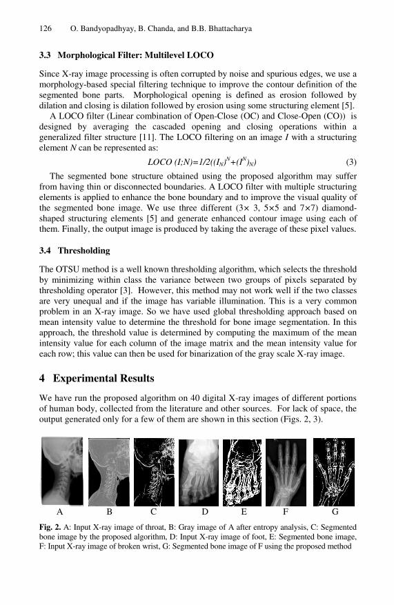
126 O. Bandyopadhyay, B. Chanda, and B.B. Bhattacharya
3.3 Morphological Filter: Multilevel LOCO
Since X-ray image processing is often corrupted by noise and spurious edges, we use a morphology-based special filtering technique to improve the contour definition of the segmented bone parts. Morphological opening is defined as erosion followed by dilation and closing is dilation followed by erosion using some structuring element [5].
A LOCO filter (Linear combination of Open-Close (OC) and Close-Open (CO)) is designed by averaging the cascaded opening and closing operations within a generalized filter structure [11]. The LOCO filtering on an image I with a structuring element N can be represented as:
LOCO (I;N)=1/2((IN)N+(IN)N) (3)
The segmented bone structure obtained using the proposed algorithm may suffer from having thin or disconnected boundaries. A LOCO filter with multiple structuring elements is applied to enhance the bone boundary and to improve the visual quality of the segmented bone image. We use three different (3× 3, 5×5 and 7×7) diamond-shaped structuring elements [5] and generate enhanced contour image using each of them. Finally, the output image is produced by taking the average of these pixel values.
3.4 Thresholding
The OTSU method is a well known thresholding algorithm, which selects the threshold by minimizing within class the variance between two groups of pixels separated by thresholding operator [3]. However, this method may not work well if the two classes are very unequal and if the image has variable illumination. This is a very common problem in an X-ray image. So we have used global thresholding approach based on mean intensity value to determine the threshold for bone image segmentation. In this approach, the threshold value is determined by computing the maximum of the mean intensity value for each column of the image matrix and the mean intensity value for each row; this value can then be used for binarization of the gray scale X-ray image.
4 Experimental Results
We have run the proposed algorithm on 40 digital X-ray images of different portions of human body, collected from the literature and other sources. For lack of space, the output generated only for a few of them are shown in this section (Figs. 2, 3).
A B C D E F G
Fig. 2. A: Input X-ray image of throat, B: Gray image of A after entropy analysis, C: Segmented bone image by the proposed algorithm, D: Input X-ray image of foot, E: Segmented bone image, F: Input X-ray image of broken wrist, G: Segmented bone image of F using the proposed method
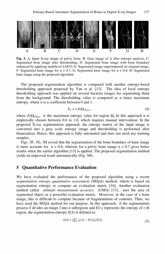
Entropy-Based Automatic Segmentation of Bones in Digital X-ray Images 127
A B C D E F G H
Fig. 3. A: Input X-ray image of pelvic bone, B: Gray image of A after entropy analysis, C: Segmented bone image after thresholding, D: Segmented bone image with bone boundary enhanced by applying multilevel LOCO, E: Segmented image superimposed on original image, F: Segmented knee image for α = 0.7, G: Segmented knee image for α = 0.8, H: Segmented knee image using the proposed algorithm
The proposed segmentation algorithm is compared with another entropy-based thresholding approach proposed by Yan et al. [13]. The idea of local entropy thresholding approach was applied on several bacteria images for segmenting them from the background. The thresholding value is computed as α times maximum entropy, where α is a coefficient between 0 and 1.
ET = α E(Ωk)max , (4)
where E(Ωk)max is the maximum entropy value for region Ωk..In this approach α is empirically chosen between 0.6 to 1.0, which requires manual intervention. In the proposed X-ray segmentation approach, the entropy matrix of the input image is converted into a gray scale entropy image and thresholding is performed after binarization. Hence, this approach is fully automated and does not need any training samples.
Figs. 3F, 3G, 3H reveal that the segmentation of the bone boundary of knee image is more accurate for α = 0.8, whereas for a pelvic bone image α = 0.7 gives better results when the earlier algorithm [13] is applied. The proposed segmentation method yields an improved result automatically (Fig. 3H).
5 Quantitative Performance Evaluation
We have evaluated the performance of the proposed algorithm using a recent segmentation entropy quantitative assessment (SEQA) method, which is based on segmentation entropy to compute an evaluation metric [16]. Another evaluation method called ultimate measurement accuracy (UMA) [17], uses the area of segmented object as a powerful evaluation metric. However, in the case of a bone image, this is difficult to compute because of fragmentation of contours. Thus, we have used the SEQA method for our purpose. In this approach, if the segmentation process S divides an image I into n subregions and E(ri) represents the entropy of ri th region, the segmentation entropy E(S) is defined as:
E(S) = (5)

128 O. Bandyopadhyay, B. Chanda, and B.B. Bhattacharya
where E(I) represents the total entropy of the original image.The segmentation entropy E(S) measures how much the image entropy changes during segmentation. Better segmented regions will be more homogeneous in nature and thus they will have lower region entropy. If the same image is segmented using two different segmentation algorithms A and B, and if E(A) is smaller than E(B), then according to Eqn (5), the performance of A is better than that of B [16].We have compared the segmentation entropy E of the proposed method with those of OTSU thresholding [3] and entropy thresholding [13]. These values for different digital X-ray images as listed in Table 1 support the effectiveness of the algorithm.
Table 1. Computation of segmentation entropy for some digital X-ray images
Image file E(S)
for OTSU E(S) for entropy
thresholding; α = 0.7 E(S) for
proposed method
Finger-Left.jpg (Fig. 2F) 3.52 2.63 2.05
Foot.jpg (Fig. 2D) 2.09 0.80 0.83
Leg.jpg (Fig. 3F) 2.48 1.92 1.48
Pelvic Bone.jpg (Fig. 3A) 1.77 0.82 0.77
Throat.jpg (Fig. 2A) 1.11 0.30 0.28
6 Discussion and Conclusion
We have developed an entropy-based X-ray image segmentation technique for bone part extraction. This is based on automatic thresholding of an entropy image defined by the entropy values in a neighborhood window of the given image. It has been observed that in many cases the bone boundary becomes fragmented after thresholding. To overcome this problem, we have applied a multilevel-averaging LOCO filter to enhance the bone contour of the segmented image. The method is fully automated and has superior performance over two earlier methods as evident by the SEQA metric. This algorithm will be useful for fracture detection in an X-ray image where, separation of bone from the surrounding flesh is needed for further analysis.
Acknowledgment. Some of the digital X-ray images were supplied by Dr. A. R. Sikdar and Sudarshan Polyclinic, Kolkata. We thankfully acknowledge their support.
References
1. Sezgin, M., Sankur, B.: Survey over image thresholding techniques and quantitative performance evolution. Journal of Electronic Imaging 13(1), 146–165 (2004)
2. Pham, D.L., Xu, C., Prince, J.L.: A survey of current methods in medical image segmentation. Annual Review of Biomedical Engineering 2, 315–337 (1998)
3. Otsu, N.: A threshold selection method from gray-level histograms. IEEE Transactions on Systems, Man and Cybernetics 9, 62–66 (1979)
Entropy-Based Automatic Segmentation of Bones in Digital X-ray Images 129
4. Yang, J., Staib, L.H., Duncan, V.: Neighborhood-constrained segmentation with level based 3-D deformable models. IEEE Transactions on Medical Imaging 23(8), 940–948 (2004)
5. Gonzalez, R.C., Woods, R.E.: Digital Image Processing. Pearson, London (2008) 6. Šćepanović, D., Kirshtein, J., Jain, A.K., Taylor, R.H.: Fast algorithm for probabilistic
bone edge detection (FAPBED). In: SPIE, vol. 5747, pp. 1753–1765 (2005) 7. Kass, M., Witkin, A., Terzopoulos, D.: Snakes: Active contour models. International
Journal of Computer Vision 1(4), 321–331 (1988) 8. Sen, D., Pal, S.K.: Gradient histogram thresholding in a region of interest for edge
detection. Image and Vision Computing 28, 677–695 (2010) 9. Kundu, M.K., Pal, S.K.: Thresholding for edge detection using human psycho-visual
phenomena. Pattern Recognition Letters 4(6), 433–441 (1986) 10. Pal, S.K., King, R.A.: On edge detection of X-ray images using fuzzy set. IEEE
Transactions on Pattern Analysis and Machine Intelligence 5, 69–77 (1983) 11. Schulze, M.A., Pearce, J.A.: Linear combinations of morphological operators: The
midrange, pseudomedian, and LOCO filters. In: IEEE International Conference on Acoustics, Speech, and Signal Processing, pp. 57–60 (1993)
12. Ning, J.L., Zhang, J., Zhang, D., Wu, C.: Interactive image segmentation by maximal similarity based region merging. Pattern Recognition 43, 445–456 (2010)
13. Yan, C., Sang, N., Zhang, T.: Local entropy-based transition region extraction and thresholding. Pattern Recognition Letters 24, 2935–2941 (2003)
14. Kang, W., Wang, K., Wang, Q., An, D.: Segmentation method based on transition region extraction for coronary angiograms. In: IEEE International Conference on Mechatronics and Automation, pp. 905–909 (2009)
15. Pal, N.R., Pal, S.K.: A review on image segmentation techniques. Pattern Recognition 23(9), 1277–1294 (1993)
16. Hao, J., Shen, Y., Xu, H., Zou, J.: A region entropy based objective evaluation method for image segmentation. In: IEEE International Conference on Instrumentation and Measurement Technology, pp. 373–377 (2009)
17. Zhang, Y.: A survey on evaluation methods for image segmentation. Pattern Recognition 29(8), 1335–1346 (1996)
18. Ding, F.: Segmentation of bone structure in X-ray images. Thesis Proposal, School of Computing, National University of Singapore (2006)
19. Liang, J., Pan, B.-C., Fan, Y.-H.: Fracture identification of X-ray image. In: International Conference on Wavelet Analysis and Pattern Recognition, pp. 67–73 (2010)
Principle and Method of Image Recognition
under Diffusive Distortions of Image
Jaser Doroshenko1, Lev Dulkin1, Viktor Salakhutdinov2, and Yury Smetanin3
1 Central Clinical Hospital of the Russian Academy of Sciences, Litovsky boul. 1a,119333, Moscow, Russia
retinaretina.ru2 Research Institute of System Investigations of the Russian Academy of Sciences,
Nahimovsky av.36-1, 117218, Moscow, Russiavsalakhutdinovgmail.com
3 Computer Center of the Russian Academy of Sciences, Vavilov st. 40, 119333,Moscow, Russiasmetaninrfbr.ru
Abstract. The results of investigation and development of software andhardware tools for processing images of ring objects under diffusive dis-sipation are presented. The proposed algorithm was demonstrated to beefficient in endoscopy for measuring the sizes of biological objects. Aprincipal scheme of a hardware system for the implementation of thenew method is presented. A plan of clinical testing of the new system isdeveloped.
Keywords: evidence-based medicine, biomedical informatics, imagerecognition, endoscope, measurement algorithm.
1 Introduction
One of the most important topics in evidence-based medicine is the objectiveevaluation of the quality of clinical research. Practice demonstrates that manycontemporary methods of measuring do not meet the requirements of evidence-based medicine. That is especially true for medical image processing and analysis.
The importance of endoscopic images in medicine is the consequence of thefact that now they are the main, and sometimes the only possible source of infor-mation for noninvasive visualization of internal anomalies and for the diagnosticsof various diseases [1]. The implementation of the endoscopic imaging is basedon small size TV systems that are inserted into the investigated region. If thesize is large, mosaicking is necessary.
The most important deadlock is that modern endoscopic methods and systemsdo not measure the distance between the camera and the object, therefore, it isimpossible to match visible sizes of the objects in the image to their real size.The error in the estimation of the distance inevitably causes a wrong estimationof the size of the pathology, and as a consequence, a wrong strategic selectionof treatment. In practice, the error of measurement in traditional endoscopic
S.O. Kuznetsov et al. (Eds.): PReMI 2011, LNCS 6744, pp. 130–135, 2011.c© Springer-Verlag Berlin Heidelberg 2011

Principle and Method of Image Recognition 131
methods in some cases (e.g., in urologic checkup) is up to 3 to 5 times higherthan it is needed for the selection of the adequate strategy of treatment [4]. Itreduces the efficiency of endoscopic monitoring and diagnostics in TV medicine.
Below, we consider an approach to solving this problem that is based onscaling using test images with a priori known sizes. A light spot is projected ontothe image of the object. The size of the projection is used for the estimation of thescaling factor of the pathologies. The approach is well known and extensivelyused [5,6], but is precision is limited. In all practical implementations of theapproach, difficulties appear that are related to great aberrations of the opticalsystem of the endoscope [7]. Moreover, light dispersion occurs in a biologicaltissue which results in blurring and incorrect scaling.
A new system is proposed for imaging and processing. The system makes itpossible to evaluate the real size of the pathologies using their endoscopic images.It is also possible to evaluate the errors caused by the light dispersion and tocorrect them.
2 Principle and Methods
The measuring system consists of a PC, TV endoscope whose brightening sub-system uses an inertia-free light-emitting diode, and light fibers. At one end, alaser light source is situated, at the other, micro collimator, which gives at theoutput a light beam whose section is equal along the whole length.
The light fiber is situated in the instrumental channel of the endoscope in sucha way that it is possible to measure the direction of the laser beam by standardmanipulators fixed at the distal end of the endoscope. This solution makes itpossible to use optical systems with various angles between their optical axisand the axis of the instrumental channel (Fig. 1).
Microcollimator situated at the end of the light fiber transforms the divergentlight beam into the beam with constant section. The PC controls the light-emitting diode used as the light source, the laser at the input of the light fiber,and the image processing for the TV endoscope.
The object whose size is measured is placed near the center of the image.After receiving the signal:
1. A current image of the object near the center is registered in the operatingmemory and displayed at the monitor as a static frame.
2. Along the foreground of the pulse of the frame synchronization for the TVendoscope, the light-diode source at the input of the light fiber is switched on.
3. The next frame, which consists of the image of the projection of the colli-mated laser beam light onto the measured object, is registered in the operatingmemory.
4. As the result of the image processing (step 3), the section of the laser beamis quantified (in pixels).
5. In the static image, a line is manually marked whose size is to be measured.The length of the line is defined as its size in pixels divided by the size in pixels

132 J. Doroshenko et al.
Fig. 1. The principal scheme of the distal end of the endoscope
Fig. 2. Various halos around the laser beam
of the section of the laser beam and multiplied by the section of the laser beamin millimeters; the latter is known a priori.
3 Calibration Using Circular Spots
The considered problem is not trivial because, depending on the characteristicsof the tissue of the measured object, the laser beam can either penetrate or notpenetrate into the object, and the penetration may be up to the considerabledepth. It may result in a halo whose intensity is comparable to the intensityof the main beam (Fig. 2, the blue circle is the initial laser spot) and, as aconsequence, considerable errors of measurements appear The results of clinicaltesting demonstrate that the error caused by the dispersion may reach 70 % inthe processing of real images in medical endoscopy [8].

Principle and Method of Image Recognition 133
Fig. 3. Various halos around the laser beam that has the form of a circle
In order to enhance the precision, the laser beam at the output of the col-limator has the form of the circle. In the process of measuring, the size of theprojection of the laser beam onto the measured object (step 4), the measuredvalue of the intensity in the center is used as the threshold. In Fig. 3, the dissi-pation of the circular laser beam is demonstrated.
Evidently, the diameter of the circle, which is clearly discernible at the images,is almost the same for all the values of the dispersion.
Clinical tests have demonstrated that eliminating the dispersion in the tissuereduces the error of measurements approximately by a factor of three, which issufficient for practical medicine. The experiments with laboratory animals havedemonstrated that the proposed system enhances the precision more than by anorder of magnitude; that results in the substantially reduced fraction of incorrectdiagnostic decisions.
The next step of image processing is the elimination of disturbances causedby the inhomogeneity of optical properties of biological tissue. The aim of thisstep is to obtain regular circles.
4 Thresholds for the Determination of Regular Circles
The proposed method is based on the model of optical coherence tomography ofheterogeneous tissue [9] and the principles of the diffusion wave spectroscopy ininhomogeneous flows [10].
The transport equation is
1c
∂I(r, s, t)∂t
+ ∇I(r, s, t)s + μtI(r, s, t) = μs
∫I(r, s, t)p(s, s′)ds′ + S(r, s, t),
where c is the velocity of light in the environment and S(r, s, t) is the spatialand angular distribution of sources.
To cope with the complexity of this integro-differential equation, the expan-sion in series of spherical harmonics Yl,m is used, which results in a system of(N + 1)2 coupled partial differential equations. Thus we obtain

134 J. Doroshenko et al.
I(r, s, t) =m∑
l=0
l∑
m=−1
ψl,mYi,m(s)
S(r, s, t) =m∑
l=0
l∑
m=−1
ql,mYi,m(s)
and in P1 approximation,
I(r, s, t) = U(r, t) +34π
F (r, t)s,
whereF (r, t) =
∫
4π
I(r, s, t)sds.
In practice, it is sufficient to take the intensity in the center of the light spotmultiplied by a const. > 1. The result is used as the threshold to deduct fromthe signal. The exact value of the const. is defined by the quality of the inputimage and the required reliability.
5 Conclusion
The presented data demonstrate that the proposed method of measuring andreconstructing gives images with high quality topological structure, which areconvenient for the interpretation. The system is easy to implement since it doesnot demand any complex hardware. The system is convenient for users that haveno experience in computer technologies. It does not demand any changes in theoptical system; it is important in the considered domain, where stable spectraland temporal characteristics, small thermal effect, etc. are required. After solvingthe problems of safety, which are inevitable in medical devices, the new systemmay be used as a subsystem of hardware and software tools for noninvasiveregistration not demanding contrast agents, localization of objects and regions,and monitoring of zones of abnormal blood supply of fundus. A plan of clinicaltesting of the new system is developed.
Acknowledgments. The work was partly supported by Russian Foundationfor Basic Research, grants no. 09-07-00309-a, 09-07-00444-a, and 09-08-00993-a.
References
1. Cotton, P.B., Williams, C.B.: Practical Gastrointestinal Endoscopy: The Funda-mentals, vol. 1. Blackwell Science, Oxford (2003)
2. McPhee, S.J., Papadakis, M.A.: Current Medical Diagnosis and Treatment 2009,vol. 1. McGraw Hill, New York (2009)
3. Sokolov, B.A., et al.: Endoscopic tactics in concretions that are hard to remove (inRussian). In: 9th Moscow International Congress on Endoscopic Surgery, Moscow,April 6 - 8, 2005, pp. 353–355.

Principle and Method of Image Recognition 135
4. Dul’kin, L.M., Salakhutdinov, V.K., et al.: Method of longitudinal stereoscopy for3D visualization of endoscopic images (in Russian). In: Proc. of Int. Symp. TopicalProblems of Biophotonics-2007, pp. 1–30 (2007)
5. Horn, B.K.P.: Robot Vision, vol. 1. MIT Press, Cambridge (1986)6. Kuriksha, Zhulina, Y.V.: Processing of corrupted optical images (in Russian). Ra-
diotekhnika i elektronila 66(3), 23–40 (2000)7. Born, M., Wolf, E.: Principles of Optics. Cambridge University Press, Cambridge
(1999)8. Dul’kin, L.M., et al.: Classification of complexity categories of diagnostical and
clinical endoscopic retrograde pancreatocholangiography and the degree of riskof complications. In: 6th Moscow International Congress on Endoscopic Surgery,Moscow (2002)
9. Schmitt, J.M., Knutel, A.: Model of optical coherence tomography of heterogeneoustissue. J. Opt. Soc. Am. A. 14, 1231–1242 (1997)
10. Bicout, D., Maynard, R.: Diffusion wave spectroscopy in inhomogeneous flows.Physica A 199(3-4), 387–411 (1993)

Regression Models for Texture Image Analysis
Anatoliy Plastinin
Samara State Aerospace University,Molodogvardeiskaya st 151, Samara, 443001 Russia
Abstract. The article describes universal model for creating algorithmsfor calculating textural image features. The proposed models are usedfor images that are realizations of Markov Random Field. Experimentalclassification results are shown for different images sets.
Keywords: Textutre Image Analysis, Textutre Image Recognition, Re-gression models, Markov Random Fields.
1 Introduction
Manynatural micro and macro images are combinations of textural primitives, e.g.aerial photographs of the earth surface, images ofmaterial nanostructures, biomed-ical images. That’s why in many applied problems of the image processing (like,segmentation, coding, simulation, etc.) texture processing methods can be used.
Two main approaches to the texture analysis can be noted: structural andstochastic [1]. In structural approach textures are considered as a combinationof repeating primitive elements, which relative position is defined by specificrules. In stochastic approach, the texture is defined as a realization of a 2Drandom process, and specified by a set of random statistics. In our researchwork we used statistical approach.
It should be noted, that common texture analysis methods, like co-occurrencematrix [2], spectral descriptors, Tamura features [3], etc., give common featuresfor all types of images and ignore problem peculiarities. However, in practiceit becomes necessary to calculate features for classification of limited texturesets. Also many methods deal with gray-scale images only i.e. these methodscan’t be applied to analysis of some classes of texture images. Methods basedon Markov random field are successfully used in many applied problems. Thismethods proved to be efficient in image segmentation problems, image synthesis,etc. [4,5,6,7]. Thus, the goal of our investigation is to provide general frameworkfor estimation of color-texture features based on domain specific information.
2 Problem of Texture Image Recognition
Let I is a set of all possible images, that consists of K classes C1, . . . , CK , i.e.K⋃
k=0
Ck = I and Ci∩Cj = ∅, i = j, here C0 — set of objects that are not included
in any class. Original class separation is unknown.
S.O. Kuznetsov et al. (Eds.): PReMI 2011, LNCS 6744, pp. 136–141, 2011.c© Springer-Verlag Berlin Heidelberg 2011

Regression Models for Texture Image Analysis 137
Suppose we are given a finite set of images I = I1, . . . , IN ⊂ I, the classlabel is specified for each image from this set, i.e. following map is defined u :I → L, where L = 1, . . . , K is a set of class labels. A training set is defined asa set of image-class pairs: T = I × L.
The goal is to design a method that allows to identify class label based onimage I. To use pattern recognition theory [7,8], one should associate featuresvector f ∈ F = R
n with each image, thus following map should be defined:F : I → F, where F is a feature space. Hence, here exists an unknown dependenceu : F → L, values are observed on finite training set T = (fi, li)N
i=1. One shoulddefine a map u : F → L, that is an approximation of unknown target dependencyon both elements of training set and whole set F.
All existing feature calculation methods are defined for a wide range of prob-lems, i.e. it doesn’t fully utilize domain specific information from training set.
To exploit domain specific information we should define parametric featurecalculation method Fa, where a is a set of method parameters. Thus, specificmethod parameters a = P (I) are calculated based on training set I at a trainingstep, and feature vector is estimated for each specific image using calculatedparameters vector f = Fa(I). The general classification scheme is shown infigure 1.
Fig. 1. Classification scheme
On first step the method’s vector parameters a = P (I) are calculated basedon training set I. Then resulted parameters used for estimation of features areused on next classifier training step.
3 Image Model
To design features estimation algorithm in case of texture images analysis, onecan use Markov Random Field (MRF) model [7], it’s effectively used in manytexture analysis problems.

138 A. Plastinin
Let’s define image as map:
I : Lx × Ly → G, (1)
where Lx = 1, . . . , Kx and Ly = 1, . . . , Ky are spatial coordinates, and G isa set of colors; e.g. for gray-scale image G = [0; 1], and for colored image (RGBcolor space) G = [0; 1]3.
Let the image be a realization of any Markov random field [7]. Followingnotation will be used below:
– Np — neighborhood of a pixel p;– N k
p — k-th neighborhood element;
– INp =(IN1
p, . . . , INK
p
)— vector of pixel values in the neighborhood of
current pixel.
4 Features Design Method
Since the value of central pixel Ip depends on values of pixels in the neighbor-hood, we can consider approximation function — the function where the pixelsfrom the neighborhood are arguments and the value of function is an estimateof central pixel value. This function can be defined as:
Ip = f(INp) = argmaxx
P(x|INp ), (2)
or using regression equation:
Ip = f(INp) = E[x|INp ]. (3)
Let’s consider solving regression problem. D = (xi, yi) = (INp , Ip)|p ∈ Lx ×Ly ⊂ R
K × R — training set of regression problem.We use kernel ridge regression method [9]. According to representer theo-
rem [8] we’re going to find solution in form:
f(x) =l∑
i=1
αik(x, xi), (4)
where k is positive defined kernel [8].The cost function, which needs to be minimized for ridge regression is:
l∑
i=1
(yi − αik(x, xi))2 + λ
l∑
i=1
α2i . (5)
The ridge model coefficients are given by: α = (K + λI)−1y, where Ki,j =
k(xi, xj). We use Gaussian kernel in our study:
k(x, x′) = exp (−γ||x − x′||) . (6)
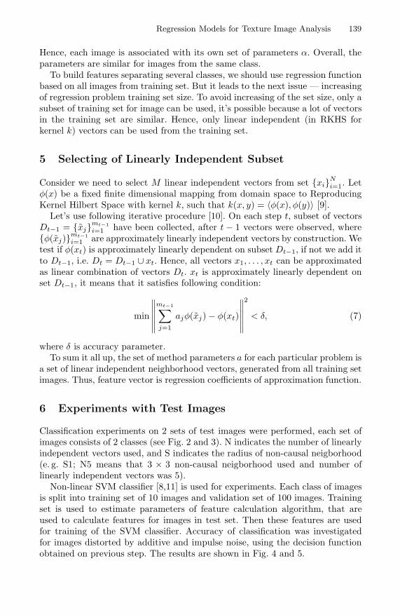
Regression Models for Texture Image Analysis 139
Hence, each image is associated with its own set of parameters α. Overall, theparameters are similar for images from the same class.
To build features separating several classes, we should use regression functionbased on all images from training set. But it leads to the next issue — increasingof regression problem training set size. To avoid increasing of the set size, only asubset of training set for image can be used, it’s possible because a lot of vectorsin the training set are similar. Hence, only linear independent (in RKHS forkernel k) vectors can be used from the training set.
5 Selecting of Linearly Independent Subset
Consider we need to select M linear independent vectors from set xiNi=1. Let
φ(x) be a fixed finite dimensional mapping from domain space to ReproducingKernel Hilbert Space with kernel k, such that k(x, y) = 〈φ(x), φ(y)〉 [9].
Let’s use following iterative procedure [10]. On each step t, subset of vectorsDt−1 = xjmt−1
i=1 have been collected, after t − 1 vectors were observed, whereφ(xj)mt−1
i=1 are approximately linearly independent vectors by construction. Wetest if φ(xt) is approximately linearly dependent on subset Dt−1, if not we add itto Dt−1, i.e. Dt = Dt−1 ∪ xt. Hence, all vectors x1, . . . , xt can be approximatedas linear combination of vectors Dt. xt is approximately linearly dependent onset Dt−1, it means that it satisfies following condition:
min
∥∥∥∥∥∥
mt−1∑
j=1
ajφ(xj) − φ(xt)
∥∥∥∥∥∥
2
< δ, (7)
where δ is accuracy parameter.To sum it all up, the set of method parameters a for each particular problem is
a set of linear independent neighborhood vectors, generated from all training setimages. Thus, feature vector is regression coefficients of approximation function.
6 Experiments with Test Images
Classification experiments on 2 sets of test images were performed, each set ofimages consists of 2 classes (see Fig. 2 and 3). N indicates the number of linearlyindependent vectors used, and S indicates the radius of non-causal neigborhood(e. g. S1; N5 means that 3 × 3 non-causal neigborhood used and number oflinearly independent vectors was 5).
Non-linear SVM classifier [8,11] is used for experiments. Each class of imagesis split into training set of 10 images and validation set of 100 images. Trainingset is used to estimate parameters of feature calculation algorithm, that areused to calculate features for images in test set. Then these features are usedfor training of the SVM classifier. Accuracy of classification was investigatedfor images distorted by additive and impulse noise, using the decision functionobtained on previous step. The results are shown in Fig. 4 and 5.
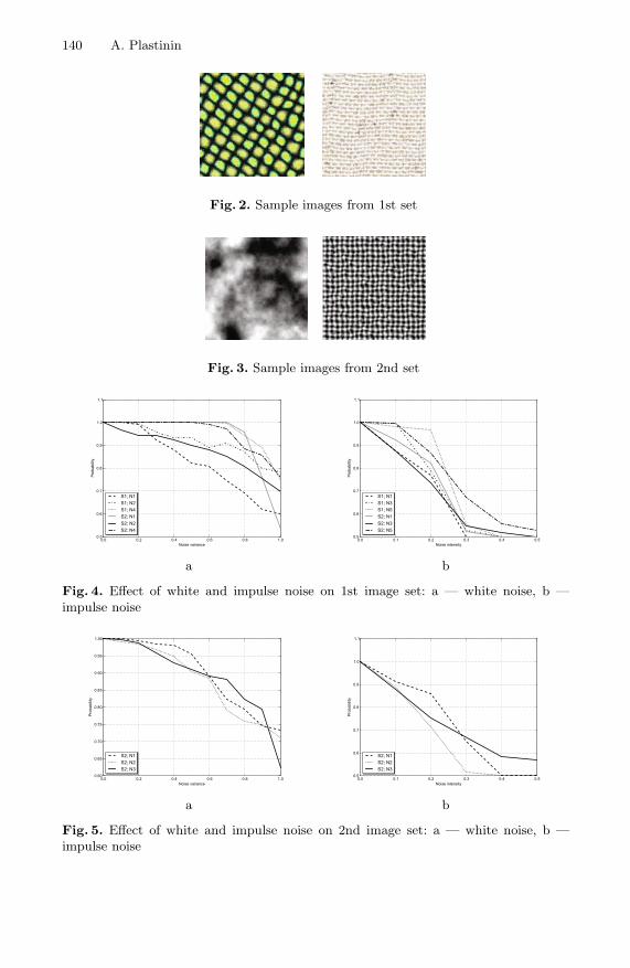
140 A. Plastinin
Fig. 2. Sample images from 1st set
Fig. 3. Sample images from 2nd set
Noise variance
Probability
S1; N1
S1; N2
S1; N4
S2; N1
S2; N2
S2; N4
a
Noise intensity
Probability
S1; N1
S1; N3
S1; N5
S2; N1
S2; N3
S2; N5
b
Fig. 4. Effect of white and impulse noise on 1st image set: a — white noise, b —impulse noise
Noise variance
Probability
S2; N1
S2; N2
S2; N3
a
Noise intensity
Probability
S2; N1
S2; N2
S2; N3
b
Fig. 5. Effect of white and impulse noise on 2nd image set: a — white noise, b —impulse noise
Regression Models for Texture Image Analysis 141
7 Conclusion
In our research work the general framework for estimating textural features,which utilizes domain specific information from training set, is described. Pro-posed method is used for formalization of features estimation algorithm based onapproximation of pixels dependency function, for images with markov randomfield model.
The method has following advantages: domain specific features increase classi-fication quality (in terms of correct classification probability); features are stableto additive and impulse noise.
References
1. Haralick, R.M.: Statistical and structural approaches to texture. Proceedings ofthe IEEE 67(5), 786–804 (1979)
2. Haralick, R.M., Shanmugam, K., Dinstein, I.: Textural Features for Image Classifi-cation. IEEE Transactions on Systems, Man, and Cybernetics SMC-3(6), 610–621(1973)
3. Tamura, H., Mori, S., Yamawaki, T.: Textural Features Corresponding to VisualPerception. IEEE Transaction on Systems, Man, and Cybernetcs SMC-8(6), 460–472 (1978)
4. Winkler, G.: Image Analysis, Random Fields and Dynamic Monte Carlo Methods,p. 324. Springer, Heidelberg (1995)
5. Paget, R.: Nonparametric Markov Random Field Models for Natural Textures Im-ages, Ph.D. thesis, University of Queensland, St Lucia, QLD Australia (December1999)
6. Kaulgud, N., Desai, U.B.: Efficient color image restoration using Markov randomfield. In: TENCON 1998. 1998 IEEE Region 10 International Conference on GlobalConnectivity in Energy, Computer, Communication and Control, vol. 1, pp. 41–44(1998)
7. Li, S.Z.: Markov Random Field Modeling in Image Analysis, 3rd edn. Springer,Heidelberg (2009)
8. Scholkopf, B., Smola, A.J.: Learning with Kernels Support Vector Machines, Reg-ularization, Optimization, and Beyond. MIT Press, Cambridge (2001)
9. Hastie, T., Tibshirani, R., Friedman, J.: The Elements of Statistical Learning. DataMining, Inference, and Prediction, 2nd edn. Springer, Heidelberg (2009)
10. Engel, Y., Mannor, S., Meir, R.: The Kernel Recursive Least-Squares Algorithm.IEEE Transactions on Signal Processing 52(8) (2004)
11. Vapnik, V.: Statistical Learning Theory. Wiley, Chichester (1998)

Shape Descriptor Based on the Volume of
Transformed Image Boundary
Xavier Descombes1 and Sergey Komech2
1 EPI Ariana, INRIA SAM, Sophia Antipolis, [email protected]
2 Dobrushin Lab., IITP, Moscow, [email protected]
Abstract. In this paper, we derive new shape descriptors based on adirectional characterization. The main idea is to study the behavior ofthe shape neighborhood under family of transformations. We obtain adescription invariant with respect to rotation, reflection, translation andscaling. We consider family of volume-preserving transformations. Ourdescriptor is based on the volume of the neighbourhood of transformedimage. A well-defined metric is then proposed on the associated featurespace. We show the continuity of this metric. Some results on shaperetrieval are provided on Kimia 216 and part of MPEG-7 CE-Shape-1databases to show the accuracy of the proposed shape metric.
1 Introduction
Shape characterization is becoming a crucial challenge in image analysis. Theincreasing resolution of new sensors, satellite images or scanners provides infor-mation on the object geometry which can be interpreted by shape analysis. Thesize of data basis also requires some efficient tools for analyzing shapes, for exam-ple in applications such as image retrieval. Reviews of proposed representationscan be found in [4,5]. One class of methods consists in defining shapes descrip-tors based on shape signatures histogram signatures, shape invariant moments,contrast, matrices or spectral features. A shape representation is evaluated withrespect to its robustness, w.r.t. noise and/or intra-class variability, compactionof the description, its invariance properties and its efficiency in terms of com-putation time. According to Zhang and Lu [5], the different approaches can beclassified into contour-based and region-based methods, and within each classbetween structural and global approaches. In this paper we consider shapes asbinary silhouette of objects and concentrate on global approaches. Simple globalshape descriptors embed area, orientation, convexity, bending energy [6,7]. Usu-ally, these descriptors are not sufficiently sensitive to details to provide goodscores in image retrieval. Distances between shapes or surfaces have been pro-posed, such as the Hausdorf distance or some modification to reduce sensitivityto outlier [8,9]. In this setting, the invariance properties can be obtained by tak-ing the minimum distance over the corresponding group of transformation. Akey issue is to consider a metric for which the minimum is computed with a lowcomputational complexity.
S.O. Kuznetsov et al. (Eds.): PReMI 2011, LNCS 6744, pp. 142–147, 2011.c© Springer-Verlag Berlin Heidelberg 2011

Shape Descriptor Based on the Volume 143
In this paper, we derive a 2D signature of shapes and propose a metric on theassociated feature space. The first idea consists of a description of the bound-ary regularity by comparing the volume of the boundary neighborhood with theshape volume. The second idea is to study the behavior of this descriptor undershape transformations. We thus define a family of diffeomorphisms consisting inexpanding the shape in one direction and contracting it in the orthogonal direc-tion. In that way, for a given detail, there exists at least such a transformationenlarging its contribution to the descriptor and another one reducing it. We thenderive a well defined metric on the feature space, and show its performance forshape discrimination on databases of various size.
We describe the proposed shape space and define a metric on it in Section 2. Adiscretization of the metric is described and evaluated on two different databasesin Section 3. Finally, conclusion and perspectives are drawn in Section 4.
2 A Topological Description of Shapes
2.1 Shape Space
We consider shapes as 2D silhouettes of bounded objects in the image plane.
Definition 1. The pre-shape space S is the set of subsets of IR2 satisfying thefollowing conditions:
1. ∀a ∈ S, a is compact and connected, with a strictly positive area,2. ∀a ∈ S, IR2 \ a is connected (a has no hole).
Let us consider a shape a ∈ S. Define the closed ε-neighborhood of the set ain the sense of the Euclidean metric as Oε(a) = x ∈ IR2 : e(x, a) ≤ ε, ε ≥ 0,where e(·, ·) is the Euclidean distance.
On this pre-shape space, we consider the Hausdorff metric (which is well-defined, see, for example, [2]) for the sets in IR2:
ρ(a, b) = infδ > 0 : a ⊂ Oδ(b), b ⊂ Oδ(a),where a, b ⊂ S.
A shape space should embed some invariance properties. Let G be the groupof transformations of IR2 generated by rotations, translations, reflections andscaling : G = SL±
2 (IR) × IR+. To define a shape space S isometry- and scale-invariant, we consider:
S = S/G . (1)
For a given A ∈ S, we note r(A) = a ∈ S : vol(a) = 1, G(a) = A, where vol(·)is the area of the set.
Therefore, on the shape space S, the Hausdorff metric becomes:
d(A, B) = infρ(a, b) | a ∈ r(A), b ∈ r(B), (2)
where A, B ∈ S (note that this metric can be compared with the Procrustesdistance for sets consisting of finite number of points [3,1]). The proof of thefollowing proposition is not very hard and we will omit it due to the space limit.

144 X. Descombes and S. Komech
Proposition 1. d(·, ·) is a well-defined metric on S.
2.2 Volume Descriptor and Family of Transformations
The main idea of the proposed description is to characterize the behavior ofshapes under some transformations. These transformations aim at enlightingsmall characteristic details. We first consider the volume behavior under somedilation. Intuitively, this volume will increase more for sinuous shape boundariesthan for smooth shapes. Let us consider a shape a ∈ S. Idea of our shapedescriptor is based on analyzing the fraction
P ε(a) =vol(Oε(a) \ a)
vol(a), (3)
where vol(·) is the area of the set. This parameter is well-defined (vol(a) = 0).We consider a family F(θ,β) of linear transformations of IR2 in order to ob-
tain more significant information about shapes. The goal of such transformationsis to emphasize ”features” of the shape in specific direction. These transforma-tions are defined as follows:
F(θ,β) :=
(β cos2 θ + 1
βsin2 θ (β − 1
β) sin θ cos θ
(β − 1β) sin θ cos θ β sin2 θ + 1
βcos2 θ
), (4)
where θ ∈ [−π2, π
2], β ≥ 1. Every F(θ,β) is β-times expanding in one direction
(with angle θ) and β-times contracting in orthogonal, so it is a volume-preservingtransformation.
For every set a ⊂ IR2, we obtain the map
a → P ε(θ,β)(a) :=
vol(Oε(F(θ,β)a) \ F(θ,β)a)vol(a)
, θ ∈ [−π
2,π
2], β ≥ 1, ε > 0 . (5)
It is clear that P ε(θ,β)(a) is a continuous function of ε, θ and β and P ε
(−π2 ,β)(a) =
P ε( π
2 ,β)(a). Note, that this function is a constant, if a is a ball (ε, β are fixed).Let Rγ be the rotation by an angle γ. We have the following property:
Property 1. ∀θ ∈ [−π2 , π
2 ], P ε(θ,β)(Rγa) = P ε
((θ+ π2 +γ)mod(π)−π
2 ,β)(a).
We consider Rx, the reflection with respect to x axis (horizontal line). Wehave the following property:
Property 2. ∀θ ∈ [−π2 , π
2 ], P ε(θ,β)(Rxa) = P ε
(−θ,β)(a).
Let us denote R the group of transformations generated by Properties 1 and2. The shape representation space R we consider for the fixed ε > 0 is thendefined by the following mapping:
Φ : S → R = C0([−π
2,π
2] × [1,∞])/R,
A → P ε(θ,β)(a)/R, a ∈ r(A), A ∈ S. (6)

Shape Descriptor Based on the Volume 145
20 40 60 80 100 120
10
20
30
40
50
60
70
80
90
22.5
33.5
44.5
5
−100
−50
0
50
1000.4
0.5
0.6
0.7
0.8
0.9
1
1.1
1.2
1.3
50 100 150 200
20
40
60
80
100
120
140
160
180
50 100 150 200
20
40
60
80
100
120
140
160
180
50 100 150 200
20
40
60
80
100
120
140
160
180
50 100 150 200
20
40
60
80
100
120
140
160
180
Fig. 1. Calf (top left) and the associated representation Pn(F(γ,β)). The bottom linerepresents F(γ,β) for β = 2 and γ = 45, 90,−45, 0 (the shape is in black and theneighborhood in grey).
On Figure 1, we can remark that the function Pn(γ,β)(a) increases more in two
directions, corresponding to an extention of both the calf body and its legs.We consider situation with no information about foreshortening and all rota-
tions are equally likely to occur. Finally, we consider the following metric on R:
l(Φ(A), Φ(B)) := infa,b
⎛
⎜⎝∫
[−π2 , π
2 ]×[1,∞]
(P ε(θ,β)(a) − P ε
(θ,β)(b))2 e−κβdβ dθ
⎞
⎟⎠
1/2
, (7)
where κ > 0 is a parameter, a ∈ r(A), b ∈ r(B). The integral on the right-handside converges due to P ε
(θ,β)(a) is almost linear function of β for β big enough.We thus have defined a map between the shape space and the feature space.
Two similar shapes should be associated to close points in the feature space.This property can be established by the continuity of mapping Φ with respect tothe metrics defined in both spaces. The proof of the following theorem we willomit.
Theorem 1. Φ : (S, d(, )) → (R, l(, )) is a continuous map.
3 Implementation and Results
3.1 Discretization
In practice, to compute the distance between two shapes, we have to discretizeequation (7). When analysing the surfaces representing the function Pn(F(θ,β)a)

146 X. Descombes and S. Komech
on Figure 1 it is clear that the embeded information is redundant. Indeed, thesurfaces are very smooth, so that we can employ a drastic discretization scheme,without loosing information. We consider n = 5 pixels neighbourhood.
Before computing the proposed feature, we normalize the shapes to V = 4000pixels (area) in order to satisfy the scale invariance.
3.2 MPEG-7 CE Shape-1 Part-B Data Set
We first evaluate the proposed approach for the 7 classes of well-known MPEG-7CE Shape-1 Part-B data set (70 classes, each class containing 20 similar objects).Although the classes are quite distinct, this data set contains important within-class variations (see [11]).
We consider four directions, θ ∈ −π4, 0, π
4, π, and two expanding coefficients
β ∈ 3, 5. The coefficient defined the metric is κ = 15.
We consider the proposed metric between each pair of shapes (except itself ofcourse, cause distance is 0) and report in Table 1 the percentage of correct nth
neighbors for each class. The total correct answers correspond to 98% for thefirst neighbors. If we consider the tenth neighbors, we still obtain a total scoreof 85% of good retrieval. This shows the robustness of the proposed metric.
Table 1. Retrieval scores on the 7 classes of MPEG-7 database
1st 2nd 3rd 4th 5th 6th 7th 8th 9th 10th
Bonefull 95 70 85 85 90 85 85 85 70 75
Heart 100 100 100 100 100 100 95 95 95 100
Glas 100 100 100 100 100 100 100 90 100 95
Fountain 100 100 100 100 100 100 100 100 100 100
Key 100 100 95 100 95 95 90 90 95 95
Fork 95 90 65 70 65 75 65 75 70 60
Hammerfull 95 95 80 30 30 35 30 40 35 15
3.3 Kimia Database
We considered the extended database defined by Kimia. It consists of 216 shapesdivided into 18 classes (see [11]). We consider θ∈90, 65, 45, 30, 0,−30,−45,−65,and two expanding coefficients β ∈ 3, 5. The global retrieval score is 91.2% forthe first neighbour, 80.1% for the second neighbour, 74.5% for the third neigh-bour, 72.7% for the fourth neighbour and 63% for the fifth neighbour. It showsthe robustness of the proposed metric in case of a rather big database.
Our results for the first neighbour 91.2% (as well as 98% for the first database)are comparable with 98% for SC-method and 100% stated recently in [10] forKimia 216 database. We besides have good result 80.6% for Bullseye score. Itshows good localization of different classes in feature space. Our descriptor isvery clear and transparent in implementation. It takes about 0.23 sec in Mat-Lab(Pentium 4, 2Gb) to find the first neighbour for one image among 215 others.

Shape Descriptor Based on the Volume 147
4 Conclusion
We have proposed a new metric on a shape space based on the shape propertiesafter applying family of diffeomorphisms. The proposed metric is well-definedand continuous. Retrieval results on two databases, one of them consisting of216 shapes, divided in 18 classes, have proven the relevance of this metric. Ourimage descriptor is invariant with respect to rotation, reflection, translation andscaling. We are currently studying the surjectivity of the associated mapping.We conjecture that surjectivity holds, at least for star shapes. Further studies (inparticular 3-D shape retrieval) also include the definition of a shape classificationalgorithm, based on this description.
References
1. Dryden, I.L., Mardia, K.V.: Statistical shape analysis. Wiley, New York (1998)2. Serra, J.: Image Analysis and Mathematical Morphology. Academic Press, New
York (1982)3. Kendall, D.G.: Shape Manifolds, Procrustean Metrics, and Complex Projective
Spaces. Bulletin of the London Mathematical Society 16, 81–121 (1984)4. Loncaric, S.: A survey of shape analysis techniques, J. Pattern Recognition 31(8),
983–1001 (1998)5. Zhang, D., Lu, G.: Reveiw of shape representation and description techniques. J.
Pattern Recognition 37, 1–19 (2004)6. Yong, I., Walker, J., Bowie, J.: An anlysis technique for biological shape. J. Com-
put. Graphics Image Process 25, 357–370 (1974)7. Peura, M., Livirinen, J.: Efficiency of simple shape descriptors. In: Third Interna-
tional Workshop on Visual Form, Capri, Italy, May 1997, pp. 443–451 (1997)8. Rucklidge, W.J.: Efficient locating objects using Hausdorff distance. Int. J. Com-
put. Vision 24(3), 251–270 (1997)9. Belongie, S., Malik, J., Puzicha, J.: Matching shapes. In: IEEE Eighth Int. Conf.
on Comput. Vision, Vancouver, Canada, July 2001, vol. I, pp. 454–461 (2001)10. Bai, X., Latecki, L.J.: Path Similarity Skeleton Graph Matching. IEEE Trans Pat-
tern Anal Mach Intell 30(7), 1282–1292 (2008)11. Sebastian, T., Klein, P., Kimia, B.: Recognition of shapes by editing their shock
graphs. IEEE Trans. Pattern Analysis and machine intelligence 25(5), 116–125(2004)

Color Image Segmentation Using a
Semi-wrapped Gaussian Mixture Model
Anandarup Roy1, Swapan K. Parui1, Debyani Nandi2, and Utpal Roy3
1 CVPR Unit, Indian Statistical Institute, Kolkata- 700108, [email protected], [email protected]
2 School of Education Tech., Jadavpur University, Kolkata- 700032, [email protected]
3 Dept. of Computer & System Sciences,Visva-Bharati University, Santiniketan- 731235, India
Abstract. This article deals with color image segmentation in the hue-saturation-value space. Hue, saturation and value components are sam-ples on a cylinder. A model for such data is provided by the semi-wrappedGaussian distribution. Further its mixture is used to approximate thehue-saturation-value distribution. The mixture parameters are estimatedusing the standard EM algorithm. The results are obtained on Berkeleysegmentation dataset. Comparisons are made with vM-Gauss mixturemodel, GMM and Mean-Shift procedures. Experimental results revealimprovement in segmentation by our method.
1 Introduction
Color image segmentation is becoming important in many applications sincecolor images are now easily available and can provide more information thangray level images. A popular way to represent a color image is the RGB system.However, due to its redundancy, many applications prefer the hue-saturation-value (HSV) color system. Consequently, segmentation in HSV space becomescrucial. In this article, we apply clustering based segmentation approach. The ba-sic idea is to directly cluster the pixels in a certain color space by employing someclustering algorithms. Such algorithms include Mean-Shift and normalized-cutprocedures [1] which are used widely. Segmenting an image into clusters involvesdetermining which clusters generate the image pixels, which is the hidden infor-mation. Under this consideration, a mixture model based approach can be used.This approach assumes a mixture distribution approximating the distribution ofimage pixels. The mixture parameters can be estimated using expectation maxi-mization algorithm. Such an earlier attempt was made by Carson et. al. [2] usingGaussian Mixture Model (GMM). Later, Bougulia et. al. [3] considered the as-pect of skewness of color bands and applied a mixture of Dirichlet distributionsfor the joint distribution of RGB color spectrum.
The HSV system is a mixture of angular (hue) and linear (saturation, value)data. Mere linear mixture models may fail to model the hue distribution. Hue
S.O. Kuznetsov et al. (Eds.): PReMI 2011, LNCS 6744, pp. 148–153, 2011.c© Springer-Verlag Berlin Heidelberg 2011
Color Image Segmentation Using a Semi-wrapped Gaussian Mixture Model 149
can be represented by a random variable Θ ∈ [0, 2π). A direct modeling ofΘ can be avoided by transforming it into its linear representation (cos θ, sin θ)and applying a linear mixture model. However the pair (cos θ, sin θ) may behighly correlated, thus may pose the problem of singularity of the covariancematrix for some mixture components. Instead, we use the wrapped Gaussiandistribution [4] for Θ. This distribution is a wrapping of linear Gaussian distri-bution around a circle. To cope with the circular-linear characteristics we needto wrap only one variable (corresponding to Θ) of a multivariate Gaussian dis-tribution, whereas the other unwrapped variables represent linear portion. Thisdistribution is termed as semi-wrapped Gaussian distribution [5]. Its mixture isused to approximate the HSV joint data distribution. An alternative model inhue-saturation (HS) space was suggested by Roy et. al. [6] using a mixture ofvM-Gauss distribution. However, joint distribution in HSV space has not beenproposed yet. An EM algorithm is designed to estimate the mixture parameters.The Berkeley segmentation Dataset [7] is used to test the performance of themethods. We compare our segmentation with vM-Gauss mixture model, GMMand Mean-Shift algorithms using probabilistic rand index.
2 Semi-wrapped Gaussian Distributions: Description andMixture
Our aim is to devise a mixture of multivariate Gaussian distributions havingboth circular and linear variables. In this context, the wrapped Gaussian isa suitable choice. Otherwise, the von Mises distribution can replace wrappedGaussian. However, forming a joint distribution using von Mises is difficult. Thus,in spite of the practical drawbacks in the parameter estimation, the wrappedGaussian distribution, is chosen. The remaining part of this section presents abrief overview on semi-wrapped Gaussian distribution, and its mixture.
2.1 Wrapped Gaussian Distribution
In particular, for Nμ,σ(x) being a univariate Gaussian distribution the wrappedunivariate Gaussian distribution is defined as follows.
Nwμc,σc(υ) =
∑
w∈Z
Nμ,σ(υ + 2wπ) (1)
where υ ∈ [0, 2π). Nwμc,σc(υ) is unimodal and symmetric about μc. It can be
shown that the circular mean and variance (μc, σc) are related to linear meanand variance (μ, σ) by the equations μc = μ(mod 2π) and σ2 = −2 log(1 − σc).In a similar way the multivariate Gaussian distribution can be wrapped onto asphere to obtain the wrapped version.
2.2 Semi-wrapped Gaussian Distribution and Mixture
Let us consider an HSV image. Then, the hue component is angular, whereas sat-uration and value components are linear. For such situations, a suitable modeling

150 A. Roy et al.
should employ a distribution that is wrapped in the angular and non-wrappedin the linear dimensions. The semi-wrapped Gaussian distribution [5] serves thispurpose well enough. For simplicity we assume only the first variable (Θ) isangular (this really is for our problem) and others (x) linear. With these specifi-cations the semi-wrapped Gaussian distribution can be formed by wrapping thefirst variable of a multivariate Gaussian distribution. Its density is given by:
N swμc,Σc(θ,x) =
∑
w∈Z
Nμ,Σ(θ + 2wπ,x), (2)
with mean μc and covariance matrix Σc.Let us now define the mixture model of K semi-wrapped Gaussian distribu-
tions (SWGMM). The density of the mixture is given by:
f(θ,x|Ξ) =K∑
h=1
P (h)N swΞh
(θ,x). (3)
where P (h)(0 ≤ P (h) ≤ 1 andK∑
h=1
P (h) = 1) are the mixing proportions,
N swΞh
(θ,x) is the semi-wrapped Gaussian distribution representing the hth com-
ponent of the mixture and Ξh is the set of parameters of the hth component. Thesymbol Ξ = (Ξ1, . . . , ΞK , P (1), . . . , P (K)) refers to the entire set of parametersto be estimated.
3 Maximum Likelihood Estimation
Let ℵ = p1, . . . , pN be a finite set of N samples drawn independently from theSWGMM. Here pi = (θi,xi) is a circular-linear data. To maximize the likeli-hood function, the expectation maximization (EM) is widely used. The clusterinformation and wrapping are the hidden variables. The standard EM settingsexpress the distribution of hidden variables by:
q(h, w|pi) =P (h)Nμ
h,Σh
(pi + 2wπ)K∑
l=1
P (l)N swΞ l
(pi). (4)
Here pi+2wπ indicates the tuple (θ+2wπ,x). The EM algorithm maximizes thelog-likelihood modified by the inclusion of q(h, w|pi). To maximize the modifiedlog-likelihood we may go independently for a priory probabilities P (h) and theparameters Ξh. The a priori probabilities can be found out with:
P (h) =1N
N∑
i=1
∑
w∈Z
q(h, w|pi). (5)

Color Image Segmentation Using a Semi-wrapped Gaussian Mixture Model 151
The expressions for μch and Σc
h are quite similar to the linear Gaussian mixtureand obtained using:
μch =
N∑i=1
∑w∈Z
q(h, w|pi)(pi + 2wπ)
N∑i=1
∑w∈Z
q(h, w|pi)(6)
Σch =
N∑i=1
∑w∈Z
q(h, w|pi)(pi + 2wπ − μch)(pi + 2wπ − μc
h)T
N∑i=1
∑w∈Z
q(h, w|pi). (7)
In practice w hold values −1, 0 and 1. We continue writing w ∈ Z for complete-ness.
4 Color Image Segmentation
Let us assume that the hue, saturation and value components of an HSV imagearise from a SWGMM (Eq. 3). The EM method estimates mixture parametersby iterating expectation (Eq. 4) and maximization steps (Eqs. 5, 6 and 7). Thesesteps iterate until the log-likelihood stabilizes. We apply K-Means algorithm onHSV image to obtain initial clustering. Initially, μc
h and Σch are estimated as
follows.
μch =
Nh∑i=1
∑w∈Z
(pi + 2wπ)
Nhand Σc
h =
Nh∑i=1
∑w∈Z
(pi + 2wπ − μch)(pi + 2wπ − μc
h)T
Nh.
(8)The a priori probabilities are set with P (h) = Nh
N where Nh is the number ofelements in hth cluster. In order to detect the number of clusters automaticallywe use the Schwarz’s Bayesian Information Criterion (BIC). Optimum valueof K is the first local minimum of BIC. Note, for the gray portions, the huebecomes undefined. We separate out the gray portions before employing EM.A separate clustering should be employed with the gray portions. Yet, here weencounter only a few gray pixels mostly in the background and thus leave themto minimize time complexity.
5 Evaluation of Segmentation
To evaluate the quality of segmentation algorithm we have to compare the result-ing clusters with the ground-truth segmentations. A good survey on evaluationmethodologies can be found in [8]. Recently, Unnikrishnan et. al. [9] proposed aProbabilistic Rand Index (PRI) which is a generalization of classical Rand Index.The PRI is further applied to evaluate a color segmentation procedure designed

152 A. Roy et al.
(a)
(b)
(c)
Fig. 1. (a) Example images of Berkeley segmentation dataset. Image Ids are (fromtop left to right) “24063”, “100075”, “112082” and “376020”. (b)(c) Correspondingsegmentations in HS and HSV space respectively.
by Ilea and Whelan [10]. The PRI allows comparison of a test segmentation withmultiple ground-truth images by evaluating the pairwise relationships betweenpixels. It takes values in the range [0, 1], where a higher PRI value indicates abetter match between the segmented result and the ground-truth data. In thisstudy we use PRI to evaluate the segmentation process.
6 Results and Discussions
The Berkeley segmentation dataset [7] contains several color images of naturalscenes. The images contain at least one distinguishable and identifiable objectembedded in a natural scene. The images we consider have ground-truth in theform of manual segmentation performed by several users independently. Let usnow present some results after running the algorithm in HS (Fig. 1(b)) andHSV (Fig. 1(c)) space. Visually it is difficult to assess which segmentation isbetter. This can be done using the PRI. We compare SWGMM with the mix-ture model of vM-Gauss distribution (vMGMM), the GMM and the Mean-Shiftprocedures (last two in RGB). The comparison results are presented in Fig. 2.The Mean-Shift performs better for a few images. The GMM, on the other hand,outperforms Mean-Shift in most cases. The vMGMM assumes independence ofhue and saturation. By noting that SWGMM outperforms vMGMM, we couldconclude, the correlation present in hue, saturation and/or value should be cru-cial for segmentation. The SWGMM in HSV space can show better performancefor some image than GMM and Mean-Shift. A detailed statistical study mayreveal the significance of the results. We are in a process to design that.

Color Image Segmentation Using a Semi-wrapped Gaussian Mixture Model 153
24063 100075 112082 376020 113044 153077 296059 940790.6
0.65
0.7
0.75
0.8
0.85
0.9
Image Id
PR
I val
ues
SWGMM−HSvMGauss−HSSWGMM−HSVGMM−RGBMean−Shift−RGB
Fig. 2. Comparison of different segmentation algorithms with respect to PRI
7 Summery and Future Scope
We study the problem of color image segmentation in HSV space. A mixture ofsemi-wrapped Gaussian distributions is used to model hue, saturation and valuedata. Results and comparisons are on Berkeley segmentation dataset. Futurework may include the study of different forms of joint distributions on circular-linear data.
References
1. Tao, W., Jin, H., Zhang, Y.: Color image segmentation based on mean shift andnormalized cuts. IEEE Trans. on SMC(B) 37, 1382–1389 (2007)
2. Carson, C., Belongie, S., Greenspan, H., Malik, J.: Blobworld: Image segmenta-tion using expectation-maximization and its application to image querying. IEEETrans. on PAMI 24, 1026–1038 (2002)
3. Bougulia, N., Ziou, D., Vaillancourt, J.: Unsupervised learning of a finite mixturemodel based on the dirichlet distribution and its application. IEEE Trans. on ImageProcessing 13, 1533–1543 (2004)
4. Mardia, K.V., Jupp, P.: Directional Statistics. John Wiley and Sons Ltd., Chich-ester (2000)
5. Bahlmann, C.: Directional features in online handwriting recognition. PatternRecognition 39, 115–125 (2006)
6. Roy, A., Parui, S.K., Roy, U.: A color based image segmentation and its applicationto text segmentation. In: Proc. of Indian Conf. on Computer Vision, Graphics andImage Processing, pp. 313–319 (2008)
7. Martin, D., Fowlkes, C., Tal, D., Malik, J.: A database of human segmented naturalimages and its application to evaluating segmentation algorithms and measuringecological statistics. In: Proc. Int Conf. Computer Vision, pp. 416–423 (2001)
8. Chabrier, S., Laurent, H., Rosenburger, C., Marche, P.: A comparative study ofsupervised evaluation criteria for image segmentation. In: Proc. of the EuropeanSignal Processing Conference, pp. 1143–1146 (2004)
9. Unnikrishnan, R., Pantofaru, C., Hebert, M.: Toward objective evaluation of imagesegmentation algorithms. IEEE Trans. on PAMI 29, 929–944 (2007)
10. Ilea, D.E., Whelan, P.F.: Ctex—an adaptive unsupervised segmentation algorithmbased on color-texture coherence. IEEE Trans. on Image Processing 17, 1926–1939(2008)
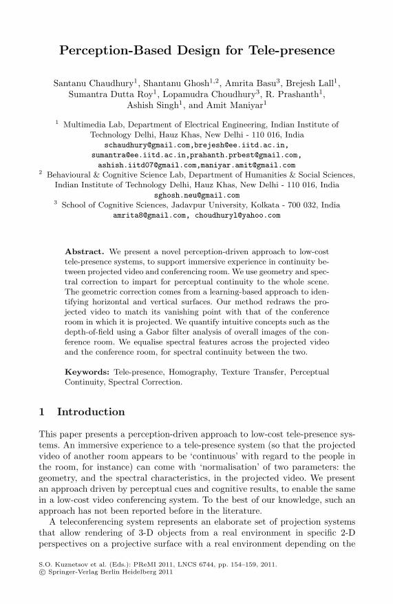
Perception-Based Design for Tele-presence
Santanu Chaudhury1, Shantanu Ghosh1,2, Amrita Basu3, Brejesh Lall1,Sumantra Dutta Roy1, Lopamudra Choudhury3, R. Prashanth1,
Ashish Singh1, and Amit Maniyar1
1 Multimedia Lab, Department of Electrical Engineering, Indian Institute ofTechnology Delhi, Hauz Khas, New Delhi - 110 016, India
[email protected],[email protected],
[email protected],[email protected],
[email protected],[email protected] Behavioural & Cognitive Science Lab, Department of Humanities & Social Sciences,
Indian Institute of Technology Delhi, Hauz Khas, New Delhi - 110 016, [email protected]
3 School of Cognitive Sciences, Jadavpur University, Kolkata - 700 032, [email protected], [email protected]
Abstract. We present a novel perception-driven approach to low-costtele-presence systems, to support immersive experience in continuity be-tween projected video and conferencing room. We use geometry and spec-tral correction to impart for perceptual continuity to the whole scene.The geometric correction comes from a learning-based approach to iden-tifying horizontal and vertical surfaces. Our method redraws the pro-jected video to match its vanishing point with that of the conferenceroom in which it is projected. We quantify intuitive concepts such as thedepth-of-field using a Gabor filter analysis of overall images of the con-ference room. We equalise spectral features across the projected videoand the conference room, for spectral continuity between the two.
Keywords: Tele-presence, Homography, Texture Transfer, PerceptualContinuity, Spectral Correction.
1 Introduction
This paper presents a perception-driven approach to low-cost tele-presence sys-tems. An immersive experience to a tele-presence system (so that the projectedvideo of another room appears to be ‘continuous’ with regard to the people inthe room, for instance) can come with ‘normalisation’ of two parameters: thegeometry, and the spectral characteristics, in the projected video. We presentan approach driven by perceptual cues and cognitive results, to enable the samein a low-cost video conferencing system. To the best of our knowledge, such anapproach has not been reported before in the literature.
A teleconferencing system represents an elaborate set of projection systemsthat allow rendering of 3-D objects from a real environment in specific 2-Dperspectives on a projective surface with a real environment depending on the
S.O. Kuznetsov et al. (Eds.): PReMI 2011, LNCS 6744, pp. 154–159, 2011.c© Springer-Verlag Berlin Heidelberg 2011

Perception-Based Design for Tele-presence 155
projection angle of the camera. Such a technologically mediated communicationinvolves certain degree of ‘presence’ or a ‘feeling of being there’ that allows theconferees to respond realistically to events and situations in the projected toreal environment. Perception of such extensions may occur due to geometricalalignments, rendering of objects, and illumination patterns between real andprojected environments. The present ‘state of the art’ teleconferencing systemsutilize very high-end studios congruent in geometrical alignments and illumi-nation patterns to enhance this ‘same-room effect’. However, providing exactlysimilar environments for the virtual and the real counterparts is often difficult toachieve and may not provide a ‘seamless’ integration of the real and the virtualenvironments. There are obvious constraints associated with such a system, likesmall size and relative independence of location of the projection screen thatdrives the need for designing a cognitive cue-based geometrical and spectral cor-rection algorithm for an ‘immersive’ experience during conferences. Hence wefavour a scene recognition approach to the problem over the current reconstruc-tion techniques and introduce an algorithm that leads to an enhanced visualcontinuity. This is achieved by extracting semantic category information andvisual congruence.
In this paper, we present the results of a computational approach basedon classification and organisation of tele-presence video conferencing framesinto congruent and non-congruent domains with respect to projected-to-realsymmetry-based continuity and depth perception of the two scenes. We utiliselower level information such as textures and perceptual feedback to build up aconfidence contour of the context and compute the perceptual difference betweenthe two contexts. Further, our method minimizes the perceptual difference byadjusting the intermediate level properties used for identification of contexts.The perceptual cue used is the continuity of vanishing lines from the projectedimages, matching the vanishing lines in an image of the conference room. Ourmethod scores on three points: determination of the spectral match betweenreal-to-projected environments, a continuous organisation between the real andthe projected environments and determination of a geometric alignment matchbetween the projected and real scenes.
2 Tele-presence and Video Conferencing
A scene may be described with reference to the observer who has a ‘fixated pointof view’ in an image. Oliva and Torralba [5] propose to consider the absolutedistance between the observer and the fixated zone as a principal property todefine a ‘scene’. A ‘view on a scene’ begins when there is actually a larger spacebetween the observer and the fixated point, usually after 5 meters (typically itrefers to a single image in image processing/computational vision). In a videoconferencing situation however, an ambiguity in the perception of the fixatedpoint is created by introducing a projected image (thereby creating at leasta two scene system). Perception of a video conferencing scene may thereforebe defined as a composite of two scenes where the fixation point is altered by

156 S. Chaudhury et al.
an introduction of a projected scene. We seek to create a ‘unified’ scene intwo different ways. First, we try to align the geometry of the two scenes in acomputationally simple method (Section 3). Next, we seek to unify the spectralcharacteristics of the projected video, and a conference room, using low-levelfeatures which are descriptors of a higher level percept (Section 4). This createsa visual illusion of the same room in such a composite scene by describing featurecomposites to yield higher level features. The human visual system uses this forfast and efficient detection of scene congruence between the projected and realenvironments.
3 Geometric Correction: Novel View Generation
The first step in our approach is to correct for the geometry of the projected videoscene, so that it appears to be perceptually ‘continuous’ with the geometry ofthe room in which the video is projected. There is a wealth of literature on novelview generation, given either a number of views, or a single one. (Representativereferences for the two are [2] and [1], respectively). For multiple views, for aslowly moving camera, one can establish correspondences between different viewsof the same scene (using any tracker, for instance). A typical approach firstcomputes the projective structure, and using further constraints, updates it toaffine, metric or Euclidean, depending on the nature of the constraints. For thesingle view method, again one needs specific constraints [1]. These methods arecomputationally complex, and often quite cumbersome.
We adopt a different methodology - one based on the ideas of Hoiem, Efrosand Hebert [3]. This is a fully automatic method for creating a 3-D model froma single photograph. We use their basic idea of trying to statistically modelgeometric classes defined by their orientations, rather than trying to recoverthe precise geometry. In our case, we learn labels corresponding to coarse cat-egories ‘horizontal’, ‘vertical’, and ‘background’ from representative images ofvideo conferencing scenes. Based on the statistical learning of the labels, givena new video conferencing scene, the algorithm segments image regions, groupsthem together, and then uses the learnt information into the three categories,and then attempts to recreate the structure of the scene for the three categories.Given the estimated structure for the horizontal and vertical segments for in-stance, we specify sample camera parameters for the new viewpoint. The newviewpoint is estimated according to the orientation of the lines in an image ofthe video conferencing environment. We adopt a Hough transform-like approach,and vote on the different possible vanishing points (otherwise known as the FoE:‘focus of expansion’) within the image of the video conferencing room in ques-tion. We assume that the one getting the highest vote is the required point,and we orient the camera parameters in order to project the above estimatedstructure on the projection screen in the video conferencing room, in order toequalise the two vanishing points. This is the essence of trying to ‘equalise’ thetwo viewing geometries. Fig. 1 shows two examples of using such an automaticcorrection for the projected frames. In the first one, the desired image has the
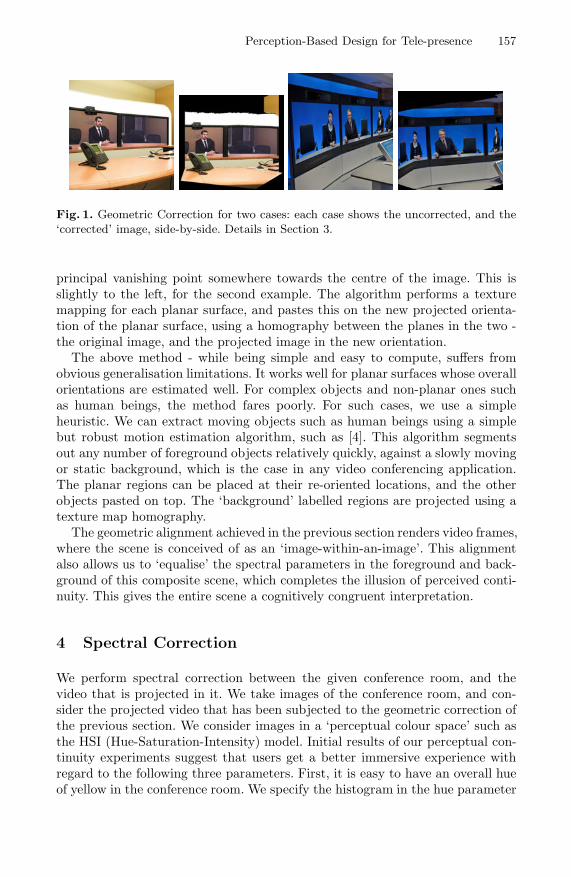
Perception-Based Design for Tele-presence 157
Fig. 1. Geometric Correction for two cases: each case shows the uncorrected, and the‘corrected’ image, side-by-side. Details in Section 3.
principal vanishing point somewhere towards the centre of the image. This isslightly to the left, for the second example. The algorithm performs a texturemapping for each planar surface, and pastes this on the new projected orienta-tion of the planar surface, using a homography between the planes in the two -the original image, and the projected image in the new orientation.
The above method - while being simple and easy to compute, suffers fromobvious generalisation limitations. It works well for planar surfaces whose overallorientations are estimated well. For complex objects and non-planar ones suchas human beings, the method fares poorly. For such cases, we use a simpleheuristic. We can extract moving objects such as human beings using a simplebut robust motion estimation algorithm, such as [4]. This algorithm segmentsout any number of foreground objects relatively quickly, against a slowly movingor static background, which is the case in any video conferencing application.The planar regions can be placed at their re-oriented locations, and the otherobjects pasted on top. The ‘background’ labelled regions are projected using atexture map homography.
The geometric alignment achieved in the previous section renders video frames,where the scene is conceived of as an ‘image-within-an-image’. This alignmentalso allows us to ‘equalise’ the spectral parameters in the foreground and back-ground of this composite scene, which completes the illusion of perceived conti-nuity. This gives the entire scene a cognitively congruent interpretation.
4 Spectral Correction
We perform spectral correction between the given conference room, and thevideo that is projected in it. We take images of the conference room, and con-sider the projected video that has been subjected to the geometric correction ofthe previous section. We consider images in a ‘perceptual colour space’ such asthe HSI (Hue-Saturation-Intensity) model. Initial results of our perceptual con-tinuity experiments suggest that users get a better immersive experience withregard to the following three parameters. First, it is easy to have an overall hueof yellow in the conference room. We specify the histogram in the hue parameter

158 S. Chaudhury et al.
in the projected video, to peak around yellow. Next, we perform a histogramequalisation on the saturation and intensity components.
We described the organisation of the projected-to-real tele-presence scenesalong two semantic axes providing an ideal Spectral and Geometric MatchingTemplate (SGMT) (i.e., from general indoor scenes to specific video conferencingscenes; from highly textured ‘indoor’-scapes to no textures, from ‘deep’ rooms to‘shallow’ rooms and from ‘artificial’ to ‘natural’ indoor scenes with respect to analignment of vanishing lines). All images were pre-processed to reduce the effectsof large shadows that may hide important parts of the scene and to minimizethe impact of high contrasted objects which would disturb the power spectrumshape of the background image. First, we apply a logarithmic function to theintensity distribution. Then we attenuate the very low spatial frequencies byapplying a high pass filter. Next, we apply an adjustment of the local standarddeviation at each pixel of the image. This makes large regions of the image beingequally bright.
To create the semantic axes, we choose two sets of prototypical scenes thatdetermine the two extremities of the proposed semantic axes: ‘shallow’ – ‘deep’,and ‘continuous’ – ‘discontinuous’. We extract spectral parameters (quantisedPCA values from the output of a Gabor filter bank: details below) from theexemplar images, and use them to numerically quantify the extremities. A dis-criminant analysis computes the axes that both maximises the distance betweenthe two prototypical groups and minimises the standard deviation of the imagesbelonging to the same group.
The transfer function of each Gabor filter is tuned to spatial frequency fr inthe direction determined by the angle θ:
G(fx, fy) = K exp(−2π2(σ2x(f ′
x − fr)2 + σ2y)f ′2
y) (1)
where f ′x and f ′
y are obtained by rotation of the spatial frequencies f ′x =
fx cos θ + fy sin θ and f ′y = −fx sin θ + fy cos θ. σx and σy give the shape and
frequency resolution of the Gabor filter. K is a constant. The full set of filters isobtained by rotation and scaling of this expression. This gives a high frequencyresolution at low spatial frequencies and a low frequency resolution at high spa-tial frequencies. The values σx and σy are chosen in order to have coincidencein the contour section of the magnitude at -3 dB. Given an image, its semanticcontent is invariant with respect to a horizontal mirror transformation of the im-age. Therefore, we compute the symmetric energy outputs of the Gabor filterswhich are invariant with respect to a horizontal mirror transformation:
Γfr,θ=
∫ ∫|I(fx, fy)|2[G2
fr,θ(fx, fy) + G2
fr,π−θ(fx, fy)]dfxdfy (2)
where |I(fx, fy)|2 is the power spectrum of the image, Gfr ,θ and Gfr,π−θ are twoGabor filters tuned to the spatial frequencies given by the radial frequency fr
and the directions θ and π − θ. We then use normalised features:
Γfr,θ= (Γfr,θ
− E(Γfr,θ))/std(Γfr,θ
) (3)
Perception-Based Design for Tele-presence 159
where E and std are the mean and the standard deviation of the features Γfr,θ
computed over the entire image database. For each image, we have a featurevector defined by the collection of Γfr,θ
obtained at different frequencies andorientations. We reduce the dimensionality of this large feature output usingPCA. In our experimentation, we take the first 10 coefficients as the requiredfeatures - we have empirically found this value to be suitable for our experiments.
The above procedure establishes the two ends of the semantic axis, describedabove. Given a new image, we subject it to the same procedure - the first 10coefficients of a PCA of the output of the Gabor filter bank, and plot the closestpoint (distance of least approach - the perpendicular from the point to the linein 10-dimensional space). The same image is rated on the above continuity anddepth scales by human raters as well.
5 Conclusion
A projected video in a conference room - this paper envisages an immersiveexperience for participants in the room by ‘equalising’ geometric and spectralfeatures in the projected video. This paper represents work in progress. Weplan to experiment with various histogram features and modelling aspects inthe colour space distributions, as inputs to perceptual experiments of visualcontinuity. We plan to extend our work to multiple displays with geometriccorrection induced by head movements of participants. Such rendering is possibleusing binaural cues needed for spatial discrimination [6]. We intend to make thesystem more robust by planning perception experiments, where the scene isvisualised in noisy video environments.
References
1. Criminisi, A., Reid, I., Zisserman, A.: Single View Metrology. International Journalof Computer Vision 40(2), 123–148 (2000)
2. Faugeras, O.: Three-Dimensional Computer Vision. MIT Press, Cambridge (1993)3. Hoiem, D., Efros, A.A., Hebert, M.: Automatic Photo Pop-up. In: ACM SIGGRAPH
(2005)4. Irani, M., Rousso, B., Peleg, S.: Computing Occluding and Transparent Motions.
International Journal of Computer Vision 12(1), 5–16 (1994)5. Oliva, A., Torralba, A.: Modeling the Shape of the scene: A Holistic Representation
of the Spatial Envelope. International Journal of Computer Vision 42(3), 145–175(2001)
6. Ralph Algazi, V., Duda, R.O.: Headphone-Based Spatial Sound. IEEE Signal Pro-cessing Magazine, 33–42 (2011)

Automatic Adductors Angle Measurement
for Neurological Assessment ofPost-neonatal Infants during Follow Up
Debi Prosad Dogra1, Arun Kumar Majumdar1, Shamik Sural1,Jayanta Mukherjee1, Suchandra Mukherjee2, and Arun Singh2
1 IIT Kharagpur, India, 721302dpdogra,akmj,shamik,[email protected]
2 IPGMER and SSKM Hospital, Kolkata, India, [email protected],[email protected]
Abstract. In many medical examinations, image or video based auto-matic schemes are preferred over conventional approaches. Such schemescan greatly increase the efficacy and accuracy of various medical exami-nations. The work proposed in this article presents an image processingbased method to automate adductors angle measurement which is carriedout on infants as a part of Hammersmith Infant Neurological Examina-tion (HINE). It is used for assessing neurological development of infantsaged below two years. During HINE, postures and reactions of the infantunder consideration are recorded. An overall score is estimated and usedto quantify the neurological development index of the baby. In the con-ventional approach, for measuring adductors angle, doctors use rulers.The proposed method uses image segmentation and thinning techniquesto measure the angle without involvement of rulers. Results show thatthe proposed scheme can be used as an aid to the doctors for conductingsuch examinations.
Keywords: Adductors Angle, Skeleton Generation, Image Segmenta-tion, Neurological Assessment.
1 Introduction
Nowadays, computer vision based techniques are frequently used to improvevarious health-care services. Sophisticated instruments equipped with state-of-the-art video technologies are widely used in conducting medical examinationsand tele-consultations. For example, video conferencing based tele-medicine ap-plications, automatic analysis of X-ray, MRI, CT images and video EEG signalsare popular in medical community. These technologically advanced tools cansignificantly improve the average turnaround time of examinations.
A widely used neurological examination which is conducted on infants of lessthan two years of age is the Hammersmith Infant Neurological Examination(HINE) [6]. The examination is carried out repetitively at the ages of 3, 6, 9, 12months and onwards. An overall score is estimated to quantify the neurologicaldevelopment of the baby at the time of examination. The score is estimated us-ing examination outcomes which are broadly classified into three groups namely,
S.O. Kuznetsov et al. (Eds.): PReMI 2011, LNCS 6744, pp. 160–166, 2011.c© Springer-Verlag Berlin Heidelberg 2011
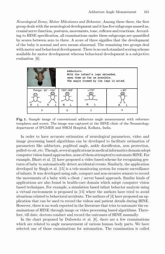
Adductors Angle Measurement 161
Neurological Items, Motor Milestones and Behavior. Among these three, the firstgroup deals with the neurological development and it has five subgroups named as,cranial nerve function, postures, movements, tone, reflexes and reactions. Accord-ing to HINE specification, all examinations under these subgroups are quantifiedby scores between zero to three. A score of three signifies that the developmentof the baby is normal and zero means abnormal. The remaining two groups dealwith motor and behavioral development. There is no such standard scoring schemeavailable for motor development whereas behavioral development is a subjectiveevaluation [6].
Fig. 1. Sample image of conventional adductors angle measurement with referencetemplates and scores. The image was captured at the HINE clinic of the Neonatologydepartment of IPGMER and SSKM Hospital, Kolkata, India.
In order to have accurate estimation of neurological parameters, video andimage processing based algorithms can be developed to facilitate estimation ofparameters like adductors, popliteal angle, ankle dorsiflexion, arm protection,pulled-to-sit, etc.Though, several applications inmedical informatics domainadoptcomputer visionbased approaches, noneof themattempted to automateHINE.Forexample, Bhatt et al. [2] have proposed a video based scheme for recognizing ges-tures of baby to automatically detect accidental events. Similarly, the applicationdeveloped by Singh et al. [15] is a tele-monitoring system for remote surveillanceof infants. It was developed using safe, compact and non-invasive sensors to recordthe movements of a baby with a client / server based approach. Similar kinds ofapplications are also found in health-care domain which adopt computer visionbased techniques. For example, a simulation based infant behavior analysis usinga virtual environment is proposed in [14] where the authors have tried to avoidsituations related to behavioral accidents. The authors of [4] have proposed an ap-plication that can be used to record the videos and patient details during HINE.However, there is no work reported in the literature that tries to automate the ex-aminations of HINE through image or video processing based algorithms. There-fore, till date, doctors conduct and record the outcomes of HINE manually.
In the chart proposed by Dubowitz et al. [6], there are a few examinationswhich are related to angle measurement of various human body parts. We haveselected one of those examinations for automation. The examination is called

162 D.P. Dogra et al.
as adductors angle measurement. In Fig. 1, a sample image of the scene duringadductors angle measurement is shown with reference templates and scores. Ithas been observed that during examinations involving measurement of variousangles, especially adductors angle and popliteal angle, the examiner often findsit difficult to keep the baby in a stable state. Since the baby moves frequently,placing a ruler across body parts for angle measurements become difficult. Inaddition to that, often the baby starts showing sign of uneasiness during theseexaminations. This has motivated us to design image processing based algorithmsto help the doctors during angle measurement examinations.
2 Proposed Angle Measurement Scheme
During adductors examination, the angle between the thighs of the infant at supineposture is measured and a score is assigned according to the reference templates(refer to Fig. 1). In the conventional approach, the examiner stretches the legs ofthe infant and rulers are used to measure the angle between the thighs as shownin the figure. An image based automatic scheme is proposed in this work. Aftersurveying the HINE clinic of the Neonatology department of Institute of The Post-Graduate Medical Education & Research (IPGMER) and Seth Sukhlal KarnaniMemorial (SSKM) Hospital, Kolkata, India, it was observed that a single camerais sufficient to capture the scene of the examination.The examinationdesk has beencovered with soft mattress. This was done in accordance with the well establishedsetup of the HINE clinic of the hospital. Normally, all clothings are removed fromthe baby before examination commences. Since the measurement of the adductorsangle is recorded only when the expert feels first resistance from the infant whilestretching the legs, we have captured one image per baby.
2.1 Segmentation and Binarization of Image
Estimation of adductors angle can be automated using the following image pro-cessing steps. First, a color based segmentation algorithm is used to distinguishbetween the background and foreground parts. Since the background is controlled,a color based separation is possible. We have tested with various popular imagesegmentation schemes that are commonly used for natural image segmentation [3],[8]–[11]. Performance of mean-shift based segmentation scheme proposed by Co-maniciu et al. [3] for the images of the domain under consideration has been foundto be satisfactory. Also, the authors of [5] and [12] have shown in their work thatmean-shift outperforms other algorithms in terms of quality. After segmentation,small and insignificant regions are merged with surrounding regions of larger sizeand importance (see Fig. 2b). To separate the foreground object (infant at supineand hands of the examiner) from the background, region that is dominated byhuman skin color is selected. A binary image is produced where the black pixelsrepresent foreground and white pixels represent background (see Fig. 2c).
2.2 Skeletonization of Binary ObjectNext, a widely used thinning scheme based on safe point thinning algorithm(SPTA) [13] is applied on the foreground objects. SPTA iteratively removes the
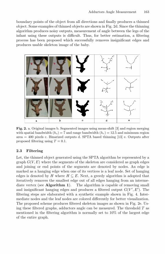
Adductors Angle Measurement 163
boundary points of the object from all directions and finally produces a thinnedobject. Some examples of thinned objects are shown in Fig. 2d. Since the thinningalgorithm produces noisy outputs, measurement of angle between the legs of theinfant using these outputs is difficult. Thus, for better estimation, a filteringprocess has been proposed which successfully removes insignificant edges andproduces usable skeleton image of the baby.
Fig. 2. a. Original images b. Segmented images using mean-shift [3] and region mergingwith spatial bandwidth (hs) = 7 and range bandwidth (hr) = 12.5 and minimum regionarea = 400 pixels c. Binarized outputs d. SPTA based thinning [13] e. Outputs afterproposed filtering using T = 0.1.
2.3 Filtering
Let, the thinned object generated using the SPTA algorithm be represented by agraph G(V, E) where the segments of the skeleton are considered as graph edgesand joining or end points of the segments are denoted by nodes. An edge ismarked as a hanging edge when one of its vertices is a leaf node. Set of hangingedges is denoted by H where H ⊆ E. Next, a greedy algorithm is adopted thatiteratively removes the smallest edge out of all edges hanging from an interme-diate vertex (see Algorithm 1). The algorithm is capable of removing smalland insignificant hanging edges and produces a filtered output G(V ′, E′). Thefiltering steps are elaborated with a synthetic example shown in Fig. 4. Inter-mediate nodes and the leaf nodes are colored differently for better visualization.The proposed scheme produces filtered skeleton images as shown in Fig. 2e. Us-ing these filtered graphs, adductors angle can be measured. The threshold T asmentioned in the filtering algorithm is normally set to 10% of the largest edgeof the entire graph.

164 D.P. Dogra et al.
Input: Skeleton produced by SPTA G(V, E)Output: Filtered output G(V, E)forall h ∈ H do1
if length(h) < T then2
H = H − h;3
E = E − h;4
forall h1 ∈ H AND h2 ∈ H do5
if h1 AND h2 are connected to same intermediate vertex then6
if length(h1) > length(h2) then7
E = E − h1;8
else9
E = E − h2;10
if No change in the graph in successive iterations then11
Stop the algorithm and return G(V, E);12
Algorithm 1. Filtering after SPTA based skeletonization
Fig. 3. Outputs at various intermediate steps of the filtering process a. Initial skeletonb. Intermediate skeleton c. Final skeleton.
2.4 Adductors Angle Measurement
The reduced graph generated by Algorithm 1 is used for estimating adductorsangle. In the graph, we search for the intermediate node A of G(V ′, E′) as shownin Fig. 3c. It is expected to be the joining point between two thighs since thebaby is placed supine with an upside down view with respect to camera. Next,two straight lines are fitted along the edges representing the thighs of the babyusing least square approximation method. Finally, the angle between the straightline segments denoted by AB and AC is estimated (refer to Fig. 3c).
3 Results and Discussions
We have recorded visuals of adductors angle measurement for 50 babies at theHINE clinic of SSKM hospital. Out of these 50 cases, the proposed filteringalgorithm was capable of generating usable skeletons for 46 images. Comparativeresults using the proposed scheme with respect to ground truths are shown inFig. 4. We have plotted the ground truths recorded by the experts and anglemeasured by the proposed scheme in the graph. In the graph, x-axis and y-axisdenote sample number and angle in degree. It is evident from the graph thatthe results agree with ground truth measurements (angle measured by doctors)

Adductors Angle Measurement 165
for majority of the samples. In the next part of the analysis, classification withrespect to ground truth scores is presented (see Table 1).
20
40
60
80
100
120
140
160
180
0 5 10 15 20 25 30 35 40 45 50
Addu
ctors
Angle
(in de
gree)
Sample Number
Doctor’s Measurement Automatic Measurement
Fig. 4. Comparison of automatic measurement with respect to ground truths recordedduring adductors angle measurement at SSKM hospital.
Since the scoring is done based on a range of angles, effect of errors in estimatingthe scores is less. Thus, high precision and recall is achieved. Fig. 5 shows someresults of abductors angle measurement. For better visualization, we have drawntwo thick straight lines (colored white) along the thighs of the baby and measuredthe angle between them.
Table 1. Classification of Results with respect to Recommended Scores of the HINEChart
80o < θ < 150o 150o < θ < 170o θ < 80o
Score: 3 Score: 2 Score: 0
GT(46) 33 6 7Outcomes TP FP FN TP FP FN TP FP FN
32 1 1 6 1 0 7 1 0Precision 96.96% 85.71% 87.5%Recall 96.96% 100% 100%
GT: Ground Truth, TP: True Positive, FP: False Positive, FN: False Negative
Fig. 5. Results of abductors angle measurement on some of the sample images collectedfrom IPGMER and SSKM Hospital
4 Conclusion and Future Directions
In this work, an image processing based algorithm has been proposed that can beused to measure the adductors angle of infants during HINE. This can be used to

166 D.P. Dogra et al.
automate the neurological assessment process. Since rulers and other measuringinstruments have to be used in a conventional approach, an automated schemewill reduce the workload of the examiner to a considerable extent. Though, in afew cases, our algorithm fails to measure the angle precisely, identifying range ofangle instead of exact value is possible with high accuracy. Other examinationslike measuring the popliteal angle, curvature in ventral suspension and ankledorsiflexion can be automated using similar techniques.
Acknowledgement
The work has been funded by Ministry of Communication and Information Tech-nology, Department of Information Technology, Govt. of India, under ApprovalNo. 1(4)/2009-ME& TMD (28-08-2009).
References
1. Arbelaez, P., Maire, M., Fowlkes, C., Malik, J.: From Contours to Regions: AnEmpirical Evaluation. In: CVPR, pp. 2294–2301 (2009)
2. Bhatt, J., Bebis, G.: Automatic Recognition of a Baby Gesture. In: ICTAI, pp.610–615 (2003)
3. Comaniciu, D., Meer, P.: Mean Shift: A Robust Approach Toward Feature SpaceAnalysis. IEEE Transactions on Pattern Analysis and Machine Intelligence 24(5),603–619 (2002)
4. Dogra, D., Nandam, K., Majumdar, A., Sural, S., Mukherjee, J., Mukherjee, S.,Singh, A.: A User Friendly Implementation for Efficiently Conducting Hammer-smith Infant Neurological Examination. In: Healthcom, pp. 374–378 (2010)
5. Dogra, D.P., Majumdar, A.K., Sural, S.: Evaluation of Segmentation TechniquesUsing Region Size and Boundary Information. In: Chaudhury, S., Mitra, S.,Murthy, C.A., Sastry, P.S., Pal, S.K. (eds.) PReMI 2009. LNCS, vol. 5909, pp.285–290. Springer, Heidelberg (2009)
6. Dubowitz, L., Dubowitz, V.: The Neurological Assessment of the Preterm and FullTerm Infant. Clinics in Developmental Medicine 9 (1981)
7. Felzenszwalb, D.: Efficient Graph-based Image Segmentation. International Journalof Computer Vision 59(2), 167–181 (2004)
8. Kuan, Y., Kuo, C., Yang, N.: Color-Based Image Salient Region SegmentationUsing Novel Region Merging Strategy. IEEE Transactions on Multimedia 10(5),832–845 (2008)
9. Martin, D.: An Empirical Approach to Grouping and Segmentation. Ph.D. Disser-tation, Univ. of California, Berkeley (2002)
10. Pal, N.R., Pal, S.K.: A Review on Image Segmentation Techniques. Journal ofPattern Recognition 26(9), 1277–1294 (1993)
11. Shi, J., Malik, J.: Normalized Cuts and Image Segmentation. IEEE Transactionson Pattern Analysis and Machine Intelligence 22(8), 888–905 (2000)
12. Unnikrishnan, R., Pantofaru, C., Hebert, M.: Toward Objective Evaluation of Im-age Segmentation Algorithms. IEEE Transactions on Pattern Analysis and Ma-chine Intelligence 29(6), 929–944 (2007)
13. Naccache, N., Shinghal, R.: SPTA: A Proposed Algorithm for Thinning Binary Pat-terns. IEEE Transactions on Systems Man and Cybernatics 14(3), 409–418 (1984)
14. Nishida, Y., Motomura, Y.: Infant Behavior Simulation Based on an EnvironmentalModel and a Developmental Behavior Model. ICSMC 2, 1555–1560 (2004)
15. Singh, S., Hsiao, H.: Infant Telemonitoring System. In: ICEMBS, pp. 1354–1357(2003)
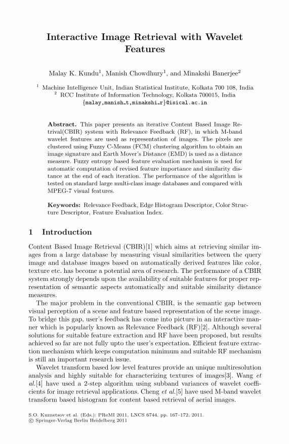
Interactive Image Retrieval with Wavelet
Features
Malay K. Kundu1, Manish Chowdhury1, and Minakshi Banerjee2
1 Machine Intelligence Unit, Indian Statistical Institute, Kolkata 700 108, India2 RCC Institute of Information Technology, Kolkata 700015, India
malay,manish t,minakshi [email protected]
Abstract. This paper presents an iterative Content Based Image Re-trival(CBIR) system with Relevance Feedback (RF), in which M-bandwavelet features are used as representation of images. The pixels areclustered using Fuzzy C-Means (FCM) clustering algorithm to obtain animage signature and Earth Mover’s Distance (EMD) is used as a distancemeasure. Fuzzy entropy based feature evaluation mechanism is used forautomatic computation of revised feature importance and similarity dis-tance at the end of each iteration. The performance of the algorithm istested on standard large multi-class image databases and compared withMPEG-7 visual features.
Keywords: Relevance Feedback, Edge Histogram Descriptor, Color Struc-ture Descriptor, Feature Evaluation Index.
1 Introduction
Content Based Image Retrieval (CBIR)[1] which aims at retrieving similar im-ages from a large database by measuring visual similarities between the queryimage and database images based on automatically derived features like color,texture etc. has become a potential area of research. The performance of a CBIRsystem strongly depends upon the availability of suitable features for proper rep-resentation of semantic aspects automatically and suitable similarity distancemeasures.
The major problem in the conventional CBIR, is the semantic gap betweenvisual perception of a scene and feature based representation of the scene image.To bridge this gap, user’s feedback has come into picture in an interactive man-ner which is popularly known as Relevance Feedback (RF)[2]. Although severalsolutions for suitable feature extraction and RF have been proposed, but resultsachieved so far are not fully upto the user’s expectation. Efficient feature extrac-tion mechanism which keeps computation minimum and suitable RF mechanismis still an important research issue.
Wavelet transform based low level features provide an unique multiresolutionanalysis and highly suitable for characterizing textures of images[3]. Wang etal.[4] have used a 2-step algorithm using subband variances of wavelet coeffi-cients for image retrieval applications. Cheng et al.[5] have used M-band wavelettransform based histogram for content based retrieval of aerial images.
S.O. Kuznetsov et al. (Eds.): PReMI 2011, LNCS 6744, pp. 167–172, 2011.c© Springer-Verlag Berlin Heidelberg 2011
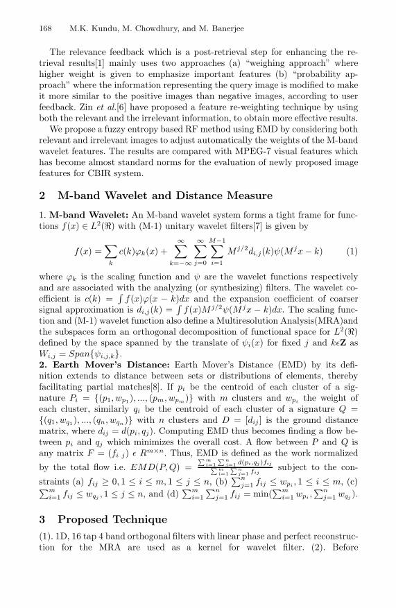
168 M.K. Kundu, M. Chowdhury, and M. Banerjee
The relevance feedback which is a post-retrieval step for enhancing the re-trieval results[1] mainly uses two approaches (a) “weighing approach” wherehigher weight is given to emphasize important features (b) “probability ap-proach” where the information representing the query image is modified to makeit more similar to the positive images than negative images, according to userfeedback. Zin et al.[6] have proposed a feature re-weighting technique by usingboth the relevant and the irrelevant information, to obtain more effective results.
We propose a fuzzy entropy based RF method using EMD by considering bothrelevant and irrelevant images to adjust automatically the weights of the M-bandwavelet features. The results are compared with MPEG-7 visual features whichhas become almost standard norms for the evaluation of newly proposed imagefeatures for CBIR system.
2 M-band Wavelet and Distance Measure
1. M-band Wavelet: An M-band wavelet system forms a tight frame for func-tions f(x) ∈ L2() with (M-1) unitary wavelet filters[7] is given by
f(x) =∑
k
c(k)ϕk(x) +∞∑
k=−∞
∞∑
j=0
M−1∑
i=1
M j/2di,j(k)ψ(M jx − k) (1)
where ϕk is the scaling function and ψ are the wavelet functions respectivelyand are associated with the analyzing (or synthesizing) filters. The wavelet co-efficient is c(k) =
∫f(x)ϕ(x − k)dx and the expansion coefficient of coarser
signal approximation is di,j(k) =∫
f(x)M j/2ψ(M jx − k)dx. The scaling func-tion and (M-1) wavelet function also define a Multiresolution Analysis(MRA)andthe subspaces form an orthogonal decomposition of functional space for L2()defined by the space spanned by the translate of ψi(x) for fixed j and kεZ asWi,j = Spanψi,j,k.2. Earth Mover’s Distance: Earth Mover’s Distance (EMD) by its defi-nition extends to distance between sets or distributions of elements, therebyfacilitating partial matches[8]. If pi be the centroid of each cluster of a sig-nature Pi = (p1, wp1), ..., (pm, wpm) with m clusters and wpi the weight ofeach cluster, similarly qi be the centroid of each cluster of a signature Q =(q1, wq1), ..., (qn, wqn) with n clusters and D = [dij ] is the ground distancematrix, where dij = d(pi, qj). Computing EMD thus becomes finding a flow be-tween pi and qj which minimizes the overall cost. A flow between P and Q isany matrix F = (fi j) ε Rm×n. Thus, EMD is defined as the work normalized
by the total flow i.e. EMD(P, Q) =∑ m
i=1∑ n
j=1 d(pi,qj)fij∑ mi=1
∑ nj=1 fij
subject to the con-
straints (a) fij ≥ 0, 1 ≤ i ≤ m, 1 ≤ j ≤ n, (b)∑n
j=1 fij ≤ wpi , 1 ≤ i ≤ m, (c)∑mi=1 fij ≤ wqj , 1 ≤ j ≤ n, and (d)
∑mi=1
∑nj=1 fij = min(
∑mi=1 wpi ,
∑nj=1 wqj ).
3 Proposed Technique
(1). 1D, 16 tap 4 band orthogonal filters with linear phase and perfect reconstruc-tion for the MRA are used as a kernel for wavelet filter. (2). Before

Interactive Image Retrieval with Wavelet Features 169
decomposing the image, RGB color plane of the image is converted into YCbCrcolor plane. (3). After color plane tranformation, each image plane is decomposedinto M×M channels without downsampling and then energy feature at each pixelis computed. (4). FCM clustering algorithm is used in each pixel to obtain the sig-nature. (5). EMD distance is computed between the query image and the storedimage signature in the database and the images are displayed in the first pass. (6).Feature Evaluation Index (FEI) are calculated from the marked relevant and ir-relevant set of images and recomputes the weighted EMD over each iteration.
3.1 Color-Texture Feature as Signature
Motivated from the idea that human visual system divides an image into severalbands, than actually visualizing the complete image as a whole. M-band waveletfilters are used which are essentially frequency and direction oriented band passfilters. Wavelet transform is applied to Y, Cb and Cr planes where decomposi-tion over the intensity plane characterizes texture and over chromaticity planescharacterizes color. For each of 16 subbands, absolute Gaussian energy for eachpixel is computed over a neighborhood and the size of which is determined usinga spectral flatness measure(SFM) given by the ratio of arithmetic mean and thegeometric mean of the Fourier coefficients of the image.
energym1,m2(i, j) =N∑
a=1
N∑
b=1
|Wfm1,m2(a, b)|G(i − a, j − b), (2)
Here, N is the neighborhood size and 1 ≤ m1 ≤ M, 1 ≤ m2 ≤ M whileWfm1,m2 is the wavelet transform coefficient obtained by row-wise convolutionusing the filter Hm1 and column-wise convolution with the filter Hm2 . The non-linear transform is succeeded by a Gaussian low-pass (smoothing) filter of the
form G(x, y) = 1√2πσ
e−(1/2σ2)(x2+y2), where σ defines the spatial extent of theaveraging filter. We use a neighborhood size of 11×11 for SFM between 1 and0.65, 21×21 for SFM between 0.65 and 0.35 while 31×31 for 0 to 0.35.
3.2 Iterative Computation of Weighted Based on Feature Relevance
Perceptual importance as used in the JPEG 2000 is Y : Cb : Cr = 4 : 2 : 1.Here, the weights are chosen heuristically. However, an automatic scheme whichchooses the weights depending on the color-texture complexity of the image willcertainly boost the performance of the CBIR system.
Combining information of relevant and irrelevant images marked by the users,the fuzzy features evaluation index (FEI) is computed considering a pattern clas-sification problem. If C1, C2, ..., Cm are m pattern classes in N dimensional fea-tures space where class Cj contains, nj number of samples. The features valuesalong the qth co-ordinate along classes Cj are assigned as standard S-type mem-bership function between 0 and 1[9]. Entropy(H) of Cj gives the measure of in-traset ambiguity is given as H(A) = ( 1
nj ln 2)∑
i Sn(μ(fiqj)); i = 1, 2...nj, whereSn(μ(fiqj))=-μ(fiqj)lnμ(fiqj)-1-μ(fiqj)ln1-μ(fiqj) is the Shannon’s function(μ). Hmin = 0 for μ=0 or 1, Hmax = 1 for μ=0.5.

170 M.K. Kundu, M. Chowdhury, and M. Banerjee
The FEIq for the qth component is defined as FEIq = Hqjk
Hqj+Hqk. Hqk is the en-
tropy of class Ck along qth dimension over nk number of samples. Hqjk(intersetambiguity) is entropy along qth dimension combining classes Cj and Ck with(nj + nk) number of samples. Lower value of FEIq, indicates better quality ofimportance of the qth feature because FEIq should be decreasing after com-bining Cj and Ck as the goodness of the qth features in descriminating patternclasses Cj and Ck increases[9]. The weight wq is a function of the evaluated(FEIq) is wq = Fq(FEIq).
Hqj is computed from the set of relevant images I(q)r = I(q)
r1 , I(q)r2 , I
(q)r3 ,...,I(q)
rk .Similarly, Hqk is computed from the set of irrelevant images where, I
(q)ir =I(q)
ir1,I(q)ir2, I
(q)ir3,...,I
(q)irk. Hqkj is computed combining both the sets. Images are ranked
according to EMD distance. The user marks the relevant and irrelevant set from20 returned images, for automatic evaluation of FEI.
Presently an image I is represented as a signature P = (p1, wp1 ), (p2, wp2), ..., (pm, wpm) = (pi, wpi)m
i=1with m clusters. The cluster centroid pi con-stitutes the wavelet features over 16 subbands of each Y, Cb and Cr planeand obtained with pi = [piY , piCb
, piCr ] which may be further represented as[f1Y , ..., fnY , f1Cb, ..., fnCb, f1Cr, ..., fnCb]. Here piY , piCb
and piCr are the localenergy values computed overall subbands of each Y, Cb and Cr planes respec-tively, for e.g piY = [f1Y , ..., fnY ] where piεR
N and N = 3n is the feature di-mension. Here n = 16 and wi ≥ 0.
The features considered to compute the feature evaluation index along eachcomponent plane for e.g plane Y are FY = fi1Y , ..., fiqY , where i = 1, 2, ..., m(m clusters) and q = 1, 2, ..., n (n subband features). Similarly features are con-sidered for Cb and Cr plane. The FEIqY for the component feature q of Y
plane are FEIqY = Hqtotal
HqRel+HqIrrel. Here, HqRel, HqIrrel and Hqtotal are the en-
tropies along the qth dimension of relevant, irrelevant and total returned imagesrespectively. And the (FEI)qCb and (FEI)qCr of other two planes are com-puted similarly. The overall weight factor for the Y plane is given by W ′
Y =∑mi=1
∑nq=1(FEI)qY , similarly W ′
Cb and W ′Cr are computed and the weight for
the Y plane is WY = W ′Y
W ′Y +W ′
Cb+W ′Cr
.Similarly WCb and WCr are computed. Multiplying with the weight actually
transforms the representative points pi but leave its distribution fixed. The EMDis now computed between the transformed signature maps. P ′ = g(pi), wpim
i=1
and Q′ = g(qj), wqjni=1, where pi and qi are the centroids of the query and
database images and g is the weight updating factor computed after each iter-ation. The EMDg(P, Q), where gε(WY , WCb, WCr) is computed from the workflow i.e. WORK(F, P
′, Q
′) =
∑mi=1
∑fi,jd(g(pi), g(qj)).
The transformed pi and qj is represented as p′i = [WY piY , WCbpiCb, WCrpiCr ]
and q′j = [WY qjY , WCbqjCb, WCrqjCr ] respectively. The EMD is computed upto
kth iteration till it converges i.e W (F (K+1), P′(K+1)K , Q
′(K+1)K ) ≤ W (F (K), P
′(K)K ,
Q′(K)K ). The signature maps for similar images are expected to be similar. After
multiplying with weights, the ranks of the relevant images are not affected much.
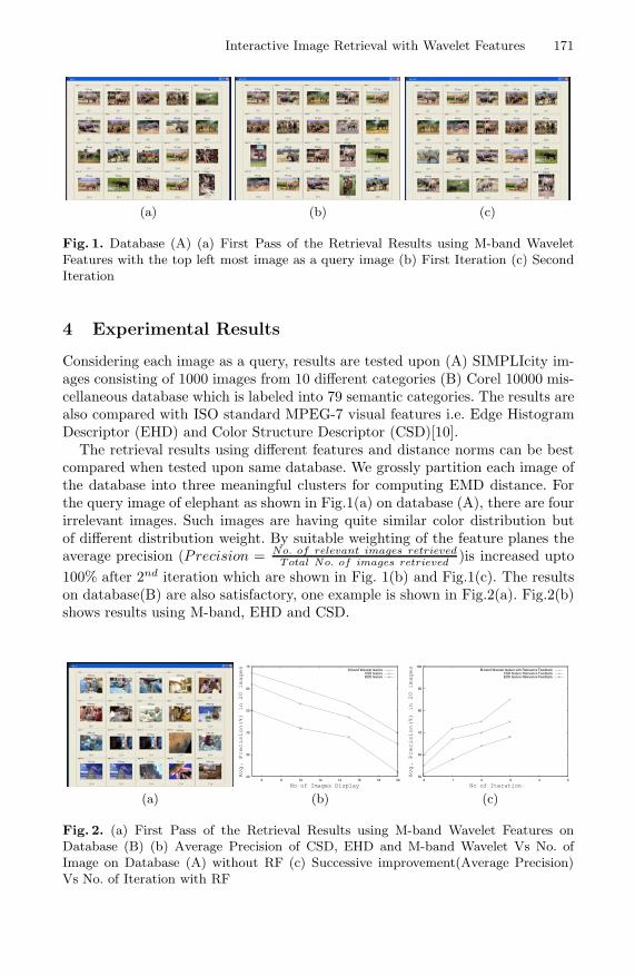
Interactive Image Retrieval with Wavelet Features 171
(a) (b) (c)
Fig. 1. Database (A) (a) First Pass of the Retrieval Results using M-band WaveletFeatures with the top left most image as a query image (b) First Iteration (c) SecondIteration
4 Experimental Results
Considering each image as a query, results are tested upon (A) SIMPLIcity im-ages consisting of 1000 images from 10 different categories (B) Corel 10000 mis-cellaneous database which is labeled into 79 semantic categories. The results arealso compared with ISO standard MPEG-7 visual features i.e. Edge HistogramDescriptor (EHD) and Color Structure Descriptor (CSD)[10].
The retrieval results using different features and distance norms can be bestcompared when tested upon same database. We grossly partition each image ofthe database into three meaningful clusters for computing EMD distance. Forthe query image of elephant as shown in Fig.1(a) on database (A), there are fourirrelevant images. Such images are having quite similar color distribution butof different distribution weight. By suitable weighting of the feature planes theaverage precision (Precision = No. of relevant images retrieved
Total No. of images retrieved )is increased upto100% after 2nd iteration which are shown in Fig. 1(b) and Fig.1(c). The resultson database(B) are also satisfactory, one example is shown in Fig.2(a). Fig.2(b)shows results using M-band, EHD and CSD.
20
30
40
50
60
70
6 8 10 12 14 16 18 20
Avg. Precision(%) in 20 images
No of Images Display
M-band Wavelet featureCSD featureEHD feature
50
60
70
80
90
100
0 1 2 3 4 5
Avg. Precision(%) in 20 images
No of Iteration
M-band Wavelet feature with Relevance FeedbackCSD feature Relevance FeedbackEHD feature Relevance Feedback
(a) (b) (c)
Fig. 2. (a) First Pass of the Retrieval Results using M-band Wavelet Features onDatabase (B) (b) Average Precision of CSD, EHD and M-band Wavelet Vs No. ofImage on Database (A) without RF (c) Successive improvement(Average Precision)Vs No. of Iteration with RF

172 M.K. Kundu, M. Chowdhury, and M. Banerjee
Fig. 2(c) shows an improvement in average precision (considering all databaseimages) upto 30% (maximum) at 3rd iteration using our RF with EMD on M-band wavelet features. Our results are found better than CSD and EHD whichshow an improvement of about 10% to 15% after 3rd iteration, where FEI isused with Euclidean distance.
MPEG-7 CSD visual features and M-band wavelet features approximatelytake 1-2 secs whereas EHD takes 500 ms. The CPU-time taken for each itera-tion is approximately 50 ms for database (A) and 3 sec for database (B) usingMATLAB R2008a on a Dell(T7400, 4GB, RAM) machine.
5 Conclusions
The proposed image retrieval system based on M-band wavelet features is able toimprove the retrieval performance satisfactorily within 2 to 3 iterations of rele-vance feedback. We intend to incorporate partial query using EMD and relevancefeedback in partial matching for videos in conjunction with motion informationas future scope of research.
References
1. Heesch, D.: A survey of browsing models for content based image retrieval. Multi-media Tools Application 40, 1380–7501 (2008)
2. Chang, F.C., Hang, H.M.: A relevance feedback image retrieval scheme using multi-instance and pseudo image concepts. IEICE Transaction Information System E89-D, 1720–1731 (2006)
3. Acharyya, M., Kundu, M.K.: An adaptive approach to unsupervised texture seg-mentation using M-band wavelet tranform. Signal Processing 81, 1337–1356 (2001)
4. Wang, J.Z., Li, J., Wiederhold, G.: Simplicity: Semantics-sensitive integratedmatching for picture libraries. IEEE Transactions on Pattern Analysis and Ma-chine Intelligence 23, 947–963 (2001)
5. Cheng, Q., Yang, C., Chen, F., Shao, Z.: Application of M-band wavelet theory totexture analysis in content-based aerial image retrieval. International Geoscienceand Remote Sensing Symposium 3, 2163–2165 (2004)
6. Jin, Z., King, I., Li, X.: Content-based image retrieval by relevance feedback. In:Laurini, R. (ed.) VISUAL 2000. LNCS, vol. 1929, pp. 521–529. Springer, Heidelberg(2000)
7. Burrus, C.S., Gopinath, A., Guo, H.: Introduction to Wavelets and Wavelet Trans-form: A Primer. Prentice Hall International Editions, Englewood Cliffs (1998)
8. Rubner, Y., Tomasi, C.: Perceptual Metrices for Image Database Navigation.Kluwer Academic Publishers, Boston (2001)
9. Pal, S.K., Majumder, D.D.: Fuzzy Mathematical Approach To Pattern Recogni-tion. Willey Eastern Limited, New York (1985)
10. Manjunath, B.S., Salembier, P., Sikora, T.: Introduction to MPEG-7: MultimediaContent Description Interface. John Wiley and Sons Inc., USA (2002)
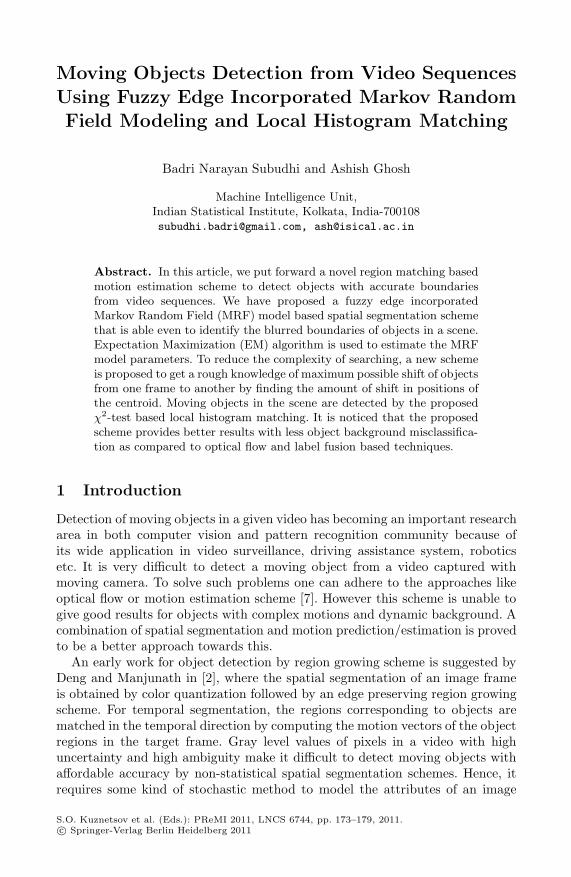
Moving Objects Detection from Video Sequences
Using Fuzzy Edge Incorporated Markov RandomField Modeling and Local Histogram Matching
Badri Narayan Subudhi and Ashish Ghosh
Machine Intelligence Unit,Indian Statistical Institute, Kolkata, [email protected], [email protected]
Abstract. In this article, we put forward a novel region matching basedmotion estimation scheme to detect objects with accurate boundariesfrom video sequences. We have proposed a fuzzy edge incorporatedMarkov Random Field (MRF) model based spatial segmentation schemethat is able even to identify the blurred boundaries of objects in a scene.Expectation Maximization (EM) algorithm is used to estimate the MRFmodel parameters. To reduce the complexity of searching, a new schemeis proposed to get a rough knowledge of maximum possible shift of objectsfrom one frame to another by finding the amount of shift in positions ofthe centroid. Moving objects in the scene are detected by the proposedχ2-test based local histogram matching. It is noticed that the proposedscheme provides better results with less object background misclassifica-tion as compared to optical flow and label fusion based techniques.
1 Introduction
Detection of moving objects in a given video has becoming an important researcharea in both computer vision and pattern recognition community because ofits wide application in video surveillance, driving assistance system, roboticsetc. It is very difficult to detect a moving object from a video captured withmoving camera. To solve such problems one can adhere to the approaches likeoptical flow or motion estimation scheme [7]. However this scheme is unable togive good results for objects with complex motions and dynamic background. Acombination of spatial segmentation and motion prediction/estimation is provedto be a better approach towards this.
An early work for object detection by region growing scheme is suggested byDeng and Manjunath in [2], where the spatial segmentation of an image frameis obtained by color quantization followed by an edge preserving region growingscheme. For temporal segmentation, the regions corresponding to objects arematched in the temporal direction by computing the motion vectors of the objectregions in the target frame. Gray level values of pixels in a video with highuncertainty and high ambiguity make it difficult to detect moving objects withaffordable accuracy by non-statistical spatial segmentation schemes. Hence, itrequires some kind of stochastic method to model the attributes of an image
S.O. Kuznetsov et al. (Eds.): PReMI 2011, LNCS 6744, pp. 173–179, 2011.c© Springer-Verlag Berlin Heidelberg 2011

174 B.N. Subudhi and A. Ghosh
frame so that a better segmentation result can be obtained. Markov RandomField (MRF) model, in this context, proved to be a better framework. A robustwork on MRF based object detection is demonstrated by Kuo et al. in [5], wherea combination of temporal and spatial constraints of the image frames are usedto obtain the moving object location from one frame to another of a video.Recently, Jodoin et al. [4] have proposed a robust moving object detection andtracking scheme for both fixed and moving camera captured video sequences,where MRF is used for label fields fusion. The label fields include two data:quickly estimated labels (i.e., a rough estimate of the location of object) and thespatial region map obtained by spatial segmentation with MRF model.
In this article, we propose a moving object detection scheme, that is able to de-tect moving objects with accurate object boundary from videos captured by mov-ing camera. The technique uses a region based motion estimation scheme. Here wehave proposed a new kind of MRF-MAP framework, where fuzzy edge strength ateach pixel is incorporated in the MRF modeling. The scheme is able to preservethe object boundary. The spatial segmentation problem is solved using the Maxi-mum a’posteriori probability (MAP) estimation principle. In region based motionestimation scheme, to reduce the complexity of searching, a rough knowledge ofmaximum possible shift in object from one frame to another is obtained by calcu-lating the amount of shift in the centroid of the object from one frame to another.Moving objects in the target frame is detected by χ2-test based local histogrammatching. It is observed that the proposed scheme provide better results with lessobject background misclassification as compared to existing techniques.
2 Spatial Segmentation Using Proposed Fuzzy EdgeIncorporated MRF Model
In this work it is assumed that the observed video sequence y is a 3-D volumeconsisting of spatio-temporal image frames. yt represents a video image frame attime t and hence is a spatial entity of size M ×N . Each pixel in yt is assumed asa site s denoted by yst. Let us assume that Xt represents the MRF from whichxt is a realization. Here Xt = Xt(i, j) is discrete valued and can take values fromQ = q1, q2, ..., qm. It is assumed here that due to the presence of noise (i.i.d)we are not able to observe Xt, and we observe a noisy version of Xt as Yt.
In spatial domain, Xt represents the MRF model of xt and using HamerselyClifford’s theorem the prior probability can be expressed as Gibb’s distribu-tion with P (Xt) = 1
ze
−U(xt)T , where z is the partition function expressed as
z =∑
xte
−U(xt)T , U(xt) is the energy function, a function of clique potentials
Vc(xt). According to Pott’s model the clique potential function Vc(xt) = −α ifall labels in possible set of cliques (C) are equal, otherwise Vc(xt) = +α. Equalpenalization of all the boundary pixels results in a greater penalty to weak edgepixels and a lesser penalty to the strong edge pixels. This results in improperidentification of boundary pixels in low resolution or blurred images. To reducethis effects one can adhere to the concept of incorporating local statistics basedkernel function in MRF model as U (xt) =
∑ηs
e−(xt⊗h). This defines the energy
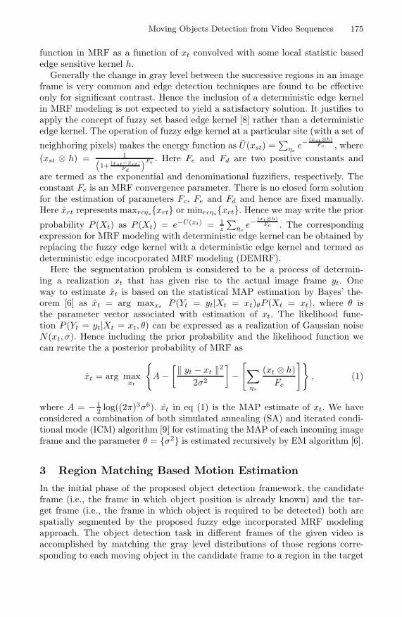
Moving Objects Detection from Video Sequences 175
function in MRF as a function of xt convolved with some local statistic basededge sensitive kernel h.
Generally the change in gray level between the successive regions in an imageframe is very common and edge detection techniques are found to be effectiveonly for significant contrast. Hence the inclusion of a deterministic edge kernelin MRF modeling is not expected to yield a satisfactory solution. It justifies toapply the concept of fuzzy set based edge kernel [8] rather than a deterministicedge kernel. The operation of fuzzy edge kernel at a particular site (with a set of
neighboring pixels) makes the energy function as U(xst) =∑
ηse−
(xst⊗h)Fc , where
(xst ⊗ h) = 1(1+
|xst−xrt|Fd
)Fe. Here Fe and Fd are two positive constants and
are termed as the exponential and denominational fuzzifiers, respectively. Theconstant Fc is an MRF convergence parameter. There is no closed form solutionfor the estimation of parameters Fc, Fe and Fd and hence are fixed manually.Here xrt represents maxrεηsxrt or minrεηsxrt. Hence we may write the prior
probability P (Xt) as P (Xt) = e−U(xt) = 1z
∑ηs
e−(xt⊗h)
Fc . The correspondingexpression for MRF modeling with deterministic edge kernel can be obtained byreplacing the fuzzy edge kernel with a deterministic edge kernel and termed asdeterministic edge incorporated MRF modeling (DEMRF).
Here the segmentation problem is considered to be a process of determin-ing a realization xt that has given rise to the actual image frame yt. Oneway to estimate xt is based on the statistical MAP estimation by Bayes’ the-orem [6] as xt = arg maxxt P (Yt = yt|Xt = xt)θP (Xt = xt), where θ isthe parameter vector associated with estimation of xt. The likelihood func-tion P (Yt = yt|Xt = xt, θ) can be expressed as a realization of Gaussian noiseN(xt, σ). Hence including the prior probability and the likelihood function wecan rewrite the a posterior probability of MRF as
xt = arg maxxt
A −
[‖ yt − xt ‖2
2σ2
]−
[∑
ηs
(xt ⊗ h)Fc
], (1)
where A = − 12
log((2π)3σ6). xt in eq (1) is the MAP estimate of xt. We haveconsidered a combination of both simulated annealing (SA) and iterated condi-tional mode (ICM) algorithm [9] for estimating the MAP of each incoming imageframe and the parameter θ = σ2 is estimated recursively by EM algorithm [6].
3 Region Matching Based Motion Estimation
In the initial phase of the proposed object detection framework, the candidateframe (i.e., the frame in which object position is already known) and the tar-get frame (i.e., the frame in which object is required to be detected) both arespatially segmented by the proposed fuzzy edge incorporated MRF modelingapproach. The object detection task in different frames of the given video isaccomplished by matching the gray level distributions of those regions corre-sponding to each moving object in the candidate frame to a region in the target

176 B.N. Subudhi and A. Ghosh
frame by χ2-test based histogram matching. To get an effective object detection,we propose an algorithm to find the rough estimation of maximum possible shiftin object from one frame to another by calculating the amount of shift in thecentroid of the object from one frame to another.
Calculation of Shift in Centroid and Local Histogram Matching: Letus consider two image frames at tth and (t + d)th instant of times, where the tth
frame is the candidate frame and (t+d)th frame is the target frame. Let us assumethat there are d numbers of moving objects in the scene, and their positions in thecandidate frame are known. From one frame to another as the object in the scenemove, there will be a shift in the centroid of the object. Considering the relativecamera movements in the scene as a multiplicative factor we can calculate theamount of shift of object in the scene as a function of distance. In the (t +d)th frame, the maximum possible shift of object in x-direction can be givenas shift(x,(t+d)b) = const ∗ max|Dist(t+d),b(i) − Distt,b(i)|b=1,2...d. Similarly,in y-direction it can be given as shift(y,(t+d)b) = const ∗ max|Dist(t+d),b(j) −Distt,b(j)|b=1,2...d. The Dist function represents distance of bth object centroidin the candidate frame to the target frame image centroid. The const representsa +ve constant that resolves the camera movements and scaling of the object inthe scene.
For matching each region corresponding to a moving object in the candidateframe to a region within the search space in the target frame, a search is made upto shift(x,(t+d)b) in the +ve and −ve directions of the x-axis and shift(y,(t+d)b)
in the +ve and −ve directions of the y-axis. Each time, we search a new regionin the target frame, the histogram corresponding to the new region is matchedwith a region corresponding to the object in the candidate frame by χ2-test[1]. By χ2-test based measure, the distribution/histogram of two regions can becompared by the formula,
χ2((h(bg,yt)), (h(g,y(t+d)))) =l=M−1∑
l=0
|(h(bg,yt)) − (h(g,y(t+d)))|(h(bg,yt)) + (h(g,y(t+d)))
.
The term h(bg,yt) represents the histogram corresponding to a region in bth objectof the candidate frame. The term h(g,y(t+d)) represents the histogram correspond-ing to a region within the search space (as obtained by centroid shifting scheme)in the target frame. Here g represents any region in the target frame withinthe obtained search space. M is the number of possible gray level bins in thehistogram.
4 Results and Discussion
The proposed scheme is tested on several video sequences, however for pageconstraint we have provided the results on one test video sequence. The resultsobtained by the proposed fuzzy edge map incorporated MRF modeling for spatialsegmentation is compared with those of the spatial segmentation by conventionalMRF modeling [4] and MRF modeling with deterministic edge kernel (DEMRF).Similarly, the moving object detection results obtained by the proposed schemeare compared with those obtained by optical flow [7] and label fusion [4] schemes.
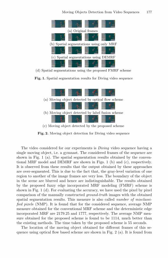
Moving Objects Detection from Video Sequences 177
(a) Original frames
(b) Spatial segmentations using only MRF
(c) Spatial segmentations using DEMRF
(d) Spatial segmentations using the proposed FMRF scheme
Fig. 1. Spatial segmentation results for Diving video sequence
(a) Moving object detected by optical flow scheme
(b) Moving object detected by label fusion scheme
(c) Moving object detected by the proposed scheme
Fig. 2. Moving object detection for Diving video sequence
The video considered for our experiments is Diving video sequence having asingle moving object, i.e. a gymnast. The considered frames of the sequence areshown in Fig. 1 (a). The spatial segmentation results obtained by the conven-tional MRF model and DEMRF are shown in Figs. 1 (b) and (c), respectively.It is observed from these results that the output obtained by these approachesare over-segmented. This is due to the fact that, the gray-level variation of oneregion to another of the image frames are very less. The boundary of the objectin the scene are blurred and hence are indistinguishable. The results obtainedby the proposed fuzzy edge incorporated MRF modeling (FMRF) scheme isshown in Fig. 1 (d). For evaluating the accuracy, we have used the pixel by pixelcomparison of the manually constructed ground-truth images with the obtainedspatial segmentation results. This measure is also called number of misclassi-fied pixels (NMP). It is found that for the considered sequence, average NMPmeasure obtained for the conventional MRF scheme and the deterministic edgeincorporated MRF are 2179.25 and 1777, respectively. The average NMP mea-sure obtained for the proposed scheme is found to be 1114, much better thanthe existing methods. The time taken by the proposed scheme is 55 seconds.
The location of the moving object obtained for different frames of this se-quence using optical flow based scheme are shown in Fig. 2 (a). It is found from

178 B.N. Subudhi and A. Ghosh
these results that the diving gymnast was not properly identified. Similarly,the moving object location obtained by the label fusion scheme are shown inFig. 2 (b). It is observed from these results that this technique is also not able toidentify the different parts of the gymnast correctly. However the results obtainedby the proposed scheme (as shown in Fig. 2 (c)) has correctly detected the gym-nast in different frames of the considered sequence. To evaluate the performanceof the detected moving object locations, we have considered the manually con-structed ground-truth based performance evaluation scheme of Erdem et al. [3].This scheme utilizes four different measures: misclassification penalty (Mi.P),motion penalty (M.P), shape penalty (S.P), and combined penalty (C.P) to eval-uate the performance of the moving objects locations. It may be noted that allthese measures should be low for better detection of moving objects. These mea-sures obtained for optical flow scheme are 0.5, 0.4, 0.4 and 0.45, respectively. Simi-larly these measure obtained for Label fusion scheme are 0.51, 0.38, 0.31 and 0.39,respectively. The results obtained for the proposed scheme are 0.42, 0.22, 0.22 and0.29, respectively. Thus the proposed scheme is seen to provide better results ascompared to the optical flow and label fusion schemes.
5 Conclusion
A new region based motion estimation scheme to detect moving objects fromgiven video sequences has been formulated. We have proposed a spatial seg-mentation technique by incorporating the fuzzy edge strength of pixels in MRFmodeling to preserve the object boundary. In this approach initially a roughestimate of object locations in the scene are obtained by finding the amountof shift in the centroid from one frame to another. The location of moving ob-jects in a scene is obtained by χ2-test based local histogram comparison. Theproposed scheme is found to be better as compared to the existing moving ob-ject detection schemes. The proposed scheme does not yield good results, withoclussion/dis-occlusion condition. In our future work we will try to solve theabove problem.
References
1. Ahonen, T., Hadid, A., Pietikainen, M.: Face recognition with local binary patterns.In: Pajdla, T., Matas, J(G.) (eds.) ECCV 2004. LNCS, vol. 3021, pp. 469–481.Springer, Heidelberg (2004)
2. Deng, Y., Manjunath, B.S.: Unsupervised segmentation of color-texture regions inimages and video. IEEE Transactions on Pattern Analysis And Machine Intelli-gence 23(8), 800–810 (2001)
3. Erdem, C.E., Sankur, B., Tekalp, A.M.: Performance measures for video objectsegmentation and tracking. IEEE Transactions on Image Processing 13(7), 937–951(2004)
4. Jodoin, P.M., Mignotte, M., Rosenberger, C.: Segmentation framework based onlabel field fusion. IEEE Transactions on Image Processing 16(10), 2535–2550 (2007)

Moving Objects Detection from Video Sequences 179
5. Kuo, C.M., Hsieh, C.H., Huang, Y.R.: Automatic extraction of moving objects forhead-shoulder video sequence. Journal of Visual Communication and Image Repre-sentation 16(1), 68–92 (2005)
6. Li, S.Z.: Markov Random Field Modeling in Image Analysis. Springer, Japan (2001)7. Lucas, B.D., Kanade, T.: An iterative image registration technique with an appli-
cation to stereo vision. In: Proceedings of Imaging understanding workshop, pp.121–130 (1981)
8. Pal, S.K., King, R.A.: On edge detection of x-ray images using fuzzy sets. IEEETransactions on Pattern Analysis Machine Intelligence 5(1), 69–77 (1983)
9. Subudhi, B.N., Nanda, P.K., Ghosh, A.: Moving object detection using MRF modeland entropy based adaptive thresholding. In: Proceedings of IEEE 2nd Interna-tional Conference on Human Computer Interaction, vol. 1, pp. 155–161. Springer,Heidelberg (2010)

Combined Topological and Directional RelationsBased Motion Event Predictions
Nadeem Salamat and El-hadi Zahzah
Université de La RochelleLaboratoire de Mathématiques, Images et Applications
Avenue M Crépeau La Rochelle 17042, Francensalam01,[email protected], [email protected]
Abstract. Spatial changes plays a fundamental role in modeling thespatio-temporal relations and spatio-temporal or motion event predic-tions. These predictions can be made through the conceptual neighbor-hood graph using the common sense continuity. This paper investigatesthat the extension in the temporal interval can effect the whole spatio-temporal relation and motion events. Spatio-temporal predicates form aunit of a motion event. We use the point temporal logic to extend thespatial predicates into the spatio-temporal or motion event predicates.
Keywords: Spatio-temporal relations, Spatial predicates, Spatio-temporal predictions, motion events.
1 Introduction
Spatio-temporal predictions are useful to initiate the new processus and to un-derstand a physical phenomenon, fundamentally the spatio-temporal predictionsare based on the predictions in the topological and directional relations [5,6,4].In these methods, topological relations are computed by 9-intersection model [7]or alternatively by Region Connected Calculus RCC8[3] and directional rela-tions are studied through method described in [10]. To fit the model in spatio-temporal context, an interval temporal logic[2] or point logic [9] are used. Anhybrid method for defining the spatio-temporal predicates is developed in [8],this method consider only topological changes and spatio-temporal predicatesare developed for moving objects.
Spatio-temporal motion event prediction is a process closely related to thespatio-temporal reasoning. The difference is, existing spatio-temporal reasoningprovide us information that a topological or directional relation exists at time t1,what is the possible topological or directional relation at time t2. In this paperwe define that if a spatio-temporal relation holds during an interval T , then howit will change spatio-temporal relation if an interval is extended and next timepoint is added to the interval.
The change in spatial scene is captured by the difference in topological, direc-tional and distance spatial relations between the snapshot taken at point t1 and
S.O. Kuznetsov et al. (Eds.): PReMI 2011, LNCS 6744, pp. 180–185, 2011.c© Springer-Verlag Berlin Heidelberg 2011

Combined Topological and Directional Relations 181
time point t2. This change in relative position may result change in topologi-cal, metric or orientation structure of an image. This requirement needs analysisin topological, metric and orientation viewpoint at each step and comparisonbetween two states, provided that both objects have a common lifetime.
Topological and directional relations are combined, method is argued in [13,14]and a complete Combined Topological and Directional relations (CTD) methodis developed in [11]. Graph of CTD method represents all binary topologicaldeformation in objects along with directional contents. In this graph, nodes rep-resent the topological and directional position of object pair and edge representsthe time. This neighborhood graph is used to predicate the spatio-temporal rela-tions. Next section explains the CTD method and section 3 describes the spatio-temporal prediction some examples are considered in section 4 and section 5concludes the paper.
2 CTD Method
1. Oriented lines, segments and longitudinal sections A and B be twospatial objects and (v, θ) ∈ R, Δθ(v) is an oriented line at θ. A∩Δθ(v) is theintersection of object A and Δθ(v), it is denoted by Aθ(v), called segment ofobject A and its length is x. Similarly length of Bθ(v) is z. y is the differencebetween minimum of A ∩ Δθ(v) and maximum of B ∩ Δθ(v). In case ofpolygonal object approximation (x, y, z) can be calculated from intersectingpoints of line and object’s boundary, oriented lines are considered which passthrough at least one vertex of two polygons. If there exist more than onesegment, it is called longitudinal section as in case of Aθ(v) in figure 1(a).
(a) Object pair and orientedline
(b) Neighborhood graph of Allen relations
Fig. 1. Black (dark grey) represents reference and light gray argument object
2. Allen temporal relations in spatial domain and fuzziness Allen[1]introduced 13 jointly exhaustive and pairwise disjoint (JEPD) interval rela-tions. These relations are arranged as A=<, m, o, s, f, d, eq, di, fi, si, oi, mi,> with meanings before, meet, overlap, start, finish, during, equal, during_by,finish_by, start_by, overlap_by, meet_by, and after. Allen relations in space
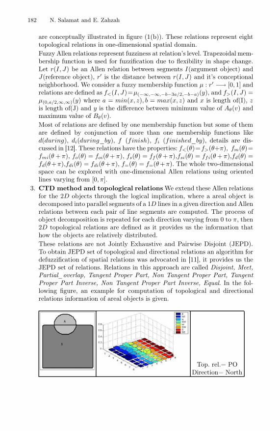
182 N. Salamat and E. Zahzah
are conceptually illustrated in figure (1(b)). These relations represent eighttopological relations in one-dimensional spatial domain.Fuzzy Allen relations represent fuzziness at relation’s level. Trapezoidal mem-bership function is used for fuzzification due to flexibility in shape change.Let r(I, J) be an Allen relation between segments I(argument object) andJ(reference object), r′ is the distance between r(I, J) and it’s conceptionalneighborhood. We consider a fuzzy membership function μ : r′ −→ [0, 1] andrelations are defined as f<(I, J)=μ(−∞,−∞,−b−3a/2,−b−a)(y), and f>(I, J) =μ(0,a/2,∞,∞)(y) where a = min(x, z), b = max(x, z) and x is length of(I), zis length of(J) and y is the difference between minimum value of Aθ(v) andmaximum value of Bθ(v).Most of relations are defined by one membership function but some of themare defined by conjunction of more than one membership functions liked(during), di(during_by), f (finish), fi (finished_by), details are dis-cussed in [12]. These relations have the properties: f<(θ)=f>(θ+π), fm(θ)=fmi(θ +π), fo(θ) = foi(θ + π), fs(θ) = ff (θ +π),fsi(θ) = ffi(θ + π),fd(θ) =fd(θ+π),fdi(θ) = fdi(θ+π), f=(θ) = f=(θ+π). The whole two-dimensionalspace can be explored with one-dimensional Allen relations using orientedlines varying from [0, π].
3. CTD method and topological relations We extend these Allen relationsfor the 2D objects through the logical implication, where a areal object isdecomposed into parallel segments of a 1D lines in a given direction and Allenrelations between each pair of line segments are computed. The process ofobject decomposition is repeated for each direction varying from 0 to π, then2D topological relations are defined as it provides us the information thathow the objects are relatively distributed.These relations are not Jointly Exhaustive and Pairwise Disjoint (JEPD).To obtain JEPD set of topological and directional relations an algorithm fordefuzzification of spatial relations was advocated in [11], it provides us theJEPD set of relations. Relations in this approach are called Disjoint, Meet,Partial_overlap, Tangent Proper Part, Non Tangent Proper Part, TangentProper Part Inverse, Non Tangent Proper Part Inverse, Equal. In the fol-lowing figure, an example for computation of topological and directionalrelations information of areal objects is given.
Top. rel.= PODirection= North
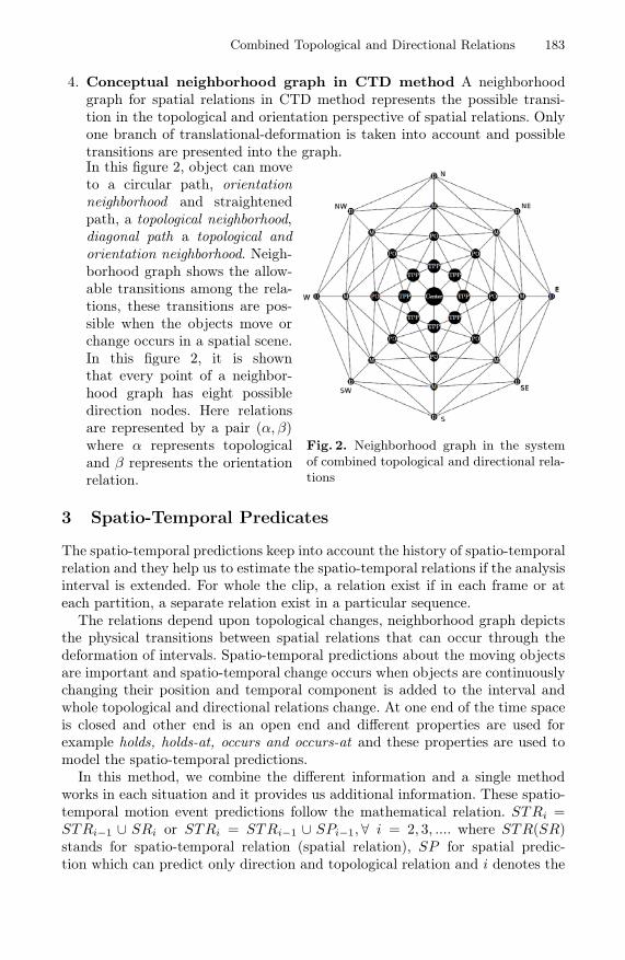
Combined Topological and Directional Relations 183
4. Conceptual neighborhood graph in CTD method A neighborhoodgraph for spatial relations in CTD method represents the possible transi-tion in the topological and orientation perspective of spatial relations. Onlyone branch of translational-deformation is taken into account and possibletransitions are presented into the graph.In this figure 2, object can moveto a circular path, orientationneighborhood and straightenedpath, a topological neighborhood,diagonal path a topological andorientation neighborhood. Neigh-borhood graph shows the allow-able transitions among the rela-tions, these transitions are pos-sible when the objects move orchange occurs in a spatial scene.In this figure 2, it is shownthat every point of a neighbor-hood graph has eight possibledirection nodes. Here relationsare represented by a pair (α, β)where α represents topologicaland β represents the orientationrelation.
Fig. 2. Neighborhood graph in the systemof combined topological and directional rela-tions
3 Spatio-Temporal Predicates
The spatio-temporal predictions keep into account the history of spatio-temporalrelation and they help us to estimate the spatio-temporal relations if the analysisinterval is extended. For whole the clip, a relation exist if in each frame or ateach partition, a separate relation exist in a particular sequence.
The relations depend upon topological changes, neighborhood graph depictsthe physical transitions between spatial relations that can occur through thedeformation of intervals. Spatio-temporal predictions about the moving objectsare important and spatio-temporal change occurs when objects are continuouslychanging their position and temporal component is added to the interval andwhole topological and directional relations change. At one end of the time spaceis closed and other end is an open end and different properties are used forexample holds, holds-at, occurs and occurs-at and these properties are used tomodel the spatio-temporal predictions.
In this method, we combine the different information and a single methodworks in each situation and it provides us additional information. These spatio-temporal motion event predictions follow the mathematical relation. STRi =STRi−1 ∪ SRi or STRi = STRi−1 ∪ SPi−1, ∀ i = 2, 3, .... where STR(SR)stands for spatio-temporal relation (spatial relation), SP for spatial predic-tion which can predict only direction and topological relation and i denotes the

184 N. Salamat and E. Zahzah
time at which the relations are evaluated. These relations can be reformulatedas STPi = STRi ∪ SPi,∀ i = 2, 3, .... here STP (SP ) represents the spatio-temporal (spatial) prediction and spatio-temporal relation at ith frame is thespatio-temporal prediction of (i − 1)th frame.
4 Examples
Motion is a continuous phenomenon, of course, it can be analyzed at a discon-tinuous time pints and between these two points it can be directly interpolated.These time points can be chosen at a predefined time intervals or a specificvideo frame called snapshot. In modeling the spatio-temporal relations and mo-tion events we need at least two snapshots, or two basic intervals where a stablespatial temporal relations hold. We start from two snapshots, at initial point,both spatio-temporal and spatial predictions represents the same semantics andpossible predicates are given in table 1.
Table 1. Spatio-temporal predictions for two frames
SR SP STR(D,N) (D,NE) Changing direction, getting closer or going away from N to NE(D,N) (D,N) getting closer or going away in N(D,N) (D,NW) getting closer or going away N to NW(D,N) (M,NE) Snap from NE(D,N) (M,N) Snap from N(D,N) (M,NW) Snap from NW
When the interval is extended, a new snapshot or a basic interval where thespatio-temporal relation is not changed is added to the interval.
Table 2. STR predictions for third frames
STRi−1 SPi−1 STRiorSTPi−1
Snap from NE D, E Touching form NESnap from NE M, E BypassSnap from NE PO, E Graze, Enter, Into from ESnap from NE D, NE Touch from NESnap from NE PO, NE Enter, Into from NESnap from NE D, N Touching from NESnap from NE M, N Bypass towards NSnap from NE PO, N Graze, Enter, Into from N
Spatial relations arerepresented in the neigh-borhood graph, every pointhas the eight possible spa-tial predictions. we dis-cuss here the possiblespatial predictions from(M,NE) and the exist-ing spatio-temporal rela-tion at this point is Snapfrom NE then the spatio-temporal predicates aredepicted in table 2. These spatio-temporal predicates depend upon the currentspatial predicates. Similarly, for other possibilities.
Combined Topological and Directional Relations 185
5 Conclusion
Spatio-temporal prediction is a closely related to the spatial reasoning methods.In this paper, it is discussed that if the interval for which a spatio-temporalrelation is analyzed is extended then it can effect the whole spatio-temporalrelation and motion events. In modeling the spatio-temporal predictions, spatialpredictions for topological and directional relations and neighborhood graphsare also important. Temporal domain is handled through the interval or pointtemporal logic. We used the topological and orientation information at the sametime and CTD method is used for binary topological and directional relationsbetween the object pair.
References
1. Allen, J.F.: Maintaining Knowledge about Temporal Intervals. Communications ofthe ACM 26(11), 832–843 (1983)
2. Allen, J.F., Ferguson, G.: Actions and Events in Interval Temporal Logic. Journalof Logic and Computation 4, 531–579 (1994)
3. Cohn, A.G., Bennett, B., Gooday, J., Gotts, N.: RCC: a Calculus for Region-BasedQualitative Spatial Reasoning. GeoInformatica 1, 275–316 (1997)
4. Cohn, A.G., Hazarika, S.M.: Qualitative Spatial Representation and Reasoning:An Overview. Fundamenta Informaticae 46(1-2), 1–29 (2001)
5. Egenhofer, M., Mark, D.: Modeling Conceptual Neighborhoods of Topological Line-Region Relations. International Journal of Geographical Information Systems 9,555–565 (1995)
6. Egenhofer, M.J., Al-Taha, K.K.: Reasoning about Gradual Changes of TopologicalRelationships. In: Proceedings of the International Conference On GIS - FromSpace to Territory, pp. 196–219. Springer, London (1992)
7. Egenhofer, M.J., Franzosa, R.D.: Point Set Topological Relations. InternationalJournal of Geographical Information Systems 5(2), 161–174 (1991)
8. Erwig, M., Schneider, M., Hagen, F., Praktische Informatik Iv.: Spatio-TemporalPredicates. IEEE Transactions on Knowledge and Data Engineering 14, 881–901(1999)
9. Galton, A.: A generalized topological view of motion in discrete space. Theor.Comput. Sci. 305(1-3), 111–134 (2003)
10. Goyal, R.K., Egenhofer, M.J.: Similarity of cardinal directions. In: Jensen, C.S.,Schneider, M., Seeger, B., Tsotras, V.J. (eds.) SSTD 2001. LNCS, vol. 2121, pp.36–58. Springer, Heidelberg (2001)
11. Salamat, N., Zahzah, E.h.: 2D Fuzzy Spatial Relations: New Way of Computingand Representation, http://hal.archives-ouvertes.fr/hal-00551281/en/
12. Salamat, N., Zahzah, E.h.: On the improvement of Combined topological and Di-rectional Relations Information,http://hal.archives-ouvertes.fr/hal-00551278/en/
13. Salamat, N., Zahzah, E.h.: Fusion of Fuzzy Spatial Relations. In: Proceedings ofThe 5th International Conference on Hybrid Artificial Intelligence Systems (HAIS(1)), pp. 294–301 (2010)
14. Salamat, N., Zahzah, E.h.: Fuzzy Spatial Relations For 2D Scene. In: Proceedingsof The 2010 International Conference on Image Processing, Computer Vision, andPattern Recognition (IPCV-2010), pp. 47–53 (2010)

Recognizing Hand Gestures of a Dancer
Divya Hariharan1, Tinku Acharya2, and Sushmita Mitra1
1 Machine Intelligence Unit, Indian Statistical Institute, Kolkata 700 108, [email protected]
2 Videonetics Technology Private Limited, Kolkata, [email protected]
Abstract. A new and simple two-level decision making system has beendesigned for performing scale-, translation- and rotation-invariant recog-nition of various single-hand gestures of a dancer. The orientation fil-ter is used at the first-level to generate a feature vector that is able todistinguish between several gestures. At the second-level the silhouetteof the different gestures is extracted, followed by the generation of thecorresponding skeleton and the evaluation of the gradients at its endpoints. These gradients constitute the second feature set, for recogniz-ing those gestures which remain to be identified at the first-level. Anapplication has been provided in the domain of single-hand gestures ofBharatanatyam, an Indian classical dance form.
Keywords: Gesture recognition, feature extraction, skeleton matching,orientation histogram.
1 Introduction
The term Indian Classical Dance comprises all the art forms of the Natyashastrawritten by the ancient musicologist Sage Bharata. The Natyashastra confersclassical status to eight Indian dances, of which Bharatanatyam is one of theoldest. A popular interpretation of the name isBHAva (expression) + RAga (musical mode) + TAla (rhythm) + NATYAM(dance) = BHARATANATYAM.
A distinctive feature of Bharatanatyam Dance is the use of expressive handgestures as a way of communication. Hastas [3] refers to a variety of hand symbolsthat a dancer can use. Hastas can be broadly classified into two categories, viz.,Asamyukta Hastas (Single hand gestures) and Samyukta Hastas (Double handgestures). There exist 28 Asamyukta Hastas and 24 Samyukta Hastas.
The objective of this research is to develop a suitable prototype for the recog-nition of the 28 Asamyukta Hastas of Bharatanatyam in a two dimensional space,using image processing techniques [1]. We aim to make the computer act as ateacher to correct the dance gestures, for the purpose of promoting e-learning ofthe nuances of Bharatanatyam across the world.
A major difficulty is associated with the rotation and scaling involved. Forexample, a gesture image rotated to any degree or scaled to any level should
S.O. Kuznetsov et al. (Eds.): PReMI 2011, LNCS 6744, pp. 186–192, 2011.c© Springer-Verlag Berlin Heidelberg 2011

Recognizing Hand Gestures of a Dancer 187
represent the same gesture. Orientation filters [2] have been used in various im-age processing and vision tasks, by applying filters of arbitrary orientation andphase. Typically a few filters, corresponding to a few angles, are employed andthe intermediate responses are interpolated. With a correct filter set and inter-polation rule, it becomes possible to evaluate a filter of any arbitrary orientation.
In this article we use the orientation filter at the first-level to generate afeature vector for distinguishing between different gestures. At the second-levelthe silhouette of the different gestures is extracted, followed by the generation ofthe corresponding skeleton and the evaluation of the gradients at its end points.This constitutes the second feature set, for recognizing those gestures whichremain to be identified at the first-level. The rest of the paper is organizedas follows. Section 2 describes the generation of the feature vector at the twolevels, comprising computation of the orientation histogram and the gradientsat the extremities of the hand. The experimental results are provided in detailin Section 3. Finally, Section 4 concludes the article.
2 Feature Extraction
The preprocessing of the hand gesture consists of detecting the skin color in theimage, and cropping the hand region in order to avoid unnecessary details inthe background. The images are then resized to 240 × 240 and converted togray scale. The next step is the feature extraction procedure. A suitable featurevector which is invariant to translation, rotation, scaling and reflection needs tobe chosen for the purpose of distinguishing between the different gestures.
2.1 Edge Orientation Histogram
Considering the aspects of translation and scaling invariance, the orientationhistogram [2] was found to be a useful feature component. Here these constitutehistograms of local orientation of the hand gesture. The orientation histogramsare robust to illumination changes, and are simple and fast to compute.
Local orientation is obtained by the use of steerable filters, in which a filterof arbitrary orientation is synthesized as a linear combination of a set of “basisfilters”. A set of 36 one-dimensional Gaussian steerable filters and their first orderderivatives have been used for extracting the local edge orientation propertiesof the hand gesture for every 10o, ranging from 0o to 350o. The gesture imageI, filtered at an arbitrary orientation and convolved with the filters, can besynthesized for the oriented filter response
Rθ1 = (G0o
1 ∗ I) cos θ + (G90o
1 ∗ I) sin θ, (1)
where ∗ represents the convolution operator, and Gθ1 is considered at an arbitrary
orientation θ.In order to enhance the ability of the edge orientation histogram in recognizing
the rotated gestures, the direction of maximum local orientation of every gestureis found. Accordingly the original gesture image is rotated in such a manner that
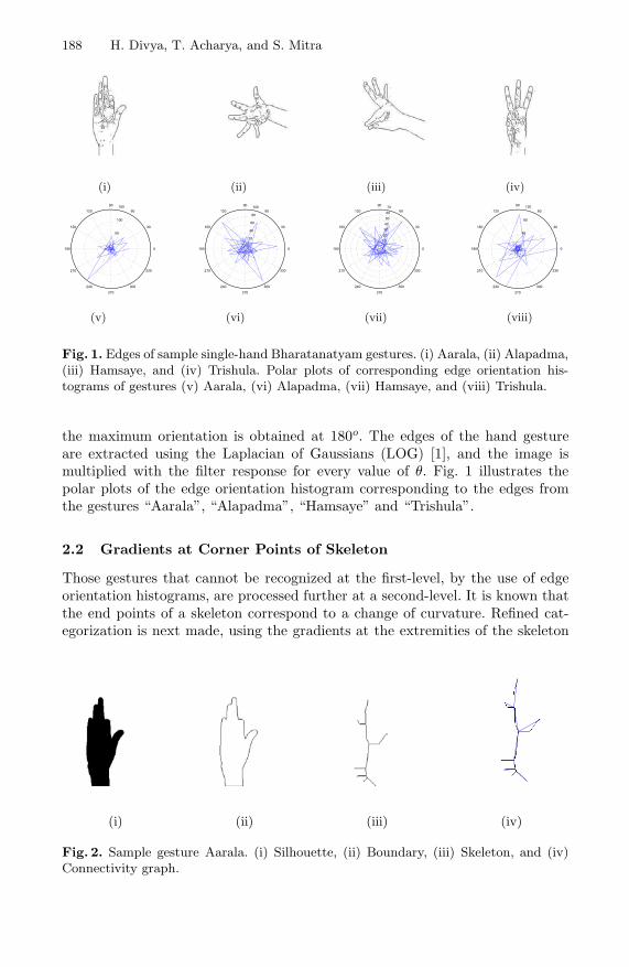
188 H. Divya, T. Acharya, and S. Mitra
(i) (ii) (iii) (iv)
50
100
150
30
210
60
240
90
270
120
300
150
330
180 0
20
40
60
80
100
30
210
60
240
90
270
120
300
150
330
180 0
10
20
30
40
50
60
70
30
210
60
240
90
270
120
300
150
330
180 0
40
80
120
30
210
60
240
90
270
120
300
150
330
180 0
(v) (vi) (vii) (viii)
Fig. 1. Edges of sample single-hand Bharatanatyam gestures. (i) Aarala, (ii) Alapadma,(iii) Hamsaye, and (iv) Trishula. Polar plots of corresponding edge orientation his-tograms of gestures (v) Aarala, (vi) Alapadma, (vii) Hamsaye, and (viii) Trishula.
the maximum orientation is obtained at 180o. The edges of the hand gestureare extracted using the Laplacian of Gaussians (LOG) [1], and the image ismultiplied with the filter response for every value of θ. Fig. 1 illustrates thepolar plots of the edge orientation histogram corresponding to the edges fromthe gestures “Aarala”, “Alapadma”, “Hamsaye” and “Trishula”.
2.2 Gradients at Corner Points of Skeleton
Those gestures that cannot be recognized at the first-level, by the use of edgeorientation histograms, are processed further at a second-level. It is known thatthe end points of a skeleton correspond to a change of curvature. Refined cat-egorization is next made, using the gradients at the extremities of the skeleton
(i) (ii) (iii) (iv)
Fig. 2. Sample gesture Aarala. (i) Silhouette, (ii) Boundary, (iii) Skeleton, and (iv)Connectivity graph.

Recognizing Hand Gestures of a Dancer 189
as a new set of features. A given gray scale image is initially binarized in a uni-form manner over hand gestures of different people. The boundary is extractedfrom the binary image, followed by the flood-fill operation to generate a uniformsilhouette. This is depicted in Fig. 2(i) for a sample dance gesture “Aarala”.
The skeleton [Fig. 2(iii)] is extracted by the morphological operation of thin-ning. Typically it consists of a number of branch points and end points, connectedby curve segments. These points are considered to be the nodes of a graph, suchthat the skeletal curve segments form the edges. This graph [Fig. 2(iv)] is calledthe connectivity graph of the skeleton. It provides topological information aboutthe hand gesture.
Matching of the connectivity graphs, based on their topologies and geometricfeatures, provides a distance measure for determining the similarity (or dissim-ilarity) between the different shapes. The adjacency matrix of the connectivitygraph is constructed. The degree of every node in the graph is computed and as-signed as its weight. Subsequently, a depth-first traversal sequence is constructedfor the connectivity graph starting from one end point (typically, the leftmostpoint). Preference is provided to a node with a lower weight during the traversal.Thereby, the number of backtracking sequences gets reduced.
Fig. 3. Depth-first traversal in edge connectivity graph of Aarala
The thick black lines in Fig. 3 indicate the depth-first traversal sequence ofthe connectivity graph of Fig. 2(iv). The sequence obtained is expressed as
G → F → I → H → I → K → J → K → L → K → I → F → D → E → D →C → B → C → A.
Repetitions of nodes correspond to the backtracking of edges during traversalof the graph.
For every end point in the skeleton, the nearest boundary point is obtained.Without loss of generality, it can be inferred that this nearest boundary pointwill be either a finger tip or a point in the hand gesture where the curvaturechange is large. Hence the gradient at these points will significantly vary overthe different gestures. For the branch points, this value is assigned to be zero in
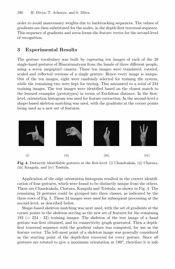
190 H. Divya, T. Acharya, and S. Mitra
order to avoid unnecessary weights due to backtracking sequences. The values ofgradients are then substituted for the nodes, in the depth-first traversal sequence.This sequence of gradients and zeros forms the feature vector for the second-levelof recognition.
3 Experimental Results
The gesture vocabulary was built by capturing ten images of each of the 28single-hand gestures of Bharatanatyam from the hands of three different people,using a seven megapixel camera. These ten images were translated, rotated,scaled and reflected versions of a single gesture. Hence every image is unique.Out of the ten images, eight were randomly selected for training the system,while the remaining two were kept for testing. This amounted to a total of 224training images. The test images were identified based on the closest match tothe learned examples (prototypes) in terms of Euclidean distance. In the first-level, orientation histogram was used for feature extraction. In the second-level ashape-based skeleton matching was used, with the gradients at the corner pointsbeing used as a new set of features.
(i) (ii) (iii) (iv)
Fig. 4. Distinctly identifiable gestures at the first-level. (i) Chandrakala, (ii) Chatura,(iii) Kangula, and (iv) Trishula.
Application of the edge orientation histogram resulted in the correct identifi-cation of four gestures, which were found to be distinctly unique from the others.These are Chandrakala, Chatura, Kangula and Trishula, as shown in Fig. 4. Theremaining 24 gestures could be grouped into three classes, as indicated by thethree rows of Fig. 5. These 24 images were used for subsequent processing at thesecond-level, as described below.
Shape-based skeleton matching was next used, with the set of gradients at thecorner points in the skeleton serving as the new set of features for the remaining192 (= 224 - 32) training images. The skeleton of the test image of a handgesture was first obtained, and its connectivity graph generated. Then a depth-first traversal sequence with the gradient values was computed, for use as thefeature vector. The left-most point of a skeleton image was generally consideredas the starting point of the depth-first traversal for every gesture. Since allgestures are rotated to give a maximum orientation at 180o, therefore it is safe

Recognizing Hand Gestures of a Dancer 191
(i) (ii) (iii) (iv) (v) (vi) (vii)
(viii) (ix) (x) (xi) (xii) (xiii) (xiv) (xv) (xvi)
(xvii) (xviii) (xix) (xx) (xxi) (xxii) (xxiii) (xxiv)
Fig. 5. Three groups of gestures at first-level. Class 1 with (i) Aarala, (ii) Ardhachan-dra, (iii) Ardhapataka, (iv) Mayura, (v) Pataka, (vi) Shukatunda, (vii) Tripataka. Class2 with (viii) Alapadma, (ix) Bhramara, (x) Kapitta, (xi) Katakamukha, (xii) Pad-makosha, (xiii) Sandamsha, (xiv) Shikara, (xv) Simhamukha, and (xvi) Suchi. Class3 with (xvii) Hamsaye, (xviii) Hansapakshika, (xix) Kartarimukha, (xx) Mrigashirsa,(xxi) Mukula, (xxii) Mushti, (xxiii) Sarpashirsa, and (xxiv) Tamrachuda.
to assume that for the same gesture the starting point will be the same. Thematching of two shapes now reduces to the problem of matching two featuresequences.
Let V and U be two such sequences of lengths n and m respectively. Usingconcepts from dynamic programming, a cost function Cost(i, j) is defined as thecost of matching the ith element Vi of the first sequence with the jth elementUj of the second sequence. It is defined as Cost(i, j) =
minCost(i, j−1), Cost(i−1, j), Cost(i−1, j−1)+Weight(Vi)×Vi−Weight(Uj)×Uj .( ) (2)
In order to match the sequences V and U , one needs to compute the cost overtheir entire length. It is evident that the value of the cost function determinesthe similarity (or dissimilarity) between the shapes of different hand gestures.There are, however, possibilities of error due to the irregularities in the skeletonstructure from the hands of different people with different textural properties.
After the second-level of processing only four of the gesture types remainedincorrectly recognized. These images are presented in Fig. 6, with the upper rowindicating the misclassified gesture and the lower depicting the correspondingcategory with which it has been mistaken. It can be easily observed that each ofthese image pairs, viz. those in lying in the same column of the figure, are highlysimilar to the human eye. Hence the performance of the designed system, on thewhole, can be claimed to be reasonably good.

192 H. Divya, T. Acharya, and S. Mitra
(i) (ii) (iii) (iv)
(v) (vi) (vii) (viii)
Fig. 6. Dance gestures still misclassified at the second-level. (i) Kartarimukha, (ii)Bhramara, (iii) Mrigashirsa, and (iv) Hansapakshika, were mistaken with (v) Pataka,(vi) Aarala, (vii) Sandamsha, and (viii) Padmakosha, respectively.
4 Conclusion
E-learning would be a very practical, simple and cost-effective mode of impart-ing training in the nuances of traditional dance across the globe, thereby assim-ilating the cultural divide between the Orient and the West. We aim to makethe computer act as a teacher to correct the dance gestures for the purposeof promoting classical Indian dance across the world. A simple and new two-level decision making system has been designed for recognizing the gestures ofBharatanatyam, a well-known Indian classical dance form. It has been shownto be scale-, translation- and rotation-invariant while recognizing various single-hand gestures of a dancer.
Acknowledgement. This research was carried out while Ms. D. Hariharan wasin ISI on an IASc-INSA-NASI summer fellowship.
References
1. Acharya, T., Ray, A.K.: Image Processing Principles and Applications. John Wiley,New Jersey (2005)
2. Freeman, W.T., Roth, M.: Orientation histograms for hand gesture recognition.In: Proceedings of IEEE International Workshop on Automatic Face and GestureRecognition, pp. 296–301. IEEE, Los Alamitos (1994)
3. Verma, M.: Bharatanatyam: Origin, Styles and Techniques, chap, pp. 295–315. Ab-hishek Publishers, Hastas (2009)

Spatiotemporal Approach for Tracking Using
Rough Entropy and Frame Subtraction
B. Uma Shankar and Debarati Chakraborty
Machine Intelligence Unit,Indian Statistical Institute, Kolkata 700 108, [email protected], [email protected]
Abstract. We present here an approach for video image segmentationwhere spatial segmentation is based on rough sets and granular com-puting and temporal segmentation is done by consecutive frame sub-traction. Then the intersection of the temporal segmentation and spatialsegmentation for the same frame is analyzed in RGB feature space. Theestimated statistics of the intersecting regions is used for the object re-construction and tracking.
Keywords: Segmentation, rough entropy, rough sets, video tracking.
1 Introduction
In computer vision, detection and tracking of moving object is very importanttask. The application of object tracking in video sequences has been studiedover the years. In this task there are many types of uncertainties and ambigu-ities which is making this task a difficult problem. Over the years researchershave been trying to improve the accuracy and speed in detection and tracking[5,11,13]. Granular computing is a young, though rapidly expanding, and im-portant area of research. Granular computing is the process of dealing with theinformation granules which is collection of some points similar in some respectand dealing with which proves to be effective for human cognition. In case of im-age and video processing, proper recognition of each part of the image from theavailable information is a well known problem where partitioning (segmentationor classification) of data set plays a very important role. Understanding of animage depends on efficient partitioning. So, granular computing can be usefulfor image processing. According to Butenkov [2] the most important problem re-garding granulation of an image is different kind of input information. Here wepropose to use Rough entropy as proposed by Pal et al. [7], incorporating somemodification for video image segmentation and object detection for tracking invideo image sequences.
In the present article we have proposed an approach for video image segmenta-tion based on granular computing and rough sets. The contributions of the articleare as follows : (i) We propose a method for detection of granule adaptively. Herewe decompose the image into homogeneous granules using quadtree decomposi-tion, which takes into account the spatially connectedness and gray level similar-ity, both. (ii) Then a general form of rough entropy function is defined, which can
S.O. Kuznetsov et al. (Eds.): PReMI 2011, LNCS 6744, pp. 193–199, 2011.c© Springer-Verlag Berlin Heidelberg 2011

194 B.U. Shankar and D. Chakraborty
be computed with the estimated parameter (base of the logarithm) for the func-tion for a given image. This function can be modified according to the choice ofthe user and the amount of noise present in the image. (iii) After having spatialsegmented image frame, we have used a frame subtraction method to collect thetemporal information of the frame [13]. Then we have considered the intersectionof the spatial and temporal segmented regions in RGB feature space and calcu-lated the mean and maximum deviation of the intersecting region (region/objectstatistics). Then we reconstruct the object in the current frame by using thisstatistics within a predefined tracker, thus tracked the required object. (iv) Ashere rough entropy based segmentation is applied on video sequence, we havethe advantage of exploiting the threshold in the previous frame for the searchingin the limited range over a window around the threshold in the previous frame,for detection of threshold in the current frame. Thus our proposed method isfast, efficient, accurate and different from the existing methods.
2 Rough Sets for Image Segmentation
In the process of image segmentation normally we have to take care of noisepresent in the image. Due to which there is always ambiguities in gray level aswell as in spatial. These ambiguities lead to uncertainty in image segmentation.To demarcate the objects of interest in the image properly, we segment the imageinto some homogeneous regions. These regions put together normally providesthe object of interest. Theory of Rough sets [8] has recently become a popularmathematical framework for granular computing. The focus of rough set theoryis on the ambiguity caused by limited discernibility of objects in the domainof discourse [4,6]. Its key concepts are those of object ‘indiscernibility’ and ‘setapproximation’. The set approximation capability of rough sets is exploited inthis investigation [7,12] to formulate an entropy measure, called rough entropy,quantifying the uncertainty in an object-background image. This has been doneby defining an image as a collection of pixels and the equivalence relation in-duced partition as pixels lying within each non-overlapping (homogeneous insome respect) windows over the image. With this definition the roughness ofvarious transforms (or partitions) of the image can be computed using imagegranules. Maximization of the said rough entropy measure minimizes the uncer-tainty arising from vagueness of the boundary region of the object and ambiguitycaused by gray level. Therefore, for a given granulation the threshold for object-background classification can be obtained through its maximization. This hasbeen successfully demonstrated in [3,7,12]. Here we propose a method of se-lecting the appropriate granules based on the local gray level distribution. Thegranules are obtained by quadtree decomposition of the image frame [3]. There-fore the granule sizes will not be same. We define the size of the ith granuleas: Size of granulei = mi × ni. Incorporating these changes in the algorithmfor computation of Rough entropy is presented below. The Rough entropy (asdefined in [7,12]) has been modified to make it more general and presented inequation (1).
RET = −BASE
2
[ROT log(BASE) (ROT ) + RBT log(BASE) (RBT )
](1)

Spatiotemporal Approach for Tracking Using Rough Entropy 195
Here, we consider the ROT as the roughness of the object and RBT isthe roughness of the background with respect to the threshold “T”. Thereforethe combined (object and background) entropy computed will be RET . In thepresent experiment we choose the BASE as “10” which we found to be suitablefor most of the images.
To detect the object, we describe the method of object enhancement/ ex-traction based on the principle of minimizing the roughness of both object andbackground regions, i.e., maximizing RET . One can compute for every T theRET of the image, representing the background and object regions (0, · · · , T )and (T + 1, · · ·L − 1), respectively, and select the one for which RET is maxi-mum. In other words, select T ∗ = arg max
TRET , as the optimum threshold to
provide the object background segmentation.We have taken the range of the data within a granule (or window) as the mea-
sure for the quadtree decomposition. This range should be less than a predefinedthreshold (say, RT = half of the interquartile range), which helps in finding thegranules that are homogenous in gray level as well as spatially connected. In-corporating proposed changes in the algorithm for computation of the Roughentropy, assuming that the object is in the upper side of the histogram, is givenbelow [3].Algorithm for Threshold Selection: Following is the algorithm for efficientimplementation of the aforesaid methodology for selecting T ∗ as defined above.Let max gray and min gray be the maximum and minimum gray level valuesof the image, respectively. Let the ith granule (granulei) represent a window ofmi × ni pixels. Let total number of granules be total no granule and the size ofthe ith granule is Size of granulei = mi × ni.Initialize: Four integer arrays namely object lower, object upper, background lower,background upper each of size(max gray - min gray +1) to zero.
Step 1: for i = 1 to total no granulemax granulei = maximum gray value of pixels in granulei
min granulei = minimum gray value of pixels in granulei
(a) for max granulei ≤ j ≤ max grayobject lower(j) = object lower(j) + Size of granulei
(b) for min granulei ≤ j ≤ max grayobject upper(j) = object upper(j)+ Size of granulei
(c) for min gray ≤ j ≤ min granulei
background lower(j)= background lower(j)+ Size of granulei
(d) for min gray ≤ j ≤ max granulei
background upper(j)= background upper(j)+ Size of granulei
Step 2: for l = min gray to max grayobject roughness(l) = 1 - [ object lower(l)/object upper(l)]background roughness(l) = 1-[background lower(l)/background upper(l)]IF object roughness(l)≤ 1
(BASE), then object entropy(l) = 1,
ELSE object entropy(l) = [object roughness(l) logBASE(object roughness(l))],ANDIF background roughness(l) ≤ 1
(BASE) , then background entropy(l) = 1,

196 B.U. Shankar and D. Chakraborty
ELSE background entropy(l) =[background roughness(l) log
BASE(background roughness(l))]
Rough entropy(l) = - [BASE2 ] × [ object entropy(l) + background entropy(l)].
Step 3: Threshold(optimal) = arg maxl
[rough entropy(l)]. ♦Remark: Given the max gray and min gray values, the computation of roughentropy (and hence the algorithm) requires only a single scan of pixels in theimage, since max granulei and min granulei are computed exactly once for eachgranule. Therefore the computational complexity of the algorithm is same as thatof histogram computation and scanning throughout all the gray level ranged frommin gray to max gray is required only for the first incoming frame, after thatwe will scan only through those gray levels which are in the neighborhood of theoptimum threshold value in the previous frame.
3 Detection and Tracking in Video Sequence
A video normally consists of a sequence of color images or gray level images.In the present work we have used both. We converted the color image to graylevel image for spatial segmentation. Then perform the tracking by acquiringsome temporal information and merging it with the spatial one. After that usingthe color information the object statistics is estimated in the RGB space. Thisobject statistics helped in reconstruction of object in the RGB space, hence thedetected and tracked properly and accurately.
The above proposed segmentation methods works with gray level images.Therefore, for implementing it on color images we convert the color image intoa gray level image by using the relation Y = 0.3R + 0.59G + 0.11B (see [10]),where R, G & B has its usual meaning and Y is the obtained gray level im-age. After conversion of color images into gray level the above proposed roughentropy for object segmentation is applied. After that we have performed a tem-poral segmentation approach to gather more information and reconstruct theobject properly. This segmentation is done by estimating the change betweentwo consecutive frames. Here we subtracted the current frame from the previousframe (i.e., if the object is in upper side of the histogram and the reverse one ifthe object is in the lower side). Then the noise in the difference image is elimi-nated by estimating a suitable threshold. The pixels greater than the thresholdvalue will be treated as the part of the object in the temporal segmented image.After performing both the segmentations (i.e., spatial and temporal), we havecombined the two results to reconstruct the object properly.Target Localization and Tracking: At first reference model from the refer-ence frame is marked. After having the two (spatial and temporal) segmentedimages of the current frame, we have taken the intersection of the two segmentsto get the object region which is common to both. The statistics of this commonregion is estimated in the RGB feature space. Here, we used the mean(mn) andmaximum deviation (max dev) of this intersecting region in the RGB featurespace. Note, here the common region should have at least 5% of the object re-gion, otherwise we can skip and take the next frame as the current frame. After

Spatiotemporal Approach for Tracking Using Rough Entropy 197
having these information, we need to place a tracker on the current frame withinwhich the pixels will be scanned. We have considered a rectangular tracker ofsize 1.25 times in both the direction (i.e., in width and length) of the size ofthe object in the previous frame, with location of center is the same as thatwas in the previous frame. That is we assume that after changing the locationfrom the previous frame to the current frame, the whole object should be withinthe area considered by the tracker. Then we start to scan each pixel within thetracker, which belong to either spatial or temporal segmented region, and if thedifference between a pixel and the mean (mn) in RGB feature space (i.e., all thethree features) are less than the max dev then that pixel will be considered asthe part of the object otherwise as background.Algorithm for Tracking: The object detection and tracking starts with se-lection of the tracker [5,11,13]. So we first decide the tracker. Here we haveconsidered a rectangle tracker, which completely covers the object that will betracked. Then the following are the steps to detect the object and tracking ofthe object. We first select the first (or reference frame), then we will segment itinto regions and mark the object of interest.
Step 1: Convert the input color image (I) to gray level image (Y ).Step 2: If necessary, enhance the image for better contrast.Step 3: Apply the Rough entropy based image segmentation. (Note: Here, the
advantage of considering a window around the threshold in the previousframe is exploited for segmentation of video images in the current frame.)
Step 4: Do a temporal segmentation by subtraction between two consecutiveframes and eliminate the noise from subtracted image by thresholding.
Step 5: The intersection of the two segmented images are considered in RGBfeature space and the mean (mn) and maximum deviation(max dev) ofthose points are calculated in the same feature space.
Step 6: Then design a rectangular tracker which is 1.25 times (in both directions)of the object size in the reference frame (i.e., in the previous frame) andplace the center of the tracker at the location which is the center of thetracker in the previous frame.
Step 7: For every pixel (x, y) within the tracker, which belong to either spatialor temporal segmented region, do the followingIF |fR(x, y) − mn| < max devR and |fG(x, y) − mn| < max devG and|fB(x, y) − mn| < max devB then F (x, y) = I(x, y) ELSE F (x, y) = 0(here, F is the detected object image).
Step 8: Repeat the Steps 1 to 7, for all the frame in the video sequence fortracking of the moving object.
4 Results and Discussion
Here, we have considered two video sequences for demonstration of the proposedapproach. These are Baggage Detection Sequence of i-LIDS dataset supplied toAVSS-2007 [1] and Surveillance Scenario Sequence data used in PETS-2000 [9].
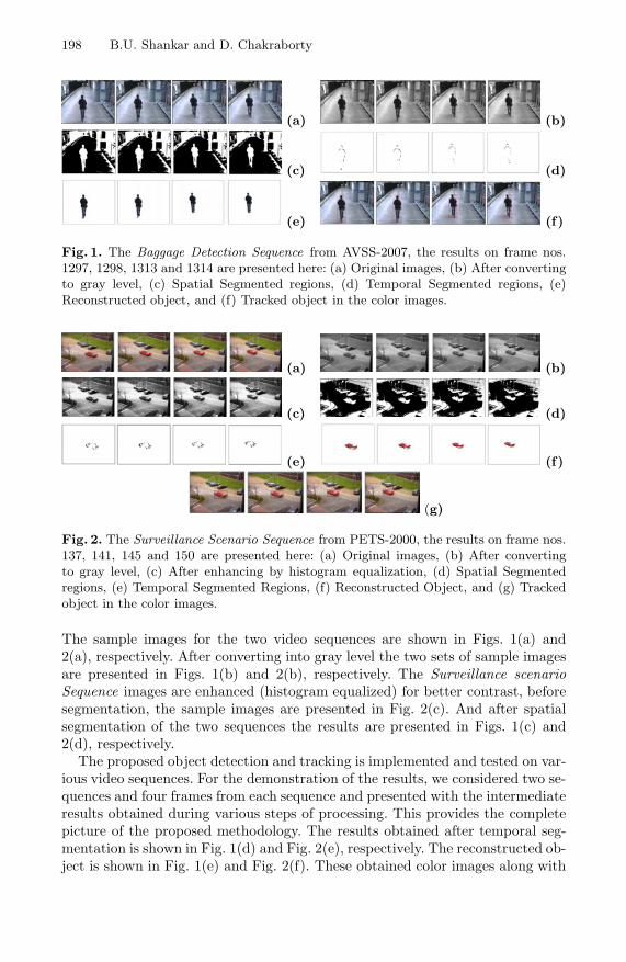
198 B.U. Shankar and D. Chakraborty
(a) (b)
(c) (d)
(e) (f)
Fig. 1. The Baggage Detection Sequence from AVSS-2007, the results on frame nos.1297, 1298, 1313 and 1314 are presented here: (a) Original images, (b) After convertingto gray level, (c) Spatial Segmented regions, (d) Temporal Segmented regions, (e)Reconstructed object, and (f) Tracked object in the color images.
(a) (b)
(c) (d)
(e) (f)
(g)
Fig. 2. The Surveillance Scenario Sequence from PETS-2000, the results on frame nos.137, 141, 145 and 150 are presented here: (a) Original images, (b) After convertingto gray level, (c) After enhancing by histogram equalization, (d) Spatial Segmentedregions, (e) Temporal Segmented Regions, (f) Reconstructed Object, and (g) Trackedobject in the color images.
The sample images for the two video sequences are shown in Figs. 1(a) and2(a), respectively. After converting into gray level the two sets of sample imagesare presented in Figs. 1(b) and 2(b), respectively. The Surveillance scenarioSequence images are enhanced (histogram equalized) for better contrast, beforesegmentation, the sample images are presented in Fig. 2(c). And after spatialsegmentation of the two sequences the results are presented in Figs. 1(c) and2(d), respectively.
The proposed object detection and tracking is implemented and tested on var-ious video sequences. For the demonstration of the results, we considered two se-quences and four frames from each sequence and presented with the intermediateresults obtained during various steps of processing. This provides the completepicture of the proposed methodology. The results obtained after temporal seg-mentation is shown in Fig. 1(d) and Fig. 2(e), respectively. The reconstructed ob-ject is shown in Fig. 1(e) and Fig. 2(f). These obtained color images along with

Spatiotemporal Approach for Tracking Using Rough Entropy 199
the tracker are presented in the Figs. 1(f) and 2(g), respectively, for the two se-quences. From the demonstrated results it can be seen that the moving objects aredetected and tracked properly. The enhancement has helped in detection of object(car) accurately, in Fig. 2. However in the Baggage Detection Sequence the avail-able contrast was sufficient to detect the moving person properly. We comparedwith another thresholding based method and found to be performing better, butresults can not be presented here due to limitation on length of the paper.
5 Conclusions
Here we have proposed rough entropy and frame difference based spatiotemporalsegmentation for object detection and tracking in a video sequence. We proposeda method of image granulation using quad-tree decomposition and a modifica-tion in the rough entropy function for object and background segmentation andthen combined it with the results obtained after frame subtraction based tem-poral segmentation to reconstruct the moving object in the video sequence. Therough entropy based thresholding in window around the threshold detected inthe previous frame makes it efficient. The proposed method has been tested onvarious video sequences, and the initial experimental results are very satisfying.The proposed method uses spatial as well as temporal information and gives anaccurate and efficient algorithm.
References
1. AVSS-2007: Fourth IEEE Int. Conf. Adv. Video & Signal Based Surveillance (2007)2. Butenkov, S.A.: Granular computing in image processing and understanding. In:
Proc. IASTED Int. Conf. Artificial Intelligence and Applns, pp. 811–816 (2004)3. Chakraborty, D., Shankar, B.U.: Rough entropy based object segmenatation and
tracking in video images. Tech. Rep. MIU/TR/-02/10, MIU, ISI (2010)4. Hassanien, A.E., et al.: Rough sets and near sets in medical imaging: A review.
IEEE Trans. on Information Technology in Biomedicine 13(6), 955–968 (2008)5. Maggio, E., Cavallaro, A.: Video Tracking - Theory and Practice. Wiley, Chichester
(2010)6. Pal, S.K., Peters, J.F. (eds.): Rough Fuzzy Image Analysis: Foundations and
Methodologies. Chapman & Hall/CRC (2010)7. Pal, S.K., Uma Shankar, B., Mitra, P.: Granular computing, rough entropy and
object extraction. Pattern Recognition Letters 26(16), 2509–2517 (2005)8. Pawlak, Z.: Rough Sets: Theoretical Aspects of Reasoning about Data. Kluwer
Academic Publishers, Norwell (1992)9. PETS-2000: IEEE Int. WS Perfor. Evaluation of Tracking and Surveillance (2000)
10. Pratt, W.K.: Digital Image Processing. John Wiley & Sons, New York (1991)11. Tekalp, A.M.: Digital Video Processing. Prentice Hall, New Jersey (1995)12. Shankar, B.U.: Novel classification and segmentation techniques with application
to remotely sensed images. In: Peters, J.F., Skowron, A., Marek, V.W., Orlowska,E., Slowinski, R., Ziarko, W.P. (eds.) Transactions on Rough Sets VII. LNCS,vol. 4400, pp. 295–380. Springer, Heidelberg (2007)
13. Yilmaz, A., Javed, O., Shah, M.: Object tracking: A survey. ACM ComputingSurveys 38(4), 1264–1291 (2006)
OSiMa: Human Pose Estimation from a Single
Image
Nipun Pande and Prithwijit Guha
TCS Innovation Labs, New Delhinipun.pande,[email protected]
Abstract. Human upper body pose estimation plays a key role in appli-cations related to human-computer interactions. We propose to developan avatar based video conferencing system where a user’s avatar is ani-mated following his/her gestures. Tracking gestures calls for human poseestimation through image based measurements. Our work is motivatedby the pictorial structures approach and we use a 2D model as a col-lection of rectangular body parts. Stochastic search iterations are usedto estimate the angles between these body parts through OrientationSimilarity Maximization (OSiMa) along the outline of the body model.The proposed approach is validated on human upper body images withvarying levels of background clutter and has shown (near) accurate poseestimation results in real time.
1 Introduction
Human pose estimation through visual sensing has potential applications in thefields of human computer interfaces and motion capture for realistic 3D ani-mations, biomechanical analysis, robot control and visual surveillance (activityrecognition). Our work is aimed at developing an avatar based video conferenc-ing system where a user’s avatar in a virtual meeting room is animated followinghis/her gestures. Here, we present a part of this work where we restrict ourselvesto the pose estimation of human upper body only while assuming a single personin the view. Tracking human poses through image based measurements has twomajor sub-divisions – first, the (near) accurate estimation of the human posefrom the very first image and second, re-estimation of the pose from the sub-sequent images using the previous instant’s pose as a prior. Here, we focus onthe necessary first step, i.e. human upper body pose estimation from a singleimage to initialize the gesture tracking procedure.
Existing literature on human body pose estimation is vast [1], most of whichassume the existence of a background model to handle the scene clutter. How-ever, we restrict our discussions to approaches aimed at retrieving human upperbody pose from single images only (i.e. no temporal information). Ramanandescribes an iterative parsing process to estimate the pose using region basedbody models e.g. color histogram to refine the body part positions [2]. An ap-proach following this is [3]. Here an upper body detector is used with GrabCutto determine the foreground area followed by parsing to fit a pictorial structure
S.O. Kuznetsov et al. (Eds.): PReMI 2011, LNCS 6744, pp. 200–205, 2011.c© Springer-Verlag Berlin Heidelberg 2011

OSiMa: Human Pose Estimation from a Single Image 201
model. An interesting work which takes into account natural shape and posevariations is Contour People [4]. Here segmentation of the scene into foregroundand background regions is done and a shape deformation model is trained using3D SCAPE model.[5] express a subset of model parameters as kernel regressionestimates from a learned sparse set of exemplars. An exemplar based pose repre-sentation called “poselet” is used in [6]. To detect the presence of each poselet aclassifier is trained for each poselet using standard linear SVM and the histogramof oriented gradients.
We have adopted a human body model consisting of rectangular body parts(head, torso and lower/upper arms) with circles at joints to render a smoothbody contour in the image plane. A Haar feature based frontal face detector [7]is used to localize the head in the image. The dimensions of the different bodyparts are computed from the head (or face) width using available anthropo-metric ratio data [8]. Now, considering the head position as pivot, several bodymodel outlines can be rendered by varying the angles between the body parts.This provides us with a set of straight lines on the image plane since the bodymodel is a constructed as a collection of rectangles where each body part is aset of two parallel lines e.g. the two edges of the arm or the torso. The similaritybetween the image gradient directions and the line orientation along such anedge of some body part is defined as a measure for localizing the body part. Anobjective function is defined by combining these orientation similarity measureswhich is maximized through stochastic search iterations [9]. Existing approacheshave employed color constancy assumptions, limb detectors along with bodypart connectivity constrained maximization for pose estimation [2,10,3]. Thus,these approaches are heavily dependent on clothing color constancy, hand skinexposure and are far from real time execution. On the other hand, we have usedonly the face detector and localized the body parts using image gradient mea-surements (and hence independent of color constancy assumptions) one by onethereby reducing the dimensionality of the domain of stochastic search leadingto real time performance (Section 2). The proposed approach is experimentallyvalidated on a number of human upper body images containing varying levelsof background clutter (Section 3). Finally, we conclude in Section 4 and outlinethe future extensions.
2 Upper Body Pose Estimation
Figure 1 shows the 2D human body model (with body part dimensions and jointangles) used in our work. We assume the human body to be near vertical for ourparticular application domain and hence assume the joint angle between torsoand the vertical axis of the head (θt) to lie in the interval [− π
12, π
12]. The joint
angles made by the left (θlua) and right (θrua) upper arms with the torso axis areassumed to vary in the interval of [0, π]. However, considering the possibilities ofroll in the upper arms, the angles between the lower and upper arms at left (θle)and right (θre) elbows are assumed to lie in the interval of [π
4, 7π
4]. The image
co-ordinates of the joints viz. Jth (between head and torso), Jtl (between torso
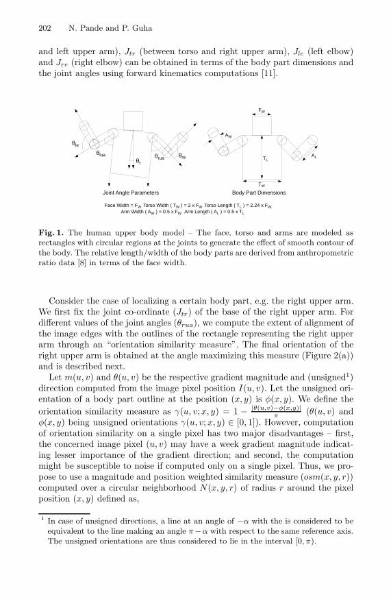
202 N. Pande and P. Guha
and left upper arm), Jtr (between torso and right upper arm), Jle (left elbow)and Jre (right elbow) can be obtained in terms of the body part dimensions andthe joint angles using forward kinematics computations [11].
Fig. 1. The human upper body model – The face, torso and arms are modeled asrectangles with circular regions at the joints to generate the effect of smooth contour ofthe body. The relative length/width of the body parts are derived from anthropometricratio data [8] in terms of the face width.
Consider the case of localizing a certain body part, e.g. the right upper arm.We first fix the joint co-ordinate (Jtr) of the base of the right upper arm. Fordifferent values of the joint angles (θrua), we compute the extent of alignment ofthe image edges with the outlines of the rectangle representing the right upperarm through an “orientation similarity measure”. The final orientation of theright upper arm is obtained at the angle maximizing this measure (Figure 2(a))and is described next.
Let m(u, v) and θ(u, v) be the respective gradient magnitude and (unsigned1)direction computed from the image pixel position I(u, v). Let the unsigned ori-entation of a body part outline at the position (x, y) is φ(x, y). We define theorientation similarity measure as γ(u, v;x, y) = 1 − |θ(u,v)−φ(x,y)|
π(θ(u, v) and
φ(x, y) being unsigned orientations γ(u, v; x, y) ∈ [0, 1]). However, computationof orientation similarity on a single pixel has two major disadvantages – first,the concerned image pixel (u, v) may have a week gradient magnitude indicat-ing lesser importance of the gradient direction; and second, the computationmight be susceptible to noise if computed only on a single pixel. Thus, we pro-pose to use a magnitude and position weighted similarity measure (osm(x, y, r))computed over a circular neighborhood N(x, y, r) of radius r around the pixelposition (x, y) defined as,
1 In case of unsigned directions, a line at an angle of −α with the is considered to beequivalent to the line making an angle π−α with respect to the same reference axis.The unsigned orientations are thus considered to lie in the interval [0, π).
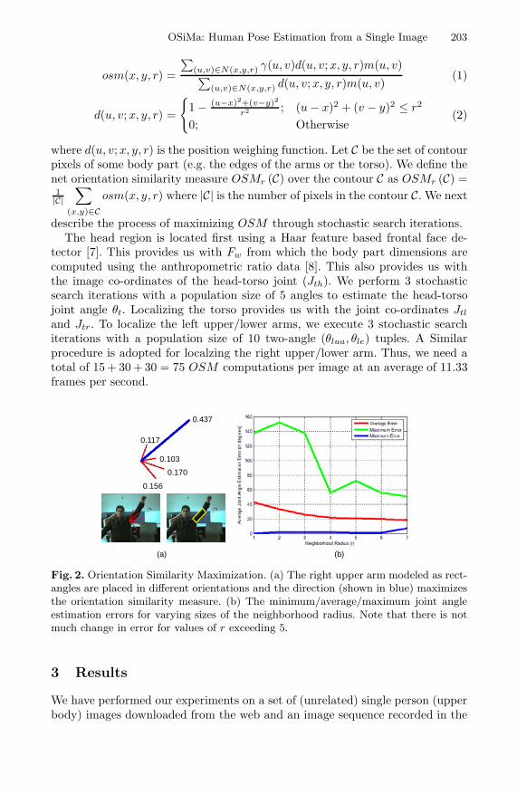
OSiMa: Human Pose Estimation from a Single Image 203
osm(x, y, r) =
∑(u,v)∈N(x,y,r) γ(u, v)d(u, v;x, y, r)m(u, v)∑
(u,v)∈N(x,y,r) d(u, v;x, y, r)m(u, v)(1)
d(u, v;x, y, r) =
1 − (u−x)2+(v−y)2
r2 ; (u − x)2 + (v − y)2 ≤ r2
0; Otherwise(2)
where d(u, v;x, y, r) is the position weighing function. Let C be the set of contourpixels of some body part (e.g. the edges of the arms or the torso). We define thenet orientation similarity measure OSMr (C) over the contour C as OSMr (C) =1|C|
∑
(x,y)∈Cosm(x, y, r) where |C| is the number of pixels in the contour C. We next
describe the process of maximizing OSM through stochastic search iterations.The head region is located first using a Haar feature based frontal face de-
tector [7]. This provides us with Fw from which the body part dimensions arecomputed using the anthropometric ratio data [8]. This also provides us withthe image co-ordinates of the head-torso joint (Jth). We perform 3 stochasticsearch iterations with a population size of 5 angles to estimate the head-torsojoint angle θt. Localizing the torso provides us with the joint co-ordinates Jtl
and Jtr. To localize the left upper/lower arms, we execute 3 stochastic searchiterations with a population size of 10 two-angle (θlua, θle) tuples. A Similarprocedure is adopted for localzing the right upper/lower arm. Thus, we need atotal of 15 + 30 + 30 = 75 OSM computations per image at an average of 11.33frames per second.
Fig. 2. Orientation Similarity Maximization. (a) The right upper arm modeled as rect-angles are placed in different orientations and the direction (shown in blue) maximizesthe orientation similarity measure. (b) The minimum/average/maximum joint angleestimation errors for varying sizes of the neighborhood radius. Note that there is notmuch change in error for values of r exceeding 5.
3 Results
We have performed our experiments on a set of (unrelated) single person (upperbody) images downloaded from the web and an image sequence recorded in the

204 N. Pande and P. Guha
laboratory settings with varying levels of background clutter. A set of 20 imagesfrom this data set are ground truthed through manual measurement of the jointangles. We note that the accuracy of pose estimation directly depends on theneighborhood radius r in the computation of OSM . For a certain value of r,we compute the average joint angle estimation error over 5 joint angles from20 images. Figure 2(b) shows the maximum, average and minimum estimationerrors for 1 ≤ r ≤ 7. Significant changes in the error is not observed for r > 5.However, higher values of r lead to larger number of computations and hence wefix r = 5 for our experiments. The results of human upper body pose estimationon 12 images from the data set are shown in figure 3.
(a) (b) (c) (d)
(e) (f) (g) (h)
(i) (j) (k) (l)
Fig. 3. Experimental results performed on a set of human upper body images withvarying levels of background clutter. Although the joint angles are estimated accurately,the human body outline is not fitted tightly on some cases on account of person toperson variations in anthropometric data and loose clothing. Failures in localizing inright lower arm is observed in (b) due to loose clothing and strong background clutter(red pipe); where as in (d) the reason is the deviation from the average anthropometricratio data.
4 Conclusion
We have presented a methodology for human upper body pose estimation froma single image using a 2D model (motivated by pictorial structures approach).We have defined an orientation similarity measure to align the body parts (torsoand arms) in images. A Haar feature based frontal face detection followed bystochastic search iterations are used to localize the body parts while maximizing
OSiMa: Human Pose Estimation from a Single Image 205
the proposed orientation similarity measure computed along the outlines of thebody parts. In contrast to the existing works in human pose estimation fromsingle images, we have achieved high accuracy while performing in real time.
The current work has only focused on the pose estimation from a single imageand is a necessary first step towards tracking the pose of the user. We identifythe future extensions in two directions. First, the current work is to be extendedto tracking where the stochastic search space is further reduced using temporalinformation. However, it is still not fully possible to estimate the accurate 3Dpose from single view information. The second possible extension will be in thedirection of combining the image based orientation similarity measurements withdepth data obtained from range sensors to avail accurate 3D pose.
References
1. Moeslund, T., Hilton, A., Kruger, V.: A survey of advances in vision-based humanmotion capture and analysis. Computer Vision and Image Understanding 104, 90–126 (2006)
2. Ramanan, D.: Learning to parse images of articulated bodies. In: Neural Informa-tion Processing Systems (NIPS), pp. 1129–1136 (2006)
3. Ferrari, V., Marin-Jimenez, M., Zisserman, A.: Pose search: Retrieving people usingtheir pose. In: IEEE Conference on Computer Vision and Pattern Recognition, pp.1–8 (2009)
4. Freifeld, O., Weiss, A., Zuf, S., Black, M.J.: Contour people: A parameterized modelof 2d articulated human shape. In: IEEE Conference Computer Vision and PatternRecognition, pp. 639–646 (2010)
5. Sapp, B., Jordan, C., Taskar, B.: Adaptive pose priors for pictorial structures. In:IEEE Conference Computer Vision and Pattern Recognition, pp. 422–429 (2010)
6. Yang, W., Wang, Y., Mori, G.: Recognizing human actions from still images withlatent poses. In: IEEE International Conference on Computer Vision and PatternRecognition, pp. 2030–2037 (2010)
7. Viola, P., Jones, M.: Robust real-time face detection. International Journal onComputer Vision 57, 137–154 (2004)
8. NASA: Anthropometric Source Book, vol. 2. Springfield VA (1978)9. Spall, J.C.: Introduction to Stochastic Search and Optimization: Estimation, Sim-
ulation and Control. Wiley-Interscience, Hoboken (2003)10. Ferrari, V., Marin-Jimenez, M., Zisserman, A.: Progressive search space reduction
for human pose estimation. In: IEEE Conference on Computer Vision and PatternRecognition, pp. 1–8 (2008)
11. Craig, J.J.: Introduction to Robotics Mechanics and Control. Pearson EducationInc., London (2003)

Scene Categorization Using Topic Model Based
Hierarchical Conditional Random Fields
Vikram Garg, Ehtesham Hassan, Santanu Chaudhury, and M. Gopal
Department of Electrical Engineering, IIT Delhi, [email protected], [email protected],[email protected], [email protected]
Abstract. We propose a novel hierarchical framework for scene catego-rization. The scene representation is defined by latent topics extracted byLatent Dirichlet Allocation. The interaction of these topics across scenecategories is learned by probabilistic graphical modelling. We use Condi-tional Random Fields in a hierarchical setting for discovering the globalcontext of these topics. The learned random fields are further used forcategorization of a new scene. The experimental results of the proposedframework is presented on standard datasets and on image collectionobtained from the internet.
Keywords: Scene categorization, Latent dirichlet allocation, Conditionalrandom fields.
1 Introduction
In this paper we propose a novel hierarchical framework for scene categoriza-tion. The framework utilizes the latent concept information for scene categoriza-tion. The concept extraction is performed by latent topic modelling at the localpatch level. For similar scenes, the organization of these topics represents sim-ilar graphical structure. We learn the graphical structure of these topics acrossvarious scene categories through a probabilistic graphical model. The frameworkrecognizes a new scene based on the learned graphical structures.
The natural scene categorization is a widely researched problem in contentbased image retrieval. The fundamental problem here lies in identifying differ-ent objects and understanding their interaction for scene definition. However,the object extraction in a natural scene requires robust segmentation algorithm.Topic modelling based methods provide efficient solution to this problem. Thesemethods represent the image through mixture of latent topics. The topic as-signment effectively performs the semantic image segmentation in feature space.In the related works, Yamaguchi and Maruyama have used topic distributionbased image representation for image classification [4]. The topic modelling isperformed by Probabilistic Latent Semantic Analysis using the SIFT key pointsbased bag-of-words model. In another work, Ergul and Arica perform the pLSAbased topic analysis of the image at multiple scales [5]. The topic modelling by
S.O. Kuznetsov et al. (Eds.): PReMI 2011, LNCS 6744, pp. 206–212, 2011.c© Springer-Verlag Berlin Heidelberg 2011

Scene Categorization Using Topic Model 207
PLSA shows biased topic assignment towards training images. The LDA incor-porates the document distribution for topic learning and provides robust topicmodelling framework. [7] have learned a LDA based hierarchical model for imagecategorization while [11] have employed a generative hierarchical LDA model forunsupervised discovery of topic hierarchies in visual objects. The recent workWang et al. have applied supervised LDA for discovering the latent topics [13].The contextual relationship between the topics is important semantic informa-tion for scene categorization. [12] has used a generative Bayesian network toutilize the position and expected appearance of object parts while in the presentwork, we propose a novel scene categorization framework by exploiting the topiclevel contextual relationship in a natural image. The framework extracts thelocal patch level topics in scene using LDA. The probabilistic graphical modelsexhibit excellent capability to learn the sequential data. The recent works haveextensively applied Conditional Random Fields (CRFs) based graphical modelfor Image classification [9][10][13]. However discovering the contextual relation-ship between the topics by CRFs is not yet explored. Our work presents a novelapproach in this direction by applying hierarchical CRF to discover the topicbased global context for scene recognition.
The organization of the paper is as follows: The section 2 presents scenerepresentation patch level topic modelling of the image. The section 3 presentsthe proposed framework for scene categorization. The section 4 presents theexperimental results. Finally we conclude and present perspective of our work.
2 Feature Based Image Representation Using LDA
The visual content representation forms important step for a scene understand-ing. The bag-of-words model has been the preferred approach for natural imagerepresentation. Using the model, image representation is defined as the distribu-tion of local features properties. The SIFT based descriptor provide an efficientapproach to extract the local image features [1]. The descriptor is computedas set of local orientation histograms centred at key-points obtained by multi-scale analysis of the image. The SIFT descriptor extracts dense points at theboundaries, and image segments having sharp changes. Whereas the smoothsegments are represented by sparse key points. The bag-of-words model in thiscase represents the image by a biased representation leaving significant amountof visual information unutilized. For example, a landscape scene having sky treeand building will get biased distribution of key-points near tree and building.Therefore we follow grid based approach for extracting the local image features.The approach covers all the segment of the image and assigns uniform weightto all the segments. Using the image patches in the grid, bag-of-words model isgenerated. The bag-of-words representation is used to generate the image repre-sentation by discovering the latent topics in a scene. The topics here representthe semantic entity which defines the distribution of various image patches inthe latent space. The Latent Dirichlet allocation is applied to extract the topicdistribution over the scene image collection. The LDA is defined as a genera-tive probabilistic model for collections of documents [2]. In the context of topic
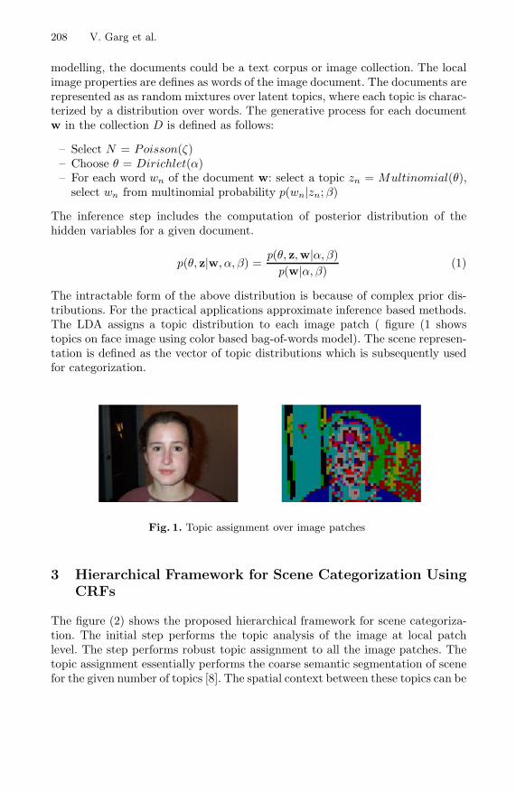
208 V. Garg et al.
modelling, the documents could be a text corpus or image collection. The localimage properties are defines as words of the image document. The documents arerepresented as as random mixtures over latent topics, where each topic is charac-terized by a distribution over words. The generative process for each documentw in the collection D is defined as follows:
– Select N = Poisson(ζ)– Choose θ = Dirichlet(α)– For each word wn of the document w: select a topic zn = Multinomial(θ),
select wn from multinomial probability p(wn|zn; β)
The inference step includes the computation of posterior distribution of thehidden variables for a given document.
p(θ, z|w, α, β) =p(θ, z,w|α, β)
p(w|α, β)(1)
The intractable form of the above distribution is because of complex prior dis-tributions. For the practical applications approximate inference based methods.The LDA assigns a topic distribution to each image patch ( figure (1 showstopics on face image using color based bag-of-words model). The scene represen-tation is defined as the vector of topic distributions which is subsequently usedfor categorization.
Fig. 1. Topic assignment over image patches
3 Hierarchical Framework for Scene Categorization UsingCRFs
The figure (2) shows the proposed hierarchical framework for scene categoriza-tion. The initial step performs the topic analysis of the image at local patchlevel. The step performs robust topic assignment to all the image patches. Thetopic assignment essentially performs the coarse semantic segmentation of scenefor the given number of topics [8]. The spatial context between these topics can be

Scene Categorization Using Topic Model 209
efficiently learned by a probabilistic graphical model. The CRFs are an efficienttool for such problems. However, the long range contextual dependencies inthe semantic segmentation cannot be captured by a simple graphical model.Therefore, we introduce category specific graphical model (CRFs). We traincategory specific CRFs using the patch-ground-truth, and assign semantic labelsover the latent topics. The exact notion of the category specific CRFs is thesmoothening of latent topics by supervised learning. The top level CRFs learnsthe structure of the contextual graph belonging to each category of images.
The CRFs is a discriminative modelling tool for segmenting and labelling thesequential data [3]. The CRFs work under the maximum entropy principle andobserve the features as sequence data. Consider X the random variable over datasequences to be labelled and Y the random variable for the corresponding labelsequences. Using the fundamental theorem of random fields, joint distributionover the label sequence Y given X is defined as
pθ(y|x) ∝ exp(∑
e∈E,k
λkfk(e, y|v, x) +∑
v∈V,k
μkgk(v, y|e, x)) (2)
V and E represent the vertices and edges of graph G, such that label sequence Yis indexed by the vertices of G. Here x represents a data sequence, y representsa label sequence, and y|S is set of components of y associated with the verticesin sub-graph S. The function fk defines the input dependent evidences and gk
gk represents the pair-wise coupling labels of sequence data. The parameterestimation problem determines the parameters θ = (λ1, μ1, λ2, μ2, ...) by themaximization of log-likelihood objective as
O(θ) =N∑
i=1
log pθ(yi|xi) ∝∑
x,y
p(x, y)log pθ(y|x) (3)
For category specific CRFs, graph G is represented by function fk as thelikelihood of image patch having ith topic and function gk represents smoothnessprior to encourage the neighbouring image patches to obtain same label. Functionfk has the form as fk(e, y|v, x) = xkδ(y, lk), δ is the Kronecker delta and krepresents the indices of parameter set from θ and lk is the label of the patch forkth parameter set. The smoothness prior gk is defined as δ(y1, lk)δ(y2, lk). It isclear that the smoothness prior is independent of patch features. The top levelCRF learns the graphical structure of latent topics for image collection usingthe sequence of semantic labels assigned from first level CRFs.
A new image is categorized by topic assignment using patch level imagefeatures. The topic level representation of the image is supplied to the entirecategory specific CRFs. For N scene categories, the top level CRF receives Nsemantic graphs for the new image. For each semantic graph, the top level CRFassigns marginal probability distribution. The final category assignment for thenew scene is done as the label corresponding to maximum marginal probabilityfor all the semantic graphs.

210 V. Garg et al.
Fig. 2. Hierarchical framework for scene categorization
4 Experimental Results and Discussion
We have evaluated the proposed framework on standard MSRC dataset1, Cal-tech 101 dataset2 and image collection from internet. The MSRC dataset isapplied for training our system as the dataset contains pixel level ground-truth.The pixel-level ground truth is converted to patch-level by majority voting. Thetraining set consists of 30 randomly selected corresponding to 9 super categoriesBicycle, Building, Car, Cattle, Cow, Face, Sheep, Plane, and Tree. The im-age set (270 images) have been normalized to 105X154. The images patches aredetected by overlaying a grid of 15 × 22, therefore giving 330 patches of 7X7.The bag-of-words model is generated by clustering the image patches from 5randomly selected training images corresponding to each category. The topicassignment over complete set of image patches is done by learning a LDA for 10semantic concepts. We use topic modelling toolbox provided by Steyers and Grif-fiths [14] for topic modelling. The probabilistic graphical modelling is performedby CRF implementation provided by Sarawagi [15]. Initially the framework hasbeen tested for the same set of training images. We have compared our resultswith the best case accuracy preseted in [8] in table 1. The second evaluation theproposed framework is performed using the Caltech 101 dataset images. The ex-periment evaluates the proposed framework for unseen images belonging to twocategories. The experiment evaluates the robustness of the proposed frameworkas the dataset is primarily prepared for object recognition problem. The ex-periment is performed by randomly selecting 30 images corresponding to Plane
1 http://research.microsoft.com/en-us/projects/objectclassrecognition/2 http://www.vision.caltech.edu/Image Datasets/Caltech101/

Scene Categorization Using Topic Model 211
Table 1. Recognition accuracy for training image set
Category Bicycle Building Car Cattle Cow Face Sheep Plane Tree Average
Presented Acc. 90 96 93 90 93 96 96 96 96 94
Best Average Acc. [8] 94 77 73 N.A. 86 99 N.A. 73 71 82
*categories with N.A. were not availabe in [8].
Table 2. Recognition accuracy for image set from Caltech dataset
Category Plane Face
Accuracy 67 45
Tree Tree Tree Sheep Plane Plane
Plane Plane Plane Cow Cattle Sheep
Building Cow Cow Face Face Face
Face Bicycle Plane Building Sheep Car
Car Sheep Sheep Cow Sheep Cow
Fig. 3. Evaluation Images and assigned category
and 30 images corresponding to Face category. The results are presented in thetable 2. The third evaluation of the proposed framework is performed on imagecollection obtained from internet. The collection contains 30 images belongingto 6 training categories. The average accuracy of 60% is achieved. The imagewith their final category assignment are shown in the figure 3. The results (figure3) establish the robustness of the proposed framework as testing images belongto variety of domains. The category assignment for these images can be easily
212 V. Garg et al.
verified by close observation. The results show that our framework efficientlyutilizes semantic information of the scene for categorization.
5 Conclusion
A novel framework for scene categorization is presented. The patch level latenttopics extracted by LDA have been used for scene representation. A novel appli-cation of hierarchical CRFs is demonstrated for scene recognition. The two-layerCRFs performs topic level smoothening at first layer and subsequently performthe scene recognition by learning the spatial context of different topics. The ex-perimental evaluation on standard dataset and images obtained from the internetvalidate the efficiency and robustness of the proposed framework.
References
1. Lowe, D.G.: Object recognition from local scale-invariant features. In: Proceedingsof the International Conference on Computer Vision, vol. 2, pp. 1150–1157 (2000)
2. Blei, D.M., Ng, A.Y., Jordan, M.I.: Latent Dirichlet allocation. Journal of MachineLearning Research, 993–1022 (2003)
3. Lafferty, J., McCallum, A., Pereira, F.: Conditional random fields: Probabilisticmodels for segmenting and labelling sequence data. In: Proceedings of the Inter-national Conference on Machine Learning, pp. 282–289. Morgan Kaufmann, SanFrancisco (2001)
4. Yamaguchi, T., Maruyama, M.: Image categorization by a classifier based on prob-abilistic topic model. Pattern Recognition (2008)
5. Ergul, E., Arica, N.: Scene Classification Using Spatial Pyramid of Latent Topics.In: International Conference on Pattern Recognition (2010)
6. Fei, L.F., Persona, P.: A Bayesian Hierarchical Model for Learning Natural SceneCategories. In: IEEE Conference on Computer Vision and Pattern Recognition(2005)
7. Wang, C., Blei, D., Fei, L.F.: Simultaneous Image Classification and Annotation.In: IEEE Conference on Computer Vision and Pattern Recognition (2009)
8. Passino, G., Patras, I., Izquierdo, E.: Latent Semantic Local Distribution for CRF-based Image Semantic Segmentation. In: British Machine Vision Conference (2009)
9. Zhong, P., Wang, R.: Learning Conditional Random Fields for Classification ofHyperspectral Images. In: IEEE Transactions on Image Processing (2010)
10. Wang, X., Liu, X., Shi, Z., Shi, Z., Sui, H.: Voting Conditional Random Fields forMulti-label Image Classification. In: International Congress on Image and SignalProcessing (2010)
11. Sivic, J., Russell, B.C., Zisserman, A., Freeman, W.T., Efros, A.A.: Unsuperviseddiscovery of visual object class hierarchies. In: Computer Vision and Pattern Recog-nition (2008)
12. Sudderth, E.B., Torralba, A., Freeman, W.T., Willsky, A.S.: Learning Hierarchi-cal Models of Scenes, Objects, and Parts. In: IEEE International Conference onComputer Vision (2005)
13. Wang, Y., Gong, S.: Conditional Random Field for Natural Scene Categorization.In: British Machine Vision Conference (2007)
14. Steyvers, M., Griffiths, T.: Matlab Topic Modelling Toolbox Version 1.3.215. Sarawagi, S.: CRF package, http://crf.sourceforge.net/

Uncalibrated Camera Based Interactive 3DTV
M.S. Venkatesh, Santanu Chaudhury, and Brejesh Lall
Department of Electrical Engineering, IIT Delhi, [email protected], [email protected], [email protected]
Abstract. In this paper we propose a novel architecture for an interac-tive 3DTV system based on multiple uncalibrated cameras placed at gen-eral positions. The signal representation scheme proposed is compatiblewith the standard multi view coding framework making it amenable tousing existing coding and compression algorithms. The proposed schemealso fits naturally to the concept of true 3DTV viewing experience wherethe viewer can choose a novel viewpoint based on the contents of thescene.
Keywords: Interactive 3DTV, Uncalibrated cameras, Plane sweeping,Depth map.
1 Introduction
In this paper we propose a novel architecture for interactive 3DTV which enablesa viewer to choose a 3D view of the scene based on scene content. We assumethat the scene is captured by multiple uncalibrated cameras in general positions.We use a statistical learning method to automatically detect scene constraintsthat are then used to calibrate the cameras as well as provide orientation in-formation to generate depth maps for each view. The advantage of our signalrepresentation scheme is that it is compatible with the standard Multi ViewCoding framework of video plus depth[3,4]. This enables the direct applicationof the existing coding and compression algorithms. The scene orientation infor-mation can be easily embedded in the meta-data part of the signal. The noveltyof our architecture is that the scene orientation information allows the user toselect different viewpoints based on the scene content to interactively generatenovel 3D views at the receiver’s end. Typical applications of our methodologyis in 3D viewing of outdoor scenes like monuments, urban buildings etc. Theuser can interactively specify which part of the monument he wants to view in3D. The typical characteristics of such scenes like orthogonal planes assist inautomatic detection of scene constraints and orientations.
3DTV is considered as the next step in enhancing the user viewing experience.A true 3DTV is supposed to give a 3D view of the scene as well allow the userto choose different viewpoints of the scene. Our approach fits naturally in thiscontext. The video plus depth format [3] in which each video is accompanied bya per pixel depth data is considered most suitable for generation of high quality3D views as well as intermediate view synthesis at the receiver. To generate
S.O. Kuznetsov et al. (Eds.): PReMI 2011, LNCS 6744, pp. 213–219, 2011.c© Springer-Verlag Berlin Heidelberg 2011

214 M.S. Venkatesh, S. Chaudhury, and B. Lall
the depth map, camera calibration information is required. Camera calibrationfrom scene constraints and generation of depth maps from stereo and multi viewimages are topics that have been extensively studied in computer vision [15]. Inour methodology we automatically discover these scene constraints and exploitthem for the calibration of the cameras. Plane sweeping algorithms like [5,6,7]outperform standard stereo matching algorithms for generation of depth map inpresence of oblique structures in scenes. The directions along which the planesare swept are determined by analysis of a sparse or dense set of 3D points. Inour approach, the scene classification step itself gives us the orientations used forplane sweeping. The dense depth map thus generated is then used to generateexisting as well as interpolate novel stereo views of the scene without performingan explicit 3D reconstruction using a Depth Image Based Rendering technique[4]. These novel views are specified by new camera viewpoints with respect tothe existing viewpoints.
Some work has been done regarding user interaction in 3DTV [12]. The au-thors in [13] allow for view switching, frozen moment and view sweeping at thereceiver end. The novelty of our approach is that it allows the user to choose theviewpoint based on scene content to be able to view novel 3D views of parts ofthe scene as well as arbitrary novel views of the complete scene. Automaticallyextracting the scene constraints and orientations from the images to use them forcamera calibration is also a novelty of our work. Another novelty of our methodis that we obtain the direction of family of planes and the confidence measuresfrom the scene classification [1] step itself.
In section 2, we present the basic outline of our system architecture. Section 3outlines the novel view viewpoint selection and the DIBR technique used to syn-thesize novel views. In section 4 we present experimental results and discussionsfollowed by the conclusion and future work.
2 System Architecture
We illustrate our proposed methodology with an example of a building as shownin the figure 1. Images are taken from multiple uncalibrated cameras placed atgeneral positions. Then classifier of [1] is used to classify the image and identifythe horizontal(green) and vertical (red) planes. This constraint is then used tocalibrated the cameras. The orientations of scene (indicated by arrows) are alsorecovered along with their confidence measures. This is used to generate a depthmap. The orientation information along with the video plus depth forms thesignal representation. At the receiver end the user interactively chooses certainparts of the scene to view and then the orientation information in that part ofthe image is used to obtain the novel 3D views of the scene.
2.1 Scene Classification
The authors in [1] classify the outdoor scene into geometric classes that de-pend on the orientation of the particular object in the scene based on statistical

Uncalibrated Camera Based Interactive 3DTV 215
Fig. 1. Outline of the proposed architecture
learning. They classify an image into planar vertical regions (facing left, center,or right), ground (horizontal) regions, sky and non planar regions (porous andsolid) without using any calibration information. A confidence measure is alsoassociated with each class.
2.2 Camera Calibration
Many methods exist for calibrating the cameras using the scene constraints.Specifically, we use the orthogonality of the vertical and horizontal planes ob-tained from the scene classification step for calibration. We obtain automaticpoint correspondences from SIFT features 1 and filter mismatches by usingepipolar constraint 2. Using these point correspondences, we obtain a projec-tive reconstruction and then impose the constraints of the absolute quadric aswell as the scene constraints to upgrade it to a Euclidean one [15,2].
2.3 Obtaining the Dense Depth Map
We follow an approach closely related to [5]. Here every pixel is assigned a labelwhich indicates which plane it belongs to and an energy function which penal-izes abrupt changes in surface normals is minimized [8,9,10,11]. The confidencemeasures obtained in the scene classification step is incorporated into the costfunction.1 http://www.vlfeat.org/2 http://www.csse.uwa.edu.au/~pk/research/matlabfns/

216 M.S. Venkatesh, S. Chaudhury, and B. Lall
The normal to the planes (vertical planes and ground plane) are used todefine “k” families of parallel planes Πki given by nT
k X + dki = 0 where dki ∈[dmin, dmax]k The range [dmin, dmax] for each of the plane families are obtainedempirically. For each of the planes we find the 3x3 homography induced betweentwo images r and s [15].
This homography is used to warp the other images onto an image Ir for whomdepth map is to be generated. Then for warped image Iw, we obtain a cost forevery pixel (x, y) in the image Ir, for each of the planes Πki as
cost(x, y, Πki) =∑
(p,q)∈N
|I(x − p, y − q) − Iw(x − p, y − q)| − w ∗ log(F (Πki))
where w is a weight factor determined by experiments and F (Πki) is the prob-ability that the pixel belongs to the kith plane obtained from the confidencemeasures generated after the scene classification step. N is defined neighbour-hood of the pixel taken to be 3x3.
We formulate an energy function similar to [5] and we find out the depthZ(x, y) of each pixel (x, y) of image Ir. The depth map thus obtained is used invirtual view synthesis which is explained in the next section.
3 Virtual View Synthesis
A new virtual camera is defined by its camera parameters Rv, Kv, and Cv [15].Given an image Ir whose camera parameters are Rr, Kr and Cr and its corre-sponding depth map Zr, The image Iv is generated by [4]
The resulting virtual views have holes which are the results of either erroneousdepth values or due to truncation of the pixel positions. To fill these holes, thehomography corresponding to the nearest non zero plane label is computed andusing it, the pixel value is transferred from the given image.
3.1 Interactively Choosing the Viewpoint
The user interactively selects a part of the scene through an interface like amouse pointer or remote. For instance if a wall is selected, the virtual camerahas to be placed such the wall is fronto parallel. The orientation of this partof the image obtained after scene classification gives the direction in which thecamera has to be rotated. Once the direction is determined, the following stepsare followed.
1. A rotation matrix R′ is obtained by choosing an angle θ bounded by theangle between the normal to the plane (wall) and normal to the principalplane of the camera and a small translation t′ is chosen such that the virtualcamera undergoes a little translation so as to keep the view within the imagebounds. This Euclidean transformation is used to get the destination cameracentre Cv and rotation matrix Rv.

Uncalibrated Camera Based Interactive 3DTV 217
2. Kv is chosen to be the same as Kr. The destination camera matrixPv = KvRv[I| − Cv]
3. The new camera matrices are chosen by interpolation between the cameraPr and Pv with interpolation parameter λ ∈ [0..1] asCλ = (1 − λ)Cr + λCv
Rλ = slerp(Rr, Rv, λ)Pλ = KλRλ[I| − Cλ]where slerp refers to spherical linear interpolation.
4. To generate stereo pairs, the shift sensor algorithm [4] is used.
4 Results and Discussions
We illustrate the various steps of our proposed architecture on two standarddata sets Wadham College and Merton College.3 For Wadham College data set,we generate intermediate image sequences when the user wants to look at theleft wall. For the Merton data set we generate sequences when the user wantsto look at the right wall. Both of these sequences are generated from the imageno 2 of each data set. As the rotation increases, the rendering quality decreases.This is because of erroneous depth values and also due to mis-classification.
The average 2D re projection errors (in pixel) from the camera calibration areshown below
Data Set camera 1 camera 2 camera 3Merton College 0.410790 0.343800 0.311718Wadham College 0.405233 0.398542 0.295823
(a) (b) (c)
Fig. 2. Fig (a) shows image 2 of Wadham sequence. Fig (b) shows its scene classificationand Fig (c) is the depth map extracted.
The stereo views were generated and were displayed on a samsung 3D LEDTV. Subjective rendering quality measures were assigned based on a scale of 1to 5 in increasing order of quality. The subjective scores are shown below. Thesequences refer to the intermediate stereo views generated.
3 http://www.robots.ox.ac.uk/~vgg/data2.html

218 M.S. Venkatesh, S. Chaudhury, and B. Lall
Fig. 3. Some of the synthesized image sequences of Wadham when the user wants to“look” at the left wall
(a) (b) (c)
Fig. 4. Fig (a) shows image 2 of Merton sequence. Fig (b) shows its scene classificationand Fig (c) is the depth map extracted.
Fig. 5. Some of the synthesized image sequence of Merton when the user wants to“look” at the right wall
Fig. 6. Subjective Quality
5 Future Work and Conclusion
In this paper we have proposed a novel architecture for interactive rendering ofoutdoor scenes for 3DTV. The interactive selection of viewpoints based on scenecontent offers a different approach to novel view synthesis. We have worked with

Uncalibrated Camera Based Interactive 3DTV 219
images. The extension to videos is straight forward. As part of the future work ,we would also like to investigate the possibility of detecting objects in the sceneand allow the user to view these objects interactively. Another extension wouldbe in switching between groups of cameras and allowing the user to view objectscaptured by different groups.
Acknowledgement
This work was in part supported by the Department of Science and Technology,Govt. of India. (SR/S3/EECE/0006/2010). We would also like to thank AyeshaChaudhary for valuable feedback.
References
1. Hoeim, D., Efros, A.A., Hebert, M.: Geometrical context from a single image. In:ICCV (2005)
2. Svoboda, T., Martinec, D., Pajdla, T.: A convenient multi-camera self-calibrationfor virtual environments. PRESENCE: Teleoperators and Virtual Environ-ments 14(4), 407–422 (2005)
3. Muller, K.: View Synthesis for Advanced 3D Video Systems. EURASIP Jour-nal on Image and Video Processing 2008, article ID 438148, 11 pages (2008),doi:10.1155/2008/438148
4. Fehn, C.: A 3D-TV Approach Using Depth-Image-Based Rendering (DIBR). In:Proceedings of 3rd IASTED Conference on Visualization, Imaging, and Image Pro-cessing, September 2003, pp. 482–487 (2003)
5. Gallup, D., Frahm, J.M., Mordohai, P., Yang, Q., Pollefeys, M.: Real-Time Plane-Sweeping Stereo with Multiple Sweeping Directions. In: CVPR (2007)
6. Micusik, B., Kosecka, J.: Multi-view Superpixel Stereo in Urban Environments.International Journal of Computer Vision 89(1) (2010)
7. Sinha, S.N., Steedly, D., Szeliski, R.: Piecewise Planar Stereo for Image-based Ren-dering. In: ICCV (2009)
8. Boykov, Y., Veksler, O., Zabih, R.: Efficient Approximate Energy Minimizationvia Graph Cuts. IEEE TPAMI 23(11) (November 2001)
9. Kolmogorov, V., Zabih, R.: What Energy Functions can be Minimized via GraphCuts? IEEE TPAMI 26(2), 147–159 (2004)
10. Boykov, Y., Kolmogorov, V.: An Experimental Comparison of Min-Cut/Max-FlowAlgorithms for Energy Minimization in Vision. IEEE TPAMI 26(9), 1124–1137(2004)
11. Delong, A., Osokin, A., Isack, H.N., Boykov, Y.: Fast Approximate Energy Mini-mization with Label Costs. In: CVPR (2010)
12. Fehn, C., De La Barr, R., Pastoor, S.: Interactive 3-DTV.Concepts and Key Tech-nologies. Proceedings of IEEE 94(3) (March 2006)
13. Lou, J., Cai, H., Li, J.: A RealTime Interactive MultiView Video System. In: MM2005 Proceedings of the 13th ACM conference on Multimedia (2005)
14. Kubota, A., Smolic, A., Magnor, M., Tanimoto, M., Chen, T., Zhang, C.: MultiviewImaging and 3DTV. IEEE Signal Process. Mag. 24(6), 10–21 (2007)
15. Hartley, R., Zisserman, A.: Multiple view geometry in Computer Vision, March2004. Cambridge University Press, Cambridge (2004)

Author Identification in Bengali Literary Works
Suprabhat Das and Pabitra Mitra
Department of Computer Science and EngineeringIndian Institute of Technology Kharagpur
West Bengal, Pin - 721302, Indiasuprabhat,[email protected]
Abstract. In this paper, we study the problem of authorship identifi-cation in Bengali literary works. We considered three authors namelyRabindranath Tagore, Bankim Chandra Chattopadhyay and SukantaBhattacharyay. It was observed that simple unigram and bi-gram fea-tures along with vocabulary richness were rich enough to discriminateamongst these authors. Although results degraded slightly when train-ing set size was considerably small. For larger training set, a classificationaccuracy of above 90% for unigram feature and almost 100% for bi-gramfeature was achieved. Results could be improved further by using moresophisticated features.
Keywords: Stylometry, authorship attribution, Bengali literary works,unigram, bi-gram.
1 Introduction
Stylometry is the study of the unique linguistic styles and writing behaviors ofindividuals. Author identification is one of the important problems in stylomet-rics and it can be seen as a single-label multi-class text categorization problem.It has many academic and literary applications, like author verification, plagia-rism detection, genre classification etc. It has legal applications too, like forensiclinguistics, detection of genuine confessions. In the last few years it has success-fully been applied to broader areas, ranging from blogs, forums, wikis, email,chat and other forms of digital content to music and fine-art paintings.
Stylometry has been studied on English for long time. It was started byMendenhall [1], in the 19th century, with his work on the plays of Shake-speare. He had reported few authorship attribution method by some charac-teristic curves, based on sentence length counts and word length counts. It wasfollowed by some statistical studies by Zipf [2] and Yule [3] in the first half of 20thcentury. One of the most influential works in authorship attribution was done byMosteller and Wallace [4] on the authorship of ‘The Federalist Papers’ (a seriesof articles published in 1787-88, written by John Jay, Alexander Hamilton andJames Madison). They had employed Bayesian statistical analysis on a smallset of function words such as prepositions, conjunctions and articles as discrim-inators. Burrows [5,6] first applied multivariate analysis (MVA) and principle
S.O. Kuznetsov et al. (Eds.): PReMI 2011, LNCS 6744, pp. 220–226, 2011.c© Springer-Verlag Berlin Heidelberg 2011

Author Identification in Bengali Literary Works 221
components analysis (PCA) on some function words for attributing authorship,followed by Binongo & Smith [7], Holmes et al. [8] and also by Burrows [9,10]to resolve many authorship problems. Kjell et al. [11] used neural networks andk-nearest neighbors on character n-grams, whereas Baayen et al. [12] used onlyneural networks on the syntax of the sentence. Juola & Baayen [13] used crossentropy as classification method on function words. Zhao & Zobel [14] reporteda different distance measure on function words and part-of-speech (POS) tags.Stamatatos [15] used support vector machines (SVM) on character n-grams toclassify English and Arabic news corpus. Koppel et al. [16] reported approach ofauthorship attribution for thousands of candidate authors.
In Bengali no major work has been done. Mansur et al. [17] proposed ann-gram based text categorization algorithm and also analyzed its efficiency onfew Bengali newspaper corpus. We make initial attempts on a collection of docu-ments consisting of Rabindranath Tagore, Bankim Chandra Chattopadhyay andSukanta Bhattacharyay. We found that using unigram and bi-gram words andvocabulary richness we could achieve a satisfactory result.
The rest of this paper is organized as follows: Section 2 gives a brief overviewof stylometric features we have used for evaluation. In Section 3, we focus onthe classifier algorithm. The details of the collection are given in Section 4.Section 5 describes the details of the experimental results. In Section 6, we haveconcluded about our evaluation result and also about some other features thatcan be included in future works for the betterment of our research work.
2 Stylometric Features
A wide variety of relevant features have been reported in many earlier works.Stamatatos [18] has surveyed on almost all stylometric features used till now andmodern authorship attribution methods. There are different types of stylometricfeatures to quantify the writing style. Character features are the simplest andbasic stylometric feature, as this can be applied in any natural language withoutany prior knowledge about the language. Lexical features are most commonlyused feature for authorship attribution problems whereas syntactic and semanticfeatures are used for more advanced and complicated tasks like POS tagging,parsing. Application-specific features are used for some specialized applications,like lemmatizer or specialized dictionaries.
Feature selection and extraction is one of the biggest challenges in author-ship attribution problems. Many types of features are often combined to selectrespective feature set. Some lexical features are used to build the feature set inour experiment. In first stage of the experiment, unigram words and vocabu-lary richness are taken as the feature set to quantify the authorship. A relevanttokenizer is used to segment text into tokens or unigram words. Punctuationmarks, white space, mathematical notations and special characters are taken asseparator to the consecutive tokens. Bi-gram words are nothing but combinationof two consecutive unigram words. Bi-gram words and vocabulary richness arecombined to use as feature set in the next stage of the experiment. For example,

222 S. Das and P. Mitra
the test sentences “John is a good boy. He likes to play cricket” would be com-posed of following unigram and bi-gram words, tabulated in Table 1.
Table 1. Unigram and bi-gram words from the test sentence
Unigrams John, is, a, good, boy, He, likes, to, play, cricket
Bi-grams John is, is a, a good, good boy, boy He, He likes, likes to, to play, play cricket
Vocabulary richness is a measurement of diversity of the vocabulary of a text.It is defined by V
N, where V is number of unique tokens and N is the total number
of tokens of the text. An example of calculating vocabulary richness from thetest sentences “Tom always harasses Jerry. Jerry is intelligent. Mickey is friendof Jerry” is given in the Table 2.
Table 2. Frequencies of unigram words and corresponding vocabulary richness
Unigram words Frequencies Vocabulary richness
Tom 1 112
always 1 112
harasses 1 112
Jerry 3 14
is 2 16
intelligent 1 112
Mickey 1 112
friend 1 112
of 1 112
3 Classifier Algorithm
Classification is the next important step after feature selection. Test documentsare attributed to a known author from the set of candidate authors. Startingfrom very basic statistical measures, like distance measure, Naive Bayes classi-fier, some advanced measures like neural networks, k-nearest neighbors are alsoused to quantify authorship. In our experiment, we have used a probabilistic clas-sification method, which is variation of Naive Bayes classification method [19]. Inour experiment, classification feature is measured by a simple probability metric
PA =SA
FA × T(1)
where, PA is probability of test document being written by Author A, SA istotal occurrence of test document tokens in training set of Author A, FA is totalfrequency of tokens in training set of the corresponding author and T is totalnumber of tokens in test document.
In the above formula, T , being a constant denominator, will have no effecton the probability PA in a relative scale. The division by T will normalize the
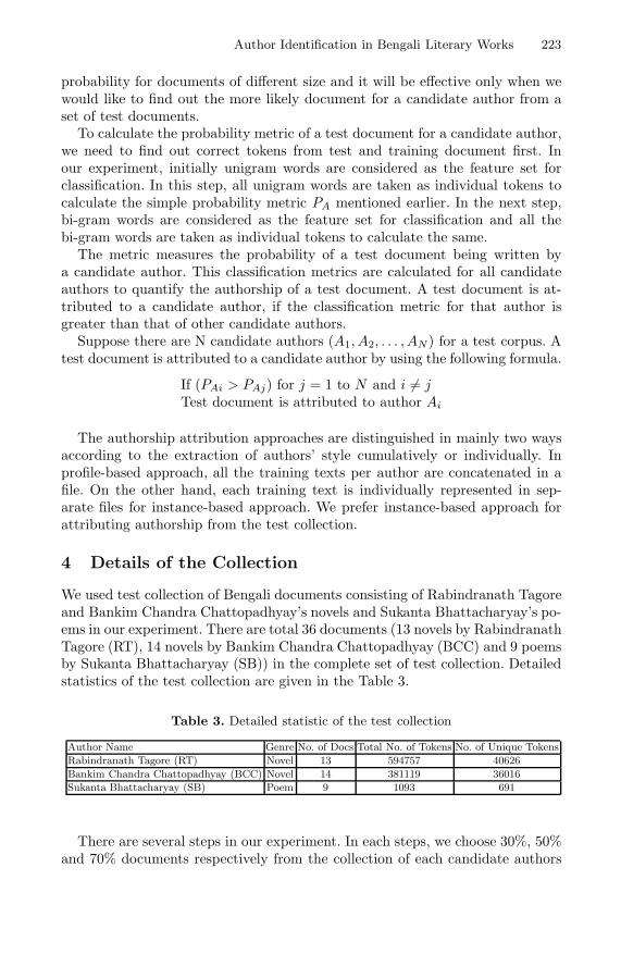
Author Identification in Bengali Literary Works 223
probability for documents of different size and it will be effective only when wewould like to find out the more likely document for a candidate author from aset of test documents.
To calculate the probability metric of a test document for a candidate author,we need to find out correct tokens from test and training document first. Inour experiment, initially unigram words are considered as the feature set forclassification. In this step, all unigram words are taken as individual tokens tocalculate the simple probability metric PA mentioned earlier. In the next step,bi-gram words are considered as the feature set for classification and all thebi-gram words are taken as individual tokens to calculate the same.
The metric measures the probability of a test document being written bya candidate author. This classification metrics are calculated for all candidateauthors to quantify the authorship of a test document. A test document is at-tributed to a candidate author, if the classification metric for that author isgreater than that of other candidate authors.
Suppose there are N candidate authors (A1, A2, . . . , AN ) for a test corpus. Atest document is attributed to a candidate author by using the following formula.
If (PAi > PAj) for j = 1 to N and i = jTest document is attributed to author Ai
The authorship attribution approaches are distinguished in mainly two waysaccording to the extraction of authors’ style cumulatively or individually. Inprofile-based approach, all the training texts per author are concatenated in afile. On the other hand, each training text is individually represented in sep-arate files for instance-based approach. We prefer instance-based approach forattributing authorship from the test collection.
4 Details of the Collection
We used test collection of Bengali documents consisting of Rabindranath Tagoreand Bankim Chandra Chattopadhyay’s novels and Sukanta Bhattacharyay’s po-ems in our experiment. There are total 36 documents (13 novels by RabindranathTagore (RT), 14 novels by Bankim Chandra Chattopadhyay (BCC) and 9 poemsby Sukanta Bhattacharyay (SB)) in the complete set of test collection. Detailedstatistics of the test collection are given in the Table 3.
Table 3. Detailed statistic of the test collection
Author Name Genre No. of Docs Total No. of Tokens No. of Unique Tokens
Rabindranath Tagore (RT) Novel 13 594757 40626
Bankim Chandra Chattopadhyay (BCC) Novel 14 381119 36016
Sukanta Bhattacharyay (SB) Poem 9 1093 691
There are several steps in our experiment. In each steps, we choose 30%, 50%and 70% documents respectively from the collection of each candidate authors

224 S. Das and P. Mitra
as training data set. The selection of training data set was done randomly. Theremaining documents are attributed on the basis of this training data set. Divi-sion of the whole corpus into training set and test set are tabulated in Table 4,when 30%, 50% and 70% of data from individual authors are used for training.
Table 4. Division of whole corpus into training set and test set when 30%, 50% and70% data used for training
30% data used for training 50% data used for training 70% data used for trainingAuthorName
No. ofdocs
No. of docs intraining set
No. of docsin test set
No. of docs intraining set
No. of docsin test set
No. of docs intraining set
No. of docsin test set
RT 13 4 9 7 6 9 4
BCC 14 4 10 7 7 10 4
SB 9 3 6 4 5 6 3Total 36 11 25 18 18 25 11
5 Experimental Results
All the experiments have been done on the test corpus, mentioned earlier. Inthe first stage of our experiment, unigram words and vocabulary richness aretaken as feature set. In this case at first 30% of documents from the collectionof each candidate authors are selected randomly to train the classifier. So outof total 36 documents, 11 documents are selected for training set. Remaining25 documents are classified on the basis of the training data set. In the nextstep, 50% and 70% data from each author are used for training and remainingdocuments are classified. Lastly each and every document is classified when allthe remaining documents are used as training set. The percentages of correctlyclassified documents, taken unigram words as the feature set, are tabulated inthe Table 5.
Table 5. Rate of correctly classified documents when unigram words are taken asfeature set
No. of docs in training set No. of docs tobe classified
No. of correctlyclassified docs
Percentage of cor-rect classification
11(30% from each candidate authors) 25 19 76.00%
18 (50% from each candidate authors) 18 14 77.78%
25 (70% from each candidate authors) 11 9 81.82%
35 (All the documents except the test case) 36 33 91.67%
From this observation, it is seen that the percentage of correct classificationis improved with increasing size of training set.
In the next stage, same thing has been done except the selection of feature set.As feature set, bi-gram words and vocabulary richness are selected in this case.Similarly 30%, 50% and 70% data from individual authors is trained to classifyremaining documents on the basis of new feature set. Then every document is
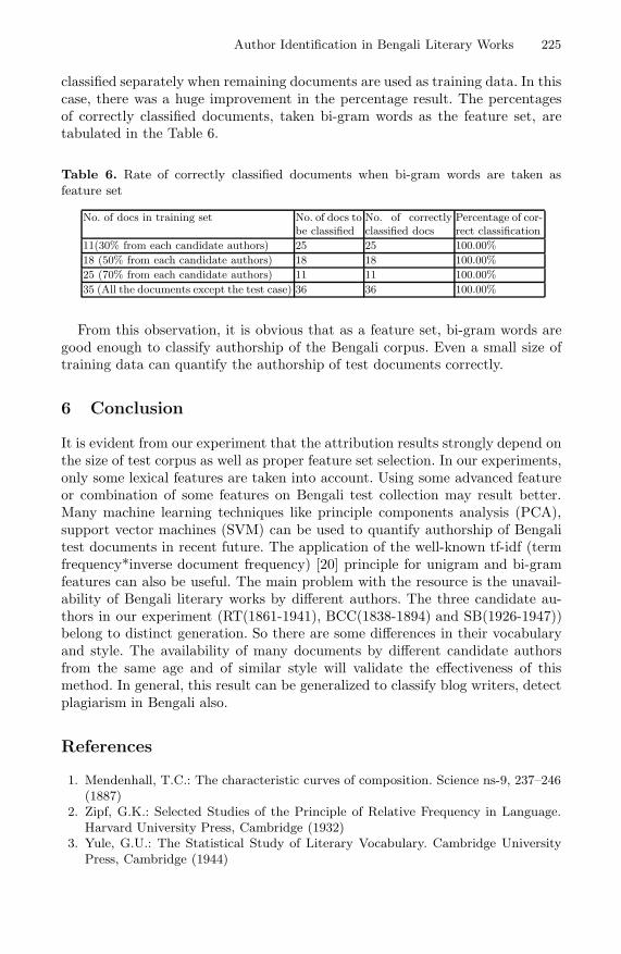
Author Identification in Bengali Literary Works 225
classified separately when remaining documents are used as training data. In thiscase, there was a huge improvement in the percentage result. The percentagesof correctly classified documents, taken bi-gram words as the feature set, aretabulated in the Table 6.
Table 6. Rate of correctly classified documents when bi-gram words are taken asfeature set
No. of docs in training set No. of docs tobe classified
No. of correctlyclassified docs
Percentage of cor-rect classification
11(30% from each candidate authors) 25 25 100.00%
18 (50% from each candidate authors) 18 18 100.00%
25 (70% from each candidate authors) 11 11 100.00%
35 (All the documents except the test case) 36 36 100.00%
From this observation, it is obvious that as a feature set, bi-gram words aregood enough to classify authorship of the Bengali corpus. Even a small size oftraining data can quantify the authorship of test documents correctly.
6 Conclusion
It is evident from our experiment that the attribution results strongly depend onthe size of test corpus as well as proper feature set selection. In our experiments,only some lexical features are taken into account. Using some advanced featureor combination of some features on Bengali test collection may result better.Many machine learning techniques like principle components analysis (PCA),support vector machines (SVM) can be used to quantify authorship of Bengalitest documents in recent future. The application of the well-known tf-idf (termfrequency*inverse document frequency) [20] principle for unigram and bi-gramfeatures can also be useful. The main problem with the resource is the unavail-ability of Bengali literary works by different authors. The three candidate au-thors in our experiment (RT(1861-1941), BCC(1838-1894) and SB(1926-1947))belong to distinct generation. So there are some differences in their vocabularyand style. The availability of many documents by different candidate authorsfrom the same age and of similar style will validate the effectiveness of thismethod. In general, this result can be generalized to classify blog writers, detectplagiarism in Bengali also.
References
1. Mendenhall, T.C.: The characteristic curves of composition. Science ns-9, 237–246(1887)
2. Zipf, G.K.: Selected Studies of the Principle of Relative Frequency in Language.Harvard University Press, Cambridge (1932)
3. Yule, G.U.: The Statistical Study of Literary Vocabulary. Cambridge UniversityPress, Cambridge (1944)
226 S. Das and P. Mitra
4. Mosteller, F., Wallace, D.L.: Inference and Disputed Authorship: The Federalist.Addison-Wesley, Reading (1964)
5. Burrows, J.F.: Word patterns and story shapes: The statistical analysis of narrativestyle. Literary and Linguistic Computing 2, 61–70 (1987)
6. Burrows, J.F.: Not unles you ask nicely: The interpretative nexus between analysisand information. Literary and Linguistic Computing 7, 91–109 (1992)
7. Binongo, J.N.G., Smith, M.W.A.: The application of principal component analysisto stylometry. Literary and Linguistic Computing 14, 445–466 (1999)
8. Holmes, D.I., Robertson, M., Paez, R.: Stephen crane and the new-york tribune:A case study in traditional and non-traditional authorship attribution. Computersand the Humanities 35, 315–331 (2001)
9. Burrows, J.F.: Delta: a measure of stylistic difference and a guide to likely author-ship. Literary and Linguistic Computing 17, 267–287 (2002)
10. Burrows, J.F.: The englishing of juvenal: Computational stylistics and translatedtexts. Style 36, 677–699 (2002)
11. Kjell, B., Woods, W.A., Frieder, O.: Information retrieval using letter tuples withneural network and nearest neighbor classifiers. In: IEEE International Conferenceon Systems, Man and Cybernetics, Vancouver, BC, vol. 2, pp. 1222–1225 (1995)
12. Baayen, H., Van Halteren, H., Tweedie, F.: Outside the cave of shadows: Usingsyntactic annotation to enhance authorship attribution. Literary and LinguisticComputing 11, 121–132 (1996)
13. Juola, P., Baayen, H.: A controlled-corpus experiment in authorship identificationby cross-entropy. Literary and Linguistic Computing 20, 59–67 (2005)
14. Zhao, Y., Zobel, J.: Searching with style: Authorship attribution in classic lit-erature. In: Proceedings of 30th Australasian Conference on Computer Science,vol. 62, pp. 59–68 (2007)
15. Stamatatos, E.: Author identification: Using text sampling to handle the classimbalance problem. Information Processing & Management 44, 790–799 (2008)
16. Koppel, M., Schler, J., Argamon, S., Messeri, E.: Authorship attribution with thou-sands of candidate authors. In: Proceedings of the 29th ACM SIGIR, pp. 659–660.ACM Press, New York (2006)
17. Mansur, M., UzZaman, N., Khan, M.: Analysis of n-gram based text categorizationfor bangla in a newspaper corpus. In: Proceedings of 9th International Conferenceon Computer and Information Technology, Dhaka, Bangladesh (2006)
18. Stamatatos, E.: A survey of modern authorship attribution methods. Journal ofthe American Society for Information Science and Technology 60, 538–556 (2009)
19. Mitchell, T.M.: Machine Learning. McGraw-Hill, New York (1997)20. Manning, C., Raghavan, P., Schutze, H.: Introduction to Information Retrieval.
Cambridge University Press, Cambridge (2008)

Finding Potential Seeds through Rank Aggregation ofWeb Searches
Rajendra Prasath and Pinar Ozturk
Department of Computer and Information Science (IDI)Norwegian University of Science and Technology (NTNU)
Sem Sælands Vei 7-9, NO - 7491, Trondheim, Norwayrajendra,[email protected]
Abstract. This paper presents a potential seed selection algorithm for webcrawlers using a gain - share scoring approach. Initially we consider a setof arbitrarily chosen tourism queries. Each query is given to the selected Ncommercial Search Engines (SEs); top m search results for each SE are obtained,and each of these m results is manually evaluated and assigned a relevance score.For each of m results, a gain - share score is computed using their hyperlinksstructure across N ranked lists. Gain score of each link present in each of mresults and a portion of the gain score is propagated to the share score of each ofm results. This updated share scores of each of m results determine the potentialset of seed URLs for web crawling. Experimental results on tourism related webdata illustrate the effectiveness of the proposed seed selection algorithm.
Keywords: Web Crawlers, Seed Selection, Link Data, Relevant Judgment.
1 Introduction
Online web documents, specifically in textual form, are massively growing and popularsearch engines process (SEs) these documents using the Information Retrieval (IR)components namely: crawler, indexer and searcher as shown in Figure 1. For a given setof Uniform Resource Locators(URL), the crawler fetches the content of the URLs, theindexer facilitates a comprehensive storage of the extracted content from each URL,through indexes, and the searcher estimates similarity between a user query and theindexed documents. Since searching the web upon each query would require processingmillions of pages, a searcher makes the search on a smaller subset of documentscollected through seed URLs and returns the top m results. The results of a particularsearch engine may not include the best possible web pages the user is interested in.Correspondingly, if a user queries for certain information, different search enginesprovide differently ranked top m search results. Two factors mainly determine thequality of search results: similarity judgment and seed URLs. The former is popularlyknown as “web ranking”. The latter should be a good representative of the web in orderto retrieve maximum number of relevant documents. However, it is often not, leadingto inadequate relevant results.
Currently at: Dept of CSE, Indian Institute of Technology, Kharagpur - 721 302, India; email:[email protected]; [email protected]
S.O. Kuznetsov et al. (Eds.): PReMI 2011, LNCS 6744, pp. 227–234, 2011.c© Springer-Verlag Berlin Heidelberg 2011
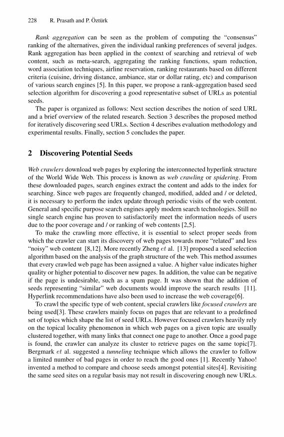
228 R. Prasath and P. Ozturk
Rank aggregation can be seen as the problem of computing the “consensus”ranking of the alternatives, given the individual ranking preferences of several judges.Rank aggregation has been applied in the context of searching and retrieval of webcontent, such as meta-search, aggregating the ranking functions, spam reduction,word association techniques, airline reservation, ranking restaurants based on differentcriteria (cuisine, driving distance, ambiance, star or dollar rating, etc) and comparisonof various search engines [5]. In this paper, we propose a rank-aggregation based seedselection algorithm for discovering a good representative subset of URLs as potentialseeds.
The paper is organized as follows: Next section describes the notion of seed URLand a brief overview of the related research. Section 3 describes the proposed methodfor iteratively discovering seed URLs. Section 4 describes evaluation methodology andexperimental results. Finally, section 5 concludes the paper.
2 Discovering Potential Seeds
Web crawlers download web pages by exploring the interconnected hyperlink structureof the World Wide Web. This process is known as web crawling or spidering. Fromthese downloaded pages, search engines extract the content and adds to the index forsearching. Since web pages are frequently changed, modified, added and / or deleted,it is necessary to perform the index update through periodic visits of the web content.General and specific purpose search engines apply modern search technologies. Still nosingle search engine has proven to satisfactorily meet the information needs of usersdue to the poor coverage and / or ranking of web contents [2,5].
To make the crawling more effective, it is essential to select proper seeds fromwhich the crawler can start its discovery of web pages towards more “related” and less“noisy” web content [8,12]. More recently Zheng et al. [13] proposed a seed selectionalgorithm based on the analysis of the graph structure of the web. This method assumesthat every crawled web page has been assigned a value. A higher value indicates higherquality or higher potential to discover new pages. In addition, the value can be negativeif the page is undesirable, such as a spam page. It was shown that the addition ofseeds representing “similar” web documents would improve the search results [11].Hyperlink recommendations have also been used to increase the web coverage[6].
To crawl the specific type of web content, special crawlers like focused crawlers arebeing used[3]. These crawlers mainly focus on pages that are relevant to a predefinedset of topics which shape the list of seed URLs. However focused crawlers heavily relyon the topical locality phenomenon in which web pages on a given topic are usuallyclustered together, with many links that connect one page to another. Once a good pageis found, the crawler can analyze its cluster to retrieve pages on the same topic[7].Bergmark et al. suggested a tunneling technique which allows the crawler to followa limited number of bad pages in order to reach the good ones [1]. Recently Yahoo!invented a method to compare and choose seeds amongst potential sites[4]. Revisitingthe same seed sites on a regular basis may not result in discovering enough new URLs.
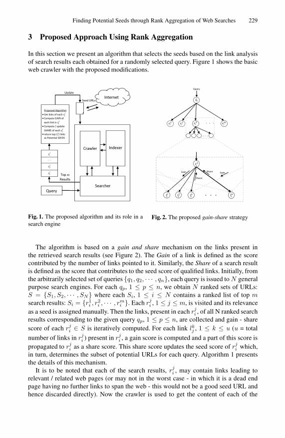
Finding Potential Seeds through Rank Aggregation of Web Searches 229
3 Proposed Approach Using Rank Aggregation
In this section we present an algorithm that selects the seeds based on the link analysisof search results each obtained for a randomly selected query. Figure 1 shows the basicweb crawler with the proposed modifications.
Indexer
Internet
Crawler
Searcher
Query
2
1
. . .
Proposed Algorithm
• Get links of each
• Compute GAIN of
each link in
• Compute / update
SHARE of each
• return top links
as Potential SEEDS
Top m
Results
Seed URLs
Update
Fig. 1. The proposed algorithm and its role in asearch engine
Share
Query
2
1 . . .
GainGain Share
⋅ ⋅ ⋅
. . .
3
3
1
2 3
Fig. 2. The proposed gain-share strategy
The algorithm is based on a gain and share mechanism on the links present inthe retrieved search results (see Figure 2). The Gain of a link is defined as the scorecontributed by the number of links pointed to it. Similarly, the Share of a search resultis defined as the score that contributes to the seed score of qualified links. Initially, fromthe arbitrarily selected set of queries q1, q2, · · · , qn, each query is issued to N generalpurpose search engines. For each qp, 1 ≤ p ≤ n, we obtain N ranked sets of URLs:S = S1, S2, · · · , SN where each Si, 1 ≤ i ≤ N contains a ranked list of top msearch results: Si = r1
i , r2i , · · · , rm
i . Each rji , 1 ≤ j ≤ m, is visited and its relevance
as a seed is assigned manually. Then the links, present in each rji , of all N ranked search
results corresponding to the given query qp, 1 ≤ p ≤ n, are collected and gain - sharescore of each rj
i ∈ S is iteratively computed. For each link lkj , 1 ≤ k ≤ u (u = total
number of links in rji ) present in rj
i , a gain score is computed and a part of this score ispropagated to rj
i as a share score. This share score updates the seed score of rji which,
in turn, determines the subset of potential URLs for each query. Algorithm 1 presentsthe details of this mechanism.
It is to be noted that each of the search results, rji , may contain links leading to
relevant / related web pages (or may not in the worst case - in which it is a dead endpage having no further links to span the web - this would not be a good seed URL andhence discarded directly). Now the crawler is used to get the content of each of the

230 R. Prasath and P. Ozturk
retrieved search results. This content is first segmented into blocks and the noisy blocksare eliminated using link - to - text ratio. Here Link - to - text ratio is defined as the ratiobetween the size of the text tagged with hyperlinks and the text without hyperlinks. Thispossibly eliminates noisy blocks from the web document using the structural propertiesof the underlying mark up language and presents the valid blocks. From these validblocks, outgoing links are collected and used to estimate the gain - share scores.
Algorithm 1. Seed Selection Algorithm using Link Interrelatedness Based Scoring
Input: A query having d terms: Q = t1, t2, · · · , tdTop ranked n URLs of N SEs: Si = rj
i | 1 ≤ i ≤ N & 1 ≤ j ≤ n;threshold - The update limit for the share score at the parent link;
Procedure:1: For each rj
i , seed score(rji ) ← ∅;
2: for each search engine ∈ N do3: For given q, retrieve top m URLs and assign Share(rj
i ) := 0.0;4: for each retrieved URL rj
i ∈ R do5: seed score(rj
i ) ← manual relevance judgment in 0-1 scale &UrlsInPage ← ∅;
6: Obtain valid blocks of rji using link-to-text ratio ;
7: Extract links lkj from valid blocks of rji & URLsInPage ← insert(lkj );
8: max = #(overlapping lkj ∈ URLsInPage);9: for each lkj ∈ URLsInPage do
10: Gain(lkj ) ← 0.0 & Compute/update the gain of lkj using Equation. 1;11: if ( Gain(lkj ) < threshold ) then12: Discard lkj from URLsInPage; max = max− 1;13: else14: Update Share(rj
i ) using Equation 2;15: end if16: end for17: seed score(rj
i ) ← Share(rji )
18: end for19: end for20: return top l URLs, sorted by seed score(rj
i ), as SEEDS
Output: Top l SEED URLs sorted by their seed score in the decreasing order
For each search result, we obtain m URLs (delivered by one of the SEs) eachof which is stored in UrlsInPagej where 1 ≤ j ≤ m. Then we apply the rankaggregation process on each lkj , where 1 ≤ k ≤ n in each search result and obtainthe gain scores.
Gain(lkj ) = Gain(lkj ) +#OL(rj
i )
rank(rji )
× seed score(rji ) (1)

Finding Potential Seeds through Rank Aggregation of Web Searches 231
where rji = P (lkj ) - the parent of link lkj ; #OL(rj
i ) = Total number of outgoing links
from rji ; rank(rj
i ) = v ∀v, 1 ≤ v ≤ n. Initially, gain is assumed to be zero.In the proposed algorithm, we have just used the outgoing links from the search
engine results rji , but in principle, one could use several levels of outgoing links from rj
i .Thus the algorithm could be generalized where gain - share score is computed iterativelyover a chain of links. Each of these links propagate a certain amount of share of theirgain score to its parent (actual search results) to support it as a good seed. We term thefinal share score as the seed score.
Share(rji ) = Share(rj
i ) + (Gain(lkj )/max) (2)
where max - the number of overlapping outgoing links of search results across Nsearch result sets for each corresponding query.
This score will be shared with the corresponding search result in the bottom upfashion and will support the search result for becoming a good candidate in seedselection. This is repeated for all links present in all subsets and then the top m searchresults of N search engines. Once we complete the gain - share computations for all topm search results which are then aggregated and based on their new seed score and topm links were selected as the potentially good seed URLs.
4 Evaluation and Discussions
We have selected 10 tourism queries (in English) from Cross Lingual InformationAccess (CLIA) Project - a major project for CLIA in Indian languages, funded bythe Government of India, and being executed by a consortium of several academicinstitutions and industrial partners 1. Each query is presented in three forms: title -the actual query, desc - the expanded query and narr - the narration of the query. Herewe consider each query either with ( title and / or desc). The structure of each query isshown in Figure 3 and selected list of queries are given in the Figure. 4.
4.1 Dataset and Evaluation Strategy
We have collected URLs of top n = 30 search results for each of the queries given inFigure 4 using four commercial search engines: Google, Yahoo!, Bing and Cuil duringSeptember 2010. Thus for each query, we have collected 120 ( = 4 search engines eachwith top 30) search results which may be disjoint or may partly overlap across thesearch results of different search engines. We repeated this process for all 10 querieslisted in the Figure 4 and collected 1200 web pages. Some of the links were obsolete,modified or removed. All these 1200 web pages were visited manually and relevanceof each was judged in the scale of real numbers between 0 and 1 with 0.1 steps. Theactual overlap among the search results of 4 search engines are listed in Table 1 and therank of these overlapping URLs across 4 search results are different. We measure thegoodness of seeds (in turn, the goodness of the crawl created by the ranked seed set) byPrecision measure. Precision (P) is the fraction of retrieved documents that are relevant.We measure P@d (“Precision top d documents”) with d = 10.
1 http://www.clia.iitb.ac.in/clia-latest

232 R. Prasath and P. Ozturk
<topics> <top lang=”en”>
<num>4</num><title>Trekking in Darjeeling</title><desc>Find documents reporting on the trekking
expedition in Darjeeling</desc><narr>Relevant document should report on thetrekking expeditions in Darjeeling, the breathtakingview of the surrounding landscape, flora and fauna,the names of the popular treks like the Sandakphutrek, the Kalimpong trek etc, the different trekkingroutes,the necessary clothing and equipment fortrekking, the best months for trekking and informationregarding different tour packages provided for thetourists.</narr>
</top></topics>
Fig. 3. Query in XML format
QID Query (title)Q1 Amritsar and the Golden TempleQ2 Rishikesh Water RaftingQ3 Toy train ShimlaQ4 Mumbai Ganesh FestivalQ5 Sunderbans National Park and its tourist
attractionsQ6 Cuisine of Tamil NaduQ7 Goa its beautiful beachesQ8 Sun Temple at KonarkQ9 Meghalaya and its virgin beauty
Q10 Trekking in Darjeeling
Fig. 4. Selected 10 CLIA Queries
Table 1. Overlapping URLs among 300 [10 Queries × Top 30] Results
# Engines Google Yahoo! Bing CuilGoogle 0 90 108 38Yahoo! 90 0 108 29Bing 108 108 0 32Cuil 38 29 32 0
4.2 Relevance Judgement
During the manual relevant judgement, we focus particularly on the search resultsleading to the “intent” of user’s queries. Since the domain being tourism, it is natural toget lots of web content related to tour packages or planning trips (schedulers), or havingforms for booking accommodation or transport. So we have given less importance tosuch contents and more to the focused content of the web documents. During manualevaluation, we have made some observations which mimic the characteristics of thecommercial search engines. Some of the search results for the given query leads tovideo information and may be visually related to the given query. But it is not useful forthe systems handling textual content or users having the intent in exploring the historybehind the query. In a query related to “trekking”, most of the pages contain schedulesand plans about the trekking packages offered at various nearby hilly places. Forumdiscussions / answers describing the user experiences on a specific feature - may beevent or place or hotel - are obtained for queries having proper name.
We eliminated the outdated or invalid results by marking it as -1. A few search resultscontained information about the subtopic of the given query than fetching the overallintent of the query. Such pages were proportionately marked with score deductions.The search results having site replications at different URLs were ranked in the list.For example, page having URL like “http://www.abc.com” and “http://abc.com” wereconsidered as single entity and it is hardly possible to avoid this in the automated webcrawling.

Finding Potential Seeds through Rank Aggregation of Web Searches 233
4.3 Discussions
Here we present the experimental results of the proposed method on selected tourismrelated queries. Out of total 1200 search results [ = 10 Queries x top 30 results x 4search engines], we have identified 320 links that are common across search resultsof different search engines. Hence 26% of same search results repeat on an averagefor top 10 queries. We have noticed similar amount of search results between Googleand Yahoo! search engines. However the number of matching results between Googleand Bing is high and Google and Cuil is low (please refer to Table 1). This forms afair distribution among the search results across different search engines for differentqueries. During the preliminary analysis, we found that if more number of child linkinfluence the gain - share score, then it is essential to modify the threshold so that moreand more hyperlinked pages, even though they are irrelevant, would hardly dominatethe score propagation.
First we selected top 40 urls for each query and crawled them to the depth 2. Nowfor each query, we have manually checked the precision @ top d (=10) documents scorefor selected queries(refer to Figure 6). The proposed method diverges in some cases forexample, Q10 - “Trekking in Darjeeling”, there are lots of pages with Nepal expeditionsand Himalayan expeditions rather than focusing on Sandakphu and Kalimpong Treks.We have done this experiment with only 1200 relevant judged web documents andhence the diversity of the seed selection would be attempted with more data.
0
20
40
60
80
100
120
140
Q1 Q2 Q5 Q6 Q7 Q8 Q2 Q3 Q10
Effect of gain - share in seed selection Gain
Share
score
Queries →
See
d s
co
re
→
Fig. 5. Seed Score variations for the SelectedQueries
0
1
2
3
4
5
6
7
8
Q1 Q2 Q4 Q5 Q7 Q8 Q10
Effectiveness of Seeds
P@10 -Actual
P@10 -proposed
Queries - >
P @
10
- >
Fig. 6. P@10 Scores
Figure 5 shows the preliminary results of our experiments towards seed selectionamong the selected queries. Here we have highlighted special cases in which manualjudgment score is lower, but the gain - share score is considerably higher. This indicatesthat this seed could be a better candidate for selecting as the seed URL. Similarly theseed for the query Q8 which ranked 7 in the ranked list with partial relevance can be abetter choice due to its link structures. These links carry forward to the relevance linksin a few steps. In the sequel, we would like to experiment more in comparison with therecent web crawler seed selection algorithms.

234 R. Prasath and P. Ozturk
5 Conclusion
In this paper, we proposed a seed selection algorithm for web crawlers using link datawith gain - share based approach. The proposed method would capture the potentialseeds from the ranked search results of commercial search engines in an indirectway. This approach could also be generalized to find better seeds by accounting thecrawling to various depths. Analyzing the commercial search results can model thecharacteristics in finding good candidates towards computing the “interestingness” of apage(in turn, relevance to the user query). In our future work, attempts would be madeto dynamically modify, update and / or remove the outdated URLs [9,10].
References
1. Bergman, M.K.: The deep web: Surfacing hidden value. Journal of Electronic Publishing 7(1)(August 2001)
2. Brin, S., Page, L.: The anatomy of a large-scale hypertextual web search engine. In: WWW7:Proceedings of the seventh international conference on World Wide Web 7, pp. 107–117.Elsevier Science Publishers B.V., Amsterdam (1998)
3. Chakrabarti, S., van den Berg, M., Dom, B.: Focused crawling: a new approach to topic-specific web resource discovery. Comput. Netw. 31(11-16), 1623–1640 (1999)
4. Dmitriev, P.: Host-based seed selection algorithm for web crawlers. US Patent(US20100114858A1) (May 2010)
5. Dwork, C., Kumar, R., Naor, M., Sivakumar, D.: Rank aggregation methods for the web.In: WWW 2001: Proceedings of the 10th international conference on World Wide Web, pp.613–622. ACM, New York (2001)
6. Hawking, D., Craswell, N.: Which search engine is best at finding online services? In:Proceedings of WWW10, Hong Kong (2001)
7. Micarelli, A., Gasparetti, F.: Adaptive focused crawling. Springer, Heidelberg (2007)8. Niu, C., Li, W., Ding, J., Srihari, R.K.: A bootstrapping approach to named entity
classification using successive learners. In: ACL 2003: Proceedings of the 41st AnnualMeeting on Association for Computational Linguistics, pp. 335–342. Association forComputational Linguistics, Morristown, USA (2003)
9. Pal, S.K., Talwar, V., Mitra, P.: Web mining in soft computing framework: relevance, stateof the art and future directions. IEEE Transactions on Neural Networks 13(5), 1163–1177(2002), http://dx.doi.org/10.1109/TNN.2002.1031947
10. Rumelhart, D.E., Hinton, G.E., Williams, R.J.: Learning internal representations by errorpropagation. MIT Press, Cambridge (1986)
11. Smucker, M.D., Allan, J.: Using similarity links as shortcuts to relevant web pages. In: SIGIR2007: Proceedings of the 30th annual international ACM SIGIR conference on Research anddevelopment in information retrieval, pp. 863–864. ACM, New York (2007)
12. Yangarber, R.: Counter-training in discovery of semantic patterns. In: ACL 2003:Proceedings of the 41st Annual Meeting on Association for Computational Linguistics, pp.343–350. Association for Computational Linguistics, Morristown, USA (2003)
13. Zheng, S., Dmitriev, P., Giles, C.L.: Graph based crawler seed selection. In: WWW 2009:Proceedings of the 18th international conference on World wide web, pp. 1089–1090. ACM,New York (2009)

Combining Evidence for Automatic Extraction
of Terms
Boris Dobrov and Natalia Loukachevitch
Research Computing Center of Lomonosov Moscow State University,Leninskie Gory, 4/1, Moscow, Russia
dobroff,[email protected]
Abstract. The paper describes the method of extraction of two-worddomain terms combining their features. The features are computed fromthree sources: the occurrence statistics in a domain-specific text collec-tion, the statistics of global search engines, and a domain-specific the-saurus. The evaluation of the approach is based on the terminology ofmanually created thesauri. We show that the use of multiple featuresconsiderably improves the automatic extraction of domain-specific terms.We compare the quality of the proposed method in two different domains.
Keywords: term acquisition, thesaurus, Internet search, machinelearning.
1 Introduction
Technical terms represent domain-specific concepts in domain documents. Itmeans that terms are key elements to understanding of the conceptual structureof the domain. Therefore automatic extraction of domain-specific terms fromtexts is a subject of constant interest in automatic processing of documents.The special difficulty is the automatic extraction of multiword terms [1].
When working with large subject areas and text collections, even the bestmethods for extracting terminological collocations show significant drop in termpercentage from 90% in the first hundred of the list, down to 60% in the thirdthousand. Thus, an important problem is development of new methods to im-prove the quality of phrase ordering to increase the percentage of terms at thetop.
For many years researchers tried to find the best statistical feature for termextraction. Now machine learning methods allow for the combination of manyfeatures. Thus, in [2] the combination of different statistical characteristics ofphrases, based on the Czech text collection, is used to extract different types ofcollocations (such as phrasal verbs or idioms). The authors used over 80 featuresand obtained 20% improvement compared with the best individual feature. Butthe authors of this paper indicate that efficiency of different features is veryvariable and depends on a collection, types of expressions and so on.
In this paper we describe an experiment to extract two-word terms based on acombination of three types of features: features based on a domain-specific text
S.O. Kuznetsov et al. (Eds.): PReMI 2011, LNCS 6744, pp. 235–241, 2011.c© Springer-Verlag Berlin Heidelberg 2011
236 B. Dobrov and N. Loukachevitch
collection, features obtained from an Internet search engine and features obtainedfrom a domain-specific thesaurus. Working with a thesaurus we simulate thesituation when a thesaurus partially exists. We want to study its potential torecognise new terms. The important point of our research is to study the stabilityof the term extraction model among different domains.
2 Description of Experiment: Data and Evaluation
We conduct our study in two domains. The first domain is the very broad domainof natural sciences and technologies. The second domain is domain of bankingand bank regulation. For both domains we have Russian domain-specific thesaurideveloped manually, which we use as a basis for evaluation of term extractionmethods. The current volume of Ontology on Natural Sciences is more than 140thousand terms [3]. Banking thesaurus includes about 15 thousand terms.
Besides we have Russian domain-specific text collections used for develop-ment of these thesauri. From the text collections we have extracted single wordsand multiword expressions. Two-word expressions belong to two types of noungroups: Adjective+Noun and Noun+Noun in Genitive. The extracted expres-sions were ordered in descending order of their frequencies. Our experts workedwith these term candidate lists paying more attention to expressions with highfrequencies. However it was noted that the important terms could have mediumor low frequencies because of the unbalance of the text collections. So the aim ofour new term extraction method is to reorder the extracted expressions to pro-vide the presence of more approved terms in the beginning of the candidate list.We experimented with five thousands of the most frequent two-word expressionsfrom these candidate lists.
To evaluate the reordering quality of methods we use the measure of aver-age precision adopted from information retrieval [4]. Average precision AvP inthe task of extracting terminological expressions is calculated as follows. Sup-pose that in an ordered list of expressions there are k terms, and pos (i) -position of the i-th term from the beginning of the list. Then the precision onthe level of the i-th terminological expression PrecT ermi in an ordered list isPrecTerm(pos(i)), that is the value of precision PrecT ermi is calculated atthe time of inclusion to the list of i-th term and is equal to the percentage ofterms in the list from 1 to pos (i) positions. Average precision for the givenordered list is equal to the average value of PrecT ermi:
AvP =1k
∑
i
PrecTermi
Measure of average precision allows us to estimate the quality of term ex-traction with a single value because the more domain terms are located in thebeginning of the list the more is the value of average precision.

Combining Evidence for Automatic Extraction of Terms 237
3 Features for Term Candidate Reordering
For extracted phrases we compute features of three types. First, we use featurescalculated on the basis of the domain-specific text collection. In this experimentsuch features are the frequency of the phrase, mutual information (MI),MI3 (the same as MI but accounts the cube of the phrase frequency [5]) andInsideness. Insideness is calculated as the inverse ratio of the phrase frequencyto maximal frequency of a three-word phrase comprising the given phrase.
We use not so many features from the domain-specific text collection becauseour main interest is to study other types of features based on Internet searchand known terms desribed in a domain-specific thesaurus. We will consider thesetypes of features in the following subsections.
3.1 Features Based on Internet Search
Internet-based features were obtained with xml-interface of Russian Search En-gine Yandex on the basis of specially formulated queries. For our experimentswe utilised so-called search snippets - short fragments of texts explaining searchresults. Example of one of Yandex snippets for phrase internal debt is asfollows:
Internal debt is the part of a country’s debts that is owed to creditors whoare citizens of that country. It is a form of fiat creation of money, in which thegovernment obtains cash not by printing it, but by borrowing it.
Use of Internet search for term extraction is important for the following rea-sons. First, the domain-specific text collection is always not sufficient because alot of fairly significant terms of the domain may have relatively low frequenciesin it. Involvement of the Internet helps us get additional information on suchterms. Secondly, the use of information from the Internet allows us to find outif a given phrase is rigidly connected with the domain.
To calculate phrase features, 100 snippets from search results were utilised.Snippets from the same query were merged into one document and processed bythe morphological processor. As a result, for each set of snippets lemmas (wordsin a dictionary form) were extracted and their frequencies of occurrence werecalculated. For every query, we obtain a vector of lemmas with correspondingfrequencies. Snippets are generated for the whole phrases and its constituentwords. We denote Sab - a vector of lemma frequencies derived from phrase snip-pets, Sa, Sb - vectors of lemmas from constituent word snippets. From suchvectors, the following types of features were calculated.
The first group of features are scalar products of snippet vectors: < Sab, Sa >(Scalar1), < Sab, Sb > (Scalar2). Also we calculated scalar products of Booleanvariants of snippet vectors (elements of vectors are from 0, 1) : < Sbab, Sba >(Boolean1), < Sbab, Sbb > (Boolean2). These features compare overall dis-tinctions in lexical contexts of a phrase and its components.
The frequency of a phrase in its own snippets (FreqBySnip). We sup-posed that if the value of this feature is significantly greater than 100 (sometimes

238 B. Dobrov and N. Loukachevitch
this feature reached 250-300 occurrences in 100 snippets), it means that thereare many contexts, in which this phrase is explained in detail, is the theme ofthe fragment, and, most likely, this phrase denotes an important concept or aspecific entity.
Features of semantically specific context (SnipFreqi). Many domain-specific mulltiword terms have sense specificity, which can not be deduced fromits components. This specificity of the term can be shown in additional rela-tions to other terms not directly related to intial term components. To find suchspecificity we extract a single lemma that is very frequent in phrase snippetsand absent (or rarely mentioned) in component snippets.
Let lemma L occur fab times in phrase snippets, fa, fb times occur in snippetsof components. Then we calculate SnipFreq0 feature as follows:
SnipFreq0 = maxL
fab−a−b logN − dLcol
dLcol
wherefab−a−b = max(fab − fa − fb, 0),dlcol is a lemma frequency in documents of a contrastive collection, N - is
the number of documents in the contrastive collection. Factor log(
N−dLcol
dLcol
)is
so called idf-factor known from information retrieval research [4], it helps todiminish influence of frequent general words. The contrastive collection is thecollection of documents of Belorussian Internet distributed in the framework ofRussian seminar on information retrieval (www.romip.ru/ en/index.html).
SnipFreq1 and SnipFreq2 features are calculated in similar way exceptingwords in a window of 1 (2) words near every occurrence of ab phrase. Thesevariants of SnipFreq feature are intended to remove partial fragments of longerterms from consideration.
Number of definitional words in snippets (NearDefWords). This featurecalculates overall frequency of so called definitional words in phrase snippets.These words (as type, class, define etc.) are often used in dictionary definitions.Therefore their presence in snippets can mean that a snippet contains a definitionof this phrase or the phrase is used in definition of other term. NearDefWordsfeature is equal to the number of these definitional words that appeared imme-diately adjacent (left or right) with the original phrase in snippets.
Number of marker words in snippets (Markers). This feature denotesnumber of five-ten the most important words of the domain in snippets of theexpression. For the natural science domain these words were as follows: mathe-matics, mathematical, physics, physical, chemisry, chemical, geology, geological,biology, biological.
Number of Internet page titles (SnipTitle). We calculated number of In-ternet page titles coinciding with a given phrase, because we supposed that use ofthe expression in the title of an Internet page stresses significance of the phrase.

Combining Evidence for Automatic Extraction of Terms 239
3.2 Features Based on Terms of Domain-Specific Thesaurus
In many domains there are well-known terms and even information-retrievalthesauri. The third type of our features is based on the assumption that theknown terms can help to predict unknown terms. For the experiments in twodomains, we used the relevant thesauri. If a phrase was a thesaurus term, then itwas excluded from the terminological basis for feature generation. We consideredthe following features obtained from a domain-specific thesaurus.
Synonym to Thesaurus Term (SynTerm). Documents of the domain cancontain a lot of variants of the same term [6]. Therefore we can suppose that aphrase similar to a thesaurus term is also a term. Let a and b be components ofphrase ab. We consider phrase cd as a synonym of ab phrase if every componentword of phrase cd is either equal to a component word of ab either is a synonymof a component word of ab. The order of components in a phrase is unimportant.
Synonym to Non-Term (SynNotTerm). We also fix a feature of similarityto a phrase not included to the thesaurus.
Completeness of Description (Completeness). It is possible that compo-nent words a and/or b of phrase ab have been already described in the domainthesaurus as domain terms. Completeness feature is a sum of thesaurus relationsof component terms in the thesaurus.
4 Results of Experiments
We experimented in two domains: the banking domain and the domain of naturalsciences. In all experiments, 5 thousand most frequent two-word expressions ex-tracted from the corresponding text collections were used. For these expressionsall above-mentioned features were calculated. To obtain the best combinationof features generating the best reordering, we used machine learning methodsimplemented in programming package RapidMiner (www.rapidminer.com). Thequality of reordering was evaluated with AvP measure. The training set wasthree-quarters of the phrase list, the testing set was a quarter. As basic minimallevels of AvP we used the alphabet order and the decreasing frequency order.
We tested various machine learning methods from RapidMiner package. Everytime logistic regression achieved maximal level of AvP. Therefore we took thismethod as a basic method of machine learning for our experiments in termextraction. The table 1 shows values of AvP for single features and results oflogistic regression method.
SynTerm and SynNotTerm features are Boolean and can not be evaluatedwith AvP. We concluded that SynTerm feature is highly informative: if Syn-Term (ab) =1 then phrase ab is a domain term with probability of more than80%.
We can see that in both cases the same set of features and use of machinelearning methods lead to much higher values of average precision. However thereare significant distinctions in ratios between AvP of features. For example, in
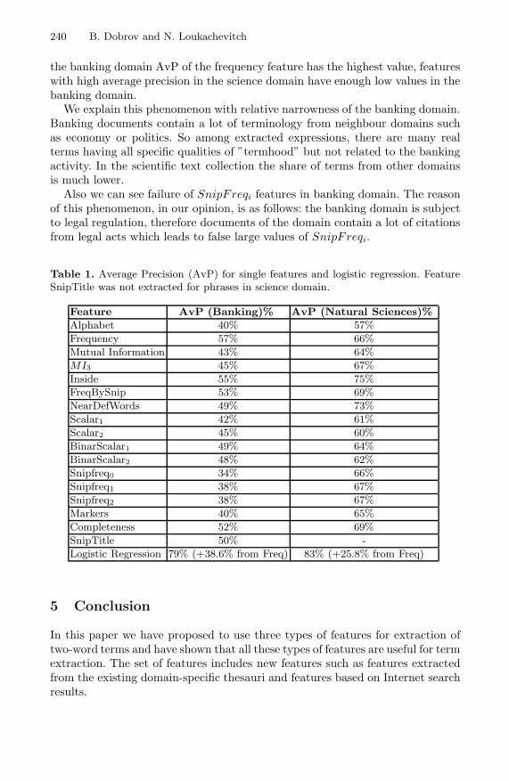
240 B. Dobrov and N. Loukachevitch
the banking domain AvP of the frequency feature has the highest value, featureswith high average precision in the science domain have enough low values in thebanking domain.
We explain this phenomenon with relative narrowness of the banking domain.Banking documents contain a lot of terminology from neighbour domains suchas economy or politics. So among extracted expressions, there are many realterms having all specific qualities of ”termhood” but not related to the bankingactivity. In the scientific text collection the share of terms from other domainsis much lower.
Also we can see failure of SnipFreqi features in banking domain. The reasonof this phenomenon, in our opinion, is as follows: the banking domain is subjectto legal regulation, therefore documents of the domain contain a lot of citationsfrom legal acts which leads to false large values of SnipFreqi.
Table 1. Average Precision (AvP) for single features and logistic regression. FeatureSnipTitle was not extracted for phrases in science domain.
Feature AvP (Banking)% AvP (Natural Sciences)%
Alphabet 40% 57%
Frequency 57% 66%
Mutual Information 43% 64%
MI3 45% 67%
Inside 55% 75%FreqBySnip 53% 69%
NearDefWords 49% 73%
Scalar1 42% 61%
Scalar2 45% 60%
BinarScalar1 49% 64%
BinarScalar2 48% 62%
Snipfreq0 34% 66%
Snipfreq1 38% 67%
Snipfreq2 38% 67%
Markers 40% 65%
Completeness 52% 69%
SnipTitle 50% -
Logistic Regression 79% (+38.6% from Freq) 83% (+25.8% from Freq)
5 Conclusion
In this paper we have proposed to use three types of features for extraction oftwo-word terms and have shown that all these types of features are useful for termextraction. The set of features includes new features such as features extractedfrom the existing domain-specific thesauri and features based on Internet searchresults.

Combining Evidence for Automatic Extraction of Terms 241
We have shown that the combination of several types of features considerablyenhances the quality of the term extraction procedure. The developed systemof term extraction reorders terms in a list of candidates much better than thebasic-line order with decreasing frequency.
We studied the set of features for term extraction in two different domains.We found that developing term extraction models in a specific domain, it isimportant to take into account such properties of the domain as broad scope ornarrow scope (science vs. banking) and relatedness to the socio-political domain,which is regulated with legal acts. We suppose that it is possible to find themain types of domains for term extraction, to select the best feature sets andcorresponding machine learning models for every type of domains.
References
1. Zhang, Z., Iria, J.: Brewster, Ch., Ciravegna, F.: A Comparative Evaluation of TermRecognition Algorithms. In: Sixth International Language Resources and Evalua-tion, LREC 2008 (2008)
2. Pecina, P., Schlesinger, P.: Combining association measures for collocation extrac-tion. In: Annual Meeting of the Association for Computational Linguistics, ACL2006, ACM Press, New York (2006)
3. Dobrov, B., Loukachevitch, N.: Development of Linguistic Ontology on NaturalSciences and Technology. In: Linguistic resources and Evaluation conference, LREC2006 (2006)
4. Manning, C., Raghavan, P., Shutze, H.: Introduction to Information Retrieval. Cam-bridge University Press, Cambridge (2008)
5. Daille, B., Gaussier, E., Lang, J.M.: An evaluation of statistics scores for wordassociation. In: Tbilisi Symposium on Logic, Language and Computation, pp. 177–188. CSLI Publications (1998)
6. Nenadic, G., Ananiadou, S., McNaught, J.: Enhancing automatic term recognitionthrough recognition of variation. In: 20th International Conference on Computa-tional Linguistics (COLING 2004), pp. 604–610 (2004)

A New Centrality Measure for Influence
Maximization in Social Networks
Suman Kundu, C.A. Murthy, and S.K. Pal
Center for Soft Computing ResearchIndian Statistical InstituteKolkata, India - 700108
sumankundu [email protected], [email protected], [email protected]
Abstract. The paper addresses the problem of finding top k influen-tial nodes in large scale directed social networks. We propose a central-ity measure for independent cascade model, which is based on diffusionprobability (or propagation probability) and degree centrality. We use (i)centrality based heuristics with the proposed centrality measure to get kinfluential individuals. We have also found the same using (ii) high degreeheuristics and (iii) degree discount heuristics. A Monte-Carlo simulationhas been conducted with top k-nodes found through different methods.The result of simulation indicates, k nodes obtained through (i) signif-icantly outperform those obtain by (ii) and (iii). We further verify thedifferences statistically using T-Test and found the minimum significancelevel (p-value) when k > 5 is 0.022 compare with (ii) and 0.015 whencomparing with (iii) for twitter data.
1 Introduction
Large scale online social networks became popular in recent years. Twitter, Face-book, Orkut, LinkedIn is few examples. These social networks have millions ofusers. People around the globe are connected with the purpose of common in-terests. These applications are becoming a huge marketing platform of productsand services, specially spreading the information to a large number of people ina short amount of time. However, the most important question arises “How toselect the influential individual quickly, to target for marketing?”
Domingos et al. were the first to study the problem as an algorithmic problemand proposed probabilistic methods in [3, 10]. In [5] Kempe et al. formulatedthe problem as a discrete optimization problem and showed that the problem isNP hard. They also proposed a greedy hill climbing approach, which provides(1−1/e−ε) approximation of the optimal solution. Finally, they showed throughexperiments that their approach provides significant improvement over the clas-sical degree, and centrality based heuristic. However, for large scale graphs, thegreedy approach may be time consuming. Chen et al. recently proposed few im-provements of the model in [1]. They provided NewGreedy and further modifiedit to MixedGreedy. Even after the improvement, this approach would take days
S.O. Kuznetsov et al. (Eds.): PReMI 2011, LNCS 6744, pp. 242–247, 2011.c© Springer-Verlag Berlin Heidelberg 2011
A New Centrality Measure for Influence Maximization in Social Networks 243
to run on large scale social networks. So, Chen et al. in [1] provided the de-gree discount heuristic model which runs much faster than the greedy model. In[4], authors provided another approach to solve the problem in less time. Theycalled it set covering greedy algorithm. This algorithm, however, needs moretime compared to the centrality based heuristic models.
In this paper, we propose a centrality measure, diffusion degree, and then weuse it to rank influential individuals of large sample of directed social networks.We simulate the information spread with top k nodes from different algorithmsand compare it with the simulation results of the proposed algorithm. We foundproposed algorithm provides statistically significant improvements.
The paper is organized as follows, in Section 2 we provide the information dif-fusion model. Section 3 describes some related works. In the Section 4, centralitymeasure diffusion degree is described. Section 5 shows experimental results.
2 Information Diffusion Model
Independent Cascade Model: Independent cascade model of information diffusionis proposed by Lopez-Pinatado [6]. It is the most common model for informationdiffusion. In this model, nodes can have two states, either active or inactive.Nodes are allowed to switch from inactive to active but not in the other. Thediffusion model starts with an initial set of active nodes. In time t, an activenode u will get chance to activate its inactive neighbor v. v will become activewith a probability λ called diffusion probability or propagation probability. uwill not get any further chance to activate v. The diffusion probability is a user-defined parameter of the model. The process of diffusion stops when no furtheractivation is possible. This method is called independent because the activationof a node does not depend on the history of active nodes.
3 Related Works
High Degree Heuristic Model: The most classic approach to solve the influencemaximization problem is High Degree Heuristics. Here the influence is calculatedbased on the degree of a node, i.e. if k nodes are required to select as seed thenthe top k high degree node will be selected.
Degree Discount Heuristic Model: General idea of the degree discount algorithmof Chen et al. is that if one node is considered as seed then the links connectingwith the node will not be counted as a degree of the other nodes, i.e. whenconsidering the next node, the links connecting with the nodes already in theseed set will be discounted.
4 Proposed Diffusion Degree and Heuristic Model
Several attempts are made to improve efficiency of the greedy algorithm. How-ever, for a large scale network its efficiency is far from the speed of centrality

244 S. Kundu, C.A. Murthy, and S.K. Pal
based heuristics. Degree is commonly used for finding the seeds of the influencemaximization problem. In [5], Kempe et al. showed through experimental re-sults that high degree heuristics produces a large influence spread compared toother centrality based heuristics. In addition, some of the centrality measureslike betweenness require huge computation load to calculate. In this section, wepropose a centrality measure, diffusion degree based on the diffusion probability.The diffusion degree can be calculated quickly even for large scale networks. Aheuristic model is then described for influence maximization problem.
Many of the available centrality measures considered only structural propertyof a node. However, when considering the diffusion process, diffusion probabilityplays a vital role in influence flow over the network. Additionally, the central-ity based heuristic models did not consider the effect of neighborhood. Take anexample of high degree heuristics, suppose a node (v1) with the highest degreein the network is connected with some low degree nodes. Consider another node(v2) with a less degree; and its neighbors are high degree nodes. Now, the ob-vious choice in the high degree model is v1. In this case, the diffusion processpropagate less level compared to v2 because the neighborhood of v2 can sendthe information to more nodes in the network than neighbors of v1. Our con-tributed centrality measure considers the above mention properties of diffusionmodel and social networks.
The general degree centrality measure is proposed by Nieminen in [9]. Thedegree centrality of node v can be defined as
CD(v) =n∑
i=1
σ(ui, v) (1)
where function σ(ui, v) defined as,
σ(ui, v) = 1 if and only if ui and v are connected= 0 otherwise.
In a diffusion process, a node v with propagation probability λv, can activateits neighbor u with probability λv. So, considerable contribution of node v inthe diffusion process is
C′DD(v) = λv ∗ CD(v). (2)
When the diffusion process propagates to the next level, active neighbors of vwill try to activate their inactive neighbors.Thus the cumulative contribution inthe diffusion process by neighbors of v will be maximized when all of its neighborswill be activated in the previous step. In this scenario, the total contribution ofneighbors of v is
C ′′DD(v) =
∑
i∈neighbors(v)
C′DD(i). (3)
The diffusion degree of a node is defined as the cumulative contribution scoreof the node itself and its neighbors. So, from the equations 2 and 3 we can definethe diffusion degree CDD of node v as

A New Centrality Measure for Influence Maximization in Social Networks 245
CDD(v) = C ′DD(v) + C ′′
DD(v) (4)
= λv ∗ CD(v) +∑
i∈neighbors(v)
C′DD(i) (5)
= λv ∗ CD(v) +∑
i∈neighbors(v)
λi ∗ CD(i). (6)
The diffusion degree measure depends upon the diffusion probability. How-ever, this measure is independent of the nodes already selected. Thus calculat-ing the diffusion degree for every node of the network could be determined inO(N + E) time where N is the number of nodes and E is the number of edgesin the network. In defining the diffusion degree, we consider the effect of imme-diate neighbors to a node because for a small diffusion probability, the effect ofneighbor’s neighbor of a node may be ignored[1].
Our heuristics model works similar to other centrality based heuristics forfinding top k influence maximization problem. The only difference is that we usethe diffusion degree instead of classical centrality measures. The algorithm is asfollows
1. Find diffusion degree (CDD) for all nodes of the network2. Select top k nodes for k-top influence maximization problem.
5 Experiment and Results
In our experiment, we use directed social networks e.g. twitter. In case of di-rected networks like twitter, one person (or node) can influence its followers. Itis unlike that one can influence a person he/she following. So, the out degreeof nodes is ignored in our experiments. We use Monte-Carlo simulations of theindependent cascade model for a sufficiently large number of times to get anaccurate approximation of final influence spread. Reader may refer to [7] foradditional information about Monte-Carlo methods.
We compare our results with other centrality based heuristics. We avoid com-paring results with the greedy approach because for a million node social net-works and Monte-Carlo simulation, even the high end server takes days to com-pute results. Finally, we compare results statistically using T-Test. For moredetails about the T-Test and p-value readers may refer to [8].
5.1 Data Set
Our primary data set for experiment is twitter data used in [2]. It was obtainedby a snowball sampling of the twitter site in late 2009. The data set contains over400K nodes and more than 800K of relations. Unlike twitter, which is directlyrelated to the problem domain, we use DBLP citation network [11] to verify ourclaim. The idea behind experimenting with a different data is to verify whetherthe improvements are only for a particular data set, or it has a similar impact onother real life data sets as well. The DBLP citation network contains over 447Knodes and over 2.3 million relations. Here also, we get better results compare toother centrality based model.
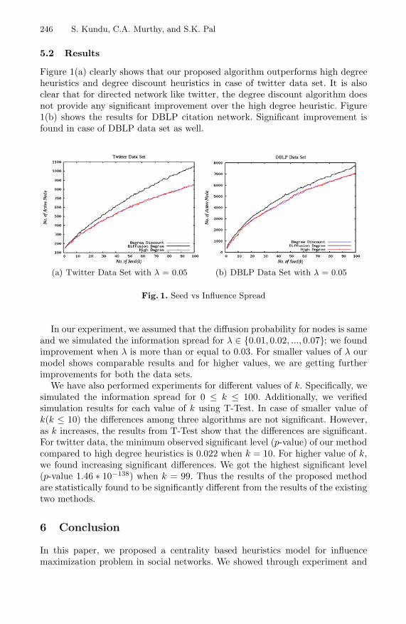
246 S. Kundu, C.A. Murthy, and S.K. Pal
5.2 Results
Figure 1(a) clearly shows that our proposed algorithm outperforms high degreeheuristics and degree discount heuristics in case of twitter data set. It is alsoclear that for directed network like twitter, the degree discount algorithm doesnot provide any significant improvement over the high degree heuristic. Figure1(b) shows the results for DBLP citation network. Significant improvement isfound in case of DBLP data set as well.
(a) Twitter Data Set with λ = 0.05 (b) DBLP Data Set with λ = 0.05
Fig. 1. Seed vs Influence Spread
In our experiment, we assumed that the diffusion probability for nodes is sameand we simulated the information spread for λ ∈ 0.01, 0.02, ..., 0.07; we foundimprovement when λ is more than or equal to 0.03. For smaller values of λ ourmodel shows comparable results and for higher values, we are getting furtherimprovements for both the data sets.
We have also performed experiments for different values of k. Specifically, wesimulated the information spread for 0 ≤ k ≤ 100. Additionally, we verifiedsimulation results for each value of k using T-Test. In case of smaller value ofk(k ≤ 10) the differences among three algorithms are not significant. However,as k increases, the results from T-Test show that the differences are significant.For twitter data, the minimum observed significant level (p-value) of our methodcompared to high degree heuristics is 0.022 when k = 10. For higher value of k,we found increasing significant differences. We got the highest significant level(p-value 1.46 ∗ 10−138) when k = 99. Thus the results of the proposed methodare statistically found to be significantly different from the results of the existingtwo methods.
6 Conclusion
In this paper, we proposed a centrality based heuristics model for influencemaximization problem in social networks. We showed through experiment and
A New Centrality Measure for Influence Maximization in Social Networks 247
statistical tests that it has a significant improvement over other existing central-ity based heuristics for directed networks. We believe our centrality measure,and the heuristic algorithm will provide comparable results for undirected socialnetworks as well.
As a future work, we plan to test the algorithm with other samples of thetwitter and to compare our results with a close optimal value produced by thegreedy approach. In our model, we only considered the Independent CascadeModel. The work may be extended to see the outcomes in other cascade modelsas well.
References
[1] Chen, W., Wang, Y., Yang, S.: Efficient influence maximization in social networks.In: Proceedings of the 15th ACM SIGKDD international conference on Knowledgediscovery and data mining, pp. 199–208. ACM Press, New York (2009)
[2] Choudhury, M.D., Sundaram, H., John, A., Seligmann, D.D., Kelliher, A.: “birdsof a feather”: Does user homophily impact information diffusion in social media?CoRR abs/1006.1702 (2010)
[3] Domingos, P., Richardson, M.: Mining the network value of customers. In: Pro-ceedings of the seventh ACM SIGKDD international conference on Knowledgediscovery and data mining, pp. 57–66. ACM Press, New York (2001)
[4] Estevez, P.a., Vera, P., Saito, K.: Selecting the Most Influential Nodes in SocialNetworks. In: International Joint Conference on Neural Networks, August 2007,pp. 2397–2402 (2007)
[5] Kempe, D., Kleinberg, J., Tardos, E.: Maximizing the spread of influence througha social network. In: Proceedings of the ninth ACM SIGKDD international con-ference on Knowledge discovery and data mining - KDD 2003, p. 137. ACM Press,New York (2003)
[6] Lopez-Pintado, D.: Diffusion in complex social networks. Games and EconomicBehavior 62(2), 573–590 (2008)
[7] MacKay, D.: Introduction to monte carlo methods. Learning in graphical models(1), 175–204 (1998)
[8] Montgomery, D., Runger, G.: Applied Statistics And Probability For Engineers.Wiley, India (2007)
[9] Nieminen, J.: On the Centrality in a Graph. Scandinavian Journal of Psychol-ogy 15, 332–336 (1974)
[10] Richardson, M., Domingos, P.: Mining knowledge-sharing sites for viral market-ing. In: Proceedings of the eighth ACM SIGKDD international conference onKnowledge discovery and data mining - KDD 2002, p. 61 (2002)
[11] Tang, J., Yao, L., Zhang, D., Zhang, J.: A combination approach to web userprofiling. ACM Transactions on Knowledge Discovery from Data V(March), 1–38(2010)

Method of Cognitive Semantic Analysis ofRussian Sentence
Alexander Bolkhovityanov and Andrey Chepovskiy
Higher School of Economics,Moscow, Russia
[email protected],[email protected]
Abstract. In this paper, we propose two mathematical models intendedfor analyzing the Russian sentence to detect noun phrases and particip-ial clauses. Considered algorithms designed on the basis of the proposedmodels can improve procedure of syntactic parsing. Algorithm for par-ticipial clause identification is based on the concept of syntactic relationbetween verb and dependent syntactic units in the Russian language.
1 Introduction
The main task of semantic analysis is creating representation of a text, allowingto correlate the information contained in the text with the knowledge system.The goal of cognitive semantic analysis [1] is formation of such intermediaterepresentation. The creation of mathematical models which help to solve engi-neering problems of text processing requires to solve the problem of cognitivemodeling of a text.
This problem well studied for languages with a simple syntactic structure, forexample English. But it is a complicated task for languages which have morecomplex structure, for example Russian. There are a lot of syntactic relations inthe Russian sentence.
The information about the syntactic structure of the analyzed text requiresformation of the intermediate representation. The result of parsing is representedas a syntactic dependency tree [2], which can be obtained on the basis of syntacticrelations among the constituent elements of the text. Thus, we are faced withthe task of establishing syntactic relations among syntactic units of sentence.
In this paper we propose mathematical models and algorithms, which help usto solve the problem of identifying syntactic relationships among the elements ofthe text completely but in some acceptable approximation for the real systemsof the text processing.
We describe mathematical models for noun phrase and participial clause iden-tification. In Section 2 we propose mathematical models and algorithms for nounphrase and participial clause identification. We note that participial clause iden-tification is based on the concept of syntactic relations between verb and depen-dent syntactic units, noun phrases for example.
S.O. Kuznetsov et al. (Eds.): PReMI 2011, LNCS 6744, pp. 248–253, 2011.c© Springer-Verlag Berlin Heidelberg 2011
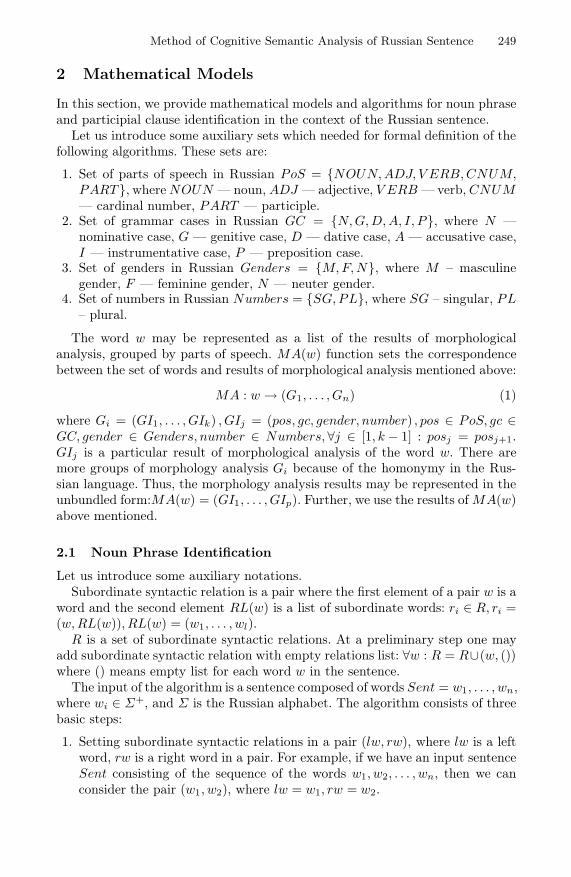
Method of Cognitive Semantic Analysis of Russian Sentence 249
2 Mathematical Models
In this section, we provide mathematical models and algorithms for noun phraseand participial clause identification in the context of the Russian sentence.
Let us introduce some auxiliary sets which needed for formal definition of thefollowing algorithms. These sets are:
1. Set of parts of speech in Russian PoS = NOUN, ADJ, V ERB, CNUM,PART , where NOUN — noun, ADJ — adjective, V ERB — verb, CNUM— cardinal number, PART — participle.
2. Set of grammar cases in Russian GC = N, G, D, A, I, P, where N —nominative case, G — genitive case, D — dative case, A — accusative case,I — instrumentative case, P — preposition case.
3. Set of genders in Russian Genders = M, F, N, where M – masculinegender, F — feminine gender, N — neuter gender.
4. Set of numbers in Russian Numbers = SG, PL, where SG – singular, PL– plural.
The word w may be represented as a list of the results of morphologicalanalysis, grouped by parts of speech. MA(w) function sets the correspondencebetween the set of words and results of morphological analysis mentioned above:
MA : w → (G1, . . . , Gn) (1)
where Gi = (GI1, . . . , GIk) , GIj = (pos, gc, gender, number) , pos ∈ PoS, gc ∈GC, gender ∈ Genders, number ∈ Numbers, ∀j ∈ [1, k − 1] : posj = posj+1.GIj is a particular result of morphological analysis of the word w. There aremore groups of morphology analysis Gi because of the homonymy in the Rus-sian language. Thus, the morphology analysis results may be represented in theunbundled form:MA(w) = (GI1, . . . , GIp). Further, we use the results of MA(w)above mentioned.
2.1 Noun Phrase Identification
Let us introduce some auxiliary notations.Subordinate syntactic relation is a pair where the first element of a pair w is a
word and the second element RL(w) is a list of subordinate words: ri ∈ R, ri =(w, RL(w)), RL(w) = (w1, . . . , wl).
R is a set of subordinate syntactic relations. At a preliminary step one mayadd subordinate syntactic relation with empty relations list: ∀w : R = R∪(w, ())where () means empty list for each word w in the sentence.
The input of the algorithm is a sentence composed of words Sent = w1, . . . , wn,where wi ∈ Σ+, and Σ is the Russian alphabet. The algorithm consists of threebasic steps:
1. Setting subordinate syntactic relations in a pair (lw, rw), where lw is a leftword, rw is a right word in a pair. For example, if we have an input sentenceSent consisting of the sequence of the words w1, w2, . . . , wn, then we canconsider the pair (w1, w2), where lw = w1, rw = w2.

250 A. Bolkhovityanov and A. Chepovskiy
2. Setting syntactic relations inside homogeneous parts of the sentence;3. Identifying of the noun phrases.
Relations are set in the pair (lw, rw). Next, we propose conditions under whichwe add the corresponding relation to the relations set R.
Here are the basic steps of the algorithm.
Setting subordinate syntactic relations
1. If ∃GIi ∈ MA(lw) : posi = NOUN and ∃GIj ∈ MA(rw) : posj = NOUNand gcj = G then add relation for word lw: RL(lw) = RL(lw) ∪ (rw);
2. If ∃GIi ∈ MA(lw) : posi = ADJ and ∃GIj ∈ MA(rw) : posj = NOUN andgci = gcj, geni = genj and either numi = numj or numi = SG then addrelation for word rw: RL(rw) = RL(rw) ∪ (lw);
3. If ∃GIi ∈ MA(lw) : posi = CNUM and ∃GIj ∈ MA(rw) : posj = NOUNand gcj = G and either gci = N or gci = G then add relation for word lw:RL(lw) = RL(lw) ∪ (rw).
Setting syntactic relations inside homogeneous parts of the sentence. Let usintroduce set of copulas C by which homogeneous parts of the sentence are sep-arated. We form the list of homogeneous nouns S = s1, . . . , sm in accordancewith following conditions:
1. Nouns are separated with copula ci ∈ C;2. ∀si ∈ S, ∃sj ∈ S : gci = gcj .
The algorithm is the sequential changing of subordinate syntactic relationsfor nouns from homogeneous parts of the sentence.
If two last nouns sn−1, sn ∈ S are separated with "i" and ∃sl ∈ RL(sn) :∃GIi ∈ MA(sl) : posi = NOUN then if ∀sk ∈ RL(sn−1),¬∃GIi ∈ MA(sk) :posi = NOUN then rn−1 = (sn−1, RL(sn−1) ∪ sl). If ∃GIi ∈ MA(sk) : posi =NOUN then one should finish this part of the second step and perform nextcheck.
If ∀si ∈ S, ∃GIj ∈ MA(si) : gcj = G and if ∃rp ∈ R : s1 ∈ RL(wp) and∃GIj ∈ MA(wp) : posj = NOUN then ∀rq = (wq , RL(wq) if s1 ∈ RL(wq) thenRL(wq) = RL(wq) ∪ (s2, . . . , sm)
Noun phrase identification. We composite an undirected graph GR = (V, E), E =Eq ∪ Eu on the basis of relations from set R. The vertices in this graph are thesentence words, the edges are the subordinate syntactic relation. There are twotypes of edges: u-edges and q-edges. If eql
= (vi, vj) then ∃rp ∈ R : vj ∈ RL(vi)and if eul
= (vi, vj) then ∃rp ∈ R : vj ∈ RL(vi), posvj = ADJ . See Figure 1 forexample.
Noun phrase can be identified by using graph GR. The path p = (v1, . . . , vk)in the graph GR corresponds to the noun phrase if met one of the followingconditions:
1. if k = 2 then e = (v1, v2), e ∈ Eq ;2. if k > 2 then ∃ei ∈ Eu and ∃ej ∈ Eq.
Identified noun phrases form the set NPh = p1, . . . , pf

Method of Cognitive Semantic Analysis of Russian Sentence 251
Fig. 1. Example of the relations graph
2.2 Participial Clause Identification
The algorithm for participial clauses identification works with the set of nounphrases NPh identified with the algorithm which was described in previous sec-tion. Grammatical information for noun phrase is determined by the main wordof the noun phrase. The algorithm is based on the assumption that participlehas the same model of relations with dependent syntactic units as verb fromwhich it is formed. Let us introduce some definitions.
Definition 1. Restriction is a tuple r=(preposition, gc, type) where prepositiondefines preposition with which the verb is used in a sentence, gc defines gram-mar case of the dependence noun phrase, type defines the type of the dependencenoun phrase, which may be free, connected or conditioned.
Definition 2. Relation between verb and dependent syntactic units is a mapthat assigns to each verb in the initial form a list of restrictions:
V R : v → (r1, . . . , rn) (2)
The verb restrictions dictionary has been obtained from the dictionary [5] withsome auxiliary modifications.
There are restrictions for some types of participles, for example the passiveparticiples that supplement the list of restrictions obtained from the participlederived from the verb.
Thus, we can introduce the concept of the relation between participle anddependent syntactic units in the Russian sentence.
Definition 3. Relation between participle and dependent syntactic units is amap that assigns to each participle a list of restrictions:
PR : p → (r1, . . . , rk) (3)
The restrictions for the participle p are obtained from the verb v restrictions andthe additional participle restrictions r1, . . . , rl:
PR(p) = V R(v) ∪ (r1, . . . , rl) (4)

252 A. Bolkhovityanov and A. Chepovskiy
The participial clause is the participle p and dependent noun phrase nph ∈NPh which conforms one of the restrictions from the list PR(p).
Thus, we may formulate the algorithm for participial clause identification:∃wi : ∃GIj ∈ MA(wi) : posj = PART and ∃rp ∈ PR(wi) and ∃nq ∈ NG :prepp ∈ nq , gcp = gcq. Noun phrase nq and participle wi make the participialclause.
3 Evaluation and Example
For evaluation we use the texts from the news corpora on the political topics.The experiments show that the precision of the noun phrases identification isabout 95%. In [3] is shown that for the Russian scientific texts precision is about88%. Own system for noun phrase identification was developed in AOT project.In their paper [4] the authors describe the templates in the regular language.This formalism has some disadvantages. For example, it is impossible to describethe discontinuous noun phrases with the proposed regular language. We note,that our system is devoid of such shortcomings and it can analyze sentences anylevel of complexity.
The precision of the participial clause identification is about 98% and this isconsistent with the results of our preliminary theoretical analysis.
Let us give an example of noun phrase identification algorithm. We havesentence: Ocenki sostoni i perspektiv rossisko konomiki. Denotewords in sentence by letters: Ocenki — A, sostoni — B, perspektiv — D,rossisko — X, konomiki — C. In Figure 2 you can see syntactic relationsgraph between words in sentence.
Fig. 2. Relations graph for sentence from example
As a result of the algorithm we found the following noun phrases (words is inthe canonical form):
1. konomika rossiski;2. perspektiva konomika rossiski;3. sostonie konomika rossiski;4. ocenka perspektiva;5. ocenka sostonie;6. ocenka sostonie konomika;

Method of Cognitive Semantic Analysis of Russian Sentence 253
7. ocenka perspektiva konomika;8. ocenka sostonie konomika rossiski;9. ocenka perspektiva konomika rossiski.
4 Conclusion
In this paper we examined the mathematical models designed to solve a broadclass of problems on cognitive analysis of text information. The algorithms, for-mulated in the terms of the proposed models can efficiently and with high ac-curacy detect dependent syntactical constructions that help us to realize theefficient algorithm of syntactical analysis of the Russian texts. This is achievedby reducing the large number of possible links in the graph arising after mor-phology analysis due to homonymy in the Russian language. This reduction ispossible when we form chains from word combination, preposition and informa-tion about relations between verb or participle and dependent syntactic unit.
References
1. Croft, W., Cruse, D.A.: Cognitive linguistics (Cambridge Textbooks in Linguistics).Cambridge University Press, Cambridge (2004)
2. Jurafsky, D., Martin, J.H.: Speech and Language Processing: An Introduction toNatural Language Processing, Computational Linguistics, and Speech Recognition,2nd edn. Prentice Hall, New Jersey (2008)
3. Belonogov, G.G., Kuznetsov, B.A.: Yazykovye sredstva avtomatizirovannyh infor-matsionnyh sistem (in russian). Nauka, Moscow (1983)
4. Pankratov, D.V., Gershenzon, L.M., Nozhov, I.M.: Opisanie fragmentacii i sintak-sicheskogo analiza v sisteme Dialing. Tehnicheskaya documentacia (2000) (in rus-sian), http://www.aot.ru/
5. Zolotova, G.A.: Sintaksicheskiy slovar: Repertuar elementarnykh edinits russkogosintaksisa (in russian). Nauka, Moscow (1988)

Data Representation in Machine Learning-Based
Sentiment Analysis of Customer Reviews
Ivan Shamshurin
National Research University – Higher School of Economics, School of AppliedMathematics and Informatics,
20 Myasnitskaya Ulitsa, Moscow, 101000, [email protected]
Abstract. In this paper, we consider the problem of extracting opinionsfrom natural language texts, which is one of the tasks of sentiment anal-ysis. We provide an overview of existing approaches to sentiment anal-ysis including supervised (Naive Bayes, maximum entropy, and SVM)and unsupervised machine learning methods. We apply three supervisedlearning methods–Naive Bayes, KNN, and a method based on the Jac-card index – to the dataset of Internet user reviews about cars and reportthe results. When learning a user opinion on a specific feature of a carsuch as speed or comfort, it turns out that training on full unprocessed re-views decreases the classification accuracy. We experiment with differentapproaches to preprocessing reviews in order to obtain representationsthat are relevant for the feature one wants to learn and show the effectof each representation on the accuracy of classification.
Keywords: Supervised Learning, Unsupervised Learning, SentimentAnalysis, K-nearest Neighbor, Naive Bayes method, Jaccard index.
1 Introduction
People need to collect a lot of information to make the right decision. For in-stance, when we choose an object O (car, pass to a health resort) we often askour friends about advantages and disadvantages of O. In this case we wouldvalue opinions of those people, who used O in the past.
It should be noted that subjective estimations from our friends or O-objectcustomers are extremely important because potentially these estimations containmore detailed, comprehensive information about positive and negative featuresof the goods. It arises from the fact that information from official producers oftendirects our attention to the advantages of the object O.
Generally, sentiment classification in Internet data is an essential moderntrend in the text mining [10]. As a result, a program for getting opinion-basedestimates of the car was developed.
There are two fundamental principles: supervised learning and unsupervisedlearning. More detailed information will be given in the next sections of thepaper.
S.O. Kuznetsov et al. (Eds.): PReMI 2011, LNCS 6744, pp. 254–260, 2011.c© Springer-Verlag Berlin Heidelberg 2011
Data Representation in Machine Learning-Based Sentiment Analysis 255
1.1 The Subject of Research and Problems of Sentiment Analysis
In [1] there is an overall survey of the sentiment analysis problems. Themes oftonality defining (a review or comment contains positive, negative or neutralevaluation of a car, film, etc.), objects features detection, summing up opinions,finding out dependent words are analyzed. First of all we are interested in topicsrelated to the tonality defining.
In sentiment analysis a term “object” is used to represent what we attemptto evaluate. In the case of car evaluation the object is a car or its componentsand properties: saloon, economy of fuel, etc.
Let us consider the problems in sentiment analysis in the following fragmentof review:
”(1) The dynamics is 140 h.p.; it is very good, people respect my car on theroad. (2) The ergonomics is 5+. (3) The outside appearance left rivals trailingfar behind. (4) The quality of sound insulation is insufficient. (5) In conclusionI have to say that this car is very nice”.
First of all we have to decide what we want to understand from this review. Inthis text there are sentences with positive valuation (1, 2 and 3) and sentenceswith negative valuation (4). Also for every opinion there is a correspondinghypotactic object. For instance, in the sentence (5) the author says about thecar as a whole, the sentences (1)–(4) are about the dynamics, ergonomics, outsideappearance and the sound insulation correspondingly.
The problem of the implicit object description was investigated in [3]. In acar review we can find sentences like this one: “The fuel economy is great!”. Inthis case we see the explicit cars feature as fuel economy valuation. At the sametime there are sentences with implicit feature valuation: “All information canbe seen”. In this case it is more difficult to define that this positive valuation isabout the speedometer.
In distinction from [3] in the current paper we took into account implicitvaluations in certain experiments. After the analysis of examples of valuationswe have an idea about problems, which appear in sentiment analysis. In thecurrent study the following model will be considered: the object is a car; thetonality will be defined for every car feature: “outside appearance”, “comfort”,“safety”, “reliability”, “running characteristics”.
2 Approaches to Sentiment Analysis
In the section 11 of [4] three supervised learning methods were compared onthe Internet Movie Database (IMDb): Naive Bayes, Maximal Entropy and SVMmethods. The classifiers chose a class (positive or negative) of a review and theaccuracy was 81.5%, 81.0% and 82.9% correspondingly.
Contrary to [1], we do not define the tonality of the whole text about a car,but classify it positive or negative or neutral for every aspect of the car. In thissense we are much closer to [3].

256 I. Shamshurin
In this research authors propose the unsupervised learning for tonality definingfor every feature of the object. Contrary to [3] the speciality of the consideringtask is the fact that we know sentence valuations (i.e. tonality) in advance. Thiscircumstance makes our task more difficult and will decrease the accuracy ofthe classification, because Internet users can write reviews contradictory to theestimates.
Thus our task is not to define the whole tonality of the car review, but to definethe author′s opinion about car features. It is important to note that reviews arenot well structured, the style of narration is free. Some features may be notmentioned in the text. If the review is positive in general, it means that theauthor does not associate the missing feature with negative emotions and wecan tag this feature as positive. That is why the task of defining the tonality ofthe whole text is a subproblem of our task.
3 Empirical Protocol
3.1 Data Collection and Preprocessing
The Supervised Learning needs the database of the opinions with known carsfeature estimates. The comparative analysis of the car-related sites (in Russian)shows that:
- part of them contains opinions without estimates- there are few sites with opinions with estimatesSo, we decided to extract opinion database from the site http://auto.ru, be-
cause this site is well-known, has high reputation and popularity. Every opinionis placed on the individual page and consists of the title, text, feature′s estimates,advantages and disadvantages.
For automatic opinion extraction the programming module was implementedon the Python. As a result, 5098 opinions about 33 car brands were collected.
Every review was transformed into the following structure: text, then theuser′s estimates.
The cross-validation technique [17] was used for obtaining the training andtest sets: 5033 reviews were divided N times (N was approximately 100) intothe training set by randomly selecting 90% of all the reviews and the test set(10% of all the reviews). The resulting error was considered to be the average ofthe errors in each partition.
3.2 Positive and Negative Examples
We should map scores to classes because the source scores are in the five-pointscoring system, and we divide opinions into 2 (positive and negative) and 3(positive, negative, neutral) classes.
scores → classes

Data Representation in Machine Learning-Based Sentiment Analysis 257
Mapping 1Let us define the opinion as positive if it has the scores 4 or 5 and negative if ithas the scores 1, 2 or 3.
1, 2, 3 → negative 4, 5 → positive
But as a rule the opinions with score 4 contain pros and cons, so it is preferableto use opinions with score 5 in supervised learning.
Mapping 2The second type of mapping supposes classifying opinions into three classes:
4, 5 → positive 3 → neutral 1, 2 → negative
3.3 Data Representation
We need to transform the original text into 4 different types of text repre-sentation, with increasing level of linguistic processing. It was done with “py-morphy” - the Python library for morphological analysis of texts in Russian.
Text representation 1: Text of the opinion without digits, punctuation marks,words consisting of one or two letters, latin symbols.
Text representation 2: Text without pronouns, numerals, prepositions, dis-junctive and coordinating conjunctions and parenthesises.
Text representation 3: Phrases of the following types: noun-adjective (withharmony of tenses, cases, gender).
Text representation 4: Normalized adjectives and adverbs.In all representations the ”not” particle is concatenated to the following word.
Explanations to the text representation 3. After every phrase we wroteits concatenation, because some of the adjectives are both positive and negative:“a fast car” is a positive characteristic, “fast conked” is a negative one. So, wehave 5 attributes for learning: “fast”, “car”, “conk”, “fastcar”, “fastconk”.
4 Descriptions of the Methods
4.1 Naive Bayes Method
Naive Bayes Method is a classical machine learning method. We can find itsimplementation in [2]. Since the probability of a document is a small quantity,these measures were computed on a logarithmic scale.
4.2 The Method Based on the Jaccard Measure of Set Similarity
As a result of Naive Bayes learning for every word we have got the conditionalprobabilities of its appearance in every class. We propose the following method

258 I. Shamshurin
of Jaccard measure preprocessing: we can set the thresholds α1 and α2, so thatthree sets of words will be found: G, N and B.
G=word | P (category = “good” | word) ≥ α1P (category = “neutral” | word)
&P (category = “good” | word) ≥ α2P (category = “bad” | word)Likewise we find N and B. Then for every opinion we define T as the set of
words of the opinion. The next stage is the Jaccard measure calculation [4] forpairs G and T , N and T , B and T :
M1 =|T ∩ G||T ∪ G| M2 =
|T ∩ N ||T ∪ N | M3 =
|T ∩ B||T ∪ B|
If the M1 = maxM1, M2, M3 then we tag the opinion as the opinion withpositive estimation of the feature (for example, comfort).
4.3 K-Nearest Neighbor
Every document in the analysis can be represented as the frequency vectors ofthe manually created terms with known tonality:
- positivefantastic, safety, powerful, etc (83 words in Russian)- negativeproblem, bad, poor, etc (84 words in Russian)
For each opinion we assign the term frequency vector. We took words from thedocuments with scores 1 (extremely negative) or 5 (positive) with the weight 2.
When the classifier takes an opinion from the test data, we construct the termfrequency vector and find k nearest neighbors from the train set. We used theEuclidean metric as the measure of vector similarity.
5 First Results
We know the true estimates from the data (each review contains user′s estimate).The machine learning methods provide us with the experimental estimates. So wecan compute the precision and recall [8]. It will be the criterium of the method′saccuracy.
On the “positive”-“negative” classification (mapping 1) the most accurateresults were achieved with the text representation 3 and 4: 63.3% for Bayes clas-sifier and 56.6% for KNN and 68.1% for Jaccard method. In 3-class classification(mapping 2) the similar precisions were achieved.
The poor precision can be caused by the following noise factors:
- Not always users′ estimates correspond to the text: there are some opinionswith scores “1”, but the text of the opinion is extremely positive
- Sometimes in spite of car feature disadvantages in the text, the score is “5”- Sentences which are not related to the car features are encountered in opin-
ions. People describe the prehistory of the car purchase, for example.

Data Representation in Machine Learning-Based Sentiment Analysis 259
For these reasons the train set should contain only the sentences with theopinions about the cars features. It will decrease the noise influence and moreaccurate results may be achieved. For more details see section 6.
6 Learning with Advanced Data Representation
A list of terms-indicators was made. These 33 words include five cars featuresand contain other words which are similar to them: “bracket”, “dynamics”, “au-tomatic gearbox”, “body”, “clearance”, etc.
The most accurate result was achieved on nouns, adjectives, participles, verbsand adverbs from the sentences with the words from the list of terms-indicators.
The results of the sentences with terms-indicators learning, 3-class classifica-tion:
Bayes KNN (k=5) JaccardReliability Running Characteristics ReliabilityPrecision = 0.77 Precision = 0.49 Precision = 0.68Recall = 0.77 Recall = 0.36 Recall = 0.44Comfort ComfortPrecision = 0.66 Precision = 0.65Recall = 0.66 Recall = 0.32Running Characteristics Running CharacteristicsPrecision = 0.72 Precision = 0.62Recall = 0.72 Recall = 0.3
7 Conclusion and Future Work
The comparative analysis of the machine learning methods in sentiment analysiswas performed. The database of the Internet users′ opinions was extracted. Threemethods for cars features estimates defining were tested on it. In general, wesee a significant difference in classification accuracy depending on preprocessingreviews.
It stands to mention that the precision values are not very high (65%-70%),because of the noise in data, specific nature of the opinion texts: free style ofnarration, grammar mistakes.
In the future there is going to be more thorough linguistic processing fordecreasing influence of the noise, in particular, tools for spelling correction, wordsrelation defining and removing homonymy are going to be implemented.
References
1. Liu, B.: Web Data Mining: Exploring Hyperlinks, Contents, and Usage Data.Springer, Heidelberg (2006)
2. Segaran, T.: Programming Collective Intelligence: Building Smart Web 2.0 Appli-cations. O’Reilly, Sebastopol (2007)
260 I. Shamshurin
3. Hu, M., Liu, B.: Mining and summarizing customer reviews. In: ACM SIGKDDInternational Conference on Knowledge Discovery & Data Mining, Seattle, Wash-ington, USA (2004)
4. Berry, M.W., Browne, M.: Lecture notes in data mining. World Scientific Publish-ing Co, Singapore (2007)
5. Giudici, P.: Applied Data Mining. Statistical Methods for Business and Industry.Wiley, Chichester (2003)
6. Hatzivassiloglou, V., McKeown, K.R.: Predicting the Semantic Orientation of Ad-jectives. In: Proceedings of the 35th Annual Meeting of the ACL and the 8th Con-ference of the European Chapter of the ACL, pp. 174–181. ACL, New Brunswick
7. Lutz, M.: Programming Python. O’Reilly, Sebastopol (2010)8. van Rijsbergen, C.V.: Information Retrieval, 2nd edn. Butterworth, London;
Boston (1979)9. Bird, S., Klein, E., Loper, E.: Natural Language Processing with Python. O’Reilly,
Sebastopol (2009)10. Stavrianoui, A., Andritsos, P., Nicoloyannis, N.: Overview and Semantic Issues of
Text Mining. SIGMOD Record 36(3), 23–34 (2007)11. Poirier, D., Bothorel, C., Boulle, M.: Two possible approaches for opinion analysis
in film reviews: statistic and linguistic. In: EMOT-2008: LREC 2008 Workshop onSentiment Analysis: Emotion, Metaphor, Ontology (2008)
12. Williams, G.K., Anand, S.S.: Predicting the Polarity Strength of Adjectives Using-WordNet. In: Third International AAAI Conference on Weblogs and Social Media(2009)
13. Turney, P.D.: Mining the Web for Synonyms: PMI-IR versus LSA on TOEFL.In: Flach, P.A., De Raedt, L. (eds.) ECML 2001. LNCS (LNAI), vol. 2167, pp.491–502. Springer, Heidelberg (2001)
14. Budanitsky, A., Hirst, G.: Semantic distance in WordNet: An experimental,application-oriented evaluation of five measures. In: Workshop on WordNet andOther Lexical Resources, Second meeting of the North American Chapter of theAssociation for Computational Linguistics, Pittsburgh (2001)
15. Turney, P.D.: Thumbs up or thumbs down? semantic orientation applied to unsu-pervised classification of reviews. In: Proceedings of the 40th Annual Meeting ofthe Association for Computational Linguistics (ACL 2002), pp. 417–424 (2002)
16. Huang, A.: Similarity Measures for Text Document Clustering. In: Proceedings ofthe Sixth New Zealand Computer Science Research Student Conference NZCSRSC2008, Christchurch, New Zealand, pp. 49–56 (2008)
17. Geisser, S.: Predictive Inference. Chapman and Hall, New York (1993)

Automatic Retrieval of Parallel Collocations
Valeriy I. Novitskiy
The Moscow Institute of Physics and Technology, Moscow, [email protected]
Abstract. An approach to automatic retrieval of parallel (two-language)collocations is described. The method is based on comparison of syntactictrees of two parallel sentences. The key feature of the method is a sequenceof filters for getting more precise results.
Keywords: NLP, parallel collocations, automatic information extrac-tion, text mining.
1 Introduction
Most of natural languages consist of hundreds of thousands of words. The amountof two-word combinations is ≈ 1010, but only a few of them are real collocations.
In this work we study the problem of extracting parallel collocations. A paral-lel collocation is a combination of a collocation and its translation into anotherlanguage. We are interested in non-trivial literal translations. Parallel colloca-tions make a valuable linguistic resource. For example, they can be used as anauxiliary material by linguists or as a statistical data in different NLP tasks.
The key feature of the approach described in this work is a sequence of heuris-tic filters which help to extract the most valuable collocations. Extraction ofevery possible collocation is intractable, no precise algorithm for the solution ofthis problem is known. Hence, we have to use some simplifications coming tosoft computing of collocations.
Suppose we are given a corpus of parallel texts1. These texts are alignedsentence-to-sentence, which means that we know the matchings between parallelunits of texts (usually a text unit is one sentence). We use a syntactic analyzerto parse the texts and return respective syntactic trees.
The work described in this paper had several goals:
1. Designing an algorithm for automatic collocation retrieval (with some spe-cific restrictions described below).
2. Collecting statistical data to improve the work of syntactic analyzer in use.3. Improving two-language dictionary by adding new translations.4. Creating a Translation Memory database of parallel collocations which can
be used as a reference-book by linguists.
1 Texts and its translations into different language.
S.O. Kuznetsov et al. (Eds.): PReMI 2011, LNCS 6744, pp. 261–267, 2011.c© Springer-Verlag Berlin Heidelberg 2011

262 V.I. Novitskiy
1.1 Environment
In our work we used several tools developed in ABBYY:
1. English-Russian dictionary2. Syntactic analyzer3. Word-to-Word matching algorithm used for sentence aligning.
The dictionary is based on semantic invariants (or classes). For every lan-guage there are several possible realizations of those classes (e.g., “competition”,“gala” and “event” may be placed in one “competition” class). At the same timehomonyms are placed in several classes simultaneously. The corporate dictionaryis comprehensive enough and consists of more than 60 000 classes. Distinguish-ing between homonyms (disambiguation) is done during text analysis and is notdiscussed here.
The syntactic analyzer takes a single sentence and outputs the best syntac-tic tree2 based on internal estimations of quality. The nodes of the tree aresemantic classes and arcs are connections between words. It is possible to getwrong results (incorrect words sense selection). In this case we suppose thateither wrong collocations will not be produced at all (due to differences of syn-tactic trees in different languages) or their frequency will be rather small todelete them by the following filtration procedures. The refinement of syntactictree is attained by parallel analysis of sentences in both languages.
This work does not use such well-known criteria as Mutual Information [2], t-score measure or log-likelihood measure [3], because we choose more predictableselection algorithms. There are many purely statistical algorithms of collocationextraction based on words cooccurrence (e.g., see [4], [5]), but they do not useinformation about connections between words which we are interested in.
In contrast to other works where syntactic information from texts is used [6],we do not restrict our search to two-words collocations, but look for colloca-tions of different length. In this case one encounters the problem of “partial”collocations: partial collocations are parts of some larger collocations. Here weintroduce a new approach to discarding partial collocations.
2 Description of the Method
The algorithm for retrieving collocations can be divided into the following steps:
1. Word-to-word sentence aligning.2. Single language collocations generation.3. Matching collocations of different languages to compose parallel collocations.4. Filtration of infrequent and occasional collocations.
Below we consider each step of the approach in detail.
2 Different representation of sentence structure can be found in [1].

Automatic Retrieval of Parallel Collocations 263
2.1 Word-to-Word Sentence Alignment
We use a dictionary based on semantic invariants, which means that all possiblesynonyms of a word-sense are placed in one semantic class. So the aligningprocess has to solve the following two main problems:
– Homonyms matching (due to possible incorrect semantic variant choice).– Several synonyms in one sentence.
The first problem can be solved rather easily. We can take all possible semanticclasses to which a word can belong and compare them with all possible classesof the opposite word (pic. 1). In the case they do not have empty intersectionwe can consider them as translations of each other.
Ключ
⎧⎪⎪⎪⎪⎨⎪⎪⎪⎪⎩
as a spring. . .• a key to a door• as a solution. . . as a button
⎫⎪⎪⎪⎪⎬⎪⎪⎪⎪⎭
Key
Fig. 1. Semantic classes intersection
The solution of the second problem is based on syntactic trees. We take intoaccount dependencies between words in sentence. For example, we can matchtwo words with better confidence if their parents in syntactic tree correspond toeach other.
We compare all words between two sentences and estimate the “quality” ofeach pair (as a number). Impossible pairs are suppressed by setting prohibitionpenalty. Then we search for the best pairs (by their integral quality). Thus theproblem is reduced to the well-known problem of searching for the best matchingin a bipartite graph. This problem has a polynomial-time solution algorithm, e.g.a so-called “Hungarian algorithm” (see [7]).
2.2 One-Language Collocation Production
Let us impose the following constraints on collocations:
– The number of words in a collocation ranges from one to five.– The result is a subtree of the syntactic tree.– There are no pronouns in collocations.– Syntactic word3 can not be a root of collocation subtree.– We allow only one “gap” of limited size in the linear realization of a colloca-
tion in a sentence.3 Like pronoun, preposition, auxiliary verb and so on.

264 V.I. Novitskiy
2.3 Parallel Collocations Production
We use the results of two previous steps, namely the alignment of parallel sen-tences and the set of variants of one-language collocations from the same sen-tences. This information allows us to select one-language collocations and producecandidates for parallel collocations. We impose the following constrains:
– The length difference between a collocation and its translation is less or equalto one word.
– There are some word-to-word correspondences between collocations (thelonger collocation the more correspondences there should be).
– It is possible to have no correspondences for short (1–2 words length) collo-cations. Instead, there should be correspondences between collocation rootsand all of their children in the syntactic tree.
– There are no “outgoing” correspondences (that “go out” from a collocationbut do not “come into” its translation).
During this step all possible collocations are produced. For example, in thecorpus of ≈ 4, 2 bln fragments there are more than 100 bln different collocations.But only 7 bln of them occur twice as frequent and more.
2.4 Filtration
At this step we select only valuable collocations from that variety we got duringthe previous step. The main idea is that stable collocations are rather frequentand (almost) always have the same translation. We will omit collocations thatare infrequent and have different translations. Some other heuristics will be un-covered below.
There are several collocation filters:
1. Removal of rare collocations (preliminary filtration by frequency with lowerthreshold).
2. Removal of collocations with stop words.3. Removal of inner collocations, i.e., those that are parts of another. For ex-
ample, “Organization for Security” is an internal part of “Organization forSecurity and Co-operation in Europe”.
4. Similarly we should remove “outer” collocations that can occasionally appear.For example, “in the United Nations” is the outer collocations to the just“United Nations”.
5. Selection of one translation for each collocations (if it is not too ambiguous).We leave translation if it appears not less than in 70% cases.
6. Final removal of rare collocations.7. Removal of well-known translations (found in the dictionary).
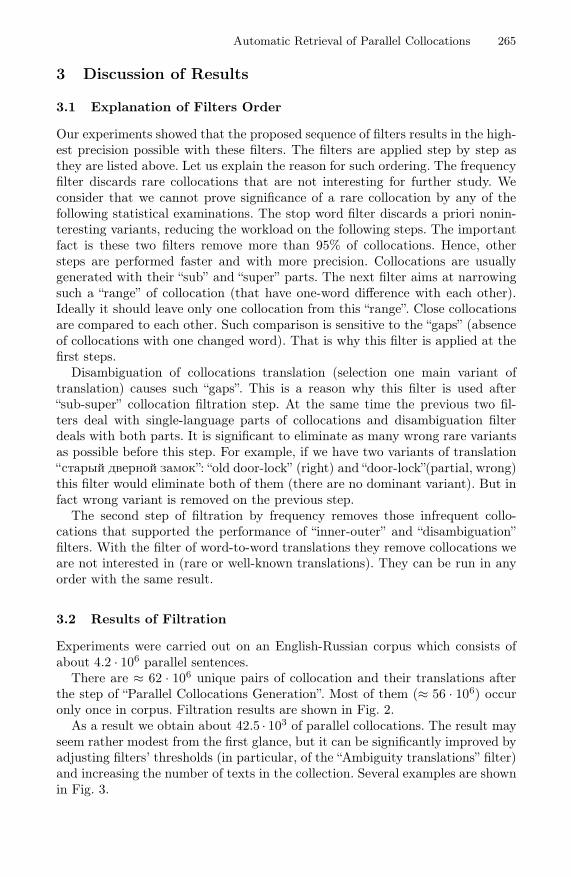
Automatic Retrieval of Parallel Collocations 265
3 Discussion of Results
3.1 Explanation of Filters Order
Our experiments showed that the proposed sequence of filters results in the high-est precision possible with these filters. The filters are applied step by step asthey are listed above. Let us explain the reason for such ordering. The frequencyfilter discards rare collocations that are not interesting for further study. Weconsider that we cannot prove significance of a rare collocation by any of thefollowing statistical examinations. The stop word filter discards a priori nonin-teresting variants, reducing the workload on the following steps. The importantfact is these two filters remove more than 95% of collocations. Hence, othersteps are performed faster and with more precision. Collocations are usuallygenerated with their “sub” and “super” parts. The next filter aims at narrowingsuch a “range” of collocation (that have one-word difference with each other).Ideally it should leave only one collocation from this “range”. Close collocationsare compared to each other. Such comparison is sensitive to the “gaps” (absenceof collocations with one changed word). That is why this filter is applied at thefirst steps.
Disambiguation of collocations translation (selection one main variant oftranslation) causes such “gaps”. This is a reason why this filter is used after“sub-super” collocation filtration step. At the same time the previous two fil-ters deal with single-language parts of collocations and disambiguation filterdeals with both parts. It is significant to eliminate as many wrong rare variantsas possible before this step. For example, if we have two variants of translation“старый дверной замок”: “old door-lock” (right) and “door-lock”(partial, wrong)this filter would eliminate both of them (there are no dominant variant). But infact wrong variant is removed on the previous step.
The second step of filtration by frequency removes those infrequent collo-cations that supported the performance of “inner-outer” and “disambiguation”filters. With the filter of word-to-word translations they remove collocations weare not interested in (rare or well-known translations). They can be run in anyorder with the same result.
3.2 Results of Filtration
Experiments were carried out on an English-Russian corpus which consists ofabout 4.2 · 106 parallel sentences.
There are ≈ 62 · 106 unique pairs of collocation and their translations afterthe step of “Parallel Collocations Generation”. Most of them (≈ 56 · 106) occuronly once in corpus. Filtration results are shown in Fig. 2.
As a result we obtain about 42.5 · 103 of parallel collocations. The result mayseem rather modest from the first glance, but it can be significantly improved byadjusting filters’ thresholds (in particular, of the “Ambiguity translations” filter)and increasing the number of texts in the collection. Several examples are shownin Fig. 3.

266 V.I. Novitskiy
Filter OutputBy frequency (preliminary) 2.5 bln.By stop-word list 1.1 bln.“Inner” and “outer” collocatios ≈ 568 000
Ambiguity translations ≈ 105 000
Translated by dictionary ≈ 66 500
By frequency (finally) 42 636
Fig. 2. Filtration process
English Russian Occurrences
job time срок задания 12galaxy space космическое пространство 13other foreign object иной посторонний объект 5air transport field область воздушного транспорта 30to be beyond the scope of book выходить за рамки книги 29to establish under article учреждать в соответствии со статьёй 75
Fig. 3. Examples of extracted parallel collocations
There are two main measures of results quality: precision and recall. In thiswork the precision is much more important then the recall. The reason is thatit is very difficult to inspect tens of thousand collocation to found ones witherrors. The recall, as the amount of collocations generated, can be made largerwith the growth of the text base. We prefer to omit rare collocations by analyzingmatching errors, however statistical methods like Mutual Information can selectthem as rare and unexpected word combinations. The precision in our researchcomputed by using collocations for analysis of test corpora. We compare resultsof analysis with and without collocations. Any found errors are analyzed andthe general algorithm is updated to avoid them.
An open problem is how an efficient estimate of precision and recall. Man-ual markup of large text bases is almost unfeasible. We estimate precision bycomparing results with opinions of a random subset of experts. Another prob-lem is comparing with statistical algorithms. The comparison is connected withthe difference in produced information (the existence of syntactic links betweenwords in statistical collocations). However, the manual check of random colloca-tions shows good quality in general. An example of such precision estimation isshown in Fig. 4. There are two categories of not good collocations that can berefined by either improving dictionary entities or by customizing the algorithm.An improvement of the algorithm may be attained by eliminating duplicates oftext fragments (that can appear in manuals, government documents and so on).We can achieve precision of more than 80% on this sample by introducing thistechnique.

Automatic Retrieval of Parallel Collocations 267
Quality PercentGood collocations 67Improvable with dictionary 4Improvable with algorithm 16Others 12
Fig. 4. Result of manual checking of a random subset of 100 collocations
4 Conclusion
The main result of our work is a method which proved to be useful and isemployed now in software for collocation search.
There are several possible way to improve the proposed method:
– Introducing a quality measure for collocations (for ranking them and select-ing the best ones).
– Tuning filters thresholds.– Improving corpora used in computations (by correcting spelling errors and
removing occasional bad parallel fragments).
References
1. Bolshakov, I.A.: Computational Linguistics: Models, Resources, Applications. In:Bolshakov, I.A., Gelbukh, A.F. (eds.) IPN - UNAM - Fondo de Cultura Economica(2004)
2. Church, K.W.: Word association norms, mutual information, and lexicography.Computational Linguistics 16(1), 22–29 (1990)
3. Dunning, T.: Accurate methods for the statistics of surprise and coincidence. Com-putational Linguistics 19(1), 61–74 (1993)
4. Smadja, F.A.: Retrieving collocations from text: Xtract. Computational Linguis-tics 19(1), 143–177 (1993)
5. Bouma, G.: Collocation extraction beyond the independence assumption. In: Pro-ceedings of the ACL 2010 Conference Short Papers. ACLShort 2010, pp. 109–114.Association for Computational Linguistics, Stroudsburg, PA, USA (2010)
6. Evert, S.: The Statistics of Word Cooccurences Word Pairs and Collocations. Ph.D.thesis / Universitat Stuttgart. Institut fur Maschinelle Sprachverarbeitung (IMS)(2004)
7. Burkard, R.: Assignment Problems. SIAM, Society for Industrial and Applied Math-ematics, Philadelphia (2009)

Displacement Based Unsupervised Metric for
Evaluating Rank Aggregation
Maunendra Sankar Desarkar, Rahul Joshi, and Sudeshna Sarkar
Department of Computer Science and Engineering,Indian Institute of Technology Kharagpur,
Kharagpur, India - 721302maunendra,rahulrj,[email protected]
Abstract. Rank Aggregation is the problem of aggregating ranks givenby various experts to a set of entities. In context of web, it has appli-cations like building metasearch engines, combining user preferences etc.For many of these applications, it is difficult to get labeled data and theaggregation algorithms need to be evaluated against unsupervised evalu-ation metrics. We consider the Kendall-Tau unsupervised metric which iswidely used for evaluating rank aggregation task. Kendall Tau distancebetween two permutations is defined as the number of pairwise inversionsamong the permutations. The original Kendall Tau distance treats eachinversion equally, irrespective of the differences in rank positions of theinverted items. In this work, we propose a variant of Kendall-Tau distancethat takes into consideration this difference in rank positions. We study,examine and compare various available supervised as well as unsuper-vised metrics with the proposed metric. We experimentally demonstratethat our modification in Kendall Tau Distance makes it potentially bet-ter than other available unsupervised metrics for evaluating aggregatedranking.
Keywords: Information Retrieval, Rank Aggregation, Distance Met-rics, Kendall Tau Distance.
1 Introduction
Rank aggregation problem combines the ranking of entities obtained from mul-tiple ranking functions in order to produce an aggregate ranked list. The inputrankings are referred to as base rankers, or experts. There are various scenarioswhere it is difficult to obtain labeled data and the rankings from different sourcesneed to be aggregated. In such cases, aggregate ranking needs to be evaluatedwith the help of unsupervised metrics. Generally, in such cases, the resultantaggregate ranking is evaluated by average distance with all available rankingsgiven by different experts. Probably the most widely used distance metric usedfor this purpose is Kendall Tau Distance. The Kendall Tau distance is a metricthat counts the number of pairwise disagreements between two ranked lists.
S.O. Kuznetsov et al. (Eds.): PReMI 2011, LNCS 6744, pp. 268–273, 2011.c© Springer-Verlag Berlin Heidelberg 2011
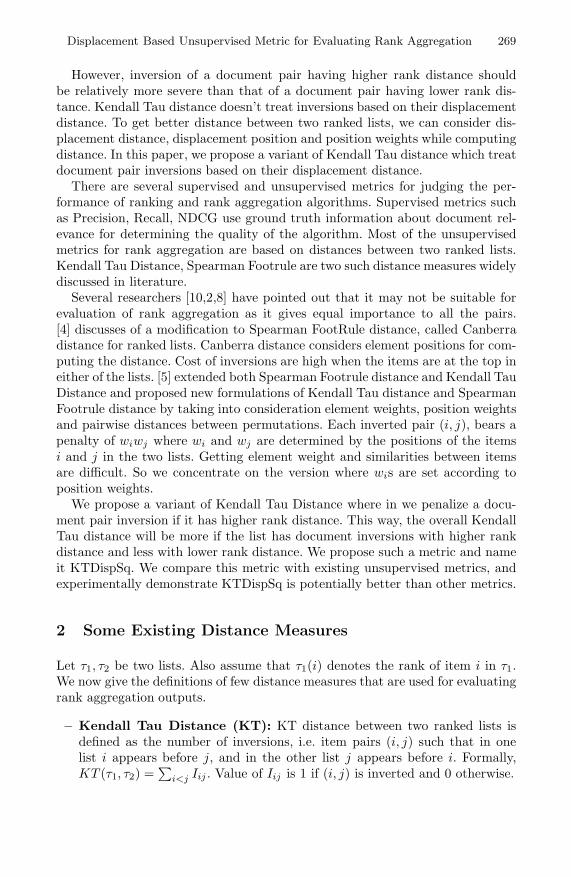
Displacement Based Unsupervised Metric for Evaluating Rank Aggregation 269
However, inversion of a document pair having higher rank distance shouldbe relatively more severe than that of a document pair having lower rank dis-tance. Kendall Tau distance doesn’t treat inversions based on their displacementdistance. To get better distance between two ranked lists, we can consider dis-placement distance, displacement position and position weights while computingdistance. In this paper, we propose a variant of Kendall Tau distance which treatdocument pair inversions based on their displacement distance.
There are several supervised and unsupervised metrics for judging the per-formance of ranking and rank aggregation algorithms. Supervised metrics suchas Precision, Recall, NDCG use ground truth information about document rel-evance for determining the quality of the algorithm. Most of the unsupervisedmetrics for rank aggregation are based on distances between two ranked lists.Kendall Tau Distance, Spearman Footrule are two such distance measures widelydiscussed in literature.
Several researchers [10,2,8] have pointed out that it may not be suitable forevaluation of rank aggregation as it gives equal importance to all the pairs.[4] discusses of a modification to Spearman FootRule distance, called Canberradistance for ranked lists. Canberra distance considers element positions for com-puting the distance. Cost of inversions are high when the items are at the top ineither of the lists. [5] extended both Spearman Footrule distance and Kendall TauDistance and proposed new formulations of Kendall Tau distance and SpearmanFootrule distance by taking into consideration element weights, position weightsand pairwise distances between permutations. Each inverted pair (i, j), bears apenalty of wiwj where wi and wj are determined by the positions of the itemsi and j in the two lists. Getting element weight and similarities between itemsare difficult. So we concentrate on the version where wis are set according toposition weights.
We propose a variant of Kendall Tau Distance where in we penalize a docu-ment pair inversion if it has higher rank distance. This way, the overall KendallTau distance will be more if the list has document inversions with higher rankdistance and less with lower rank distance. We propose such a metric and nameit KTDispSq. We compare this metric with existing unsupervised metrics, andexperimentally demonstrate KTDispSq is potentially better than other metrics.
2 Some Existing Distance Measures
Let τ1, τ2 be two lists. Also assume that τ1(i) denotes the rank of item i in τ1.We now give the definitions of few distance measures that are used for evaluatingrank aggregation outputs.
– Kendall Tau Distance (KT): KT distance between two ranked lists isdefined as the number of inversions, i.e. item pairs (i, j) such that in onelist i appears before j, and in the other list j appears before i. Formally,KT (τ1, τ2) =
∑i<j Iij . Value of Iij is 1 if (i, j) is inverted and 0 otherwise.

270 M.S. Desarkar, R. Joshi, and S. Sarkar
– Spearman Footrule (SF): This metric can be expressed as:∑
i |τ1(i) −τ2(i)|. SF is known to be a 2-approximation of KT.
– Canberra: Canberra distance [4] between two ranked lists τ1 and τ2 is de-fined as:
∑i
|τ1(i)−τ2(i)||τ1(i)|+|τ2(i)| . The denominator ensures that cost of inversions
are high when the items are at the top in either of the lists.
– Position weighted Kendall Tau: We call this measure as PosWtD. Itpenalizes each inversion (i, j) by wiwj where wi and wj are determinedby the positions of the items i and j in the two lists. Mathematically,PosWtD(τ1, τ2) =
∑i<j wiwjIij . Details on how the weights are set can
be found in [5].
3 The Proposed Metric (KTDispSq)
The proposed metric KTDispSq penalizes an inverted pair by an increasing func-tion of the rank distances d1 and d2 for the two lists. More formally, the cost ofeach inversion is defined as:
Ki,j(τ1, τ2) = d21+d2
24n2
Here,
– d1 = absolute rank distance between documents i and j in ranked list τ1
– d2 = absolute rank distance between documents i and j in ranked list τ2
– n = total number of documents in ranked lists τ1, τ2
This way, an inverted docuemnt pair (i, j) with more rank distance in both listsgets penalized more and contributes more in computing distance. The distancebetween two ranked lists is computed as the sum of these penalties over all theinverted pairs.
Example: Consider two ranked lists as
τ1 = [1 4 3 2 5] and τ2 = [1 5 3 4 2].
Here we have four inverted pairs as (2,5) (3,4) (3,5) and (4,5). Inverted pairweights for KTDispSq can be computed as below:
– (2, 5) = (12+32)4∗52 = 0.1
– (3, 4) = (12+12)4∗52 = 0.02
– (3, 5) = (22+22)4∗52 = 0.08
– (4, 5) = (32+22)4∗52 = 0.13
Hence, the total distance KTDispSq between the two lists is: (0.1 + 0.02 +0.08 + 0.13) = .33.
We later experimentally compare the performance of KTDispSq with that ofsome existing unsupervised measures such as KT, Canberra Distance [4], SF,and PosWtD [5].

Displacement Based Unsupervised Metric for Evaluating Rank Aggregation 271
4 Experiments and Results
In order to judge how good the proposed measure is, we propose two sets ofexperiments. Details of the experimental mechanisms, and the results are givenin the following subsections.
We consider Borda[9], QuickSort[9], MC4[3], CombScore[1] as rank aggre-gation methods along with Precision, MAP, Kendall Tau (KT), KTDisp, KT-DispSq, Canberra [4], Spearman Footrule (SF) and PosWtD [5] as metrics. Weworked on LETOR 4.0 MQ2007, MQ2008 and Yahoo LTRC datasets for all ex-periments. These datasets have querywise document scores for various features.We consider each feature as a ranker or an expert. Due to space constraints, wereport results on MQ2007 dataset only.
4.1 Correlation with Other Metrics
In this experiment, we first try several unsupervised rank aggregation algorithmsand evaluate them using the supervised evaluation metrics mentioned above. Theunsupervised metrics compared in this paper are all distance metrics, and lowerscore indicates better quality of the aggregation result. On the other hand, forthe supervised metric MAP, higher score indicates better performance. Hence,a good algorithm should get low score for the unsupervised metrics used in thispaper, but high score for MAP. In other words, if we look at the scores givento the rank aggregation algorithm for different input rankings, then the scoresgiven by the unsupervised metrics should be negatively correlated with the scoresgiven by MAP. We can say that the more negative the correlation, the betterthe unsupervised distance metric.
We use this correlation analysis to compare the performances of the unsuper-vised evaluation measures. Results indicate that our modification makes KendallTau Distance more correlated with MAP. The results are shown in Table 1. KT-DispSq is more negatively correlated for almost all rank aggregation methodswe experimented. For two experiments KTDispSq is second to Canberra, butthe differences are small in those cases. For the remaining experiments, KT-DispSq outperforms others by large margins. This suggests that our variantmakes Kendall Tau more closer to the supervised evaluation metric Mean Aver-age Precision.
Table 1. Correlations with MAP for LETOR MQ2007 dataset. More negative is better.
Borda SumScore MC4 QSort
KT -0.015 -0.112 -0.129 -0.126
KTDispSq -0.058 -0.123 -0.136 -0.134
SF -0.020 -0.109 -0.124 -0.118
Canberra -0.041 -0.124 -0.137 -0.127
PosWtD 0.031 0.240 0.041 0.049

272 M.S. Desarkar, R. Joshi, and S. Sarkar
0.285
0.29
0.295
0.3
0.305
0.31
0.315
0.32
0.325
2 3 4 5 6 7 8 9 10
Pre
cisi
on
KTKTDispSq
SFCanberraPosWtD
(a) Results for Precision
0.23
0.24
0.25
0.26
0.27
0.28
0.29
0.3
0.31
0.32
0.33
2 3 4 5 6 7 8 9 10
ND
CG
KTKTDispSq
SFCanberraPosWtD
(b) Results for NDCG
Fig. 1. Improvement in Precision and NDCG by picking the best expert according tominimum average value of the measures. Higher values are better.
4.2 Pick the Best Expert
In the second set of experiments, we tried to see whether our modificationsenable us to get better output for a rank aggregation task. For this, we tookas experts some widely used features from the test datasets. For each query, wepick the expert which is closest to the remaining experts according to the metricvalue. Mathematically, if R1, R2, · · · , Rn are the input rankings, then we outputas aggregate result Ri such that i = argmini
1n−1
∑nk=1 dist(Ri, Rk). Here dist
represents the distance metric used for selecting the best expert. Features 1, 11,15, 16, 20, 21, 40, 41, 45 were used as experts for these experiments. The featurescorrespond to scores of documents based on tf, tf-idf, BM25, Language Modelscores. Such features are often used for evaluating rank aggregation results [7].Details of the features can be seen from [6].
Figure 1 displays graphically the Precision and NDCG values for the exper-iments. We showed Precision values for rank positions 2, 4, 6, 8 and 10. As the
0.368
0.37
0.372
0.374
0.376
0.378
0.38
0.382
KT KTDispSq SF Canberra PosWtD
MA
P
Unsupervised Evaluation Metrics
MAP
(a) Results for MAP
0.374
0.376
0.378
0.38
0.382
0.384
0.386
0.388
0.39
0.392
0.394
KT KTDispSq SF Canberra PosWtD
Mea
nND
CG
Unsupervised Evaluation Metrics
MeanNDCG
0.374
0.376
0.378
0.38
0.382
0.384
0.386
0.388
0.39
0.392
0.394
KT KTDispSq SF Canberra PosWtD
Mea
nND
CG
Unsupervised Evaluation Metrics
MeanNDCG
0.374
0.376
0.378
0.38
0.382
0.384
0.386
0.388
0.39
0.392
0.394
KT KTDispSq SF Canberra PosWtD
Mea
nND
CG
Unsupervised Evaluation Metrics
MeanNDCG
(b) Results for MeanNDCG
Fig. 2. Improvement in MAP and MeanNDCG by picking the best expert accordingto minimum average value of the measures. Higher values are better.

Displacement Based Unsupervised Metric for Evaluating Rank Aggregation 273
graph suggests, the average Precision and NDCG scores obtained by selecting thelists using our measure are higher than that obtained by using other methods.
We also compared the values of MAP and MeanNDCG for this experiment.Results are shown in Figure 2. For both the measures, higher values indicatebetter performance. Here also we see that the ranked lists selected by usingour measure obtain better scores than others. The results seem to indicate theefficacy of the proposed measure.
5 Conclusions and Future Work
We proposed a displacement based variant of Kendall Tau Distance for evalu-ating aggregated ranking. We can say that displacement based modification inKendall Tau Distance makes it closer to other supervised metrics such as Pre-cision and NDCG. Using KTDispSq in rank aggregation approach gives betterPrecision and NDCG, we can conclude that use of KTDispSq in place of KendallTau Distance may improve Rank Aggregation results. We plan to take into con-sideration position of displacement/inversion of document pair. Displacement atupper ranks should get penalized more than that of lower ranks. We would liketo devise an unsupervised rank aggregation algorithm which directly optimizesthis metric to generate the aggregated ranking.
References
1. Belkin, N.J., Kantor, P., Fox, E.A., Shaw, J.A.: Combining the evidence of multiplequery representations for information retrieval. In: TREC 1995, Elmsford, NY,USA, pp. 431–448. Pergamon Press, Inc., Oxford (1995)
2. Carterette, B.: On rank correlation and the distance between rankings. In: SIGIR2009, pp. 436–443. ACM Press, New York (2009)
3. Dwork, C., Kumar, R., Naor, M., Sivakumar, D.: Rank aggregation methods forthe web. In: WWW 2001, pp. 613–622 (2001)
4. Jurman, G., Riccadonna, S., Visintainer, R., Furlanello, C.: Canberra distance onranked lists. In: Proceedings, Advances in Ranking NIPS 2009 Workshop, pp. 22–27(2009)
5. Kumar, R., Vassilvitskii, S.: Generalized distances between rankings. In: WWW2010, pp. 571–580 (2010)
6. T.-y. Liu, J., Xu, T., Qin, W., Xiong, H.: Li: Letor: Benchmark dataset for researchon learning to rank for information retrieval. In: SIGIR 2007 Workshop on Learningto Rank for Information Retrieval (2007)
7. Liu, Y., Liu, T.-Y., Qin, T., Ma, Z., Li, H.: Supervised rank aggregation. In: WWW,pp. 481–490 (2007)
8. Sanderson, M., Soboroff, I.: Problems with kendall’s tau. In: SIGIR 2007, pp. 839–840 (2007)
9. Schalekamp, F., van Zuylen, A.: Rank aggregation: Together we’re strong. In:ALENEX, pp. 38–51 (2009)
10. Yilmaz, E., Aslam, J.A., Robertson, S.: A new rank correlation coefficient forinformation retrieval. In: SIGIR 2008, pp. 587–594 (2008)

Sentence Ranking for Document Indexing
Saptaditya Maiti1, Deba P. Mandal1, and Pabitra Mitra2
1 Machine Intelligence Unit, Indian Statistical Institute, Kolkata, India2 Dept. of Computer Science and Engineering, Indian Institute of Technology,
Kharagpur, Indiasaptaditya,[email protected],
Abstract. This article discusses a new document indexing scheme forinformation retrieval. For a structured (e.g., scientific) document, Pasi etal. proposed varying weights to different sections according to their im-portance in the document. This concept is extended here to unstructureddocuments. Each sentence in a document is initially assigned weight(significance in the document) with the help of a summarization tech-nique. Accordingly, the term frequency of a term is decided as the sumof weights of the sentences the term belongs. The method is verified on areal life dataset using leading existing information retrieval models, andits performance has been found to be superior to conventional indexingschemes.
Keywords: information retrieval, document indexing, sentence ranking,relative entropy.
1 Introduction
Information retrieval is finding content (usually documents) of an unstructurednature (usually test) that satisfies an information need from within large collec-tion [1]. Information retrieval System (IRS) is based on relevance of a documentto a query. Several methods have been proposed over years. The use of a strongquery and a good retrieval method do not ensure good performance. In fact, theretrieval effectiveness is heavily affected by the model adopted for representingdocuments, since the retrieval mechanism performs a comparison between theuser query and the representation of documents [2][3].
The conventional indexing schemes assume that the information is homoge-neously distributed in documents. Pasi et al. [2][3] claimed that this assumptiondoes not hold for a structured (e.g., scientific) document. The information con-tent of a document varies from one section to another and hence, the terms inthe more important sections should contribute more in retrieval methods. Weargue that this is also true for unstructured documents. Usually, the flow ofinformation in a given document is not uniform, which means that some partsare more important (informative) than others [4]. We know that summarizationtechniques distinguish the more informative parts (i.e., sentences) from the lessones.
S.O. Kuznetsov et al. (Eds.): PReMI 2011, LNCS 6744, pp. 274–279, 2011.c© Springer-Verlag Berlin Heidelberg 2011

Sentence Ranking for Document Indexing 275
In the present investigation, the weight/importance of a sentence in a docu-ment is initially measured with the help of a summarization technique, which istaken here as the relative entropy based method [5]. All of the terms in a sentenceare assumed to have the same weight which is equal to the weight of the sentence.To obtain the term frequency (overall significance) of a term in a document, theweights for each of the occurrences of the term are aggregated. The effectivenessof the proposed indexing scheme is verified for a few leading retrieval models onFIRE dataset [6] and the results are found to be quite encouraging.
The rest of the paper is organized as follows. In section 2, we describe theproposed indexing scheme. The implementation and effectiveness of the schemeis demonstrated in section 3. Section 4 finds the conclusions.
2 Proposed Indexing Scheme
As mentioned earlier, the proposed document indexing scheme is an extensionof the model proposed by Pasi et al. [2][3]. They suggested to provide differentimportance to different sections for indexing structured (e.g., scientific) docu-ments. For example, in a scientific document, the terms in the ‘Title’ carry moreinformation than those in other sections (e.g., ‘abstract’, ‘introduction’, etc.). In[2], different functions for different sections were proposed for providing varyingweights/importance to the terms based on their belongingness in the document.
For the sake of extending the above model, we intend to impose structure toan unstructured document and then to allow varying weights to the terms basedon their positions in the document. We find that extraction based text summa-rization methods analyze the importance/informativeness of different sentencesin a document for selecting a few sentences as the summary of the document.Therefore, summarization techniques may be useful in finding the importance ofthe sentences in a document.
In the current investigation, each sentence in an unstructured document isvisualized as to behave like a section of a structured document. With the helpof a summarization technique, the informativeness of a sentence in a documentis estimated, i.e., a weight is obtained for the sentence signifying its importancein the document.
The proposed indexing scheme consists of two parts. In the first part, weightsof the sentences in a document are obtained using a text summarization method.The second part is concerned with the calculation of the term frequency of eachof the terms in the document.
A) Sentence ranking: A text summarization method is used for ranking thesentences of a document. In this report, we have considered the relative entropybased summarization technique proposed by Kumar et al. [5].
This technique initially estimates the probability of a word w in a sentence Sas
P (w|S) =tf(w, S)
|S| (1)
where tf(w, S) is the frequency of w in S and |S| is the number of words in S.

276 S. Maiti, D.P. Mandal, and P. Mitra
Similarly, the probability of w in a document D is estimated as
P (w|D) =tf(w, D)
|D| (2)
where tf(w, D) is the frequency of w in D and |D| is the number of words in D.A sentence S is provided a weight based on its comparison to the document
D. Comparison is done with relative entropy, i.e., KL-Divergence of S with Das
KLS =∑
w
P (w|S)logP (w|S)P (w|D)
. (3)
As explained in [5], the importance of a sentence, IS , is inversely proportionalto KLS, i.e.,
IS =1
KLS. (4)
We take IS as the weights of the sentences.B) Term frequency: The significance of a sentence in a document is obtained
previously. We assume that the significance is same for all the terms in a sen-tence. Accordingly, we assign the sentence weight to all of its terms. It may berealized that a term belonging to two different sentences may not have the sameinformation content and hence the term may have different scores. Aggregatingthe scores of a term for all of its occurrences in a document, the term frequencyof a term t in D is calculated as
tf(t, D) =∑
Si if tεSi
ISi (5)
The term frequency tf(t, D) as in eqn.(5) reflects the importance of the termin document D based not only on the number of occurrences but also on theinformation content for each of its occurrences. For example, suppose a documenthas the same number of occurrences for two terms t1 and t2, but t1 has appearedin more important sentences than t2. It is easy to realize here that t1 is moresignificant than t2. In such a case, the proposed scheme will find tf value fort1 higher than that of t2 while the conventional indexing schemes will find thesame tf value for both t1 and t2. Hence, the proposed scheme should be a betterindexing scheme than the existing ones which are based on raw counts of terms.
3 Implementation and Results
A new indexing scheme is described in the previous section. The effectivenessof the scheme is verified on the FIRE dataset [6] using Terrier platform [7]. Wehave considered some of the leading retrieval models available in Terrier, namely,Okapi BM25 [8], DFRBM25, InexpB2, InexpC2, IFB2, InL2 and BB2 [9]. A brief

Sentence Ranking for Document Indexing 277
description of these models is provided in Table 1. It is to be noted that all themodels have some parameters which need to be tuned. The parameter valuesmentioned in Table 1 against each model are the ones which are set in theTerrier platform [7] as default and we have used those values in implementingthe models. The results are evaluated here based on Mean Average Precision(MAP).
Table 1. Description of retrieval models considered
Model Description ParameterV aluesConsidered
Okapi BM25 The original BM25 probabilistic model k1=1.2, k2=0,k3=8, b=0.75
DFR BM25 The DFR version of BM25 k1=1.2, k2=0,k3=1000, c=1
In expB2 Inverse expected document frequency model for ran-domness, the ratio of two Bernoulli’s processes for firstnormalisation, and Normalisation 2 for term frequencynormalisation
c=1
In expC2 Inverse expected document frequency model for ran-domness, the ratio of two Bernoulli’s processes for firstnormalisation, and Normalisation 2 for term frequencynormalisation with natural logarithm
c=1
IFB2 Inverse Term Frequency model for randomness, the ra-tio of two Bernoulli’s processes for first normalisation,and Normalisation 2 for term frequency normalisation
c=1
InL2 Inverse document frequency model for randomness,Laplace succession for first normalisation, and Nor-malisation 2 for term frequency normalisation
c=1
BB2 Bose-Einstein model for randomness, the ratio of twoBernoulli’s processes for first normalisation, and Nor-malisation 2 for term frequency normalisation
c=1
For, each of the models, we have experimented with both the conventional(based on raw counts) as well as proposed indexing schemes. In all the cases, themodels with the proposed indexing scheme are found to perform better than thatwith the conventional indexing schemes. The MAP values of the said retrievalmodels with the conventional and the proposed indexing schemes are shown inTable 2. For more clarity, these results are shown graphically in Figure 1.
278 S. Maiti, D.P. Mandal, and P. Mitra
Table 2. MAP of different models with conventional and proposed indexing schemeson FIRE dataset
Indexing Scheme BM25 DFRBM25 InExpB InExpC IFB2 InL2 BB2
Conventional 0.5298 0.5304 0.5347 0.5299 0.5339 0.5420 0.5280
Proposed 0.5732 0.5734 0.5798 0.5744 0.5803 0.5781 0.5747
Fig. 1. MAP of different models with conventional and proposed indexing schemes
4 Conclusions
A new document indexing scheme is proposed in this article. Pasi et al. proposeddifferent importance to terms in different sections of structured documents. Wehave extended this idea to unstructured documents. We assigned different scoresto the sentences of a document using a summarization technique. It is to be men-tioned here that we have taken relative entropy based summarization method forranking the sentences, but one can take any other good summarization method.Instead of taking raw count for term frequency as in conventional indexing meth-ods, we proposed the summation of scores of the sentences the term belongs tobe the term frequency.
We have implemented this scheme in Terrier Platform and tested on FIREdataset for a few leading information retrieval models. In all the cases considered,the performance of this scheme is found to be better than in the conventionalterm frequency. But, to make stronger claims the method is to be tested on moredatasets.

Sentence Ranking for Document Indexing 279
References
1. Manning, C.D., Raghavan, P., Schutze, H.: An Introduction to Information Re-trieval. Cambridge University Press, New York (2008)
2. Bordogna, G., Pasi, G.: Controlling retrieval through a user-adaptive representationof documents. International Journal of Approximate Reasoning 12, 317–339 (1995)
3. Pasi, G.: Fuzzy Sets in Information Retrieval: State of the Art and Research Trends.In: Bustince, H., Herrera, F., Montero, J. (eds.) Fuzzy Sets and Their Extensions:Representation, Aggregation and Models, pp. 517–535. Springer, Heidelberg (2008)
4. Das, D., Martins, A.: A Survey on Automatic Text Summarization. Literature Sur-vey for the Language and Statistics II Course at CMU (2007)
5. Kumar, C., Pingali, P., Varma, V.: A light-weight summarizer based on languagemodel with relative entropy. In: Proc. of the ACM symposium on Applied Comput-ing (SAC 2009). ACM, New York (2009)
6. Forum for Information Retrieval Evaluation (FIRE),http://www.isical.ac.in/~fire/
7. Ounis, I., Lioma, C., Macdonald, C., Plachouras, V.: Research Directions in Terrier:a Search Engine for Advanced Retrieval on the Web. Novatica/UPGRADE, SpecialIssue on Next Generation Web Search 8(1), 49–56 (2007)
8. Robertson, S.E., Walker, S.: Some simple approximations to the 2-poisson modelfor probabilistic weighted retrieval. In: Proc. of 17th Annual Int. Conf. on Researchand Development in Information Retrieval, Dublin, pp. 232–241 (1994)
9. Amati, G.: Probability models for information retrieval based on divergence fromrandomness. Phd thesis, University of Glasgow (2003)
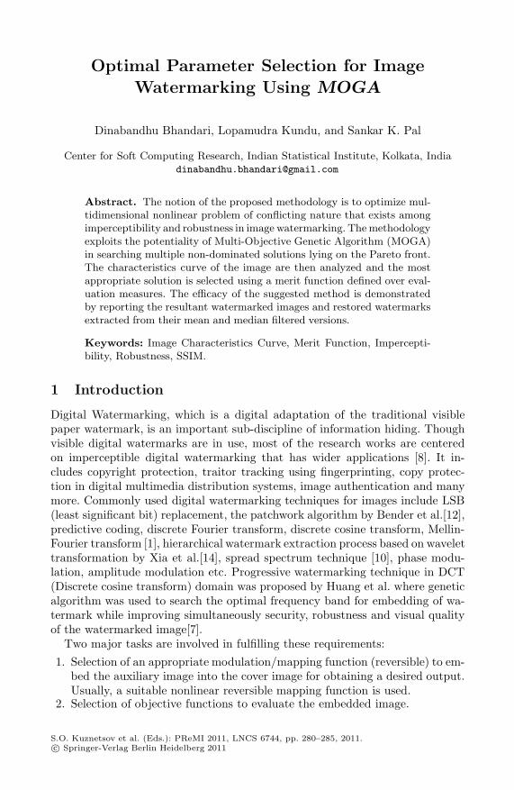
Optimal Parameter Selection for Image
Watermarking Using MOGA
Dinabandhu Bhandari, Lopamudra Kundu, and Sankar K. Pal
Center for Soft Computing Research, Indian Statistical Institute, Kolkata, [email protected]
Abstract. The notion of the proposed methodology is to optimize mul-tidimensional nonlinear problem of conflicting nature that exists amongimperceptibility and robustness in image watermarking. The methodologyexploits the potentiality of Multi-Objective Genetic Algorithm (MOGA)in searching multiple non-dominated solutions lying on the Pareto front.The characteristics curve of the image are then analyzed and the mostappropriate solution is selected using a merit function defined over eval-uation measures. The efficacy of the suggested method is demonstratedby reporting the resultant watermarked images and restored watermarksextracted from their mean and median filtered versions.
Keywords: Image Characteristics Curve, Merit Function, Impercepti-bility, Robustness, SSIM.
1 Introduction
Digital Watermarking, which is a digital adaptation of the traditional visiblepaper watermark, is an important sub-discipline of information hiding. Thoughvisible digital watermarks are in use, most of the research works are centeredon imperceptible digital watermarking that has wider applications [8]. It in-cludes copyright protection, traitor tracking using fingerprinting, copy protec-tion in digital multimedia distribution systems, image authentication and manymore. Commonly used digital watermarking techniques for images include LSB(least significant bit) replacement, the patchwork algorithm by Bender et al.[12],predictive coding, discrete Fourier transform, discrete cosine transform, Mellin-Fourier transform [1], hierarchical watermark extraction process based on wavelettransformation by Xia et al.[14], spread spectrum technique [10], phase modu-lation, amplitude modulation etc. Progressive watermarking technique in DCT(Discrete cosine transform) domain was proposed by Huang et al. where geneticalgorithm was used to search the optimal frequency band for embedding of wa-termark while improving simultaneously security, robustness and visual qualityof the watermarked image[7].
Two major tasks are involved in fulfilling these requirements:1. Selection of an appropriate modulation/mapping function (reversible) to em-
bed the auxiliary image into the cover image for obtaining a desired output.Usually, a suitable nonlinear reversible mapping function is used.
2. Selection of objective functions to evaluate the embedded image.
S.O. Kuznetsov et al. (Eds.): PReMI 2011, LNCS 6744, pp. 280–285, 2011.c© Springer-Verlag Berlin Heidelberg 2011

Optimal Parameter Selection for Image Watermarking Using MOGA 281
Given the images (cover and auxiliary), it is difficult to select a modulationfunction which will be best suited without prior knowledge of the image statistics[3]. Even if we are given the image statistics, it may be possible to estimateonly approximately the function required for watermarking. Moreover, to makethe evaluation process objective, it is necessary to define appropriate objectivefunctions that will quantitatively measure the embedded image with respect toimperceptibility and robustness [2].
The effectiveness of multi-objective genetic algorithm (MOGA) is exploitedto find a number of solutions in the Pareto-optimal front. Automatic selection ofan optimum solution is made using the image characteristics curve (ICC) thatfollows the concept of operating characteristics curve (OCC). In this context, themerit of a solution is calculated taking into account the effect of evaluation mea-sures and their importance [4]. The merit of a solution is derived keeping in mindthe simultaneous optimization of multiple objectives and their characteristics.
2 Proposed Methodology
The proposed methodology consists of 3 major parts.
1. Selection of embedding region and modulation function.2. Selection of evaluation measures and formulation of MOGA.3. Automatic selection of suitable solution.
Embedding region and modulation function: The embedding region isdetermined based on the distribution of the gray values of the cover image. Theregion from the cover image can be selected from its histogram on the basisof higher frequency of occurrence in pixel values in either end or on the basisof the histogram of the difference matrix [9]. A mask, equal in size as that ofthe auxiliary image, is used to search dynamically for the proper window wherethe watermark can be embedded. Once the embedding region is chosen, propermodulation function is used to embed the watermark. Most commonly usedmodulation functions[9] are:
– Power-law function: x′m+i,n+j = A(ai,j + ε)µ.
– Parabolic function: x′m+i,n+j = A(1 + μ
√(ai,j + ε)).
Where A, ε and μ are parameters of modulation functions.
Estimation of parameters using MOGA and formulation of objectivefunctions: To estimate the parameters of the modulation function, mentionedabove, the non-dominated sorting algorithm (NSGAII) is adopted in implement-ing the proposed methodology [11]. Real coded genetic algorithm is used, wherea string of 3 real numbers is considered as chromosome. Imperceptibility, ro-bustness against mean and median filtering are the three objective functionsconsidered in the implementation of the algorithm. They are defined as follows:Imperceptibility (Imp):
∑Mi=1
∑Nj=1 |x′
m+i,n+j − xm+i,n+j |M.N
(1)

282 D. Bhandari, L. Kundu, and S.K. Pal
Robustness against mean filtering (R(mean):∑M
i=1
∑Nj=1 |x′
m+i,n+j(mean) − ai,j |M.N
(2)
Robustness against mean filtering (R(median):∑M
i=1
∑Nj=1 |x′
m+i,n+j(median) − ai,j |M.N
(3)
Where, (M × N) is dimension of the auxiliary image, xi,j , ai,j and x′i,j re-
spectively are gray values of (i, j)th pixel of the cover, auxiliary and embeddedimages. x′
i,j(mean) and x′i,j(median) are respectively the mean and median of
the (3 × 3) neighborhood of the (i,j)th pixel of the watermarked image. Water-mark recovery process uses inverse transformation function that maps x′
m+i,n+j
into xi,j and thus the embedded image can be retrieved.
Automatic selection of suitable solution: The characteristics with respectto the objective functions of the non-dominated solutions contained in the archiveare analyzed in selecting an appropriate and pragmatic solution. It is clear thata non-dominated solution optimizing one function does not optimize all others.Therefore, it is wise to select intuitively a solution that produces lower (nearoptimal) values for all the objective functions taken into account. To select sucha suitable solution, a merit function can be defined taking into account the effectof all the objective functions with appropriate importance. In order to make acomparison between the decrease/ increase between the values of different func-tions, a better indicator is to divide these decrease/ increase by the range ofthe functions. This intuition helps to define a merit function (μ) for r objectivefunctions as follows:
μ(s) =r∑
i=1
fi(s) − fi,min
fi,max − fi,min, (4)
Where, fi(s) is the value of the ith objective function for string s, fi,min andfi,max respectively are the minimum and maximum values of the ith functionamong all strings present in the archive. The maximum and minimum valuesof the functions are taken with respect to the explored non-dominated stringsbelonging to the archive.
3 Implementation and Results
The proposed algorithm is implemented by embedding an auxiliary image intoa cover image and extracting the watermark from mean and median filteredversions of watermarked image. Power law function is used as the modulationfunction. The domains of the parameters considered are A ∈ [0, 10], ε ∈ [0, 0.1]and μ ∈ [0, 1]. For both mean and median filtering, (3×3) window is used. The ef-fectiveness of the methodology has been demonstrated here for two cover images:Bandon beach(Bandon) (size (610×403)) and Fontaine des Terreaux(Terreaux)

Optimal Parameter Selection for Image Watermarking Using MOGA 283
(size (768×512)) and two auxiliary images (watermark): Intel logo (size (32×16))and IAPR logo(size (44 × 18)), depicted in fig. 1 [5]. Imperceptibility and Ro-bustness defined in (1)-(3) are taken as the objective functions. The geneticparameters used for MOGA based watermarking method are: Size of populationand archive = 20, Number of generations = 500, Probability of cross-over = 0.8and Probability of mutation = 0.1. The algorithm is executed several times (500generations for each run)for a pair of cover and auxiliary image. In each run weget 20 different sets of parameter values.
(a) (b) (c) (d)
Fig. 1. Cover Images - (a) Bandon and (b) Terreaux; Watermark Images - (c) Inteland (d) IAPR
Fig. 2(a) depicts image characteristics curve for 20 different set of solutions fora particular run when Bandon is the cover image and Intel is the embedded logo.The graph shows how the objective function values vary with different solutions.A closer look at ICC will clearly reveal that all the solutions from 12 to 15produce low values for all the three objective functions and may therefore appearcomparable. Further investigation shows that merit function value correspondingto solution number 14 is minimum. The watermarked image obtained using thesolution 14, and extracted watermarks after mean and median filtering of theembedded image are shown in fig 2(b)-2(d). The resultant images show that theparameter values corresponding to minimum merit function value can producehigh quality watermarked image in terms of imperceptibility and robustness.This proves indeed that merit function value can estimate properly the mostsuitable solution among the set of non-dominated solutions.
Similar results (not presented here for space scarcity) are obtained for othercombinations of cover and watermark images mentioned before, viz., Bandon -IAPR, Terreaux - Intel and Terreaux - IAPR. Visual inspection of these 3 setsof ICC curves reveal similar scenario as explained before. Same set of watermarkimages are embedded in several other cover images available in [5] and foundsimilar performance of the proposed methodology.
To validate the results obtained, we have calculated SSIM between a givenpair of cover and watermarked images for different solutions to investigate thevariation of SSIM index with merit function value. Greater is the SSIM index,better will be the imperceptibility of the watermarked image [13,6]. The SSIMmeasures for imperceptibility and robustness separately and the combined SSIMindex for four sets of images are given in Table 1. The combined SSIM indices
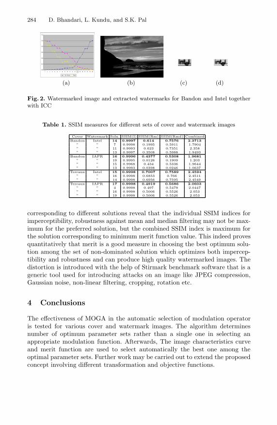
284 D. Bhandari, L. Kundu, and S.K. Pal
(a) (b) (c) (d)
Fig. 2. Watermarked image and extracted watermarks for Bandon and Intel togetherwith ICC
Table 1. SSIM measures for different sets of cover and watermark images
Cover Watermark Soln. SSIM(I) SSIM(Rm) SSIM(Rmd) CombinedBandon Intel 14 0.9997 0.614 0.7576 2.3713
” ” 7 0.9998 0.1995 0.5911 1.7904” ” 11 0.9993 0.623 0.7351 2.358” ” 13 0.9997 0.3508 0.5988 1.9493
Bandon IAPR 16 0.9996 0.4377 0.5308 1.9681” ” 19 0.9995 0.0126 0.1909 1.203” ” 15 0.9968 0.434 0.5336 1.9644” ” 13 0.9993 0.0398 0.0246 1.0637
Terraux Intel 15 0.9998 0.7007 0.7589 2.4594” ” 16 0.9998 0.6853 0.766 2.4511” ” 14 0.9998 0.6956 0.7595 2.4549
Terraux IAPR 17 0.9998 0.4919 0.5686 2.0603” ” 4 0.9998 0.497 0.5479 2.0447” ” 16 0.9998 0.5006 0.5526 2.053” ” 19 0.9998 0.5006 0.5526 2.053
corresponding to different solutions reveal that the individual SSIM indices forimperceptibility, robustness against mean and median filtering may not be max-imum for the preferred solution, but the combined SSIM index is maximum forthe solution corresponding to minimum merit function value. This indeed provesquantitatively that merit is a good measure in choosing the best optimum solu-tion among the set of non-dominated solution which optimizes both impercep-tibility and robustness and can produce high quality watermarked images. Thedistortion is introduced with the help of Stirmark benchmark software that is ageneric tool used for introducing attacks on an image like JPEG compression,Gaussian noise, non-linear filtering, cropping, rotation etc.
4 Conclusions
The effectiveness of MOGA in the automatic selection of modulation operatoris tested for various cover and watermark images. The algorithm determinesnumber of optimum parameter sets rather than a single one in selecting anappropriate modulation function. Afterwards, The image characteristics curveand merit function are used to select automatically the best one among theoptimal parameter sets. Further work may be carried out to extend the proposedconcept involving different transformation and objective functions.

Optimal Parameter Selection for Image Watermarking Using MOGA 285
Acknowledgements
Authors sincerely acknowledge Prof. Malay K. Kundu of MIU, Indian StatisticalInstitute for constructive discussion and suggestion. Sankar K. Pal acknowledgesthe J. C. Bose National Fellowship of the Government of India.
References
1. Ruanaidh, J.J.K.O., Pun, T.: Rotation, translation and scale invariant digital im-age watermarking. In: Proceedings of the International Conference on Image Pro-cessing, Santa Barbara, California, October 1997, vol. 1, pp. 536–539 (1997)
2. Bhandari, D., Murthy, C.A., Pal, S.K.: Image enhancement using multi-objectivegenetic algorithms. In: Chaudhury, S., Mitra, S., Murthy, C.A., Sastry, P.S., Pal,S.K. (eds.) PReMI 2009. LNCS, vol. 5909, pp. 309–314. Springer, Heidelberg (2009)
3. Ekstrom, M.P.: Digital image processing techniques. Academic Press, New York(1984)
4. Hansen, M.P., Jaszkiewicz, A.: Evaluating the quality of approximations to the non-dominated set. Technical Report Technical Report IMM-REP-1998-7, Institute ofMathematical Modelling, Technical University of Denmark (1998)
5. http://www.cl.cam.ac.uk/fapp2/watermarking
6. http://www.ece.uwaterloo.ca/z70wang/research/ssim/
7. Huang, H.C., Pan, J.S., Huamg, Y.H., Huang, K.C.: Progressive watermarkingtechniques using genetic algorithms. Circuits, Systems and Signal Processing 8,58–68 (2007)
8. Katzenbeisser, S., Petitcolas, F.A.P.: Information hiding techniques for steganog-raphy and digital watermarking. Artech House Publishers (2000)
9. Maity, S.P., Kundu, M.K.: Genetic algorithms for optimality of data hiding indigital images. Soft Computing 13(4), 361–373 (2009)
10. Schilling, D.L., Pickholtz, R.L., Millstein, L.B.: Theory of spread spectrumcommunications-a tutorial. IEEE Transactions on Communications 30(5), 855–884(1982)
11. Srinivas, N., Deb, K.: Multiobjective function optimization using nondominatedsorting genetic algorithms. Evolutionary Computation 2(3), 221–248 (1995)
12. Gruhl, D., Bender, W., Morimoto, N.: Techniques for data hiding. In: Proceedingsof the SPIE 2420, Storage and Retrieval for Image and Video Databases III, pp.164–173 (1995)
13. Wang, Z., Bovik, A.C., Sheikh, H.R., Simoncelli, E.P.: Image quality assessment:From error visibility to structural similarity. IEEE Transactions on image process-ing 13(4), 600–612 (2004)
14. Xia, X.G., Boncelet, C.G., Arce, G.R.: A robust digital image watermarkingmethod using wavelet-based fusion. In: Wavelet Transform Based Watermark forDigital Images, vol. 3, pp. 497–511. Optics Express (1998)

Hybrid Contourlet-DCT Based Robust Image
Watermarking Technique Applied to MedicalData Management
Sudeb Das and Malay Kumar Kundu
Machine Intelligence Unit, Indian Statistical Institute, Kolkata 700 108, [email protected], [email protected]
Abstract. This paper describes a non-blind, imperceptible and highlyrobust hybrid Medical Image Watermarking (MIW) technique for a rangeof medical data management issues. The method simultaneously ad-dresses medical information security, content authentication, safe archiv-ing and controlled access retrieval. We propose the use of ContourletTransform (CLT) followed by the Discrete Cosine Transform (DCT) toachieve higher robustness and imperceptibility. Experimental results andperformance comparisons confirm the effectiveness and efficiency of theproposed scheme.
Keywords: Watermarking, Content Authentication, Data integrity,Contourlet Transform.
1 Introduction
The rapid and significant growth of the information and communication tech-nologies has changed the medical data management systems immensely. Themodern integrated health-care delivery systems (such as Hospital ManagementSystems (HISs), Picture Archiving and Communication Systems (PACS) etc.)provide easier access, effective manipulation and efficient distribution of medicaldata. On the other hand these advances have resulted in new risks of inappro-priate use of medical information, due the ease with which digital data can beaccessed and manipulated. Therefore, we need a system for effective storage,transmission, controlled manipulation and access of medical data keeping itsauthenticity, integrity and confidentiality intact [1].
Many MIW techniques have been proposed by various researchers. A spatialdomain technique was proposed by Zain et al. [2] to improve the security of med-ical images by involving the ability to detect tamper and subsequently recoverthe images. A Region of Interest (ROI) lossless MIW technique with enhancedsecurity and high payload embedding in the spatial domain was proposed byKundu et al. in [3]. Chao et al. [4] proposed a DCT based data hiding scheme,capable of hiding EPR in the quantized DCT coefficients of an image. Wu et al.[5] proposed two schemes based on Modulo 256 and DCT, for tamper detectionand recovery purpose. Recently few Discrete Wavelet Transform (DWT) based
S.O. Kuznetsov et al. (Eds.): PReMI 2011, LNCS 6744, pp. 286–292, 2011.c© Springer-Verlag Berlin Heidelberg 2011
Watermarking Technique Applied to Medical Data Management 287
MIW methods have been proposed [6][7][8] by various researchers. Most of theprevious researches have concentrated on preserving the resolution of the med-ical images after watermark embedding, regardless of testing the robustness ofthe schemes against different attacks. Moreover, most of the conventional wa-termarking schemes are semi-robust in nature. They can resist either the signalprocessing attacks destroying the high frequency (HF) components of the image,or the signal processing operations in which the low frequency (LF) componentsof the image is altered.
To overcome these problems, we propose a hybrid CLT-DCT based MIWtechnique to hide Electronic Patient Record (EPR), Doctor’s Identification Code(DIC) and Indexing Keyword (INDX) in the medical image. The confidentialityof the EPR is improved by embedding the data in the image. DIC works as asource authenticator and INDX serves as a querying keyword for use in medicalimage databases for effective image retrieval. In addition to that, both the stor-age and transmission bandwidth requirements as well as the possibility of EPRdetachment are reduced. In the proposed method, watermark’s DCT coefficientsare inserted into the DCT coefficients of the CLT transformed low pass versionof the original image. Due to the special transform structure of Laplacian Pyra-mid (LP) [9], the DCT coefficients of the watermark are likely to be spread outinto all subbands when we reconstruct the watermarked image. As a result theproposed technique is expected to be robust to various attacks resulting fromboth the signal processing operations which affect the HF or the LF componentsof the image.
The organization of the paper is as follows: in Section 2 we briefly describe theCLT. We outline in Section 3 the proposed watermark embedding and extractionalgorithms. Experimental results and comparisons are presented in Section 4 andwe draw conclusion in Section 5.
2 Contourlet Transform (CLT)
The major drawback of DWT in two dimensions is their limited ability in cap-turing directional information. In light of this, Do and Vetterli [9][10] developedthe CLT based on an efficient two-dimensional multiscale and directional filterbank (DBF). CLT not only possess the main features of DWT, but also offer ahigh degree of directionality and anisotropy. It allows for different and flexiblenumber of directions at each scale, while achieving nearly critical sampling. Inaddition, CLT uses iterated filter banks, which makes it computationally efficient(O(N) operations for an N-pixels image).
CLT gives a multiresolution, local and directional expansion of image usingPyramidal Directional Filter Bank (PDFB). The PDFB combines LP whichcaptures the point discontinuities, with a DFB which links these discontinuitiesinto linear structures. LP is a multiscale decomposition of L2(R2) into series ofincreasing resolution subspaces which are orthogonal complements of each otheras follows:

288 S. Das and M.K. Kundu
L2(R2) = Vj0 ⊕ (−∞⊕
j=J0
Wj) (1)
An l-level DFB generates a local directional basis for l2(Z2) that is composedof the impulse response of the DFBs and their shifts. In CLT, the directionalfilter is applied to the detail subspace Wj . This results in a decomposition of Wj
into 2lj subspaces at scale 2j .
Wj =2lj−1⊕
k=0
Wljj,k (2)
Fig. 1.(a) shows the flowchart of CLT for a 512 × 512 image. A DFB is de-signed to capture the high frequency content like smooth contours and directionaledges. This DBF is implemented by using a k-level binary tree decompositionthat leads to 2k subbands with wedge shaped frequency partition as shown inFig. 1.(b).
(a) (b)
Fig. 1. (a) Flowchart of CLT for a 512 × 512 image. (b) Frequency partitioning (k =3, 2k = 8) wedge shaped frequency subbands.
3 Proposed Scheme
The watermark embedding and extraction algorithm is described here.
3.1 Watermark Embedding
The salient steps of the watermark embedding process are as follows:
1. Apply CLT on the original image I.2. Divide the coefficients of the low pass subband (ILPS) of the transformed I
into 8 × 8 non-overlapping blocks.3. Perform DCT to each block of ILPS to get DCT ILPS .4. Encrypt the EPR by Advanced Encryption Standard (AES) method using
a secret key KS to get EPRENCRY .

Watermarking Technique Applied to Medical Data Management 289
5. Concatenate DIC, INDX , EPRENCRY and represent the resultant stringto its binary representation as WMBIN .
6. Apply BCH error correcting code to WMBIN to get WMBCH .7. Reshape WMBCH as a 1D-binary string (WMBS) and scatter its bits using
the function given below:
f(x) = px mod n + 1 (3)
where,n = size of the subband ILPS ;p = secret prime number ε [1, n];x = bit position in WMBS and x ε [1, length(WMBS)];
8. Reshape the resultant string in a matrix of equal size as ILPS to get the finalwatermark payload WMFIN .
9. Divide WMFIN into 8 × 8 non-overlapping blocks, and perform DCT toeach block to get DCTWM .
10. Let, a coefficient of the matrix DCT ILPS , is represented by Y (x, y), andW (x, y) represents a coefficient of the matrix DCTWM . Then, perform ad-ditive watermarking operation:
Y ′(x, y) = Y (x, y) + αW (x, y) (4)
where,Y ′(x, y) = coefficients of the reconstructed matrix DCT ′ ILPS ;α = watermarking strength factor.
11. Perform Inverse DCT on DCT ′ ILPS , to get the modified I ′LPS .12. To get the watermarked image I∗, apply Inverse CLT on the I ′
LPS , alongwith other non-modified directional subbands.
3.2 Watermark Extraction
The proposed watermarking scheme is non-blind, which means we need the orig-inal image during the extraction process. The steps of the extraction process areas follows:
1. Apply CLT on I and I∗ (possibly attacked) with the same decompositionconfiguration of the embedding process.
2. Divide the coefficients of the low pass subbands (ILPS and I∗LPS respectively)
of the transformed I and I∗ into 8 × 8 non-overlapping blocks.3. Get DCT ILPS and DCT I∗
LPS by performing DCT to each block of ILPS
and I∗LPS respectively.4. Let, a coefficient of the matrix DCT ILPS , is represented by Y (x, y), and
Y ∗(x, y) represents a coefficient of the matrix DCT I∗LPS . Then, to get one
coefficient W ′(x, y) of the reconstructed DCT watermark DCTWM ′ performthe following operation:
W ′(x, y) = (Y ∗(x, y) − Y (x, y))/α (5)

290 S. Das and M.K. Kundu
5. Perform the Inverse DCT on DCTWM ′ , to get the reconstructed watermarkWM ′.
6. Reshape WM ′ as a binary string and rearrange the bits to their originalpositions using the equation 3 to get WM ′
BCH .7. Get WM ′
BIN by applying BCH decoding procedure on WM ′BCH .
8. Transform WM ′BIN to its original format and separate DIC, INDX , and
EPRENCRY .9. Decrypt EPRENCRY using the same secret key KS to get the original EPR.
4 Experimental Results and Comparisons
4 grayscale (8 bpp) medical images of different modalities (CT, MRI, USG), ofsize 512× 512 were used in the experiments. The DIC and INDX consist of 20(20× 7 = 140 bits) and 14 (14× 7 = 98 bits) ASCII characters respectively. Thesize of the encrypted EPR was 1152 bits. After applying BCH(255,139,15) thesize of the watermark was 2550 bits. After three level CLT [2,4,8] of the imagewith ‘9-7’ pyramid filter and ‘pkva’ directional filter, the size of the low passsubband was 64× 64. We used p = 23 in the equation 3. The value of α was setto 30 after lots of experiments.
We used Peak Signal-to-Noise Ration (PSNR) to measure the distortion pro-duced after watermark embedding. Mean Structural SIMilarity index (MSSIM)was used to measure the similarity between the original image and the water-marked image. To prove the authenticity of the extracted watermark we usedNormalized Correlation (NC) coefficient and Bit Error Rate (BER).
Table 1. shows the PSNR, MSSIM, NC and BER values in attack free case.The result shows that the watermark is retrieved successfully without any er-rors. Fig. 2. shows the effect of watermark embedding in the medical images.The results show that there is no visual difference between the original and thewatermarked images.
The results (for abdomenCT image) in the Table 2. show that the proposemethod is robust against various image processing attacks. It also shows thevisual and structural difference between the watermarked and the attacked imagein terms of PSNR and MSSIM.
Comparisons with [7] and [8] reveals that, these methods are more impercep-tible (in terms of PSNR), but less robust than our scheme. Specifically, thesemethods can only survive JPEG compression attack, even that also to a limited
Table 1. Results of Attack Free Case
Image PSNR MSSIM NC BER
abdomeCT 41.5895 0.8745 1.0000 0
cthead 41.5713 0.9567 1.0000 0
mriBrain 41.5157 0.9747 1.0000 0
usg 41.4776 0.9383 1.0000 0

Watermarking Technique Applied to Medical Data Management 291
Fig. 2. Original images (above) and their corresponding watermarked images (below)
Table 2. Robustness Against Various Attacks
Attacks Parameters NC BER PSNR MSSIMMean Filtering Window size = 3 × 3 1.0000 0.0000 31.8707 0.9434
Median Filtering Window size = 3 × 3 1.0000 0.0000 34.7341 0.9555
Salt & Pepper Noise Noise density = 0.005 1.0000 0.0000 26.9014 0.8790
Cropping 315 × 27 pixels 1.0000 0.0000 20.6878 0.9588
Resize 256 × 256 pixels 1.0000 0.0000 33.2382 0.9525
Bit-Plane Removal LSB-1 1.0000 0.0000 52.1812 0.9936
Sharpening 65 1.0000 0.0000 29.1512 0.9125
JPEG Quality Factor = 25 1.0000 0.0000 34.5269 0.8819
quality factor (< 50). Whereas, our scheme can survive JPEG compression at-tack up to 25 quality factor. In [7] only the ROI of the image can be embedded,but no EPR or DIC or INDX. Comparison with [6] shows that, our method ismore imperceptible (in terms of PSNR) and also more robust. Also the use ofEPR encryption, scattering of bits in the embedding process makes our methodmuch more secure than the methods mentioned above.
5 Conclusions
We have presented a non-blind, highly robust watermarking scheme applied tomedical images with good imperceptibility and enhanced security. Our schemecan be used for different medical image modalities. The experimental resultsindicate that the proposed scheme is feasible and given its relative simplicity, itcan be applied to the medical images at the time of acquisition to serve in manymedical applications concerned with authenticity, integrity and confidentiality.
In future research, we will try to enhance our algorithm by making it blind,as well as, we will try to embed the watermark such that, it cause less visualdegradation and better extraction accuracy.
292 S. Das and M.K. Kundu
References
1. Coatrieux, G., Maitre, H., Sankur, B., Rolland, Y., Collorec, R.: Relevance ofwatermarking in medical imaging, pp. 250–255 (2000)
2. Zain, J.M., Fauzi, A.R.M.: Medical image watermarking with tamper detectionand recovery. In: Proc. 28th IEEE EMBS Annual International Conference, pp.3270–3273 (2006)
3. Kundu, M.K., Das, S.: Lossless roi medical image watermarking technique withenhanced security and high payload embedding. In: Proc. IEEE International Con-ference on Patter Recognition (ICPR), pp. 1457–1460 (2010)
4. Chao, H., Hsu, C., Miaou, S.: A data-hiding technique with authentication, inte-gration, and confidentiality for electronic patient records. IEEE Trans Inf. Technol.Biomed. 1, 46–53 (2002)
5. Wu, J.H.K., Chang, R.F., Chen, C.J., Wang, C.L., Kuo, T.H., Moon, W.K., Chen,D.R.: Tamper detection and recovery for medical images using near-lossless infor-mation hiding technique. Journal of Digital Imaging 21, 59–76 (2008)
6. Manasrah, T., Al-Haj, A.: Management of medical images using wavelets-basedmulti-watermarking algorithm. In: Proc. Int. Conf. Innovations in InformationTechnology, pp. 697–701 (2008)
7. Lee, H.K., Kim, H.J., Kwon, K.R., Lee, J.K.: Roi medical image watermarkingusing dwt and bit-plane. In: Proc. Asia-Pacific Conf. Communica, pp. 512–515(2005)
8. Giakoumaki, A., Pavlopoulos, S., Koutsouris, D.: Multiple image watermarking ap-plied to health information management. IEEE Trans. on Information Technologyin Biomedicine 10, 722–732 (2006)
9. Do, M.N., Vetterli, M.: Contourlets. In: Welland, G.V. (ed.) Beyond Wavelets,Academic Press, New York (2003)
10. Do, M.N., Vetterli, M.: The contourlet transform: An efficient directional multireso-lution image representation. IEEE Transactions on Image Processing 14, 2091–2106(2005)

Accurate Localizations of Reference Points in a
Fingerprint Image
Malay Kumar Kundu and Arpan Kumar Maiti
Center for soft computing Research, Indian Statistical Institute, [email protected], [email protected]
Abstract. Reference points play important role in the field of finger-print recognition. It is mainly used for fingerprint classification and fin-gerprint matching. There are many methods proposed for fingerprintreference point detection like Poincare Index technique, Direction curva-ture technique etc. The purpose of this paper is to detect the referencepoints considering the uncertainty for imperfection of fingerprint refer-ence point position.
1 Introduction
Biometric Application,Fingerprint, has taken part a major role to identify aparticular person uniquely. We can analyze the fingerprint from global and localperspective.From local perspective we concentrate on minutiae like bifurcationpoint,trifurcation,ridge ending etc. At global level ,there are some unique land-marks of fingerprint,where the ridge curvature is higher than other areas andthe orientation changes rapidly. They are commonly known as core and delta[4]which are shown in Fig1(a) and they are used as a reference point. Each fin-gerprint should have the local features and may or may not have the globalfeature. The number of core and delta point differs in different type of finger-print. There are several techniques available for singular point detection. Mostof the techniques developed on the basis of orientation field of the image. Thepoincare index method(PI) one of the commonly used method for reference pointdetection[1][7]. This method is efficient but very much sensitive to noise as theorientation deviation caused by image imperfection that effects the computationof PI. Another method is to detect the reference point by searching the curvaturepoint from the orientation image[6][8][3].
The main problem of all such approaches is the uncertainty presents in theprocess of detection of the exact location of reference points. Though it is easyto detect the approximate region where reference point exists but it is difficultto get a unique point as a reference one. In this paper we have proposed amethod where some template is to be used to detect the reference points usingstrength of similarity from which the exact (single) point may be detected fromthe approximate core and delta region using fuzzy reasoning.
Organization of the paper is as follows. The estimation of direction field andreference points are presented in section 2.1 and 2.2 The false reference Point
S.O. Kuznetsov et al. (Eds.): PReMI 2011, LNCS 6744, pp. 293–298, 2011.c© Springer-Verlag Berlin Heidelberg 2011

294 M.K. Kundu and A.K. Maiti
(a) FingerprintReference Point
(b) Originalimage
(c)Orientation
image
Fig. 1. (a)Fingerprint Reference point (b)Original finger print image (c) field of Fin-gerprint image
removal technique is described in section 3. In section 4,A technique for identifi-cation of finer core point from core region is described. The experimental resultsand future works are given in section 5 and 6.
2 Proposed Method to Identify Reference Points
2.1 Formation of Orientation Image
Before going to minutiae extraction,an orientation field flow map is computed.The input image is subdivided into number of blocks of equal size and dominantridge gradient direction is computed for each block. The average direction ofall ridges represents the dominant direction of each block. Same algorithm isrepeated for each block. So the image is scaled down by the size of factor w ifWe assume that the size of each block is w×w. All possible directions should getconverted only into eight discrete directions in the range of 90 degree to -67.5degree[9][2]. The Direction angle θ(i,j) is representing the dominant direction ofthe block (i,j). Now the reduced image is represented as D(i, j) and its positionis represented by Dij . The main steps to calculate the orientation of each blockis as follows.1)Divide the fingerprint image into non overlapping blocks of size w × w.2)Compute the gradient δx(i, j) and δy(i, j) of each pixel (i,j) corresponding tothe Horizontal and vertical direction.The gradient operator used here is Sobeloperator for simplicity.3)Estimate the orientation of each block (i,j) by averaging the square gradientsas follows.
Vy(i, j) =i+w/2∑
u=i−w/2
j+w/2∑
v=j−w/2
2δx(u, v)δy(u, v) (1)
Vx(i, j) =i+w/2∑
u=i−w/2
j+w/2∑
v=j−w/2
(δ2x(u, v) − δ2
y(u, v)) (2)

Accurate Localizations of Reference Points in a Fingerprint Image 295
θ(i, j) = (1/2)tan−1(Vy(i, j)/Vx(i, j)) (3)
The original Fingerprint image and its direction image is shown in Fig 1(a),(b).
2.2 Reference Point Detection
The Poincare index method and the modified Poincare Index Method are themost popular method to detect the singular points in the fingerprints. By usingthis method the core point,delta points and virtual core point for whorl type areextracted on the basis of gradient differences among the adjacent blocks[1][7].But it has been shown that reference point detection is considerably difficult forlow quality image and the image containing noise. This may cause the faultydetection of reference point.
(a) Coremask
(b) whorlmask
(c) Deltamask
Fig. 2. Different mask figure a)Core b)Whorl)delta
To overcome this problem,besides the gradient difference method proposedin PI method additionaly We have used block based matching technique wherenumber of blocks are used which depicts the different kind of reference pointpattern. This hugely improved the performance of fingerprint reference pointdetection methodology. The template masks, CoreM (i, j),WhorlM (i, j) andDeltaM(i, j) in fig2 are defined as a convolution mask for calculating similaritymeasurement strength of each pattern in the Direction image. Initially We con-sider three empty sets for the core,whorl and delta point ,let it say SC ,SW ,SD.
Each point of direction image D(i, j) is checked with all the template mask andcorrelation membership value or similarity measurement strength is calculatedusing the equation (4). As the convolution template are asymmetric the exactmid point or near mid point is chosen for calculating the correlation membershipvalue,let say the point index as midi and midj .
μC(Dij)=MH∑
u=−1
MW∑
v=−1
1 − |(D(i+u)(j+v)−CoreM (midi + u)(midj + v))|δk
(4)
μC(Dij) = μC(Dij)/NC (5)
where MH is the height of the Mask,MW is Width of the Mask,δk is maximumpossible phase angle difference,here 157.5(90 to -67.5) and NC is No of consid-erable points in the Mask.

296 M.K. Kundu and A.K. Maiti
Using the above mentioned equation,correlation membership value is calcu-lated using all the mask and say it μC(Dij),μW (Dij) and μD(Dij) for core,whorltype and delta. Now a cutoff value is decided to get the correct point into theset SC ,SW , SD using the equation (6).
SC = Di,j : μC(Di,j) > μCT SW = Di,j : μW (Di,j) > μWT SD = Di,j : μD(Di,j) > μDT (6)
where μCT ,μWT and μDT are the membership cut off value for core point,whorltype and Delta Point. The above mentioned approach is continued in reverseimage to check any other reference point from the opposite direction using thesame algorithm.
3 False Reference Point Detection and Removal
All the candidate points which has been detected in the set SC ,SW and SD arenot the correct reference point. In this scenario it has been shown that if Wetake the help of poincare indexing method, it will remove the unnecessary corepoint and delta point from the set SC and SD.
From the experiment It has been shown that there may be some points inthe set which are neighbor of each other. Multiple reference points can not bepresent within the neighborhood position so the points are to be removed fromthe set. In this scenario,Lower most Horizontal line of the Image has been takenas a base line and the candidate point having smallest distance from the baseline considered as reference point.
The virtual core point(Whorl type) is a special type of point where two ex-treme curvature point exist above and below of the whorl pattern. As whorlpoint is being detected separately so at that particular case,these two extremecurvature points marked as a core point are removing from the set SC usingequation (7) and the new set is formed SNew
C . Finally We can draw a hypothet-ical line joining these two points and center of this line can be assumed as avirtual core point for whorl type which is shown in Fig 3(a).
SNewC = SC − x (7)
If(x ∈ SC and y ∈ xn8 and y ∈ SW ), Check ∀x ∈ SC
where xn8 is the set of 8 neighbor points of x.
4 Identification of Finer Point from Core Region
Its a challenge to identify the exact core point position from the identified coreregion. It is found that the exact core point is the sharpest corner situated inthe innermost ridge.To identify a corner point We have estimated some localshape parameters gradient,symmetry and straightness for this purpose. An ideal

Accurate Localizations of Reference Points in a Fingerprint Image 297
corner point should have high gradient value,high reflective symmetry and lowlevel straightness in a local neighborhood of pixels[5].Cornerness is checked usingthe table in Fig3(b)for decision making. Each parameter value of the core regionpoints are calculated and the range between the extreme low and extreme highvalue is equally subdivided into three range low,medium and high. An Exampleof finer core points (single pixel or cluster of very few pixels) detection usingproposed method and core region detection using poincare method is shown inFig4(e) and (d).
(a) Virtual core point (b) Cornerness Decision making
Fig. 3.
(a) Originalimage
(b) zoomingcore region
(c)Orientation
image
(d) Poincaremethod
(e) Finer core Point
Fig. 4. Finer core point Identification
5 Experimental Results
To evaluate the performance of this algorithm, We have used the testing databaseFVC 2000 (http://bias.csr.unibo.it/fvc2000/databases.asp) for all type of finger-print Image.The orientation image is formed using 8 × 8 block. The Similaritymeasurement strength cut off values are decided .8,.85 and .85 for μCT ,μWT
and μDT respectively considering the effect for large number of images.SomeFingerprint Image and its reference points are shown in Fig 5.

298 M.K. Kundu and A.K. Maiti
(a) (b) (c) (d) (e) (f)
Fig. 5. Result Image with Core,Whorl and Delta Point
6 Conclusion
In this paper we have tried to overcome the uncertainty during the identificationof exact reference point location using decision making rules. But We expectthat any soft computing tool like fuzzy set theory can play important role formodeling such type of uncertainty and that is being persuaded currently.
References
1. Huang, T., Liu, C., Lin, J., Li, C., Kuo, T.: A novel scheme for fingerprint identifica-tion. In: The 2nd Canadian Conference on Computer and Robot Vision, Proceedings,pp. 392–396 (2005)
2. Jayadevan, R., Kulkarni, J.V., Mali, S.N., Abhyankar, H.K.: A new ridge orienta-tion based method of computation for feature extraction from fingerprint images.Transactions on Engineering, Computing and Technology (2007)
3. Kekre, H.B., Bharadi, V.A.: Fingerprint’s core point detection using orientationfield. In: International Conference on Advances in Computing, Control, Telecom-munication Technologies, ACT 2009, pp. 150–152 (2009)
4. Kekre, H.B., Bharadi, V.A.: Article: Fingerprint core point detection algorithmusing orientation field based multiple features. International Journal of ComputerApplications 1(15), 97–103 (2010)
5. Law, T., Yamada, K., Shibata, D., Nakamura, T., He, L., Itoh, H.: Edge extractionusing fuzzy reasoning. In: Pal, S.K., et al. (eds.) Soft computing for image processing,vol. 42, pp. 44–78 (2000)
6. Mohammadi, S., Farajzadeh, A.: Fingerprint reference point detection using ori-entation field and curvature measurements. In: IEEE International Conference onIntelligent Computing and Intelligent Systems, ICIS 2009, vol. 4, pp. 25–29 (2009)
7. Ohtsuka, T., Watanabe, D., Tomizawa, D., Hasegawa, Y., Aoki, H.: Reliable de-tection of core and delta in fingerprints by using singular candidate method. In:IEEE Computer Society Conference on Computer Vision and Pattern RecognitionWorkshops, CVPRW 2008, pp. 1–6 (2008)
8. Yin, Y., Weng, D., Li, H., Ma, W.: A new robust method of singular point de-tection from fingerprint. In: International Symposium on Information Science andEngieering, vol. 2, pp. 330–334 (2008)
9. Zhang, W., Wang, Y.: Singular point detection in fingerprint image. In: The 5thAsian Conference on Computer Vision (2002)

Adaptive Pixel Swapping Based Steganography
Reducing Embedding Noise
Arijit Sur1, Piyush Goel2, and Jayanta Mukhopadhyay2
1 Department of Computer Science and Engineering,Indian Institute of Technology, Guwahati-781039, India2 Department of Computer Science and Engineering,
Indian Institute of Technology, Kharagpur-721302, [email protected], piyush,[email protected]
Abstract. In this paper1, a block based steganographic algorithm isproposed where embedding is done by swapping two pixels within theblock such that resulting additive noise can be adaptively controlledby using a prescribed threshold. The proposed algorithm is used to re-duce the extra additive noise which is the main drawback of a existingPSSA algorithm [6]. Regarding the steganographic security, the proposedsteganographic scheme inherently preserves first order image statisticssuch as image histogram and thus remains undetectable against any his-togram based spatial domain steganalytic attacks. Experimental resultsshow that the proposed adaptive scheme clearly outperforms the PSSAalgorithm [6] against additive noise based blind attacks.
1 Introduction
Steganography is the art of hiding information in an innocent looking cover ob-jects and thus visual and statistical undetectability is one of the major concernsin the steganographic security. In recent steganalytic literature, a major numberof algorithms (e.g. [1][2]) are based on first order image statistics. The mainproblem of restoring image statistics is that an extra amount of additive noise isbeing added during restoration. This extra additive noise makes those algorithmsmore vulnerable against additive noise based blind attacks like WAM [3]. It iswell known that the chance of detection is substantially reduced if embeddingis done adaptively. In this paper, we have consider an existing pixel swappingbased spatial domain embedding scheme [6] which can inherently restores imagehistogram and thus can resist histogram based targeted attacks. The main draw-back of the PSSA algorithm [6] is that it essentially adds a substantial amountof extra additive noise due to the restoration process compared to that of LSBmatching type of algorithms. In this paper, we have proposed a new AdaptivePixel Swapping based Steganographic Algorithm (APSSA) algorithm by intro-ducing a block based local adaptive threshold such that amount of noise added
1 The first author gratefully acknowledge the support received from Infosys Technolo-gies Ltd., Bangalore, under the Infosys Fellowship Award.
S.O. Kuznetsov et al. (Eds.): PReMI 2011, LNCS 6744, pp. 299–304, 2011.c© Springer-Verlag Berlin Heidelberg 2011

300 A. Sur, P. Goel, and J. Mukhopadhyay
(in a block) depends on certain local (within the block) image statistics. It isexperimentally shown that proposed scheme has similar performance with PSSAagainst several recent targeted steganalysis attacks while the proposed adaptivemodification made APSSA more secure than PSSA scheme [6] against additivenoise based attacks like WAM [3]. The rest of the paper is organized as follows.The proposed encoding and decoding algorithm are described in Sec. 2. In Sec.3, steganalytic security of the proposed scheme is discussed. The paper will beconcluded in Sec. 4.
2 Proposed Scheme
In this paper, a block based pixel swapping algorithm is proposed which is anadaptive improvement over the pixel swapping scheme proposed in [6]. Firstly,the image is divided into non overlapping blocks with a fixed dimension. A singlebit is embedded in a block. Let I be the gray scale cover image. Let Ik(α) be theintensity value of a fixed location α in the kth block of the image I. Ik(β) andIk(γ) are another two block locations such that β and γ are defined as follows:
β = argmaxm∈IK (IK(m) < μk) (1)
γ = argminm∈IK (IK(m) > μk) (2)
where IK = Ik − Ik(α). So Ik(β) is a block element other than Ik(α) which isthe maximum value just less than μk. Similarly Ik(γ) is a block element otherthan Ik(α) having minimum value just greater than μk.
The embedding rule is constructed as follows:
bit embedded =
⎧⎨
⎩
1 if Ik(α) > μk
0 if Ik(α) < μk
(3)
where μk = mean of the kth block. In other words, if Ik(α) is greater than themean of kth block μk, the embedded bit is taken as 1; on the other hand if Ik(α)is less than μk, the embedded bit is taken as 0.
A bit is embedded in the kth block if following suitability condition is true forthat block
|Ik(α) − μk| < τ (4)
where τ is the prescribed threshold.For a suitable block (say bk), the present secret bit (Spresent) and Ik(α) are
checked according to the embedding rule. If the embedding condition [(Spresent =1) & (Ik(α) > μk)] is satisfied, no operation is needed to embed the data bit,otherwise Ik(α) is swapped with Ik(β) or Ik(γ) according to Spresent. A data bitis embedded if suitability condition is satisfied, otherwise no bit is embedded. Inlater case, swapping is needed to mark the corresponding block unsuitable forembedding.

Adaptive Pixel Swapping Based Steganography Reducing Embedding Noise 301
This amounts to addition of extra noise. This particular situation hap-pens when both the conditions |Ik(α) − μk| < τ and |Ik(β) − μk| > τ [or,|Ik(α) − μk| < τ and |Ik(γ) − μk| > τ ] are true. It is experimentally foundthat the probability of occurrences of these situations is very low. This is be-cause Ik(β) has the lowest intensity value greater than μk of the block and Ik(γ)has the highest intensity value less than μk of that block. Again for a slightlyhigher value of τ the situation becomes more rare. Since the total noise addeddue to this extra swapping is almost negligible, it is not considered in the the-oretical computation of noise. There is an obvious trade off between payloadand embedding noise. For a relatively higher payload, embedding noise wouldbe relatively high. However when the block size is greater than two, the choice ofpixels used for swapping can be possible. This adaptiveness makes the APSSAscheme more secure than PSSA [6] scheme reducing the embedding noise. Astep by step algorithm is given below:
2.1 Embedding Algorithm
Algorithm. Adaptive Pixel Swapping based Steganographic Algorithm(APSSA)Input: Cover Image I, Secret Bit Sequence S, present secret bit is representedby Spresent
Input Parameters: Shared secret seed for generating pseudorandom sequence,Threshold (τ)Output: Stego Image Is
1. The Cover image I is divided into non over lapping blocks of N pixels.2. Blocks are arranged with a pseudorandom sequence using the shared secret
seed.3. For any block, (let kth block is denoted as Ik), a fixed block location is
determined. Let it be denoted by Ik(α). Another two block elements aredefined as Ik(β) and Ik(γ) where β = argmaxm∈IK (IK(m) < μk) andγ = argminm∈IK (IK(m) > μk) where μk is the mean of the block Ik andIK = Ik − Ik(α). Let the variable done act as a flag denoting, whether theblock is used for embedding or not.
4. done = 0
if 0 < |Ik(α) − μk| < τif ( Spresent == 0)
if Ik(α) > μk)swap (Ik(α), Ik(β))if |(Ik(β) − μk)| > τ
done = 0;else
done = 1;else
done = 1;

302 A. Sur, P. Goel, and J. Mukhopadhyay
elseif Ik(α) < μk)
swap (Ik(α), Ik(γ))if |(Ik(γ) − μk)| > τ
done = 0;else
done = 1;else
done = 1;if done == 1
spresent=next secret bit
5. Next block is taken and repeat steps 3 and 4 until either the secret sequence(S) is exhausted or all embedding blocks have been used.
6. Using above steps elements of S embedded into I to get stego image Is.
End. Adaptive Pixel Swapping based Steganographic Algorithm (APSSA)
2.2 Extraction Algorithm
The extraction algorithm is quite simple. The pseudorandom sequence of blocksis regenerated at decoder with the help of the shared secret seed. A block (sayIk) is not considered for extraction if |Ik(α) − μk| ≥ τ or |Ik(α) − μk| = 0.Otherwise, for any block if Ik(α) > μk, the corresponding secret bit is recoveredas 1 and 0 if Ik(α) < μk. Bit stuffing is used to distinguish between secretsequence and terminator string.
3 Experimental Results
3.1 Reduction of Additive Noise
The main goal of the proposed APSSA scheme is to reduce the additive noisedue to the embedding and restoration process of the embedding. In Figure 1,PSNR between cover and stego images are shown for both the PSSA [6] andthe APSSA scheme. The experiments are done on 100 randomly chosen imagesfrom a never compressed image dataset UCID [4]. In Figure 1, it is observedthat the PSNR between cover and stego images of the proposed APSSA schemeis relatively higher than that of PSSA [6] scheme which implies the reduction ofadditive noise due to adaptive modification.
3.2 Security against Blind Steganalysis
The main drawback of the PSSA [6] algorithm is that it added a substantialamount of extra additive noise during restoration process compared to the algo-rithms similar to the LSBM .

Adaptive Pixel Swapping Based Steganography Reducing Embedding Noise 303
Fig. 1. Comparison of PSNR between Proposed APSSA and PSSA [6] Scheme
For testing the performance of the APSSA algorithm, experiments are con-ducted on a data set of two thousand test images which were divided into twoequal sets of one thousand cover images and one thousand stego images. 1000never compressed images are taken from the UCID [4] as cover images and 1000stego images are generated using the APSSA algorithm. In these experiments, ablock with four pixels is used. It is experimentally found that the payload for thebigger blocks are very less and is mostly undetectable. To evaluate the stegano-graphic security using the proposed scheme, Area under the Receiver OperatingCharacteristic Curve (AROC) and the Detection accuracy (Pdetect) [5] which iscomputed using equations 5 and 6 have been used as the evaluation metrics.
Pdetect = 1 − Perror (5)
Perror =12× PFP +
12× PFN (6)
where PFP , PFN are the probabilities of false positive and false negative respec-tively. A value of Pdetect = 0.5 shows that the classification is as good as randomguessing and Pdetect = 1.0 shows a classification with 100% accuracy.
For the evaluation of the proposed APSSA scheme, Wavelet absolute mo-ment (WAM) steganalyzer [3] is considered as steganalytic attack. In Figure 2,
(a) Emb. rate 0.10 bpp (b) Emb. rate 0.225 bpp
Fig. 2. ROC plot for comparing between APSSA and PSSA [6] against WAM

304 A. Sur, P. Goel, and J. Mukhopadhyay
it is shown that proposed APSSA scheme is relatively less detectable than thePSSA scheme [6] against WAM at the same embedding rates using never com-pressed image dataset as cover image source. Since, the histogram of the imageis kept intact during embedding, proposed adaptive improved scheme remainsundetectable against any histogram based spatial domain steganalytic attackssimilar to the PSSA scheme [6].
4 Conclusion
In this paper, an adaptive improvement over PSSA algorithm [6] is proposedby incorporating a block based local adaptive threshold such that the amountof additive noise can be controlled adaptively using block image statistics. Wehave experimentally shown that the enforced adaptiveness makes the schememore secure than its non adaptive version (PSSA) against additive noise basedsteganalyzers while it maintains same performance as PSSA against targetedattacks since image histogram is kept intact during embedding.
References
1. Ker, A.D.: Steganalysis of LSB matching in grayscale images. IEEE Signal process-ing letters 12(6), 441–444 (2005)
2. Zhang, J., Cox, I.J., Doerr, G.: Steganalysis for LSB Matching in Images with High-frequency Noise. In: Proc. IEEE 9th Workshop on Multimedia Signal ProcessingMMSP 2007, pp. 385–388 (2007)
3. Goljan, M., Fridrich, J., Holotyak, T.: New blind steganalysis and its implications.In: Proceedings of SPIE for Security, Steganography, and Watermarking of Multi-media Contents VIII, vol. 6072, pp. 1–13 (2006)
4. Schaefer, G., Stich, M.: UCID - An Uncompressed Colour Image Database. In: Proc.SPIE, Storage and Retrieval Methods and Applications for Multimedia, vol. 5307,pp. 472–480 (2004)
5. Solanki, K., Sarkar, A., Manjunath, B.S.: YASS: Yet Another SteganographicScheme That Resists Blind Steganalysis. In: Furon, T., Cayre, F., Doerr, G., Bas,P. (eds.) IH 2007. LNCS, vol. 4567, pp. 16–31. Springer, Heidelberg (2008)
6. Sur, A., Goel, P., Mukhopadhyay, J.: A Novel Steganographic Algorithm ResistingTargeted Steganalytic Attacks on LSB Matching. In: Kim, H.-J., Katzenbeisser, S.,Ho, A.T.S. (eds.) IWDW 2008. LNCS, vol. 5450, pp. 199–208. Springer, Heidelberg(2009)
Classification and Quantification of Occlusion
Using Hidden Markov Model
C.R. Sahoo1, Shamik Sural1, Gerhard Rigoll2, and A. Sanchez3
1 School of Information Technology, Indian Institute of Technology, Kharagpur, [email protected], [email protected]
2 Technical University of Munich, Munich, [email protected]
3 Universidad Rey Juan Carlos, Madrid, [email protected]
Abstract. Over the last few years, gait recognition has become an activearea of research. However, one of the shortcomings is lack of a methodfor quantifying occlusion in scenes used for capturing gait of individuals.Occlusion can occur primarily because of two reasons. Firstly, movementof certain body parts of a human being occludes some other body parts ofthe same human, which is called self occlusion and secondly, occlusion ofthe body parts caused by some other human being. The objective of thispaper is to quantify occlusion of different parts of the human body usingHidden Markov Model (HMM) and classify the scene of occlusion as oneof the three cases of occlusion, namely, self occlusion (single individualmoving), occlusion in a crowd moving in same direction and occlusiondue to movement of human beings approaching from opposite direction.We train one HMM for each body part relevant for gait recognition. AnHMM is a statistical representation of probability distribution of a largenumber of possible sequences and in the current context these are thesequences of frames extracted at regular interval from a given video. Thesteps involved in achieving the objective are feature extraction, HMMtraining and finally the classification or hidden state generation.
Keywords: Occlusion, Gait Recognition, Body Part, HMM.
1 Introduction
One of the most active research areas in computer vision, human gait recognitionbroadly deals with detecting, tracking and identifying people from a sequenceof images. Gait recognition has attracted great interest due to its promisingapplications in visual surveillance, with the added advantage of not requiring anyactive participation of the subject whose gait is under consideration. Even lowend cameras with very low resolution provide adequate accuracy in recognition.However, occlusion handling still remains an area of concern [8].
Other than human gait recognition, a number of algorithms have been pro-posed for tracking and motion detection [9, 4]. But none of them quantify oc-clusion. In this paper, we propose a method for quantifying occlusion by using
S.O. Kuznetsov et al. (Eds.): PReMI 2011, LNCS 6744, pp. 305–310, 2011.c© Springer-Verlag Berlin Heidelberg 2011
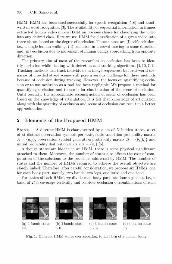
306 C.R. Sahoo et al.
HMM. HMM has been used successfully for speech recognition [5, 6] and hand-written word recognition [3]. The availability of sequential information in framesextracted from a video makes HMM an obvious choice for classifying the videointo any desired class. Here we use HMM for classification of a given video intothree classes based on the degree of occlusion. These classes are (i) self occlusion,i.e., a single human walking, (ii) occlusion in a crowd moving in same directionand (iii) occlusion due to movement of human beings approaching from oppositedirection.
The primary aim of most of the researches on occlusion has been to iden-tify occlusion while dealing with detection and tracking algorithms [4, 10, 7, 1].Tracking methods can track individuals in image sequences, but real-world sce-narios of crowded street scenes still pose a serious challenge for these methodsbecause of occlusion during tracking. However, the focus on quantifying occlu-sion or to use occlusion as a tool has been negligible. We propose a method forquantifying occlusion and to use it for classification of the scene of occlusion.Until recently, the approximate reconstruction of scene of occlusion has beenbased on the knowledge of articulation. It is felt that knowledge of articulationalong with the quantity of occlusion and scene of occlusion can result in a betterapproximation.
2 Elements of the Proposed HMM
States - A discrete HMM is characterized by a set of N hidden states, a setof M distinct observation symbols per state, state transition probability matrixA = aij, observation symbol generation probability matrix B = bj(k) andinitial probability distibution matrix π = πi [5].
Although states are hidden in an HMM, there is some physical significanceattached to them. Moreover, the number of states also affects the cost of com-putation of the solutions to the problems addressed by HMM. The number ofstates and the number of HMMs required to achieve the overall objective areclosely linked. Therefore, after careful consideration, we propose six HMMs, onefor each body part, namely, two hands, two legs, one torso and one head.
For states of each HMM, we divide each body part into four segments, i.e., aband of 25% coverage vertically and consider occlusion of combinations of each
(a) 1 band: state1-4
(b) 2 bands: state5-10
(c) 3 bands: state11-14
(d) 4 bands: state15
Fig. 1. Different HMM states corresponding to Left Leg of a human being

Classification and Quantification of Occlusion Using Hidden Markov Model 307
of these four bands as a state. Thus, at any given instant of time, the statecan be occlusion of one of the four bands, or any combination of two bands outof four, or any combination of three bands out of four, or all the four bandsor none of the four bands. Hence, the number of states (N ) is 16. These statescorresponding to occlusion of the left leg of a walking human being are explainedwith the help of images shown in Fig. 1. Similar state definitions are used forthe other body parts.
For example let’s consider the occlusion of left leg of a human being. We dividethe leg into 4 segments and denote the occlusion of the lowest segment whichincludes foot, ankle and part of shinbone as state-1 and as we move up the leg,occlusion of the segments are numbered sequentially as state 2, 3 and 4. This isexplained with the help of Fig. 1a where the segments are clearly marked, andstate-1 is marked precisely. As explained above, Fig. 1a represents occlusion ofone of the segments out of the four. We denote occlusion of combination of any 2segments out of the 4 as states 5 to 10, i.e, occlusion of segment-1 + segment-2 =state-5, segment-1 + segment-3 = state-6 and so on. This is explained with thehelp of Fig. 1b where state-6 is marked precisely. Similarly, we denote occlusionof combination of any 3 segments as states 11 to 14 which is explained withthe help of Fig. 1c where state-12 is marked precisely. We denote occlusion ofcombination of all the 4 segments as state-15 which is explained with the help ofFig. 1d and occlusion of none of the segments, i.e, when the entire leg is clearlyvisible as state-16.
Observation Symbol - For choosing observation symbol, color and shape in-formation as proposed in [2] could be used. However, use of these observationsymbols requires comparison with the original image, which may lead to falsepositives if the occluding object is of the same color or shape. We propose visi-bility of three reference points of different body parts as one observation vectorfor the HMM of that particular body part. These reference points are tabulatedas follows -
Body Part Reference Point Body Part Reference Point
HandShoulder Joint NeckElbow Torso BellyFinger Tip Lower Back
LegHip Joint Top of HeadKnee Head NoseTip of Toe Neck Joint
Corresponding to each reference point in each part, an observation vector isprepared depending on the visibility of the reference point. A ’1’ corresponds tovisibility of that part and a ’0’ corresponds to lack of visibility of that part. Forexample, if the visibilities for Shoulder Joint, Elbow and Finger Tip correspond-ing to a hand at any time t are respectively visible, not visible and visible, thenthe observation vector for that hand will be ’101’. Different observation symbolvectors are explained with the help of images shown in Fig. 2.
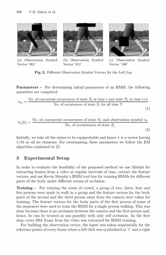
308 C.R. Sahoo et al.
(a) Observation SymbolVector ’001’
(b) Observation SymbolVector ’011’
(c) Observation SymbolVector ’100’
Fig. 2. Different Observation Symbol Vectors for the Left Leg
Parameters - For determining initial parameters of an HMM, the followingquantities are computed:
aij =No. of concurrent occurrences of state Si at time t and state Sj at time t+1
No. of occurrences of state Si for all time T(1)
bj(k) =No. of concurrent occurrences of state Sj and observation symbol vk
No. of occurrences of state Sj
(2)
Initially, we take all the states to be equiprobable and hence π is a vector having1/16 as all its elements. For reestimating these parameters we follow the EMalgorithm explained in [5].
3 Experimental Setup
In order to evaluate the feasibility of the proposed method we use Matlab forextracting frames from a video at regular intervals of time, extract the featurevectors, and use Kevin Murphy’s HMM tool box for training HMMs for differentparts of the body under different scenes of occlusion.
Training - For training the scene of crowd, a group of two, three, four andfive persons were made to walk in a group and the feature vectors for the bodyparts of the second and the third person away from the camera were taken fortraining. The feature vectors for the body parts of the first person of some ofthe sequences were used to train the HMM for a single person walking. This wasdone because there is no occlusion between the camera and the first person and,hence, he can be treated as one possibly with only self occlusion. As the firststep, every fifth frame from the video was extracted for HMM training.
For building the observation vector, the input was taken sequentially for thereference points of every frame where a left click was symbolized as ’1’ and a right

Classification and Quantification of Occlusion Using Hidden Markov Model 309
click was symbolized as ’0’. If a reference point was not visible, an approximatepoint was clicked where the reference point was expected to be present. This wasdone to input the coordinates of the particular body part which influences theextent of body part occluded, and determine the corresponding hidden state fortraining the HMM. The coordinates were taken by clicking at the extremities ofocclusion of the body parts and the states were determined by comparing theextent of occlusion from the coordinates. In certain frames, some portions ofthe body parts were out of the frame, and were assumed to be occluded. Inputfor them could not be provided automatically since they were out of frame andhence the states for these frames were input manually.
Re-estimation of the parameters was done using five iterations of EM algo-rithm. Log likelihood of the model using the parameters after the fifth iterationwas calculated and the parameters along with the log likelihood were saved.
Classification - Observation vector for the given video was built and log likeli-hood (LL) was calculated for all the three classes using the corresponding learntparameters. The video was identified as the class with the closest LL.
Sequence Generation - For sequence generation, parameters of the identifiedclass are taken and Veterbi algorithm as explained in [5] is used to trace backthe hidden states.
4 Experimental Results
We performed experiments on video sequences recorded by our group. The clas-sification results of eighteen sequences comprising of six sequences for each ofthe three classes are represented in the following confusion matrix.
Crowd Opposite Direction Single IndividualCrowd 6 - -
Opposite Direction 2 3 1Single Individual 1 2 3
The rows of the above matrix represent the actual sequences which were usedas input and the columns represent the output of the trained HMM. From theabove matrix it can be seen that the classification for all the six crowd sequencesgiven as input were classified correctly while out of the six sequences of peoplecrossing from opposite direction three were correctly classified and of the sixsequences of single individual again three were correctly classified.
For sequence generation, we take 20 frames from each of the 18 sequences.Out of the 18 sequences, 12 sequences had an accuracy of 75% or more, i.e.,these sequences had at least 15 frames depicting correct state of occlusion.
5 Conclusion
Tracking of people has been the focus of most researchers working with gait asa biometric tool and approximate reconstruction of scene of occlusion with prior

310 C.R. Sahoo et al.
knowledge of articulation. But knowledge of articulation along with the quantityof occlusion and scene of occlusion can help in better approximation.
In this paper we have presented a scheme for classification of the type ofocclusion and quantifying occlusion using hidden Markov model. It takes intoaccount the visible parts of the human body and the states based on occlusionof a band of certain percentage of the body part. The accuracy of the modelcan be increased by refining the states to smaller bands, i.e., 5% or 10% of thebody part. But in that case, the number of states and hence computing cost willincrease. The observation symbol can also be further refined to be six referencepoints instead of three per body part. However, the number of training samplesrequired for that will also go up.
Acknowledgement
This work is partially supported by Alexander von Humboldt Fellowship forExperienced Researchers.
References
1. Apostoloff, N., Fitzgibbon, A.: Learning spatiotemporal t-junctions for occlusiondetection. In: IEEE Computer Society Conference on Computer Vision and PatternRecognition, June 2005, vol. 2, pp. 553–559 (2005)
2. Marchesotti, L., Piva, S., Regazzoni, C.S.: A dynamic model integrating colourand shape information for objects tracking in conditions of occlusion. In: IEEEInternational Conference on Multimedia and Expo, June 2004, vol. 3, pp. 1547–1550 (2004)
3. Mohamed, M.A., Gader, P.: Generalized hidden markov models. ii. application tohandwritten word recognition. IEEE Transactions on Fuzzy Systems 8(1), 82–94(2000)
4. Pan, J., Hu, B.: Robust occlusion handling in object tracking. In: IEEE Conferenceon Computer Vision and Pattern Recognition, June 2007, pp. 1–8 (2007)
5. Rabiner, L.R.: A tutorial on hidden markov models and selected applications inspeech recognition. Proceedings of the IEEE 77(2), 257–286 (1989)
6. Veeravalli, A.G., Pan, W.D., Adhami, R., Cox, P.G.: A tutorial on using hiddenmarkov models for phoneme recognition. In: Proceedings of the Thirty-SeventhSoutheastern Symposium on System Theory, March 2005, pp. 154–157 (2005)
7. Velipasalar, S., Wolf, W.: Multiple object tracking and occlusion handling by infor-mation exchange between uncalibrated cameras. In: IEEE International Conferenceon Image Processing, September 2005, vol. 2, pp. II–418–II–421 (2005)
8. Wang, L., Hu, W., Tan, T.: Recent developments in human motion analysis. Pat-tern Recognition 36(3), 585–601 (2003)
9. Wang, Y., Liu, Z., Zhou, L.: Learning hierarchical non-parametric hidden markovmodel of human motion. In: Proceedings of International Conference on MachineLearning and Cybernetics, August 2005, vol. 6, pp. 3315–3320 (2005)
10. Yilmaz, A., Li, X., Shah, M.: Contour-based object tracking with occlusion han-dling in video acquired using mobile cameras. IEEE Transactions on Pattern Anal-ysis and Machine Intelligence 26(11), 1531–1536 (2004)

IC-Topological Spaces and Applications in Soft
Computing
Subrata Bhowmik
Department of Mathematics, Tripura UniversitySuryamaninagar, Tripura, India-799130subrata bhowmik [email protected]
Abstract. The objective of this paper is to generalize the concept oftopological space so that concepts of approximation spaces like Roughset, Pre-topological space, Approximation spaces generated by arbitraryrelation etc. including topological space can be study by a single space.Here we considered a non-empty set X with two unary operators i and con the power set ℘(X) called respectively the interior and closure opera-tors with some conditions on the operators. We will call the order triplet(X, i, c) an Interior-Closure Topological space or Simply IC-Topologicalspace. In this paper we will discuss some applications of such spaces inreal life problems.
Keywords: Topological Spaces, Incomplete information system.
1 IC-Topological Spaces
In the theory of different types of ”Approximation spaces” like Rough set ap-proximation space, Pre-topological space, Approximation by covering, Approxi-mation spaces generated by a relation etc., the interior/lower approximation andclosure/upper approximation of subsets may not be the interior and closure ofthe subsets with respect to a topology on the set. In this paper we will generalizethe concept of topological space so that all these concepts can unified in a singlespace or its weaker space. This type of newly defined space can be useful inthe study of ”Approximation spaces” and also a useful tool in the the solutionof real life problems like - diagnosis, data compression etc. by establishing softcomputing techniques.
Definition 1. Let X be a non-empty set, we consider two unary operators i andc on ℘(X), i.e. we consider two operators i : ℘(X) → ℘(X) and c : ℘(X) → ℘(X)satisfying the following conditions:
1. For any A⊆X, i(A)⊆c(A) or simply i⊆c.2. i2 = ii = i and c2 = cc = c3. i and c are monotone increasing, i.e. if A⊆B⊆X then i(A)⊆i(B) and
c(A)⊆c(B)4. c(∅)=∅ , i(X)=X
S.O. Kuznetsov et al. (Eds.): PReMI 2011, LNCS 6744, pp. 311–317, 2011.c© Springer-Verlag Berlin Heidelberg 2011

312 S. Bhowmik
The unary operators i and c are respectively called a interior operator and aclosure operator on X and the order triplet (X, i, c) is called a interior-closuretopological space or simply IC-topological space.
For any A⊆X we will say i(A) is the lower approximation of A and c(A) isthe upper approximation of A in the IC-topological space (X, i, c).
If we omit the condition (1), then the order triplet (X, i, c) is called quasi-IC-topological space or qIC-topological space; if we omit the condition (2) only, thenthe order triplet (X, i, c) is called pseudo IC-topological space or pIC-topologicalspace and if we omit both the conditions (1) and (2), then the order triplet (X,i, c) is called quasi-pseudo-IC-topological space or qpIC-topological space,
For a IC-topological space (or qIC or pIC-topological space) (X, i, c) a subsetU⊆X is called an open set if i(U)=U and a subset F⊆X is called a closed set ifc(F)=F. It is easy to see that the whole set X is an open set and the empty set∅ is a closed set.
Example 2. (i) Any topological approximation space (℘(X), O(X), C(X), l, u)induced from a topological space (X, B) (see Cattaneo[1]), (X, l, u) is an IC-Topological space. We can also in similar way generate IC-topological spacetaking a supra topological space in the above approximation space.
(ii) If int and cl are interior and closure operator on a a non-empty set X (seeZhu [10]) then (X, int, cl) ia an IC-topological space.
(iii) Let R be relation on a non-empty set X, for each x∈X we defineRx=y∈X:xRy. We define unary operations i and c on the power set ℘(X) as: forany subset A of X we define i(A)=x∈X:Rx ⊆A and c(A)=x∈X:Rx∩A= ∅.It is very easy to see that (X, i, c) is a qpIC topological space.
(iv) For any rough set approximation space (X, R) generated by an equivalencerelation R on X (see Pawlak[6]), if − and − be the lower and upper approximationoperators respectively, then (X, −, −) is an IC-topological space.
(v) If (℘(X), ∩, ∪, ∼, L, H) is a rough set algebra (see Yao[9]), then (X, L,H) is a qpIC-topological space.
(vi) For a pre-topological space (X, ε, κ) (see Pagliani and Chakraborty[5]),if I and C are corresponding κ-interior and ε-closure operator respectively then(X, I, C) is a IC-topological space.
Some properties of the IC-topological spaces are listed below, the proofs areeasy forward, so proofs are omitted
Theorem 3. For a IC-topological space (X, i, c), for any A, B⊆X,i(A∩B)⊆i(A)∩i(B) and c(A)∪c(B)⊆c(A∪B)
Theorem 4. For a IC-topological space (X, i, c), for A∈X, i(A) contains everyopen set contained in A and c(A) is contained in every closed set containing Aor in other word ∪U: U∈ OO(X) and U⊆A ⊆i(A) and c(A)⊆ ∩F: F∈ C(X)and A⊆F.

IC-Topological Spaces and Applications in Soft Computing 313
Theorem 5. For a IC-topological space (X, i, c) for any A⊆X the conditionsi(X - A)=X - c(A) and c(X - A)=X - i(A) are equivalent.
Definition 6. A IC-topological space (X, i, c) is said to be
(i) proper if for any A⊆X, i(A)⊆A⊆c(A),(ii) with duality if for any A⊆X, i(X - A) = X - c(A).
Example 7. The IC-topological space generated by a rough set approximation isa proper IC-topological space with duality.
Theorem 8. For a IC-topological space (X, i, c) with duality,
(i) for any A⊆X the conditions (i) i(A)⊆A and (ii) A⊆c(A) are equivalent.(ii) U⊆X is open iff X - U is closed.
2 Application in Soft Computing When the Informationfrom the Data Is Incomplete
IC-topological spaces can be use to apply in such problem like prediction, datacompression etc which will be discussed in this section. Here the problems areassociated with the decision with incomplete information. Before going to applyIC-topological spaces in these type of problems, let us first know the definition ofincomplete information system. Following Shao[7], Cattanio[1], Kryszkiewicz[2]we define an incomplete information as:
Definition 9. An Incomplete information system (IIS) is a structure K=(X, Att,Val, F ) where
(i) X is a non-empty set called the sample space,(ii) Att is a non-empty set called the set of attributes,(iii) Val=Y, N called the set of values of attributes associated with the
members of X (Y=Yes, N=No), and(iv) F= fa : a∈Att is a set of mappings called the attributive decision
functions defined as: for each a∈Att there exists a non-empty subset Xa ⊆Xsuch that fa : Xa → Val.
If Xa=X for each a∈Att the information system K=(X, Att, Val, F ) is said tobe complete(CIS).
Now let us assume that for each a∈Att there exists x∈Xa such that fa(x)=Yand for each x∈X, ∃ a∈Att such that x∈Xa with fa(x)=Y. us define two operatorss : Att → ℘(X) and m : Att → ℘(X) as
s(a)=x∈ : fa(x)=Y, m(a)=x∈ : fa(x)=Y∪(X-Xa)We will say s(a) is the set having attribute ”a” surely and m(a) is the set
having attribute ”a” possibly, but no one outside m(a) has the value of theattribute ”a” ”N”.
Let us define attributes ”1” and ”0” and consider the information systemK=(X, Att/, Val/, F/) where Att/=Att∪0, 1 and Val/=Val∪f0, f1 andX1=X=X0, the attribute of possibly any one of the attribute that f1(x)=Y

314 S. Bhowmik
and f0(x)=N for each a∈X. So s(1)=X=m(1) and s(0)=∅=m(0). We can sayattribute ”1” is characterized as: for each x∈X ”1” is the attribute having atleast any one of the attribute from Att with ”Y” and ”0” is characterized as: foreach x∈X ”0” is the attribute having all the attribute from Att with ”N”.
Again we define two operators i : ℘(X) → ℘(X) and m : ℘(X) → ℘(X) asi(A)=∪s(a): a∈Att/ and s(a)⊆Ac(A)=∩m(a) : a∈Att/ and A⊆m(a)It is easy to see that i(A)⊆A⊆c(A).
Theorem 10. (X, i, c) is a IC-topological space.
Proof. 1. i⊆c follows from the definition of i and c.2. For A⊆X, i(A)⊆A, so ii(A)⊆i(A). Let x∈i(A), so x∈s(a)⊆A, so
x∈s(a)⊆i(A), i.e. x∈ii(A), so ii=i.For A⊆X, A⊆c(A), so c(A)⊆cc(A). Let x∈cc(A), so x∈m(a) for any a∈Att/
with c(A)⊆m(a), now for any a∈Att/ with A⊆m(a) ⇒ c(A)⊆m(a), but x∈m(a),i.e. x∈c(A), so cc=c.
3. i and c both are monotonic according to the definition of i and c.4. s(1)⊆X so i(X)=X, ∅⊆m(0) so c(∅)=∅.
Hence (X, i, c) is a IC-topological space.
We define two operators I : ℘(X) → ℘(X) and C : ℘(X) → ℘(X) as
I(A)=∪s(a): a∈Att and s(a)∩A= ∅C(A)=∪m(a) : a∈Att and m(a)∩A= ∅It is very easy to see that:
Theorem 11. (X, I, C) is a pIC-topological space.
We again define two operators ι : ℘(X) → ℘(X) and ε : ℘(X) → ℘(X) as
ι(A)=∪s(a): a∈Att and s(a)⊆Aε(A)=∪m(a) : a∈Att and m(a)∩A= ∅It is also very easy to see that:
Theorem 12. (X, ι, ε) is a pIC-topological space.
For any IIS we can generate different types of approximation spaces as IC-topological spaces as in Theorem10-12.
2.1 A Model of Decision Making When the Information from theData Is Incomplete
Let S be a set or universes of elements with large numbers of objects and a1, a2,...,an; b1, b2, ...,bm, be n+m attributes. Let us say ak’s are symptom attributesand bj ’s are decision attributes. The information is that all the members of Shaving at least one attribute with value ”Y” and also the information is incom-plete. Now the problem is: we are to decide if we pick up an object of S say ”x”and observing the symptom attributes of ”x” we are to decide which decision

IC-Topological Spaces and Applications in Soft Computing 315
attribute is the concluding decision for ”x”. Another problem is if we select asubset W of S, then which decision attribute is corresponding to W.
For this let us take a subset X of S of suitable size and consider the IISs (X,Att(A), Val, F (A)) and (X, Att(B), Val, F (B)), where
Att(A)=a1, a2, .......,anAtt(B)=b1, b2, .......,bnWe now construct the IC-topological spaces (X, iA, cA)) and (X, iB , cB))
according to Theorem10, qIC-topological spaces (X, IA, CA)) and (X, IB , CB))according to Theorem11, (X, ιA, εA)) and (X, ιB , εB)) according to Theorem12.
2.1.1 Decision ModelFor example let a1, a2, .... ,ak be a set of attributes corresponding to ”x”, nowwe are to decide whether ”x” has the decision attribute bj or not. For this wecan apply the following method:
Let (I) s(a1)∩s(a2)∩ .... ∩s(ak)⊆s(bj) and (II) m(a1)∪m(a2)∪ ....∪m(ak)⊇m(bj), i.e. if some one having the attributes a1, a2, .... , ak surelyis surely with the attribute bj and if some one have the possibility of the deci-sion bj then it have the possible attributes a1, a2, .... , ak, some or all but noneed of more attributes for possibility of bj .
Here we will conclude that ”x” has the decision attribute Bj . If the collectiona1, a2,..... ,ak is a smallest collection to hold the above conditions, we say thatwith the least symptom attributes a1, a2,.... ,ak an element has the decisionattribute bj . We will say a1, a2, ...,ak is a LSDAC (Least Symptom DecisionalAttribute Class) for bj .
2.1.2 Decision ModelLet W be any subset of S and we are to decide which decision attribute shouldbe associate with W. For that we consider the following method:
Let U=W∩X, if 1. iA(U)⊇s(bj) and 2. cA(U)⊆m(bj), i.e. 1. any one having thedecision attribute bj surely then it has at least one or more attributes surely,whose surety is (are) only seen in the class U is and 2. if any one have thepossibility of the common symptom attributes that are possibly common to allthe members in the class U, have the possibility of the decision attribute bj .Here we will decide that bj is a decision attribute corresponding to Y.
If we replace the space (X, iA, cA) by (X, ιA, εA) then the conclusion obtainedcan be treated as stronger conclusion than the above and if replace by (X, IA,CA) then the conclusion can be treated as weaker conclusion than the above.
We can revert the role of symptom attribute and decision attributes in above,we can find the cause of a single symptom attribute in multiple decision at-tributes.
Example 13. Here we are going to see how the above model can be applied in Hos-pital Management. Here the example is only for example not on actual data ormedical fact, this example is only to understand the application of above method.
316 S. Bhowmik
Let in a hospital from some patients we have the following informa-tion(recorder data):
Patient Fever(a1) Headac.(a2) Indg.(a3) Cough(a4) Flue(b1) Stom.Inf.(b2)x1 Y Y Y Y Y Yx2 Y Y N Y Y ?x3 ? N N ? Y Nx4 N N N Y ? Nx5 N Y ? ? N ?
Here the symptom attributes are a1, a2, a3, a4 and decision attributes areb1 and b2. Now,
X=x1, x2, x3, x4, x5s(a1)=x1, x2, m(a1)=x1, x2, x3s(a2)=x1, x2, x5, m(a2)=x1, x2, x5s(a3)=x1, m(a3)=x1, x5s(a4)=x1, x2, x4, m(a4)=Xs(b1)=x1, x2, x3, m(b1)=x1, x2, x3, x4,s(b2)=x1, s(b2)=x1, x2, x5.Obviously s(0)=∅ and m(1)=X.Now the collection a1, a4 is the LSDAC for the decision, since (I) s(a1)∩s(a4)
⊆ s(b1) and (II) m(a1)∪m(a4) ⊇ m(b1).Now we can decide that if a person coming to the hospital with symptoms
”Fever” and ”Cough” then we will make a decision that the patient is with”Flue”. In this case the patient can say that he has the problem of ”Headache”or ”Indigestion” or not. For example if a patient comes with the symptoms a1,a2, a4 then it is easy to see that the corresponding decision is also ”Flue”. Herea1, a4 is a LSDAC for ”Flue(b1)”.
Similarly a1, a3 is a LSDAC for ”Stomach Infection(b2)”.Again Let U=x1, x2 is the portion of a community say ”T” of the region
(T is a specific subset of the population of the region of the hospital). Now,i(U)=s(a1)∪s(a3)=x1, x2 and c(U)=m(a1)∩m(a2)∩m(a4)=x1, x2. We seethat i(U)⊇s(b2) and c(U)⊆m(b2).
Now we can make a decision that the disease b2 is generally confined inthe community ”T” and if a patient come from the community ”T” and if hesuffering from the b2 then we can suspect whether this infection comes from hiscommunity or not and if he is not ill or we can expect the possibility of theinfection b2 due to his community(in case of communicative disease).
2.2 Decision of Change of Set of Attributes
Let S be a population and A=a1, a2,.....,an and B=b1, b2,......,bm be two setof attributers in two different stages, A is initial stage and B is the final stage.The information is all the members of S having at least one attribute from thetwo sets of attributes. Now the problem is: we are to decide whether the initialattributes changed to the final attributes or not. Let X be a sample of suitable

IC-Topological Spaces and Applications in Soft Computing 317
size from the population, but the sample having with incomplete informationregarding the attributes we construct the IC-topological space (X, iA, cB) withthe set of attributes A and (X, iB , cB) with the set of attributes B.
2.2.1 Decision ModelIf (1) U is open in (X, iB, cB) then U is open in (X, iA, cA) and (2) F is closedin (X, iB , cB) then F is closed in (X, iA, cA) holds, i.e. (1) if for any subset Bof B ∃ a subset A of A such that if any element of X has one or more attributesform B surely in final stage ⇔ it must had one or more attributes from A surelyat initial stage and (2) for any subset B of B ∃ a subset A of A such that if anyelement of X has the possibility all the attributes from B finally ⇔ it had thepossibility of all the attributes from A initially.
In this case we will make a decision that the set A of attributes is changed tothe set of attributes B.
2.2.2 Decision ModelWe will say the set of attributes A and B are mutually dependent if U⊆X isopen(closed) in (X, iA, cA) iff U is open(closed) in (X, iB , cB).
Acknowledgements. I am thankful to the referees for their suggestions andvaluable comments to revise the paper.
References
1. Cattaneo, G.: The Lattice Topological Approach to Roughness Theory by Approx-imation Spaces. In: Proceedings-Int. Conf. on Rough Sets, Fuzzy Sets and SoftComputing, November 5-7, 2009, pp. 9–74. Serial Pub., New Delhi (2011)
2. Kryszkiewicz, M.: Rough Set Approach to Incomplete Information Systems. Infor-mation Sciences 112, 39–49 (1998)
3. Mashhour, A.S., Allam, A.A., Mahmoud, F.S., Khedr, F.S.: On Supra TopologicalSpaces. Indian J. Pure and Appl. Math. 4(14), 502–510 (1983)
4. Pagliani, P.: Concrete and Formal Pre-Topological Systems and Their Approxi-mate Operators. In: Proceedings-Int. Conf. on Rough Sets, Fuzzy Sets and SoftComputing, November 5-7, 2009, pp. 119–128. Serial Pub., New Delhi (2011)
5. Pagliani, P., Chakraborty, M.K.: A Geometry of Approximation, Rough Set The-ory: Logic, Algebra and Topology of Conceptual Patterns, pp. 406–477. Springer,Heidelberg (2008)
6. Pawlak, Z.: Rough Sets. International Journal of Information and Computer Sci-ence 11(5), 341–356 (1982)
7. Shao, M.W.: A complete Method to Incomplete Information Systems. In: Yao, J.,Lingras, P., Wu, W.-Z., Szczuka, M.S., Cercone, N.J., Slezak, D. (eds.) RSKT 2007.LNCS (LNAI), vol. 4481, pp. 50–59. Springer, Heidelberg (2007)
8. Willard, S.: General Topology. Addison Wesley Publishing Company, Reading(1970)
9. Yao, Y.: Constructive and Algebraic Method of the theory of Rough Sets. Infor-mation Sciences 109, 21–47 (1998)
10. Zhu, W.: Topological Approaches to Covering Rough Sets. Information Science 177,1499–1508 (2007)

Neuro-Genetic Approach for Detecting Changes
in Multitemporal Remotely Sensed Images
Aditi Mandal1, Susmita Ghosh2, and Ashish Ghosh3
1 Ixia Technologies Pvt. Ltd., Sector V, Kolkata, [email protected]
2 Department of Computer Science and Engineering, Jadavpur University, [email protected]
3 MIU and CSCR, Indian Statistical Institute, Kolkata, [email protected]
Abstract. In the present work the searching capability of Genetic Algo-rithms (GAs) is exploited to evolve suitable Hopfield type neural networkarchitectures for optimum change detection of multitemporal remotelysensed images. Experiments carried out on two remote sensing imagesconfirm the effectiveness of the proposed technique.
Keywords: Change detection, Hopfield type neural network, GeneticAlgorithm, Remote sensing, Multitemporal images.
1 Introduction
In remote sensing applications, change detection is the process of identifyingdifferences in the state of an object or phenomenon by analyzing a pair of im-ages acquired on the same geographical area at different times [1]. Two pre-processed images, radiometrically and geometrically [2] corrected, are comparedpixel by pixel to generate a third image, called the difference image. Once im-age comparison is performed, the change detection process can be carried outby adopting either context-insensitive or context-sensitive procedure. Commonlyused context-insensitive techniques are based on image or histogram threshold-ing which do not take into account the spatial correlation between neighboringpixels in the decision process. To overcome this limitation, a distribution free,context-sensitive and unsupervised change detection procedure based on Hop-field network is suggested in [3].
In the aforementioned neural network based change detection procedure [3],each spatial position (pixel) in the difference image is represented by a neuronin the Hopfield network and it is fully connected to its neighboring neurons.But sometimes full connectivity may result in misclassification of a pixel. It is,therefore, necessary to deal with variable connected networks for improving thequality of the change detection map. In this article the searching capability ofGAs is exploited to evolve Hopfield type optimum neural network architecturesfor context-sensitive unsupervised change detection in multitemporal remotelysensed images.
S.O. Kuznetsov et al. (Eds.): PReMI 2011, LNCS 6744, pp. 318–323, 2011.c© Springer-Verlag Berlin Heidelberg 2011

Neuro-Genetic Approach for Change Detection 319
2 Hopfield’s Model of Neural Networks
A Hopfield neural network consists of a set of neurons where output of eachneuron is fed back to each of the other neurons in the network. There is noself feedback loop, and the synaptic weights are symmetric. Depending on theoutput values a neuron can take, there are two types of Hopfield models: discreteand continuous.
2.1 Discrete Model
In the discrete model, neurons are bipolar i.e., the output Vi of neuron i is either+1 or −1. Hopfield defined the energy function of the network [4] as
E = −z∑
i=1
z∑
j=1,i=j
WijViVj −z∑
i=1
IiVj +z∑
i=1
θiVi , (1)
where the weight Wij represents the synaptic interconnection strength from neu-ron j to neuron i, and z is the total number of neurons in the network; θi is thepredefined threshold and Ii is the initial input bias applied externally to theneuron i. The change of energy ΔE due to a change of output state of a neuroni by ΔV is
ΔE = −⎡
⎣z∑
j=1,i=j
WijVj + Ii − θi
⎤
⎦ΔVi = − [Ui − θi] ΔVi. (2)
Any change in Vi makes ΔE negative. At each iteration, the energy valuedecreases and the network reaches a stable state when its energy value reachesthe minimum [4].
2.2 Continuous Model
In this model, the output of a neuron is continuous and Vi lies in the range[−1, +1]. The energy function E of the continuous model is given by
E = −z∑
i=1
z∑
j=1,i=j
WijViVj −z∑
i=1
IiVj +z∑
i=1
1Ri
∫ Vi
0
g−1(Vi)dv. (3)
The function E is a Liapunov function, and Ri is the total input impedanceof the amplifier realizing a neuron i. The last term in (3) is the energy loss term,which becomes zero at the high gain region. Therefore, the only stable pointsof the very high-gain continuous deterministic Hopfield model correspond to thestable points of the discrete stochastic Hopfield model [4].

320 A. Mandal, S. Ghosh, and A. Ghosh
3 Change Detection Based on Modified Hopfield NeuralNetwork Architecture
For change detection of two coregistered and radiometrically corrected multi-spectral images X1 and X2 of size p× q, acquired over the same area at differenttimes T1 and T2, at first the difference image D = lmn, 1 ≤ m ≤ p, 1 ≤ n ≤ qis obtained by applying the CVA technique [1,2], where lmn is the gray valueof the spatial position (m, n). A neuron is assigned to each (m, n) ∈ D asintroduced in [5]. The spatial correlation between neighboring pixels is mod-eled by defining the neighborhood systems N of order d, for a given position(m, n) as Nd
mn = (m, n) + (u, v); (u, v) ∈ Nd. The connection strength betweenthe (m, n)th and (u, v)th neurons Wmn,uv = 1 if (u, v) ∈ Nd
mn; otherwise,Wmn,uv = 0. Each neuron in the network is initialized by external input biasImn which is computed considering the optimal initialization threshold t0 andautomatically derived initialization threshold t1 [3]. The energy function of thenetwork as defined in [5] is as follows
E = −p∑
m=1
q∑
n=1
∑
(u,v)εNdmn
Wmn,uvVmnVuv −p∑
m=1
q∑
n=1
ImnVmn. (4)
In terms of images, the first part of (4) can be seen as the impact of the grayvalues of the neighboring pixels, whereas the second part can be attributed to thegray value of the pixel under consideration [5]. The minimization of (4) resultsin a stable state of the network in which changed pixels (with output +1) areseparated from unchanged ones (with output -1).
4 Architecture Evolution Using GAs for ChangeDetection
The connectivity of a neuron allows the neighborhood information to be used fordeciding the class of the corresponding pixel as changed or unchanged. In case,some of the neighbors are not completely corrected (geometrically or radiomet-rically) in the preprocessing step or the pixel is in boundary region, then fullconnectivity (which considers maximum neighborhood information) may resultin misclassification of the said pixel. It is, therefore, necessary to adopt variableconnected networks for improving the performance of change detection. This willalso enable us to have less connectivity (i.e., less expensive network) as comparedto the fully connected one, besides the improved performance.
Here, each chromosome of a GA [6] represents a network architecture as itis viewed in [7]. For a p × q image, each pixel (neuron) being connected to atmost k of its neighbors, the length of the chromosome is p × q × k. If a neuronis connected to any of its neighbors, the corresponding bit of the chromosome isset to 1, else 0. Each network is allowed to run for change detection as describedin the previous section. The energy value obtained at the converged state ofa network is taken as the index of fitness of the corresponding chromosome

Neuro-Genetic Approach for Change Detection 321
(minimum energy corresponds to maximum fitness) for its selection for the nextgeneration. The best chromosome of the final population represents the Hopfieldtype optimum neural network architecture.
5 Results and Analysis
To assess the effectiveness of the proposed approach, we consider remote sensingdata sets corresponding to geographical area of Mexico which is made up of twomultispectral images acquired by the sensor of the Landsat-7 satellite in April2000 and May 2002 (Figs. 1(a) and 1(b), respectively). Between the two afore-mentioned acquisition dates, a fire destroyed a large portion of the vegetationin the considered region. The corresponding difference image and the referencemap are shown in Figs. 1(c) and 1(d), respectively.
Fig. 1. Images of Mexico area. (a) Band 4 of the Landsat ETM+ image acquiredin April 2000, (b) band 4 of the Landsat ETM+ image acquired in May 2002, (c)corresponding difference image generated by CVA technique, and (d) reference map ofchanged area.
After analyzing the histogram of the difference image (DI) generated by CVAtechnique, we observe that the highest peak is in the region of lower gray value. Ifwe consider the properties of the DI, a reasonable assumption can be as follows:a pixel having lower gray value exhibits a high probability of being in unchangedclass, whereas a pixel with higher gray value has a high probability of being inchanged class. This implies that most of the pixels and their neighbors in thelower gray value region belong to the same area i.e., unchanged area. Hence,for this region maximum neighborhood information can be used for deciding apixel’s class. On the contrary, as nature of the neighbors of rest of the pixels isunknown, use of maximum neighborhood information may lead to their misclas-sification. So we initialize the population of GA in such a way that if a pixel haslower gray value then the corresponding bits in the chromosome will be 1 withthe probability 0.9; otherwise, it will be filled up with 0s and 1s with equal prob-ability. The population size is kept fixed to 50. The generational replacementtechnique and elitist model are adopted here along with linear normalizationselection [6]. Multipoint crossover is implemented where number of cross-sitesis set to 1000 and crossover probability, pc, is set to 0.9. It is expected that in

322 A. Mandal, S. Ghosh, and A. Ghosh
the final architecture we have more 1s than 0s because most of the pixels willbe connected with more than half of their neighbors to use the contextual in-formation. So we carry out the experiment with two different sets of mutationprobabilities pm and pb to preserve 1s more than preserving 0s. We mutate thebit 0 with the probability pm only, whereas bit 1 is mutated with probabilitypm × pb. For second order connectivity, we have taken pm=0.01, pb=0.01. Themutation probability, pm, is decreased to 0.001 in case of the first order connec-tivity as the the length of the chromosome is much less in the first order thanin the second order. The network attains stable state around 350th and 200th
generations for the first and the second order connectivity, respectively.In order to establish the effectiveness of the proposed technique, a comparison
is carried out between the change detection results produced by the proposedGA based method and those using the Hopfield-Type neural networks (HTNN)[3]. Results obtained using both the methods are put in Table 1. It shows thatthe proposed model always produces less overall error (and a network with lessnumber of connections) as compared to the HTNN counterpart. Also, the secondorder connectivity is found to be more effective than the first order.
Table 1. Change detection results obtained by the HTNN and the proposed technique
Figs. 2(a) and 2(b) depict the change detection maps produced by the HTNNand the proposed technique, respectively for the first-order continuous modelwith t1= 31. Figs. 2(c) and 2(d), respectively, show the change detection mapsobtained using the HTNN and the proposed technique for the second orderdiscrete model with t1= 27. A visual comparison points out that the proposedapproach, due to a proper exploitation of the contextual information, generatesa more smooth change detection map compared to the fully connected one.
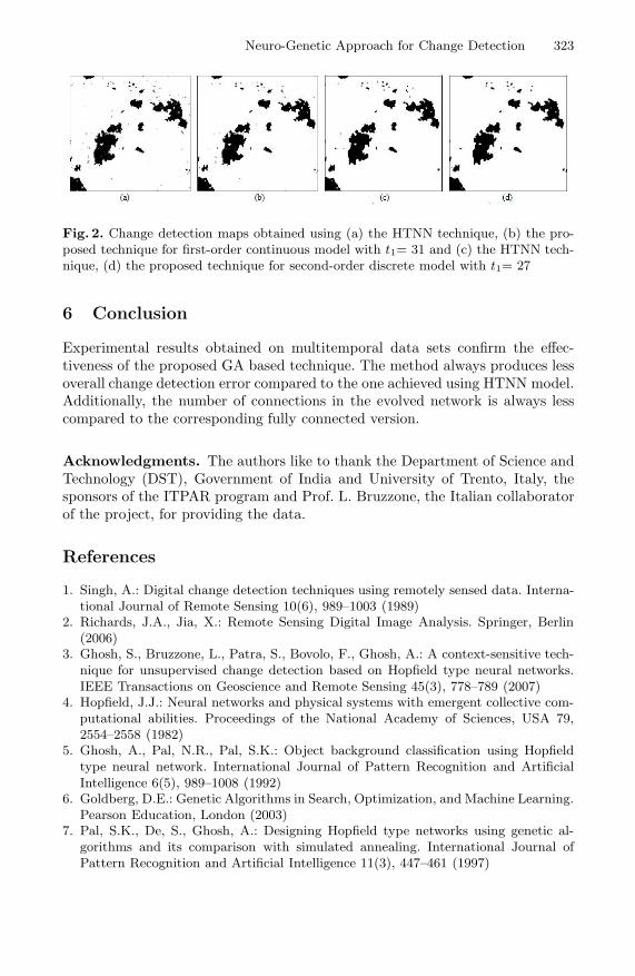
Neuro-Genetic Approach for Change Detection 323
Fig. 2. Change detection maps obtained using (a) the HTNN technique, (b) the pro-posed technique for first-order continuous model with t1= 31 and (c) the HTNN tech-nique, (d) the proposed technique for second-order discrete model with t1= 27
6 Conclusion
Experimental results obtained on multitemporal data sets confirm the effec-tiveness of the proposed GA based technique. The method always produces lessoverall change detection error compared to the one achieved using HTNN model.Additionally, the number of connections in the evolved network is always lesscompared to the corresponding fully connected version.
Acknowledgments. The authors like to thank the Department of Science andTechnology (DST), Government of India and University of Trento, Italy, thesponsors of the ITPAR program and Prof. L. Bruzzone, the Italian collaboratorof the project, for providing the data.
References
1. Singh, A.: Digital change detection techniques using remotely sensed data. Interna-tional Journal of Remote Sensing 10(6), 989–1003 (1989)
2. Richards, J.A., Jia, X.: Remote Sensing Digital Image Analysis. Springer, Berlin(2006)
3. Ghosh, S., Bruzzone, L., Patra, S., Bovolo, F., Ghosh, A.: A context-sensitive tech-nique for unsupervised change detection based on Hopfield type neural networks.IEEE Transactions on Geoscience and Remote Sensing 45(3), 778–789 (2007)
4. Hopfield, J.J.: Neural networks and physical systems with emergent collective com-putational abilities. Proceedings of the National Academy of Sciences, USA 79,2554–2558 (1982)
5. Ghosh, A., Pal, N.R., Pal, S.K.: Object background classification using Hopfieldtype neural network. International Journal of Pattern Recognition and ArtificialIntelligence 6(5), 989–1008 (1992)
6. Goldberg, D.E.: Genetic Algorithms in Search, Optimization, and Machine Learning.Pearson Education, London (2003)
7. Pal, S.K., De, S., Ghosh, A.: Designing Hopfield type networks using genetic al-gorithms and its comparison with simulated annealing. International Journal ofPattern Recognition and Artificial Intelligence 11(3), 447–461 (1997)

S.O. Kuznetsov et al. (Eds.): PReMI 2011, LNCS 6744, pp. 324–332, 2011. © Springer-Verlag Berlin Heidelberg 2011
Synthesis and Characterization of Gold Nanoparticles – A Fuzzy Mathematical Approach
D. Dutta Majumder1, Sankar Karan2, and A. Goswami3
1 ECSU, Indian Statistical Institute, 203, B.T. Road, Kolkata 700108, India
2 Institute of Radiophysics and Electronics, C.U., 92, APC Road, Kolkata 700006, India 3 Biological Science Division, ISI,203, B T Road, Kolkata 700108, India
[email protected], [email protected], [email protected]
Abstract. This article presents the development of nanoparticles (NPs) with potentially useful size and shape dependent properties that have the advantage of ultra-fine size, high surface area and useful interfacial imperfections. When developing NPs as catalysts, their shape is very important. For a certain volume of material, nanoparticles make the best catalysts when they have a large surface area. It is a challenge to find the shape that has the largest surface area for its volume. The particle shape contours were measured by transmission electron microscope with high resolution. These TEM images are analyzed with image clustering techniques and generalized shape theory that results the computational indicators for shape, degree of atomic compactness and charge arrangement of NPs.
Keywords: Fuzzy C-Means Clustering, Generalized Shape Theory & Metric, Nanomaterial, Nanoimaging, Nano Synthesis.
1 Introduction
Nanometer sized(1x10⁻⁹ to 100x10-9)particles are of today’s interests because of their shape and size-dependent[1] physical properties. The chemical and physical properties of such aggregates, comprising only a few hundred atoms are in a transition region between the bulk and individual atomic or molecular properties. By understanding size and shape related changes in these systems, it is hoped that advanced new materials can be developed together with a raft of new technologies. Nanotechnology[2] may be defined as the development at the atomic, molecular and micro-molecular levels in the length and scale of approximately 1-100 nanometer range, to provide a fundamental understanding of phenomena and materials at the nanoscale and to create and use structures, devices and systems that have novel properties and functions because of their size and shape related properties. NPs with potentially useful size and shape dependent properties have the advantage of ultra fine size, high surface area, useful interfacial defects and so are extensively utilized as key components in electronics and optical

Synthesis and Characterization of Gold Nanoparticles 325
devices, pharmaceutics, paints, coatings, superconductors, semi conductors. In fact the reproducible preparation of shape controlled particles using the popular colloid–chemical approach is difficult. Using in-process measurement techniques and particle image analysis, our research characterizes the synthesis of gold NPs improve compactness and sphericalness. This type of characterization helps the researchers in shape and size-based spectral tuning, biological labeling, toxicity studies and suggest general protocols to address these problems.
Imaging beneath the surface of a sample has always been a challenge to microscopy as they cannot be seen in the traditional sense, but that should not prevent us from visualizing the nanoworld. The main goal of Nanotechnology is to analyze and understand the properties of matter at the atomic and molecular level. Non-destructive, nanoscale characterization techniques[3] are needed to understand both synthetic and biological materials. In this paper we propose a new nanoscale image-based characterization techniques to analyze and synthesis nanoscale images that requires algorithms to perform image analysis under extremely challenging conditions such as low signal-to-noise ratio and low resolution. To achieve this, we developed an imaging tools that are able to enhance images [4], detect objects and features [5] and analyze particle size and shape[6]. Here we present the algorithms, describe their representative methods, and conclude with several promising directions of future investigation. Nano scale photograph processing allows us to understand unique properties of matter at atomic and molecular level spanning a wide range of ap-plications in areas such as nano-bio-medicine, nano-chip manufacturing, material sciences, nano-agri-biotechnologies and environmental toxicology[7-8].
2 Materials and Methods
Thiol, aspartic acid, Citrate protected gold nanoparticles of different size and shape were synthesized in the laboratory. Transmission Electron Microscopy(TEM) and spectroscopy study for Imaging and particle size distribution of Gold NPs were performed to observe the topology of the particles. These images are processed by fuzzy logic based clustering techniques. Mean diameter and compactness are measured automatically through algorithms by counting pixels belonging to every clusters. Surface(S) to Volume(V) ratio was measure considering the NPs are spherical in nature. Packing density is obtained by measuring the imperfections/defects from its segmented TEM images. Results are observed, compared with existing method and chemical measurement and manual counting.
2.1 Nano Scale Image Data Clustering Using Fuzzy C-Means(FCM)
TEM Image data of Gold NPs were (20nm ) classified using fuzzy C-Means clustering [9-11] algorithm to separate the particle from its background, identify the defect and also the molecular arrangement inside the particle and developed an

326 D.D. Majumder, S. Karan, and A. Goswami
iterative optimization procedure for classification. Let X = 1X , 2X , … ,
nX be a set of samples to be clustered into c classes. Here we consider color as a
feature for classification in RGB (red, green, blue) color space. The criterion function used for the clustering process is
1
2
1
( )k
n
k ik x C
J V x v= ∈
= −∑ ∑ (1)
Where vi, is the sample mean or the center of samples of cluster i, and V = v1, ... , vc. To improve the similarity of the samples in each cluster, we can minimize this criterion function so that all samples are more compactly distributed around their cluster centers. Membership values (µ’s) are assigned as per FCM algorithm.
In summary, the c-means clustering procedure consists of the following steps:
• S-1: Determine the number of clusters c. • S-2: Partition the input samples into c clusters based on an approximation. If no
rule of approximation exists, the Samples can be partitioned randomly. • S-3: Compute the Cluster Centers • S-4: Assign each input sample to the class of the closed cluster center. • Repeat steps 3 and 4 until no change in J can be made and the algorithm
converges. For cluster validity[11-12], we consider three types of measures : partition
coefficient, partition entropy and compactness and separation validity function.
2.2 Shape Based Image Registration of Gold NP’s
The perception of shape has been used for pattern recognition, computer vision, shape analysis[13], and image registration. Here we proposed a generalized method of shape analysis and shape based similarity measures, shape distance and shape metric to measured the NPs shape. The shape of an object can be defined as a subset X in R2 if (a) X is closed and bounded, (b) Interior of X is non-empty and connected and (c) Closure property holds on interior of X. This representation of shape remains invariant with respect to translation, rotation and scaling. Moreover another object Y in R2 is of same shape to object X ∈ R2 if it preserves translation, rotation and scaling invariance. In term of set these three transformations can be represented as
Translation : Y = (x + a),(y + b): x, y∈ X (2)
Rotation : Y = P1(α).P2(β)X where P1 & P2 are rotation around x and y axes. (3)
Scaling : Y = (kx, ky): x, y ∈ X (4)
Distance d1 between shape X and Y in F is defined as follows: d1(X,Y)=m2[(X-Y)∪(Y-X)] (5)

Synthesis and Characterization of Gold Nanoparticles 327
where m2 is Lebesgue measure in R2 and d1 satisfies following rules: (i) d1(X,Y) ≥ 0, (ii) d1(X,Y) = 0 if and only if X = Y (iii) d1(X,Y) = d1(Y,X) and (iv) d1(X,Y) + d1(Y,Z) ≥ d1(X,Z. We consider, two nano particles are of same shape if and only if one of the image is translation, Scaling and rotation of other.
• Shape extraction and similarity measure
To extract the feature of the boundary of the Region of Interest(ROI) it is helpful to represent the closed contour with a set of direction. The direction code may be taken among “n” selected points on the contour, which has same distance between any two consecutive points. The direction d makes an angle 45° with direction i, where real number d ∈1 to 8 and i = (1,2,..8). Let dm= (dij), j= 1 to n where m = A, B are the contour starting from each reference point A and B and are denoted by dA and dB respectively. If d2 is a rotation of d1 then d2= d1 + γ for any real number γ. For all j we can write d2= d1 + γ ∀ j and the distance function D, in terms of the direction code between the contour of interest and the model is defined as:
n D(d1d2) = ∑ min((d1jd2j),8 - (d1jd2j)) (6) J=1
The normalized value of D is D/n and the shape similarity measure between the two shapes is given by μ = 1-D/n, smaller value of D indicates higher degree of similarity [13].
Fig. 1. Chain code representation
3 Experimental Procedure and Results
• Synthesis of thiol protected gold nanoparticle
Aqueous solution of HAuCl4 is mixed with solution of ToABr in toluene. Vigorous
stirring causes transfer of HAuCl4 into the organic layer. Dodecanethiol is added to
the organic phase followed by addition of aqueous solution of NaBH4 is slowly added with vigorous stirring. Aqueous solution of sodium borohydride is slowly added with vigorous stirring. A deep brown coloured solution appears at the interface. Excess ethanol is added to the separated brown coloured solution and kept overnight which

328 D.D. Majumder, S. Karan, and A. Goswami
causes precipitation of GNP. The ethanolic solution is filtered with nylon filter and the precipitate is re-dispersed in toluene
• Synthesis of aspartic acid protected gold nanoparticle
90 ml of 10-4M aqueous solution of chloroauric acid is prepared. The solution is heated up to boiling condition. 10 ml of 10-2M aspartic acid solution is added to the boiling solution. Aspartic acid acts as the reducing agent. The reduction process is continued under constant stirring. Heating is stopped. The reduction of the metal ions is evident with appearance of red color.
• Synthesis of Citrate capped gold nanoparticle
50 ml of 1mM aqueous solution of chloroauric acid is prepared. The solution is heated up to boiling under reflux condition. 5 ml of 1% tri sodium citrate dihydrate solution is added to the boiling solution. Sodium citrate here reduces the gold chloride. Stirring was continued until the color of the solution gradually changed from faint yellowish to clear to grey to purple to deep purple, and finally wine-red. Negatively charged citrate ions were absorbed onto the GNPs, introducing the surface charge that repels the particles and prevents them from aggregation.
Table 1. TEM imaging, absorbance study, shape tracing and size distribution of Gold nanoparticles
Fig. 2. TEM image of thiol capped gold
nanoparticle (3-5nm)
Fig. 3. Surface Plasmon Resonant (SPR) Peak of
thiol capped gold nanoparticle
Fig. 4. TEM image of aspartic acid coated gold
nanoparticle
Fig. 5. SPR spectra of aspartic acid capped gold nanoparticle
Fig. 6. TEM image of citrate capped gold
nanoparticle
Fig. 7. SPR spectra of citrate capped gold
nanoparticle
Fig. 8. Trace of Gold nanoparticles 20nm for its
shape measurement in TEM image
Fig. 9. Size distribution of Gold nanoparticles 20 nm with an
average size of 28.33nm.

Synthesis and Characterization of Gold Nanoparticles 329
Table 2. Image Segmentation using Fuzzy C-Means
Fig. 10. Pixel value with Membership after clustering into 3 classes, with cluster centre V1,V2,V3
Fig. 11. Original TEM Image of Gold nanoparticles 20nm
Fig. 12. Segmented TEM Image of Gold nanoparticles 20 nm in 3 classes
4 Conclusion
A novel and simple method for measurement of the size, shape and other spectral response of gold NPs. These values may be used as the input of Artificial Neural Networks(ANN) to characterized the synthesis process of gold NPs as proposed in fig.15. The ANN offers a successful tool for NPs preparation analysis and modeling. Chemical routes for the Polymer based nanocomposits preparation offer the advantage of (a) a cluster or atomic level control, and (b) an efficient scale up for processing and production. Here the size and shape of the nanoparticles are measured using fuzzy based clustering and shape analysis and gives better results than automatic threshold generator. The high degree of particle size and shape measurement in the nm range suggest a successful application of this method to conclude the signature of quantum size effects occurring in the gold nano particles, realization of color filters, UV absorbers with particularly interesting performances. The flexibility offered by the choice of different polymeric agents as a future element of interest towards future advances in nano-optical and nano-bio applications.

330 D.D. Majumder, S. Karan, and A. Goswami
Table 3. Packing Density and S/V Measurement of Gold NP’s (2nm)
Fig. 13. Comparison of S/V of Gold NPs of 2nm range with
its normal value.
Fig. 14. Surface plot of Packing Density. X- Defect, Y-molecule occupied, Z- Packing Density
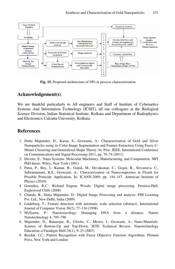
Synthesis and Characterization of Gold Nanoparticles 331
Fig. 15. Proposed architecture of NPs in process characterization
Acknowledgement(s)
We are thankful particularly to All engineers and Staff of Institute of Cybernetics Systems And Information Technology (ICSIT), all our colleagues at the Biological Science Division, Indian Statistical Institute, Kolkata and Department of Radiophysics and Electronics, Calcutta University, Kolkata.
References
1. Dutta Majumder, D., Karan, S., Goswami, A.: Characterization of Gold and Silver Nanoparticles using its Color Image Segmentation and Feature Extraction Using Fuzzy C-Means Clustering and Generalized Shape Theory. In: Proc. IEEE, International Conference on Communications and Signal Processing-2011, pp. 70–74 (2011)
2. Drexler, E.: Nano Systems: Molecular Machinery, Manufacturing, and Computation. MIT PhD thesis. Wiley, New York (1991)
3. Patra, P., Roy, I., Kumar, R., Gopal, M., Devakumar, C., Gogoi, R., Srivastava, C., Subramanium, B.S., Goswami, A.: Characterization of Nanocomposites in Flyash for Possible Pesticide Application. In: ICANN-2009, pp. 144–147. American Institute of Physics (2010)
4. González, R.C.: Richard Eugene Woods: Digital image processing. Prentice-Hall, Englewood Cliffs (2008)
5. Chanda, B., Dutta Majumder, D.: Digital Image Processing and analysis. PHI Learning Pvt. Ltd., New Delhi, India (2009)
6. Lindeberg, T.: Feature detection with automatic scale selection (abstract). International Journal of Computer Vision 30(2), 77–116 (1998)
7. Myllynen, P.: Nanotoxicology: Damaging DNA from a distance. Nature Nanotechnology 4, 795–796
8. Majumder, D., Banaerjee, R., Ulrichs, C., Mewis, I., Goswami, A.: Nano-Materials: Science of Bottom-Up and Top-Down, IETE Technical Review. Nanotechnology Education–a Paradigm Shift 24(1), 9–23 (2007)
9. Bezdek, J.C.: Pattern Recognition with Fuzzy Objective Function Algorithms. Plenum Press, New York and London

332 D.D. Majumder, S. Karan, and A. Goswami
10. Bezdek, J.C., Ehrlich, R., Full, W.: FCM: The fuzzy c-means clustering algorithm. Computers & Geosciences 10(2-3), 191–203 (1984)
11. Bezdek, J.C., Hathaway, R.J., Sabin, M.J., Tucker, W.T.: Convergence theory for fuzzy C-means: counter examples and repairs. IEEE Trans. Syst. Man Cybern., 17873–17877 (1987)
12. Hathaway, R.J., Hu, Y.: Density-weighted fuzzy c-means clustering. IEEE Transactions on Fuzzy Systems 17(1), 243–252 (2009)
13. Parui, S., Sarma, E., Majumder, D.: How to discriminate shape using shape vector. Pattern Recognition Lett. 4, 201–204 (1986)
14. Dutta Majumder, D.: A Study on a Mathematical Theory of Shapes In Relation To Pattern Recognition And Computer Vision. India Journal of Theoretical Physics 43(4), 19–30 (1995)
A Rough Set Based Decision Tree Algorithm
and Its Application in Intrusion Detection
Lin Zhou and Feng Jiang
College of Information Science and Technology, Qingdao University of Science andTechnology, Qingdao 266061, P.R. China
Abstract. In this paper, we propose a novel rough set based algorithmto induce decision trees. To improve the computation efficiency of ouralgorithm, the rough set based attribute reduction technology is usedto filter out the irrelevant attributes from the original set of attributes.And the notions of the significance of attribute and the uniformity ofattribute in rough sets are adopted as the heuristic information for theselection of splitting attributes. Moreover, we apply the proposed algo-rithm to intrusion detection. The experimental results demonstrate thatour algorithm can provide competitive solutions efficiently.
Keywords: Rough sets, decision trees, significance of attribute, unifor-mity of attribute, intrusion detection.
1 Introduction
Decision tree algorithms are used extensively in data mining [1-2]. Since most ofthe current algorithms use all attributes to construct decision trees, and do notconcern the relevancy among attributes [1-2]. This may lead to extra overhead interms of memory and computational efforts [5-6]. To solve that problem, roughset-based decision tree algorithms have been proposed within last few years [3-6].
Intrusion detection systems (IDS) have become an essential component ofcomputer security. The concept of IDS was first introduced by Anderson in 1980[7]. Due to the large volumes of security audit data as well as complex anddynamic properties of intrusion behaviors, to optimize the performance of IDS,many artificial intelligence techniques have been utilized, where decision treetechnology plays an important role in IDS [8].
In this paper, we propose a novel rough set based decision tree algorithmRSDT and apply it to IDS. In our algorithm, the rough set based attributereduction technology is used to filter out redundant information, which is crucialto IDS. Moreover, we introduce a new concept called the uniformity for eachattribute in a given decision table. And we use the significance of attributeand the uniformity of attribute as the heuristic information for the selection ofsplitting attributes. Numerical experiments show that our algorithm is efficientfor intrusion detection.
S.O. Kuznetsov et al. (Eds.): PReMI 2011, LNCS 6744, pp. 333–338, 2011.c© Springer-Verlag Berlin Heidelberg 2011
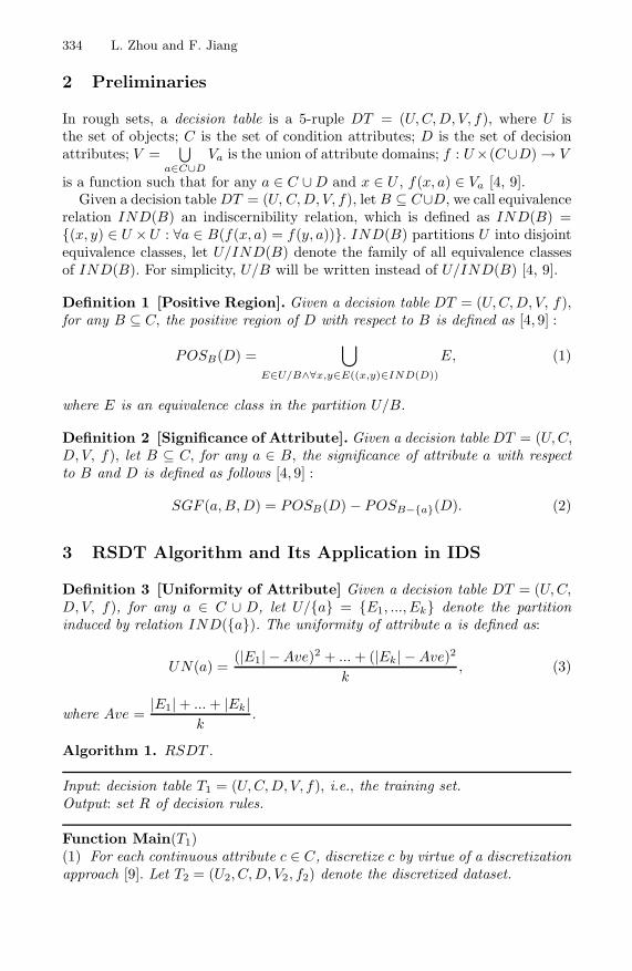
334 L. Zhou and F. Jiang
2 Preliminaries
In rough sets, a decision table is a 5-ruple DT = (U, C, D, V, f), where U isthe set of objects; C is the set of condition attributes; D is the set of decisionattributes; V =
⋃a∈C∪D
Va is the union of attribute domains; f : U×(C∪D) → V
is a function such that for any a ∈ C ∪ D and x ∈ U , f(x, a) ∈ Va [4, 9].Given a decision table DT = (U, C, D, V, f), let B ⊆ C∪D, we call equivalence
relation IND(B) an indiscernibility relation, which is defined as IND(B) =(x, y) ∈ U ×U : ∀a ∈ B(f(x, a) = f(y, a)). IND(B) partitions U into disjointequivalence classes, let U/IND(B) denote the family of all equivalence classesof IND(B). For simplicity, U/B will be written instead of U/IND(B) [4, 9].
Definition 1 [Positive Region]. Given a decision table DT = (U, C, D, V, f ),for any B ⊆ C, the positive region of D with respect to B is defined as [4, 9] :
POSB(D) =⋃
E∈U/B∧∀x,y∈E((x,y)∈IND(D))
E, (1)
where E is an equivalence class in the partition U/B.
Definition 2 [Significance of Attribute]. Given a decision table DT = (U, C,D, V, f ), let B ⊆ C, for any a ∈ B, the significance of attribute a with respectto B and D is defined as follows [4, 9] :
SGF (a, B, D) = POSB(D) − POSB−a(D). (2)
3 RSDT Algorithm and Its Application in IDS
Definition 3 [Uniformity of Attribute] Given a decision table DT = (U, C,D, V, f), for any a ∈ C ∪ D, let U/a = E1, ..., Ek denote the partitioninduced by relation IND(a). The uniformity of attribute a is defined as:
UN(a) =(|E1| − Ave)2 + ... + (|Ek| − Ave)2
k, (3)
where Ave =|E1| + ... + |Ek|
k.
Algorithm 1. RSDT .
Input: decision table T1 = (U, C, D, V, f), i.e., the training set.Output: set R of decision rules.
Function Main(T1)(1) For each continuous attribute c ∈ C, discretize c by virtue of a discretizationapproach [9]. Let T2 = (U2, C, D, V2, f2) denote the discretized dataset.

A Rough Set Based Decision Tree Algorithm and Its Application 335
(2) Compute the reduct Red of C with respect to D in T2, using a rough setbased attribute reduction approach [9-11, 16].(3) Reduce T2 based on the reduct Red. Let T3 = (U3, Red, D, V3, f3) denote thereduced dataset.(4) Decision Tree(T3). //Call a function defined below to induce a decision tree.(5) Generate a set R of rules by traversing all the paths from the root to the leafnode in the decision tree.(6) Return R.
Function Decision Tree(Tcurrent) // Tcurrent = (U ′, C ′, D, V ′, f ′) is thedecision table that is currently in use.
(1) For each attribute a ∈ C′, calculate the significance SGF (a, C′, D) of a withrespect to C′ and D in Tcurrent.(2) Select t from C′ with the largest significance as the splitting attribute.(3) If there exist more than one attributes with the largest significance, then cal-culate the uniformity for each of these attributes in Tcurrent, and select attributet with the largest uniformity (If there still exist more than one attributes withthe largest uniformity, then arbitrarily select one from them).(4) Create a node N, label N with attribute t, and let C′ = C′ − t.(5) For each value vj of attribute t
(5.1) Generate one branch of N, labeled with t = vj ;(5.2) Let Sj = o ∈ U ′ : f ′(o, t) = vj;(5.3) If Sj = ∅, then add one leaf node L labeled with the most common
class in U ′;(5.4) If Sj = ∅, and all objects in Sj belong to the same class d, then add
one leaf node L labeled with the class d;(5.5) If Sj = ∅, C ′ = ∅, and objects in Sj belong to different classes, then
add a leaf node L labeled with the most common class in Sj.(5.6) If Sj = ∅, C ′ = ∅, and objects in Sj belong to different classes, then
obtain a sub-table Tsub = Sj, C′, D, Vsub, fsub of Tcurrent, and call
function Decision Tree (Tsub) to construct a sub-tree.
In algorithm 1, before computing the partition U ′/C ′, we first sort all objectsof U ′ based on the counting sort [11], then we can calculate U ′/C′ in O(m ×n) time, where m = |C′|, n = |U ′|. Hence, we can calculate the significanceSGF (a, C′, D) of a in O(m × n) time. Therefore, in the worst case, the timecomplexity of step (4) in function Main is O(|Red|3 × |U3|). And the overalltime complexity of algorithm 1 is also determined by that of the discretizationapproach and that of the attribute reduction approach in Main [9-11, 16].
4 Experiment
To evaluate the performance of RSDT algorithm, we ran it on KDD-99 dataset[12]. Experiments were conducted on a 2.0GHz Pentium 4 machine with 2GBRAM. We compared algorithm RSDT with algorithms ID3 and C4.5 [1-2]. RSDTwas implemented in Pascal. And ID3 and C4.5 are available in Weka [13].

336 L. Zhou and F. Jiang
Since the full KDD-99 training dataset is too large for our purposes, a concisesubset of KDD-99, known as ‘10%KDD’, will be discussed here. The 10%KDDdataset contains 22 different attack types and normal records. The 22 attacktypes fall into four main categories [12]: PROBE, DoS, U2R and R2L.
Although the 10%KDD dataset is a concise subset of the full KDD-99 trainingdataset, it contains 494021 records [12], which is still very large for our purposes.Here we follow the experimental technique of Chen et al. [14], which does ran-dom sampling without replacement from the 10%KDD dataset to form a smallerdataset called ‘Final Dataset’. The following table gives the numbers of instancesthat are selected for different attack types and normal records.
Table 1. The numbers of instances selected
Attack Number of Number of Ins- Attack Number of Number of Ins-Type Instances tances Selected Type Instances tances Selected
back 2203 220 perl 3 3
buffer overflow 30 30 phf 4 4
ftp write 8 8 pod 264 264
guess passwd 53 53 portsweep 1040 104imap 12 12 rootkit 10 10
ipsweep 1247 125 satan 1589 160
land 21 21 smurf 280790 2808
loadmodule 9 9 spy 2 2
multihop 7 7 teardrop 979 100
neptune 107201 1072 warezclient 1020 102
nmap 231 231 warezmaster 20 20
normal 97278 9730 Total 494021 15095
There are four steps in our experiments:
(I) The first step is to prepare the dataset. As mentioned above, we do randomsampling without replacement from the 10%KDD dataset to obtain a new datasetcalled Final Dataset.
(II) Next is the discretization step. We use two simple discretization algo-rithms: Equal Width Binning (EW) and Equal Frequency Binning (EF), to re-spectively discretize the continuous attributes in Final Dataset [9]. EW and EFalgorithms are also available in Weka [13]. And for both of the two algorithms,the numbers of bins are set to 3. It should be noted that although Final Datasetcontains 34 continuous attributes, we only discretize the following 26 attributes ofthem: (1) Duration; (2) Src bytes; (3) Dst bytes; (4) Hot; (5) Num compromised;(6) Num root; (7) Num file creations; (8) Count; (9) Srv count; (10) Serror rate;(11) Srv serror rate; (12) Rerror rate; (13) Srv rerror rate; (14) Same srv rate;(15) Diff srv rate; (16) Srv diff host rate; (17) Dst host count; (18) Dst hostsrv count; (19) Dst host same srv rate; (20) Dst host diff srv rate; (21)Dst host same src port rate; (22) Dst host srv diff host rate; (23) Dst hostserror rate; (24) Dst host srv serror rate; (25) Dst host rerror rate; (26) Dsthost srv rerror rate.

A Rough Set Based Decision Tree Algorithm and Its Application 337
Moreover, each discretized Final Dataset is randomly divided into a trainingdataset (60% of the data) and a test dataset (40% of the data).
(III) The third step is constructing decision trees on training datasets usingalgorithms RSDT, ID3 and C4.5, respectively. Then different sets of rules canbe generated from these trees. It should be noted that before applying RSDTto each training dataset, we first reduce the dataset by virtue of the attributereduction algorithm proposed by Liu et al. [10].
(IV) The last step is applying the rules generated in (III) to classify the testdataset based on a given classifier. For ID3 and C4.5, the process is also imple-mented in Weka [13]. And for RSDT, we adopt the Standard Voting classifieravailable in Rosetta [15]. The corresponding options are: CLASSIFIER= Stan-dardVoter; FALLBACK= True; FALLBACK.CLASS=DoS.
Tables 2 details the classification results of different decision tree algorithmson the dataset discretized by EW algorithm.
Table 2. The classification results on the dataset discretized by EW
Decision Tree Number of Classification Time Taken toAlgorithm Attributes Accuracy(%) Build Model(s)
RSDT 24 97.88 0.297
ID3 41 97.665 1.06
C4.5 41 97.582 1.63
From Table 2, we can see that for the dataset discretized by EW, RSDTalgorithm perform better than ID3 and C4.5. Our algorithm generates a betterrule learning scheme for IDS than the other two algorithms, since the detectionrate (i.e., classification accuracy) of our algorithm is obviously higher than thoseof other algorithms, while the training time (i.e., time taken to build model) ofour algorithm is much lower than those of other algorithms.
Moreover, the following table details the classification results of different de-cision tree algorithms on the dataset discretized by EF algorithm.
Table 3. The classification results on the dataset discretized by EF
Decision Tree Number of Classification Time Taken toAlgorithm Attributes Used Accuracy(%) Build Model(s)
RSDT 15 99.255 0.079
ID3 41 99.023 0.83
C4.5 41 98.924 0.74
From Table 3, it is easy to see that for the dataset discretized by EF, RSDTalgorithm also has the best performance. Hence, this experiment also demon-strates the effectiveness of our decision tree algorithm for intrusion detection.
5 Conclusion
In this paper, a novel algorithm based on the significance of attribute and theuniformity of attribute in rough set theory was proposed for constructing decision

338 L. Zhou and F. Jiang
trees. Differing from traditional algorithms, our algorithm employed a new kindof heuristic information for the selection of splitting attributes. And the positiveregion based attribute reduction technology was used to execute pre-pruning fordecision trees, thus the attributes which are not correlated with the decisioninformation are deleted and the total nodes of decision trees are limited. Hence,our algorithm is suitable to deal with the mass data in IDS. Experimental re-sults on the KDD-99 dataset showed that our algorithm generated a better rulelearning scheme for IDS than other algorithms.
Acknowledgements
This work is supported by the National Natural Science Foundation of China(grant nos. 60802042, 61035004), and the Natural Science Foundation of Shan-dong Province, China (grant nos. ZR2009GQ013, ZR2010FQ027).
References
1. Quinlan, R.: Induction of decision trees. Machine Learning 1(1), 81–106 (1986)2. Quinlan, R.: C4.5: Programs for Machine Learning. Morgan Kaufmann, San Fran-
cisco (1993)3. Pawlak, Z.: Rough Sets. Int. J. Comput. Informat. Sci. 11(5), 341–356 (1982)4. Pawlak, Z.: Rough Sets: Theoretical Aspects of Reasoning about Data. Kluwer
Academic Publishing, Dordrecht (1991)5. Li, X.P., Dong, M.: An algorithm for constructing decision tree based on variable
precision rough set model. In: Proc. of the 4th Int. Conf. on Natural Computation,pp. 280–283 (2008)
6. Jiang, Y., Li, Z.H., Zhang, Q., Liu, Y.: New method for constructing decision treebased on rough set theory. Computer Appliactions 24(8), 21–23 (2004)
7. Anderson, J.P.: Computer Security Threat Monitoring and Surveillance. James P.Anderson Co., Fort Washington (1980)
8. Li, X.Y., Ye, N.: Decision tree classifiers for computer intrusion detection. Journalof Parallel and Distributed Computing Practices 4(2), 179–190 (2001)
9. Wang, G.Y.: Rough set theory and knowledge acquisition. Xian Jiaotong UniversityPress (2001)
10. Liu, S.H., Sheng, Q.J., Wu, B., Shi, Z.Z.: Research on efficient algorithms for roughset methods. Chinese Journal of Computers 26(5), 525–529 (2003)
11. Xu, Z.Y., Liu, Z.P., Yang, B.R., Song, W.: A Quick Attribute Reduction Algorithmwith Complexity of max(O(|C||U |), O(|C|2|U/C|)). Chinese Journal of Comput-ers 29(3), 391–399 (2006)
12. KDD Cup 99 Dataset (1999),http://kdd.ics.uci.edu/databases/kddcup99/kddcup99.html
13. Witten, I.H., Frank, E.: Data Mining: Practical Machine Learning Tools and Tech-niques with Java Implementations. Morgan Kaufmann, San Francisco (2000)
14. Chen, S.T., Chen, G.L., Guo, W.Z., Liu, Y.H.: Feature Selection of the IntrusionDetection Data Based on Particle Swarm Optimization and Neighborhood Reduc-tion. Journal of Computer Research and Development 47(7), 1261–1267 (2010)
15. Øhrn, A.: Rosetta Technical Reference Manual (1999),http://www.idi.ntnu.no/_aleks/rosetta
16. Banerjee, M., Mitra, S., Banka, H.: Evolutionary-Rough feature selection in geneexpression data. IEEE Transactions on Systems, Man, and Cybernetics, Part C:Applications and Reviews 37, 622–632 (2007)

Information Systems and Rough Set
Approximations: An Algebraic Approach
Md. Aquil Khan1 and Mohua Banerjee2
1 The Institute of Mathematical Sciences,C.I.T Campus, Chennai 600113, India
[email protected] Department of Mathematics and Statistics,
Indian Institute of Technology, Kanpur 208016, [email protected]
Abstract. The article proposes an algebraic formalism of (complete/incomplete) information systems. Besides providing a complete descrip-tion of information systems, the formalism captures the notion of roughset approximations that are induced by information systems.
1 Introduction
Rough set theory proposed by Pawlak involves two key notions: set approxi-mations and information systems. It considers a situation where we only havepartial information about a set U of objects, represented by an equivalence rela-tion R on U . The pair (U, R) is called an approximation space [8] The relation Rinduces lower and upper approximation operators R and R on ℘(U), the powerset of U , as follows. Let R(x) denote y ∈ U : (x, y) ∈ R.
R(X) := x ∈ U : R(x) ⊆ U, and R(X) := x ∈ U : R(x) ∩ X = ∅.A practical realization of Pawlak’s approximation spaces comes from the notionof complete information systems defined as follows.
Definition 1. A complete information system (CIS) S := (U,A,⋃
a∈A Va, f),comprises a non-empty set U of objects, A of attributes, Va of attribute valuesfor each a ∈ A, and f : U ×A → ⋃
a∈A Va such that f(x, a) ∈ Va.
Given a CIS S := (U,A,⋃
a∈A Va, f), and B ⊆ A, we obtain an approximationspace (U, IndS
B), where(x, y) ∈ IndSB if and only if f(x, a) = f(y, a), for all a ∈ B.
IndSB is called the indiscernibility relation induced by B.An algebraic approach to rough set theory was first presented by Iwinski in
1987 [6]. Since then, substantial work has been done on algebraic aspects of thetheory. In one direction, different representations of rough sets have been con-sidered, and endowed with algebraic structures. It is observed that the algebrasinduced from approximation spaces are instances of various known as well as newalgebraic structures, such as quasi-Boolean algebra, double Stone algebra, Nel-son algebra, Lukasiewicz algebra, topological quasi-Boolean algebra. A detailed
S.O. Kuznetsov et al. (Eds.): PReMI 2011, LNCS 6744, pp. 339–344, 2011.c© Springer-Verlag Berlin Heidelberg 2011

340 M.A. Khan and M. Banerjee
survey can be found in [1]. In the other direction of research, approximationoperators are viewed as abstract unary operators, which leads us to a class ofBoolean algebra with operators (BAO). In fact, a CIS S := (U,A,
⋃a∈A Va, f)
determines an algebra (℘(U),∩,∼, ∅, IndSBB⊆A), where ∅ denotes the emptyset, ∼, complementation relative to U , and ∩, intersection. In [4], such an algebrais called a knowledge approximation algebra of type A derived from CIS S. Anabstract algebra for this class of algebras is proposed in [4], and a correspondingrepresentation theorem obtained.We note that the knowledge approximation algebra derived from a CIS S doesnot give a complete description of the CIS. In fact, attribute, attribute-valuepairs, which are the main ingredients of a CIS, do not appear in this descrip-tion. In this article, our aim is to propose an algebraic formalism of CISs whichcaptures this aspect. Moreover, it also captures the notion of approximationsdefined on CISs. In Sect. 2, we shall consider an algebra induced by CISs. Anabstract algebra is then proposed, of which such an induced algebra is an in-stance. Properties of the proposed abstract algebra are explored. Sect. 3 providesthe corresponding representation theorem. Sect. 4 concludes the article.
2 Algebra for Complete Information Systems
Let us fix finite sets A of attributes and V :=⋃
a∈A Va of attribute values.Let D denote the set of all descriptors [9], viz. pairs (a, v), for each a ∈ A,v ∈ Va. Observe that, given a complete information system S := (U,A,V, f ),each descriptor (a, v) determines a nullary operation (constant) cS(a,v) on ℘(U):
cS(a,v) := x ∈ U : f(x, a) = v.Thus we have the following definition. Let Ω be the tuple (A,V).
Definition 2. Let S := (U,A,V, f ) be a complete information system. A com-plete information system algebra (in brief, CIS-algebra) of type Ω generated bythe complete information system S is the structure
S∗ := (℘(U),∩,∼, ∅, IndSBB⊆A, cSγ γ∈D).
Observe that a CIS-algebra generated by a CIS S is actually an extension of theknowledge approximation algebra derived from S with a collection of nullaryoperations.
One can show that a CIS-algebra satisfies the properties listed below.
Proposition 1. 1.⋃
v∈VacS(a,v) = U .
2. cS(a,v) ∩ cS(a,u) = ∅ when v = u.3. IndS
C(X) ⊆ IndSB(X) for C ⊆ B ⊆ A, and X ⊆ U .
4. cS(a,v) ⊆ IndSa(cS(a,v)).
5. cS(b,v) ∩ IndSB∪b(X) ⊆ IndSB(∼ cS(b,v) ∪ X), X ⊆ U .
6. IndS∅ (X) = ∅ implies X = U .

Information Systems and Rough Set Approximations 341
We shall see later that these properties are actually characterizing properties ofCIS-algebras. Thus, we propose the following notion of an abstract CIS-algebra.
Definition 3. An abstract CIS-algebra of type Ω is a tupleA := (U,∧,¬, 0, LBB⊆A, dγγ∈D),
where (U,∧,¬, 0) is a Boolean algebra and LB and dγ are respectively unary andnullary (constant) operations on U satisfying the following:
(C1)∨
v∈Vad(a,v) = 1;
(C2) d(a,v) ∧ d(a,u) = 0 when v = u;(C3) LC(x) ≤ LB(x) for C ⊆ B ⊆ A;(C4) d(a,v) ≤ La(d(a,v));(C5) d(b,v) ∧ LB∪b(x) ≤ LB(¬d(b,v) ∨ x);(C6) L∅(x) = 0 implies x = 1.
As a consequence of Proposition 1, the CIS-algebra S∗ generated by a CIS S isan abstract CIS-algebra.
Let UB be the dual of the operator LB, that is, UB(x) := ¬LB(¬x). Thefollowing proposition presents a few properties of abstract CIS-algebras.
Proposition 2. 1. UB(0) = LB(0) = 0 and UB(1) = LB(1) = 1.2. LB(x) ≤ x ≤ UB(x).3. UB(x ∧ UBy) = UB(x) ∧ UB(y) and LB(x ∨ LBy) = LB(x) ∨ LB(y).4. x = 0 implies U∅x = 1.5. UB(UB(x)) = UB(x) and LB(LB(x)) = LB(x).6. UB(x ∨ y) = UB(x) ∨ UBy and LB(x ∧ y) = LB(x) ∧ LBy.
From Proposition 2, it is clear that UB and LB are respectively closure andinterior operators. Moreover, the reduct A := (U,∧,¬, 0, LBB⊆A) is a topo-logical Boolean algebra [1]. Furthermore, (U,∧,¬, 0, UBB⊆A) satisfies all theconditions of abstract knowledge approximation algebra [4] except the follow-ing. In the latter case, the reduct (U,∧,¬, 0) is taken to be a complete atomicBoolean algebra, while we do not have that requirement. An abstract knowledgeapproximation algebra also needs to satisfy UB∪C(x) = UB(x) ∧UC(x), x beingan atom, and this, in general, may not hold in an abstract CIS-algebra.
Let us recall that a cylindric algebra of dimension |A| [5] is a structure A :=(U,∧,¬, 0, Λaa∈A, μ(a,b)(a,b)∈A×A), where (U,∧,¬, 0) is a Boolean algebra,and Λa, μ(a,b) are respectively unary and nullary operations on U , such that
(L1) Λa(0) = 0, (L2) x ≤ Λa(x), (L3) Λa(x ∧ Λay) = Λa(x) ∧ Λa(y),(L4) Λa(Λb(x)) = Λb(Λa(x)), (L5) μ(a,a) = 1,(L6) If a = b, c, then μ(b,c) = Λa(μ(b,a) ∧ μ(a,c)),(L7) If a = b, then Λa(μ(a,b) ∧ x) ∧ Λa(μ(a,b) ∧ ¬x) = 0.
The difference between the signature of an abstract CIS-algebra of type (A,V),and that of a cylindric algebra of dimension |A| is now clear. The cylindricalgebra has unary and nullary operations corresponding to each element of A,and A × A respectively. Whereas, in the case of abstract CIS-algebra, unary

342 M.A. Khan and M. Banerjee
and nullary operations are indexed respectively over the sets ℘(A) and A × V .Moreover, operators UB of an abstract CIS-algebra satisfy (L1)-(L3), but mayfail to satisfy (L4). (L5)-(L7) do not make sense in the case of abstract CIS-algebras. However, the BAO (U,∧,¬, 0, UB) obtained from an abstract CIS-algebra is a cylindric algebra of dimension 1.
3 Representation
In this section, we shall prove the representation theorem for abstract CIS-algebras. Here, we would like to mention that the proof of the representationtheorem for abstract knowledge approximation algebras given in [4] makes useof the completeness and atomicity properties of the Boolean algebra reduct ofthe algebra. In fact, the embedding of an abstract knowledge approximationalgebra A is given in an extension of the power set algebra over the set At(A) ofatoms of A. But in the case of abstract CIS-algebras, the Boolean algebra reductmay not be complete and atomic, and hence this technique will not work. Weuse prime filters [3] for our purpose.
Recall that a filter of a Boolean algebra A := (U,∧,∼, 0) is a subset F of Usuch that (i) 1 ∈ F , (ii) if a, b ∈ F , then a∧ b ∈ F , (iii) if a ∈ F and a ≤ b, thenb ∈ F . A filter is proper if it does not contain the smallest element 0. A properfilter is prime if a ∨ b ∈ F implies that at least one of a and b belongs to F .
Let PF (A) denote the set of all prime filters of A.Let us consider an abstract CIS-algebra A := (U,∧,¬, 0, LBB⊆A, dαα∈D).
A determines a unique CIS A∗ as follows.Consider the mapping fA : PF (A) ×A → V such that
fA(Γ, a) = v if and only if d(a,v) ∈ Γ.
Conditions (C1) and (C2) in Definition 3 guarantee that fA is a total function.Thus, we obtain the CIS A∗ := (PF (A),A,V, fA). A∗ determines the lowerapproximation operators IndA∗
B , B ⊆ A, on ℘(PF (A)).We also recall that the reduct (U,∧,¬, 0, LBB⊆A) of an abstract CIS-
algebra A := (U,∧,¬, 0, LBB⊆A, dαα∈D) determines a complex algebra [3]as follows.
For each B ⊆ A, let us consider the binary relation QAB ⊆ PF (A) × PF (A)
defined as follows:(Γ, Δ) ∈ QA
B if and only if LB(x) ∈ Γ implies x ∈ Δ.
The relations QAB are used to define the operators mA
B : ℘(PF (A)) → ℘(PF (A)):
mAB(X) := Γ ∈ PF (A) : for all Δ such that (Γ, Δ) ∈ QA
B, Δ ∈ X.The complex algebra corresponding to the reduct (U,∧,¬, 0, LBB⊆A) of theabstract CIS-algebra A is given by extending the power set algebra over PF (A)with the operators mA
B.So, an abstract CIS-algebra A, on the one hand, determines the lower ap-
proximation operators IndA∗B . On the other hand, it gives rise to the complex
algebra with operators mAB. Is there any relationship between the operators mA
B,and the lower approximation operators IndA∗
B ? In fact, we shall now show that

Information Systems and Rough Set Approximations 343
for each B ⊆ A, the operators mAB and IndA∗
B are the same. This result will alsolead us to the desired representation theorem. Let us begin with the followingproposition listing a few properties of the relations QA
B.
Proposition 3. 1. QAB ⊆ QA
C for C ⊆ B ⊆ A.2. d(b,v) ∈ Γ ∩ Δ for some v ∈ Vb if and only if (Γ, Δ) ∈ QA
b.3. If (Γ, Δ) ∈ QA
B and d(b,v) ∈ Γ ∩ Δ for some v ∈ Vb, then (Γ, Δ) ∈ QAB∪b.
4. QA∅ = PF (A) × PF (A).
5. QAB =
⋂b∈B QA
b.
Proof. (1) is a direct consequence of (C3). Let us prove (2). First suppose d(b,v) ∈Γ ∩ Δ for some v ∈ Vb, and let Lb(x) ∈ Γ . We need to show x ∈ Δ. Usingthe properties of filters, we obtain d(b,v) ∧ Lb(x) ∈ Γ and hence by (C5) withB = ∅, we obtain L∅(¬d(b,v) ∨ x) ∈ Γ . This shows that L∅(¬d(b,v) ∨ x) = 0 andhence by (C6), we obtain ¬d(b,v) ∨ x = 1. Therefore, we have ¬d(b,v) ∨ x ∈ Δ.Finally using the fact that d(b,v) ∈ Δ, we obtain x ∈ Δ.
Conversely, suppose (Γ, Δ) ∈ QAb. By (C1), there exists a v ∈ Vb such that
d(b,v) ∈ Γ . Therefore, using (C4), we obtain Lb(d(b,v)) ∈ Γ , and so d(b,v) ∈ Δ.Let us now prove (3). Suppose (Γ, Δ) ∈ QA
B and d(b,v) ∈ Γ ∩ Δ for somev ∈ Vb. Further suppose LB∪b(x) ∈ Γ . We need to show x ∈ Δ. Due tothe given conditions, we obtain d(b,v) ∧ LB∪b(x) ∈ Γ , and hence by (C5),LB(¬d(b,v) ∨ x) ∈ Γ . This gives ¬d(b,v) ∨ x ∈ Δ, as (Γ, Δ) ∈ QA
B. As d(b,v) ∈ Δ,x ∈ Δ.
(4) is obvious due to (C6). Let us now move to (5). From (1), we obtainQA
B ⊆ ⋂b∈B QA
b. It is also not difficult to see that the reverse inclusion holdswhen |B| ≤ 1. To complete the proof, let us assume that the reverse inclusionholds for B, and prove it for B ∪ a. Let (Γ, Δ) ∈ ⋂
b∈B∪a QAb. We need to
show (Γ, Δ) ∈ QAB∪a. Using (2) and the fact that (Γ, Δ) ∈ QA
a, we obtaind(a,v) ∈ Γ ∩Δ for some v. Now (3) gives (Γ, Δ) ∈ QA
B∪a. As a consequence of Proposition 3, we obtain
Theorem 1. Let A := (U,∧,¬, 0, LBB⊆A, dγγ∈D) be an abstract CIS-algebra. Then for each B ⊆ A, IndA∗
B = QAB and IndA∗
B = mAB.
Theorem 2 (Representation theorem for abstract CIS-algebras).Let A := (U , ∧,¬, 0, LBB⊆A, dγγ∈D) be an abstract CIS-algebra. Then themapping Ψ : U → ℘(PF (A)) given by
Ψ(x) := Γ ∈ PF (A) : x ∈ Γ, x ∈ U,is an embedding of A into (A∗)∗.
Proof. It is not difficult to see that Ψ(dγ) = cA∗γ , γ ∈ D. Due to Theorem 1, the
rest follows in the lines of the proof of Johnson-Tarski theorem (cf. [3]). Let us consider a language L consisting of a countable set V ar := p, q, r, . . . ofvariables, a binary operator ∧, unary operators ¬, LB and constants 0, d(a,v),

344 M.A. Khan and M. Banerjee
where B ⊆ A, (a, v) ∈ D. The well-formed formulae (wffs) of L are definedrecursively: α := p ∈ V ar | 0 | d(a,v) | ¬α | α∧β | LBα.Now consider an abstract CIS-algebra A := (U,∧,¬, 0, LBB⊆A, dγγ∈D). Anassignment for A, is a map V : V ar → U . V can be extended to a mappingV from the set of all L-wffs to U in the obvious way: 0, d(a,v), LB correspondrespectively to 0, d(a,v), LB. An equation α ≈ β is said to hold in A, denoted asA |= α ≈ β, if V (α) = V (β) for all V .
The notion of equivalence defined above can be used to realize certain inter-esting laws related to CISs and approximations. For instance, one may easilyverify that (¬(d(b,v)∧LB∪b(x))∨(LB(¬d(b,v)∨x))) ≈ 1 holds in all abstractCIS-algebras. The representation theorem also leads to the complete axiomati-zation for the semantic notion of equivalence in CIS-algebras generated by CISs.More formally speaking, using Birkhoff’s completeness theorem for equationallogic [2], one can prove that if α ≈ β holds in all CIS-algebras generated by CISs,then α ≈ β is derivable from the equations (C1)–(C6). One can also show usingthe above representation theorem that abstract CIS-algebras form the algebraiccounterpart of the logic LIS of complete information systems discussed in [7].
4 Conclusions
In this article we have proposed an algebraic formalism of complete informationsystems. This formalism can be extended to incomplete information systems ina natural way to capture approximations with respect to indiscernibility as wellas similarity relations. It would be interesting to see if a similar approach couldlead to algebras for non-deterministic information systems.
References
1. Banerjee, M., Chakraborty, M.K.: Algebras from rough sets. In: Pal, S.K., Polkowski,L., Skowron, A. (eds.) Rough-neuro Computing: Techniques for Computing withWords, pp. 157–184. Springer, Berlin (2004)
2. Birkhoff, G.: On the structure of abstract algebras. In: Proceedings of the CambridgePhilosophical Society, vol. 29, pp. 441–464 (1935)
3. Blackburn, P., de Rijke, M., Venema, Y.: Modal Logic. Cambridge University Press,Cambridge (2001)
4. Comer, S.: An algebraic approach to the approximation of information. FundamentaInformaticae XIV, 492–502 (1991)
5. Henkin, L., Monk, J.D., Tarski, A.: Cylindric Algebras, Part I. North-Holland Pub.Co., Amsterdam (1971)
6. Iwinski, T.B.: Algebraic approach to rough sets. Bulletin of the Polish Academy ofSciences (Math) 35(9-10), 673–683 (1987)
7. Khan, M.A., Banerjee, M.: A logic for complete information systems. In: Sossai,C., Chemello, G. (eds.) ECSQARU 2009. LNCS, vol. 5590, pp. 829–840. Springer,Heidelberg (2009)
8. Pawlak, Z.: Rough sets. International Journal of Computer and Information Sci-ence 11(5), 341–356 (1982)
9. Pawlak, Z.: Rough Sets. Theoretical Aspects of Reasoning about Data. Kluwer Aca-demic Publishers, Dordrecht (1991)

Approximation of a Coal Mass by an Ultrasonic
Sensor Using Regression Rules
Marek Sikora1,2, Marcin Michalak1,3, and Beata Sikora4
1 Silesian University of Technology, ul. Akademicka 16, 44-100 Gliwice, PolandMarek.Sikora,[email protected]
2 Institute of Innovative Technologies EMAG, ul. Leopolda 31,40-189 Katowice, Poland
3 Central Mining Institute, Plac Gwarkow 1, 40-166 Katowice, [email protected]
4 Silesian University of Technology, ul. Kaszubska 23, 44-100 Gliwice, [email protected]
Abstract. A method of approximation the mass of coal moving ona conveyor belt under the ultrasonic sensor that measures a height ofcoal pile is described in the paper. A process of defining a set of vari-ables that affects the approximated coal mass is presented. A model ofmultiple regression and an algorithm of regression rules induction basedon the M5 algorithm have been exploited to relate momentary values ofthe coal pile with the mass of moving coal.
Keywords: applications of data mining, regression rules, coal weightapproximation.
1 Introduction
A problem of estimation the coal mass is the considerable problem in miningindustry. Scales are usually installed at a few locations of the whole transporta-tion system only. The transportation system is a web of joined conveyor belts. Inmajority of cases, belt scales are mostly installed at the and of transport routesdue to high installation costs. However an information (at least approximate)about the mass of currently mined material is desired in many situations duringproduction process. For example, such information is essential for the transporta-tion system in which a sum of productivities of conveyors transporting outputto the main conveyor belt is greater then a productivity of the main conveyor.Since a scale is usually installed at the end of the main conveyor, a situation inwhich the mining process is conducted so intensively that it causes overloadingof the main conveyor and consequently its emergency stoppage may happen.
An attempt at substituting a sensor that measures the height of a coal pileshifting below for a scale is described in the paper. Since the correlation betweenthe height of the coal pile and parameters of the conveyor and the shiftingcoal is unknown, it should be discovered experimentally. The model of multipleregression and the M5 regression rule induction algorithm [6] were applied forthat purpose.
S.O. Kuznetsov et al. (Eds.): PReMI 2011, LNCS 6744, pp. 345–350, 2011.c© Springer-Verlag Berlin Heidelberg 2011

346 M. Sikora, M. Michalak, and B. Sikora
The present paper is organized as follows: a problem of defining independentvariables is presented in the second section, a problem of regression rules induc-tion is presented concisely in the third section, next two sections contains thedescription of the conducted experiment and summary of the whole paper.
2 Determination of a Set of Independent Variables
Data coming from a system that consists of a scales, three conveyors and ultra-sonic sensor sampling the height of a shifting pile of material with the frequency10 Hz were put to analysis. The scales frequency was equal to 1 Hz, thus theaggregation of data coming from the height sensor was made. An average valuemeasured by the sensor was determined for each second.
The coal weight was measured at the beginning of a system of three coupledconveyors, whereas the sensor taking the height was placed about two kilometersfarther. Therefore making data acquisition for next experiments, ink marking ofthe coal pile was resorted so as to gain the possibility of unequivocal comparingthe weight and height taken by the sensor. Moreover, speed of the conveyor belttravel was known which even more facilitated weight reading at the requiredtime. During the experiment the main conveyor was powered solely by the ma-terial from the conveyor on which the height sensor has been installed. After thebrief look at the time series it occures that the distance between the series isabout 1000 seconds. Normalized graphs of the coal pile mass and height afterthe 1000 seconds delay of the weight are presented in Fig. 1. It is visible thatthe real delay is about 80 seconds shorter. The final delay was calculated as theanalysis of the difference between series and was equal to 922 seconds. As it wasmentioned before, the research intention was to relate the weight of coal locatedon a conveyor with both the coal pile height and parameters characterizing atype of the given conveyor. The section area of coal shifted on the conveyor belt(Fig. 2) can be characterized by the following variables [1]:λ – the angle between conveyor’s surface and a side of the isosceles triangle (A2– Fig. 2); β – the slope of the side edge of the conveyor’s section to the horizon;ls, lb – widths of horizontal and slant belt of the conveyor; h – the height ofcoal section. Based on the parameters the following values can be determined:
0 100 200 300 400 500 6000
50
100
150
weight (w)height (s)
Fig. 1. A part of time series of the coalmass and the height of a coal pile.
ll
lS
A2
A1
B
b
λβk
Fig. 2. A section of coal transported onthe conveyor belt

Approximation of a Coal Mass by an Ultrasonic Sensor 347
hli – the value of height for which the coal section is a triangle while λ is fixed;h1 – the height of the triangle part of the section (A2 – Fig. 2); h2 – the heightof the quadrangle part (A1 – Fig. 2); hmax = h1 + h2 – the height of coal pilewhich exceeded means that coal falls down from the conveyor.
Finally, the value of section area depending on the coal pile height can beexpressed by the formula (1). For calculations concerning the analyzed data setpurposes we assumed that λ = 15 [5].
S =
⎧⎪⎨
⎪⎩
h2/tanλ 0 ≤ h ≤ hli
h2/tanλ − 0.25 (ls(h − hli)/(hli))2 tan λ tan β
tan λ+tan βhli < h ≤ hmax
h2max/tanλ− 0.25(hmax−hli
hlils)2 tan λ tan β
tan λ+tan β h > hmaz
(1)
Approximating the volume of a lump of coal which moved under the conveyorbetween two aggregated measurements of the height it has been assumed thatthe volume is the frustum’s volume (2). The frustum has volumes of bases S1
and S2 which are sections of the coal pile at succeeding (equal) times t − 1, t.
V (t) = [S(t) + S(t − 1) +√
S(t)S(t − 1)]/3 (2)
In the manner presented above it can be generated a data set in which each row(describing the time ti) contains the following values: areas of the section andthe volume of coal lump under the conveyor at times ti−1, ti; the weight of coalpile which moved under the conveyor between times ti−1 and ti.
3 Regression Rules Induction
An idea of the M5 algorithm was culled from so-called regression and classifica-tion trees (CART) [2] and from the C4.5 algorithm [7]. M5 analyzes the trainingset Tr and allows to create rules of the form (3).
IF w1 ∧ w2 ∧ . . . ∧ wk THEN y = f(x) (3)
where wi is the so-called elementary condition which takes the form ai ∈ Rai ,Rai ⊂ Vai , (e.g. pressure small, average) for discrete-valued variables, and theform ai ∈ 〈v1, v2〉 (e.g. gas concentration ∈ 〈0.4, 1.3〉 or gas concentration ≥2) for real-valued attributes. The function f is linear function of the form s +si1ai1+si2ai2+. . .+sitait, where s, si1, si2, . . . , sit are real numbers (coefficients)and ai1, ai2, . . . , ait ⊆ A. Independent variables contained in a rule conclusionshould be real-valued variables.
The M5 algorithm builds a tree which is next transformed into a rule set(nodes that are not leaves create rule premises, and the function f which is ruleconclusion is contained in a leaf). The tree is built on the divide-and-conquerprinciple basis. On each stage of the tree construction (in each node that is nota leaf) a procedure checking which attribute a ∈ A and limitary value q ∈ Va
will partition an example set P connected with the given node into two subsetsP<q and P>q so as to minimize the expected variance of dependent variable, i.e.to maximize the value of expression (4), is invoked.
ΔV = V (P )[(|P<q |/|P |)V (P<q) + (|P>q |/|P |)V (P>q)) (4)

348 M. Sikora, M. Michalak, and B. Sikora
Additionally, the algorithm applies pruning and smoothing methods that usu-ally lead to decrease of a prognosis error for testing data. Details concerning thealgorithm operation can be found, inter alia, in [6] and [8].
4 The Experiment
While conducting the experiment, 252 tons of coal has been transported underthe sensor. Results obtained by the multiple linear regression method, the inter-val multiple linear regression method and results get by the M5 algorithm arecontained in Table 1.
A number of independent variables that are delivered to a learning algorithmis of great importance in regression tasks realized with the aid of machine learn-ing methods. In the case described here only three independent variables wereavailable: areas of a coal lump at times t − 1, t (denoted by s(1), s(2)) and thelump’s volume (denoted by v(1)). Applying merely the variables (together orseparately) didn’t lead to obtain good results neither by the regression methods(rows 4, 5 in Table 1) nor by the M5 algorithm. Therefore values of section’sareas and volumes registered earlier were decided to be applied as independentvariables, too. For example, the s(4) designation denotes that the variable con-tains information about the section’s area calculated at time t− 4. However ourimplementation of the M5 algorithm didn’t bear the enlarged set of independentvariables. The algorithm treats succeeding delays (e.g. s(3), s(4), . . . , s(max)) ofinput variables as next independent variables automatically. The only parameteris the maximal delay which the algorithm can reach. The change can be foundthe useful modification of the M5 algorithm, because it significantly shortenstime of data preparing and experiments conducting.
The smallest error, thus the difference between the approximated and realcoal mass has been noticed for the M5 algorithm. Obtained rules are presentedbelow. An experiment consisting in calculation the average value from averageerror and the total average deviation in the coal mass approximation in 10-foldcross validation mode has been also conducted for M5 and the interval regression.
Regression rules obtained by the M5 algorithm:
If v(t) ≤ 90.36, then w(t) = 2.1 − 19.161v(3) + 11.918v(4) + 10.299s(3) − 8.682v(5) +
6.238s(4) − 5.57v(t) + 3.662s(t)+ 3.322s(6)- 2.851s(5)+ 1.32 v(6)
If v(t) > 90.36 and v(3) ≤ 284.9, then w(t) = 48.6−0.214s(3)+0.152v(3)+0.151v(t)
If v(t) ≤ 425.09 and v(3) > 284.9, then w(t) = 87.7 − 1.665v(3) + 0.935s(4) +
0.853s(3) − 0.316v(t) + 0.191s(t)
If v(t) > 425.09, then w(t) = 113.8 + 0.152s(6) + 0.102v(3) − 0.1v(6) − 0.086v(4) −0.061s(3) − 0.007v(5).
Results of the interval multiple regression model for the set of variables enlargedto 5th delay of input variables are presented in last row of the Table 1. Onecan noticed that the model is subtly worst than the model get by M5, whereasM5 matched a number of delays by itself. It can be observed while analyzingthe form of get rules that the M5 algorithm built two regression models (tworules) depends on the volume of the shifting lump of coal. In a premise of the

Approximation of a Coal Mass by an Ultrasonic Sensor 349
Table 1. Values of regression error and differences between approximated and realvalues of coal mass
Method Average R2 · 100% Average difference/error (%) Total average (kg)
Rule model – training set 0.11% 99.1 5.0/193
Rule model – cross validation 0.11% 99.0 5.2/194
Regression – volume, weight 7.8% 93.0 8.1/4869Regression – section areas, weight 7.66% 91.0 8.0/6587
Interval regression – all variables 0.12% 98.8 5.6/196beginning from 5th delay
Interval regression – all variables 0.13% 98.4 6.1/410from 5th delay – crossvalidation
Fig. 3. The graph of estimated and real values for rule based model obtained in thecross validation mode
rules one variable v(1) occurs. A complementation of the principal rules aretwo rules with additional condition v(3) > (≤)284.9 in the premise. One maypresume that the two rules describe situations in which big, not shattered coallumps were transported on a conveyor belt between succeeding measurementsof transported coal section’s area, which perturbed the model realized by theprincipal rules. A graph of differences between estimated and real values of thecoal mass is presented in Fig. 3.
5 Summary and Conclusions
The innovative method of measuring a mass of material (coal mass has beenconsidered here) moving on a conveyor belt by an ultrasonic sensor has beenpresented in the paper. The correlation between height of a material pile andits mass has been determined by the M5 regression rules induction algorithmextended by automatic matching of variables reflecting succeeding delays of thetime series. Efficiency of the method is high and it exceeds the obtained regres-sion model. The innovative method of measuring a mass of material (coal mass

350 M. Sikora, M. Michalak, and B. Sikora
has been considered here) moving on a conveyor belt by an ultrasonic sensorhas been presented in the paper. The correlation between height of a materialpile and its mass has been determined by the M5 regression rules inductionalgorithm extended by automatic matching of variables reflecting succeedingdelays of the time series. Efficiency of the method is high and it exceeds the ob-tained regression model. The data analysis method itself seems to be sufficientfor the considered task. Even higher accuracy can be surely get by fuzzy [9] orneuro-fuzzy methods [4]. For example, fuzzy reasoning was applied for approxi-mate and on-line measurement of ash content in coal [3]. However, in conductedworks, simplicity and potential of implementation in an electronic device con-verting measurement signals into mass values directly in mine tunnels should bean important feature of the obtained model. Calibration of such device wouldconsist in transmitting from the mine head to the device values of the modelparameters only. In the case of fuzzy or neuro-fuzzy systems, realization of suchsystem is much more difficult in the case of fuzzy-neural networks than for rulesof the form (3). Authors plan more measurement experiments, especially forother kinds of coal (a new dependent variable including the λ parameter valuesthat change according to the mined coal kind will occur among measurementvariables). Ultimately, the sensor and the method of relating the height of a coalpile with its weight will subject to the procedure for granting patents (for thatreason Authors haven’t named the sensor type and its specification).
Acknowledgments
Research described in the paper was supported by the Somar Sp. Ltd., Katowice,Poland. The second Author was supported by the European Community fromthe European Social Fund.
References
1. Antoniak, J.: Conveyor belts in underground and surface mining (in Polish). SilesianUniversity of Technology Press, Gliwice, Poland (2007)
2. Breiman, L., Friedman, R.A., Olshen, R.S., Stone, C.: Classification and RegressionTrees. Wadsworth, Belmont CA (1994)
3. Cierpisz, S., Heyduk, A.: A simulation study of coal blending control using a fuzzylogic ash monitor. Control Engineering Practice 10, 449–456 (2002)
4. Czogala, E., Leski, J.: Fuzzy and Neuro-Fuzzy Systems. Studies in Fuzziness andSoft Computing, vol. 47. Physica-Verlag, Heidelberg NewYork (2000)
5. Gladysiewicz, L.: Conveyor belts. Theory and calculations. Wroclaw (2003) (in Pol-ish)
6. Quinlan, J.R.: Learning with continuous classes. In: Proc. of the International Con-ference on Artificial Intelligence (AI 1992), World Scientific, Singapore (1992)
7. Quinlan, J.R.: C4.5 Programs for Machine Learning. Morgan Kaufman Publishers,San Mateo, California (1992)
8. Witten, I.H., Frank, E.: Data Mining: Practical Machine Learning Tools and Tech-niques. Morgan Kaufmann, San Francisco (2005)
9. Yager, R.R., Filev, D.P.: Essential of Fuzzy Modelling and Control. John Wiley &Sons, Inc., Chichester (2004)
Forecasting the U.S. Stock Market via
Levenberg-Marquardt and Haken ArtificialNeural Networks Using ICA&PCA
Pre-processing Techniques
Sergey Golovachev
National Research University – Higher School of Economics, MoscowDepartment of World Economics and International Affairs
Abstract. Artificial neural networks (ANN) is an approach to solv-ing different tasks. In this paper we forecast U.S. stock market move-ments using two types of artificial neural networks: a network based onthe Levenberg-Marquardt learning mechanism and a synergetic networkwhich was described by German scientist Herman Haken. The Levenberg-Marquardt ANN is widely used for forecasting financial markets, whilethe Haken ANN is mostly known for the tasks of image recognition. Inthis paper we apply the Haken ANN for the prediction of the stock mar-ket movements. Furthermore, we introduce a novation concerning pre-processing of the input data in order to enhance the predicting powerof the abovementioned networks. For this purpose we use IndependentComponent Analysis (ICA) and Principal Component Analysis (PCA).We also suggest using ANNs to reveal the “mean reversion” phenomenonin the stock returns. The results of the forecasting are compared with theforecasts of the simple auto-regression model and market index dynamics.
Keywords: artificial neural network, back-propagation, independentcomponent analysis, principal component analysis, forecast.
1 The Levenberg-Marquardt Network
Artificial neural networks are a modern approach to various problem-solvingtasks. For example, they are used for image recognition and in different bio-physics researches. One of the possible applications of ANNs is forecasting andsimulation of financial markets. The idea is the following: a researcher tries toconstruct such an ANN, so that it can successfully imitate the decision-makingprocess of the “average” stock market participant. This hypothesis results fromthe fact that ANNs, in turn, try to imitate the design of the biological neuralnetworks, in particular the ones which exist in human brain.
A market participant is an investor whose individual actions have no influenceon the price fluctuations, for example a trader operating with insignificant sumsof money. Moreover, we argue that the market participant makes his decisionssolely on the analysis of the previous dynamics of the stock – thus we assume
S.O. Kuznetsov et al. (Eds.): PReMI 2011, LNCS 6744, pp. 351–357, 2011.c© Springer-Verlag Berlin Heidelberg 2011

352 S. Golovachev
endogenous price-making mechanism. Furthermore, we set the homogeneity ofthe investors so that they all have the same decision-making algorithms (that iswhy we call them “average”).
While designing the Levenberg-Marquardt ANN it is essential to set someof the key parameters of the network. Firstly, we must set the architecture ofthe network (number of layers, number of neurons in each, including number ofinput and output neurons). In our research we use simple three-layer ANN with2 input neurons, 2 neurons in the hidden layer and 1 output neuron. The resultsshow that such architecture is quite effective while it does not lead to lengthycomputational procedure. Secondly, we determine the activation function in thehidden layer which performs a non-linear transformation of the input data. Weuse a standard logistic function with the range of values [0;1].
The key feature of the Levenberg-MarquardtANN is using of back-propagationof the errors of the previous iterations as a learning mechanism. The idea of back-propagation rests on the attempt of communicating the error of the network (ofthe output neuron, in particular) to all other neurons of the network. As a result,after a number of iterations the network optimizes the weights with which neuronsin different layers are connected, and the minimum of error is reached. Propagationof the error through the network also requires usage of the Jacobian matrix whichcontains first derivatives of the elements of the hidden and input layers.
The computational mechanism is as follows (1):
wnew = wold − (ZT Z + λI)−1 ∗ ZT ∗ ε(wold), (1)
wherewold– weight vector of the previous iteration;wnew – weight vector of the current iterations;Z – Jacobian matrix with the dimensionality m×n; m – is the number of learningexamples for each iteration, n – total number of weights in the network;λ – learning ratio;I – identical matrix with the dimensionality n×n;ε- vector of n elements, which contains forecast errors for each learning example.
To enhance the predicting power of our model we introduce here pre-processingtechniques of the Independent Component Analysis (ICA). This is a method ofidentifying the key and important signals in the large, noisy data. ICA is oftencompared with another useful processing tool – Principal Component Analysis(PCA). However, the general difference of ICA from PCA is that we obtain purelyindependent vectors on which a process can be decomposed, whereasPCA requiresonly non-correlatedness of such vectors. Moreover, ICA allows non-Gaussian dis-tributions, which is quite useful and realistic assumption, especially for financialdata.
The ICA stems from the so-called “cocktail party” problem in acoustics. Theproblem is the following: assume that we have i number of people(s) talking inthe room and j number of microphones(x) which record their voices. For twopeople and two microphones signals from the microphones are as follows in (2):
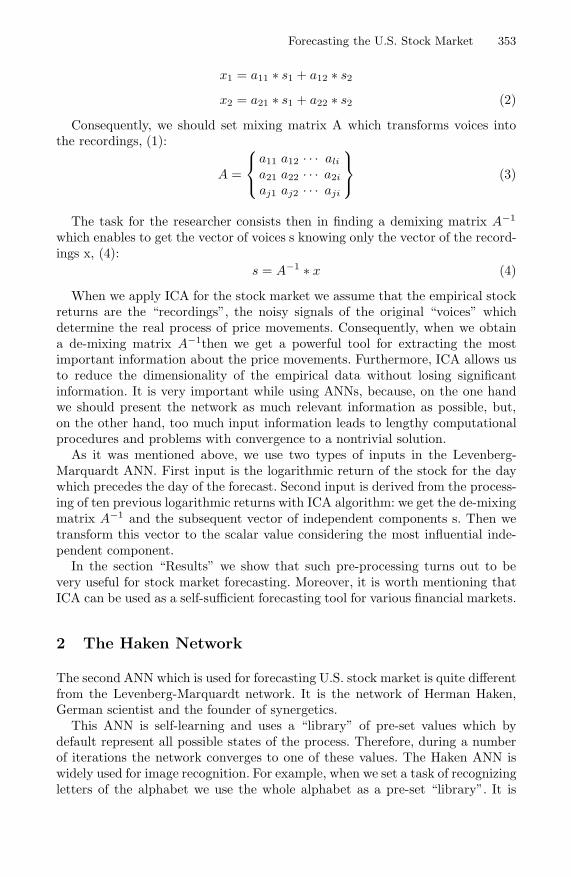
Forecasting the U.S. Stock Market 353
x1 = a11 ∗ s1 + a12 ∗ s2
x2 = a21 ∗ s1 + a22 ∗ s2 (2)
Consequently, we should set mixing matrix A which transforms voices intothe recordings, (1):
A =
⎧⎨
⎩
a11 a12 · · · ali
a21 a22 · · · a2i
aj1 aj2 · · · aji
⎫⎬
⎭ (3)
The task for the researcher consists then in finding a demixing matrix A−1
which enables to get the vector of voices s knowing only the vector of the record-ings x, (4):
s = A−1 ∗ x (4)
When we apply ICA for the stock market we assume that the empirical stockreturns are the “recordings”, the noisy signals of the original “voices” whichdetermine the real process of price movements. Consequently, when we obtaina de-mixing matrix A−1then we get a powerful tool for extracting the mostimportant information about the price movements. Furthermore, ICA allows usto reduce the dimensionality of the empirical data without losing significantinformation. It is very important while using ANNs, because, on the one handwe should present the network as much relevant information as possible, but,on the other hand, too much input information leads to lengthy computationalprocedures and problems with convergence to a nontrivial solution.
As it was mentioned above, we use two types of inputs in the Levenberg-Marquardt ANN. First input is the logarithmic return of the stock for the daywhich precedes the day of the forecast. Second input is derived from the process-ing of ten previous logarithmic returns with ICA algorithm: we get the de-mixingmatrix A−1 and the subsequent vector of independent components s. Then wetransform this vector to the scalar value considering the most influential inde-pendent component.
In the section “Results” we show that such pre-processing turns out to bevery useful for stock market forecasting. Moreover, it is worth mentioning thatICA can be used as a self-sufficient forecasting tool for various financial markets.
2 The Haken Network
The second ANN which is used for forecasting U.S. stock market is quite differentfrom the Levenberg-Marquardt network. It is the network of Herman Haken,German scientist and the founder of synergetics.
This ANN is self-learning and uses a “library” of pre-set values which bydefault represent all possible states of the process. Therefore, during a numberof iterations the network converges to one of these values. The Haken ANN iswidely used for image recognition. For example, when we set a task of recognizingletters of the alphabet we use the whole alphabet as a pre-set “library”. It is

354 S. Golovachev
obvious, because any letter which is presented to the network is essentially apart of the alphabet.
However, we aim to apply the Haken ANN for the stock market forecasting,and the situation here is much more complicated. We must choose the “library”which contains all possible states of the market. To solve this task we resortto two important assumptions. Firstly, we argue that all necessary informationwhich is needed for the forecast is contained in the returns of the stock duringten trading days before the day for which the forecast is calculated. Secondly,we assume that the using of processing techniques of the ICA and PCA, whicheventually reduces the information dimensionality, allows us to extract mostimportant and valuable information signals.
Thus, to obtain the “library” of pre-set values we use the eigenvectors of thecovariance matrix of the subsequent empirical vectors of stock returns (PCA) orthe de-mixing matrix of the empirical vectors obtained from ICA.
The network functions as follows, (5):
q∗ = q +M∑
k=1
λkvTk qvk + B
M∑
k=1
(vTk q)2(vT
k q)vk + C(qT q)q, (5)
whereq – vector of M elements which the network tries to optimize. Initially this vectoris deliberately made noisy to ignite the process of learning, thus we assume thatthe real data on the stock market is also noisy in the similar way;q∗- vector which the network finally reconstructs;V – matrix which plays a role of the “library” and contains pre-set values whichare obtained from PCA or ICA;λ – learning ratio;B – computational parameters which calibrating has an influence on the con-vergence of the network and the speed of learning.
The final forecasting signal is obtained by subtracting the empirical vectorfrom the reconstructed one.
3 Trading Rules
Now we present trading rules which were used while working with the Levenberg-Marquardt and the Haken ANNs.
Firstly, we should specify the data which we forecast. We predict price move-ments of the 30 liquid stocks of the U.S. index S&P 5001 in the period fromNovember, 7th, 2008 to May,2nd, 2010.1 We use closing prices of the following stocks: ExxonMobil, Apple, Microsoft, General
Electric, Procter&Gamble, Johnson&Johnson, Bank of America, JPMorgan Chase,Wells Fargo, IBM, Chevron, Sisco Systems, AT&T, Pfizer, Google, Coca Cola, Intel,Hewlett Packard, Wal Mart, Merck, PepsiCo, Oracle, Philip Morris International,ConocoPhillips, Verizon Communications, Schlumberger, Abbott Labs, GoldmanSachs, Mcdonalds, QUALCOMM.

Forecasting the U.S. Stock Market 355
For each trading day t we make forecast via our ANNs for each stock. Whenthe forecasts are made we range them according to their absolute value. Thefinal selection of the stocks in the virtual portfolio is based on two opposingtrading rules. According to the Rule A we select from 1 to 5 stocks with thehighest forecast value2 (note that at this step we do not know the real return ofday t which makes our forecast truly out-of-sample). According to the Rule Bwe select from 1 to 5 stocks with the lowest forecast values.
The reason for using Rule B is widely recognized phenomenon of “mean re-version” in the financial data. Thus, if Rule B is successful, then our ANN iscapable of detecting this property of the market.
The dynamics of our trade portfolio will be compared to the dynamics of theS&P 500 index and the dynamics of the portfolio if the decision-making wasbased on the simple auto-regression model (while the trading rules A and B areretained), (6):
r∗t = αt + βt ∗ rt−1, (6)
wherer∗t - forecast value of the logarithmic return of the stock for the trading day t,αt, βt-auto-regression coefficients,rt−1- logarithmic return of the stock for the trading day t-1.
4 Results
Now we present some of the results of the forecasting using the Levenberg-Marquardt and the Haken ANNs. Due to the limited space of this paper wedemonstrate here only most successful examples.
Figure 1 demonstrates relative dynamics of our virtual portfolio (red line) us-ing the Levenberg-Marquardt ANN and trading Rule B (five stocks with “worst”forecasts). Blue line is a portfolio when the decision-making is based on the auto-regression model. Blue line is the S&P 500 index. The horizontal axis is timeand t indicates trading days. The vertical axis displays the value of the portfoliowith the initial value of 1.
Figure 2 demonstrates relative dynamics of our virtual portfolio (red line)using the Haken ANN with the PCA pre-processing and trading Rule B (onestock with the “worst” forecast). Blue line is a portfolio when the decision-making is based on the auto-regression model. Green line is the S&P 500 index.The horizontal axis is time and t indicates trading days. The vertical axis displaysthe value of the portfolio with the initial value of 1.
Figure 3 demonstrates relative dynamics of our virtual portfolio (red line)using the Herman Haken ANN with the ICA pre-processing and trading Rule A(one stock with the “best” forecast). Blue line is a portfolio when the decision-making is based on the auto-regression model. Green line is the S&P 500 index.The horizontal axis is time and t indicates trading days. The vertical axis displaysthe value of the portfolio with the initial value of 1.2 Note that in this model we use only long positions, short selling is not allowed.
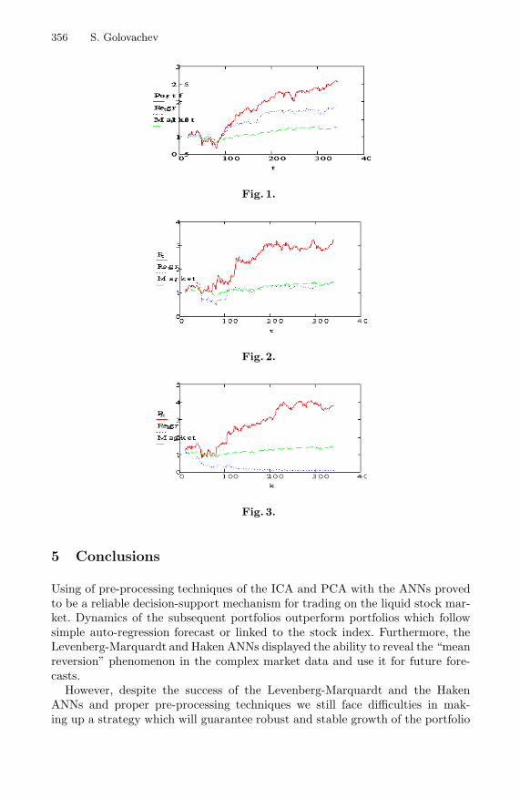
356 S. Golovachev
Fig. 1.
Fig. 2.
Fig. 3.
5 Conclusions
Using of pre-processing techniques of the ICA and PCA with the ANNs provedto be a reliable decision-support mechanism for trading on the liquid stock mar-ket. Dynamics of the subsequent portfolios outperform portfolios which followsimple auto-regression forecast or linked to the stock index. Furthermore, theLevenberg-Marquardt and Haken ANNs displayed the ability to reveal the “meanreversion” phenomenon in the complex market data and use it for future fore-casts.
However, despite the success of the Levenberg-Marquardt and the HakenANNs and proper pre-processing techniques we still face difficulties in mak-ing up a strategy which will guarantee robust and stable growth of the portfolio

Forecasting the U.S. Stock Market 357
over continuous period of time. Moreover, more theoretical research is needed tojustify the argument that it is the neural network decision-making mechanismwhich is used by traders in real life. It is also obvious that more in-depth studyis needed to explain the phenomenon of “mean reversion”. Some of these issueswill be the topics of the future research.
References
1. Back, A.D., Weigend, A.S.: A First Application of Independent Component Anal-ysis to Extracting Structure from Stock Returns. International Journal of NeuralSystems 8(5) (October 1997)
2. Bishop, C.M.: Neural Networks for Pattern Recognition, p. 483. Oxford UniversityPress, Oxford (1995)
3. Bell, J.I., Sejnowsi, T.J.: An information-maximisation approach to blind separationand blind deconvolution. Neural Computation 7(6), 1004–1034 (1995)
4. Gorriz, J.M., Puntonet, C.G., Moises Salmeron, E.W.: Lang Time Series Predictionusing ICA Algorithms. In: IEEE International Workshop on Intelligent Data Ac-quisition and Advanced Computing Systems: Technology and Applications, Lviv,Ukraine, September 8-10 (2003)
5. Hyvarinen, A., Oja, E.: Independent Component Analysis: Algorithms and Appli-cations. Neural Networks 13(4-5), 411–430 (2000)
6. Krose, B., van der Smagt, P.: An Introduction To Neural Networks, 8th edn. (Novem-ber 1996)
7. Lu, C.-J., Le, T.-S., Chiu, C.-C.: Financial time series forecasting using independentcomponent analysis and support vector regression. Decision Support Systems 47,115–125 (2009)

Empirical Study of Matrix Factorization
Methods for Collaborative Filtering
Evgeny Kharitonov
Moscow Institute of Physics and [email protected]
Abstract. Matrix factorization methods have proved to be very efficientin collaborative filtering tasks. Regularized empirical risk minimizationwith squared error loss function and L2-regularization and optimiza-tion performed via stochastic gradient descent (SGD) is one of the mostwidely used approaches.
The aim of the paper is to experimentally compare some modificationsof this approach. Namely, we compare Huber’s, smooth ε-insensitive andsquared error loss functions. Moreover, we investigate a possibility toimprove the results by applying a more sophisticated optimization tech-nique — stochastic meta-descent (SMD) instead of SGD.
Keywords: collaborative filtering, matrix factorization, loss functions.
1 Introduction
Recommender systems are widely used in online shops and services such asAmazon, Netflix, Google Video and Google News. Collaborative Filtering (CF)is one of successful approaches to build such systems. During the Netflix PrizeChallenge the matrix factorization methods attracted a lot of attention andproved to be very efficient.
A considerable portion of practical problems in the field deals with explicituser feedback: users watch movies and explicitly rate them afterwards. Our taskis to recommend some new items to the user, which he or she hasn’t seen yet.
The general idea behind factor models implies that it is possible to find user-and item-vectors which characterize the user’s tastes and items in such a waythat their dot product approximates the user’s rating of an item. After that, theitems with highest predicted user’s rating are recommended to him.
Usually these vectors are found via regularized empirical risk minimizationwith squared error loss and L2-regularization. The stochastic gradient descent(SGD) has become the most popular technique for this optimization.
The question we address is the following: Is there a better choice of a loss func-tion and an optimization algorithm, which can result in better recommendationperformance?
In order to answer the question we compare Huber’s [1] and smooth ε-insensitive [2] loss functions in comparison with squared error loss.
Stochastic meta-descent (SMD) [3] is a more elaborated algorithm which cansubstitute SGD in this combination.
S.O. Kuznetsov et al. (Eds.): PReMI 2011, LNCS 6744, pp. 358–363, 2011.c© Springer-Verlag Berlin Heidelberg 2011

Empirical Study of Matrix Factorization Methods for Collaborative Filtering 359
2 Model
Let us denote a rating matrix as X (n×r), with rows and columns correspondingto the users and items, respectively. Elements of X are real numbers or a specialsign ∗ which is used if the value of corresponding rating is unknown.
We associate vectors from Rk with i-th user and j-th item: ui and mj , corre-
spondingly.Our model is based on the idea that it is possible to find such ui and mj that
the product ui · mTj represents the i-th user rating of the j-th item:
∀i, j : Xij = ∗ Xij ≈ ui · mTj
It is convenient to formalize the task as a problem of discrepancy minimizationbetween X and its approximation U×MT in the cells with known values. In orderto do this we introduce a nonnegative loss function L. This function penalizesdivergence between predictions and actual values.
More formally, our task is to find U and M , which will minimize divergencefor the available data:
(U, M) = argmin1T
∑
i,j:Xij =∗L(Xij , ui · mT
j ),
where T is the number of observed cells in X .In order to avoid overfitting, a special term is introduced in the target function.
Usually it penalizes complex models. We use a L2 regularization term:
(U , M) = argmin
⎛
⎝ 1
T
∑
i,j:xij =∗L(xij , ui · mT
j ) + λu
∑
i
ui · uTi + λm
∑
j
mj · mTj
⎞
⎠
, where L : R × R → R+ is the loss function.
3 Loss Functions
We consider the following loss functions (they are described in [4]) L(x, x):squared error
L(x, x) =12
(x − x)2
smooth ε-insensitive loss [2]
L(x, x) = log(1 + ex−x−ε
)+ log
(1 + ex−x−ε
)
Huber’s robust loss [1]
L(x, x) =
12 (x − x)2 , |x − x| ≤ σ
σ(|x − x| − 1
2σ), otherwise
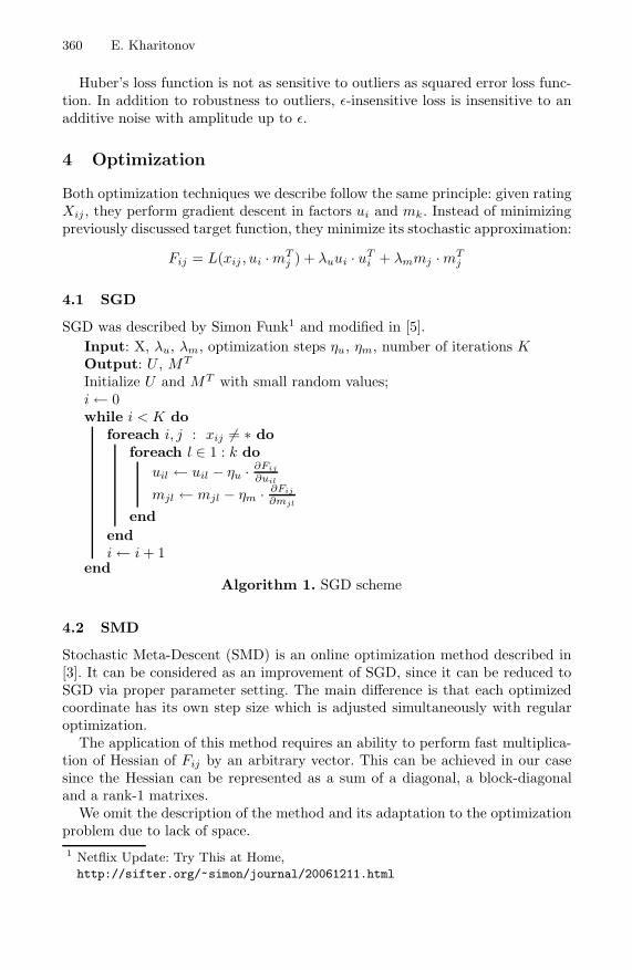
360 E. Kharitonov
Huber’s loss function is not as sensitive to outliers as squared error loss func-tion. In addition to robustness to outliers, ε-insensitive loss is insensitive to anadditive noise with amplitude up to ε.
4 Optimization
Both optimization techniques we describe follow the same principle: given ratingXij , they perform gradient descent in factors ui and mk. Instead of minimizingpreviously discussed target function, they minimize its stochastic approximation:
Fij = L(xij , ui · mTj ) + λuui · uT
i + λmmj · mTj
4.1 SGD
SGD was described by Simon Funk1 and modified in [5].Input: X, λu, λm, optimization steps ηu, ηm, number of iterations KOutput: U , MT
Initialize U and MT with small random values;i ← 0while i < K do
foreach i, j : xij = ∗ doforeach l ∈ 1 : k do
uil ← uil − ηu · ∂Fij
∂uil
mjl ← mjl − ηm · ∂Fij
∂mjl
endendi ← i + 1
endAlgorithm 1. SGD scheme
4.2 SMD
Stochastic Meta-Descent (SMD) is an online optimization method described in[3]. It can be considered as an improvement of SGD, since it can be reduced toSGD via proper parameter setting. The main difference is that each optimizedcoordinate has its own step size which is adjusted simultaneously with regularoptimization.
The application of this method requires an ability to perform fast multiplica-tion of Hessian of Fij by an arbitrary vector. This can be achieved in our casesince the Hessian can be represented as a sum of a diagonal, a block-diagonaland a rank-1 matrixes.
We omit the description of the method and its adaptation to the optimizationproblem due to lack of space.1 Netflix Update: Try This at Home,http://sifter.org/~simon/journal/20061211.html

Empirical Study of Matrix Factorization Methods for Collaborative Filtering 361
4.3 Meta-optimization
Each combination of loss function and optimization technique has several param-eters which are to be determined before model training, e.g. optimization ratesηu, ηm, regularization coefficients λu, λm, parameters of loss functions such asε and σ. However, there is no commonly adopted approach for their selection inliterature. In paper [5] a grid search is used to find optimal parameters. Anotherapproach is to use derivative-free optimization to adjust the parameters on asmall subset of available data. Similarly to [6] we use Nelder-Mead method fortuning these parameters.
The initial values of parameters in our experiments are presented in Table 1;the number of iterations used for SGD, SMD and Nelder-Mead was equal to 25.
Table 1. Initial parameters
ηu ηm λu λm σ ε μ (SMD) ν (SMD)
0.01 0.01 0.02 0.02 6.7 0.03 0.08 0.9
5 Evaluation
The authors of [7] thoroughly discuss the main evaluation criteria used in col-laborative filtering. We use three of them: RMSE (Rooted Mean Square Error),MAE (Mean Absolute Error) and Precision-N.
The first two criteria characterize how good we approximate X via productof U and MT :
RMSE =
⎛
⎝ 1T
∑
i,j:xij =∗
(xij − ui · mT
j
)2⎞
⎠
12
MAE =1T
∑
i,j:xij =∗
∣∣xij − ui · mTj
∣∣
They have several drawbacks [7]. The main problem is that they evaluate theperformance of approximation, not recommendations. For this reason, we alsouse Precision-N criterion.
A trained model can sort the items recommended to the user in the order ofdescending predicted rating.
For a particular user, Precision-N is a ratio of items with real rating above apredefined threshold t among N items with the highest predicted rating.
Precision-N = Average
(1
N|items with rating not less than t among top-N|
)
In our experiments we used Precision-5 with t = 4.

362 E. Kharitonov
0.844
0.846
0.848
0.85
0.852
0.854
0.856
0.858
10 20 30 40 50 60 70 80 90 100
RM
SE
k
Squared, SGDSquared, SMD
Smooth eps-insensitive, SGDHuber, SGD
(a) RMSE
0.66
0.665
0.67
0.675
0.68
0.685
0 10 20 30 40 50 60 70 80 90 100
MA
E
k
Squared, SGDSquared, SMD
Smooth eps-insensitive, SGDHuber, SGD
(b) MAE
0.68
0.682
0.684
0.686
0.688
0.69
0.692
0 10 20 30 40 50 60 70 80 90 100
Pre
cisi
on-5
k
Squared, SGDSquared, SMD
Smooth eps-insensitive, SGDHuber, SGD
(c) Precision-5
Fig. 1. Performance vs. k
6 Experiments
In the experiments we used an open dataset provided by MovieLens group . Itcontains about 1 million ratings of 3900 movies obtained from 6040 users.
The dataset was randomly split into 10 approximately equal parts. For eachk ∈ [1..10] the evaluation process consisted of two steps.
First of all, during the meta-optimization step the parameters that optimizetarget criterion (RMSE, MAE or Precision-5) were calculated for one part of datawhile learning on eight other parts were chosen. After that, these nine parts wereused as training data and the evaluation was performed on the previously unusedpart.
This process was repeated until all the parts were used as test sets. The resultswere averaged and are depicted in Figure 1.
We ensured that for every combination tested we used the same learning,validation and test sets, initial approximations for U and M (for fixed k) andthe number of meta-optimization and optimization iterations.
The source code is available on http://github.com/n0mad/Demoniac.

Empirical Study of Matrix Factorization Methods for Collaborative Filtering 363
7 Discussion
As seen from figures, loss functions that are close to L2 (Huber’s and squared er-ror loss) unsurprisingly result in a better RMSE performance. Similarly, smoothε-insensitive loss (which approximates L1 loss) achieves a better MAE perfor-mance.
More importantly, our experiment has shown that none of the considered mod-ifications did significantly improve Precision-5 in comparison with the standardapproach. Thus, taking into consideration simplicity of implementation and lackof additional parameters SGD with L2 loss and regularization seems to be thebest choice.
References
1. Huber, P.J.: Robust statistics. Wiley, New York (1981)2. Dekel, O., Shalev-Shwartz, S., Singer, Y.: Smooth e-intensive regression by loss
symmetrization. In: COLT, pp. 433–447 (2003)3. Bray, M., Koller-meier, E., Muller, P., Van Gool, L., Schraudolph, N.N.: 3d hand
tracking by rapid stochastic gradient descent using a skinning model. In: CVMP,pp. 59–68 (2004)
4. Karatzoglou, A., Smola, A., Weimer, M.: Collaborative filtering on a budget. In:AISTATS, vol. 9, pp. 389–396 (2010)
5. Takacs, G., Pilaszy, I., Nemeth, B., Tikk, D.: Scalable collaborative filtering ap-proaches for large recommender systems. Journal of Machine Learning Research 10,623–656 (2009)
6. Cohen, G., Ruch, P., Hilario, M.: Model selection for support vector classifiers viadirect simplex search. In: FLAIRS Conference, pp. 431–435 (2005)
7. Herlocker, J.L., Konstan, J.A., Terveen, L.G., Riedl, J.T.: Evaluating collaborativefiltering recommender systems. ACM Transactions on Information Systems 22, 5–53(2004)
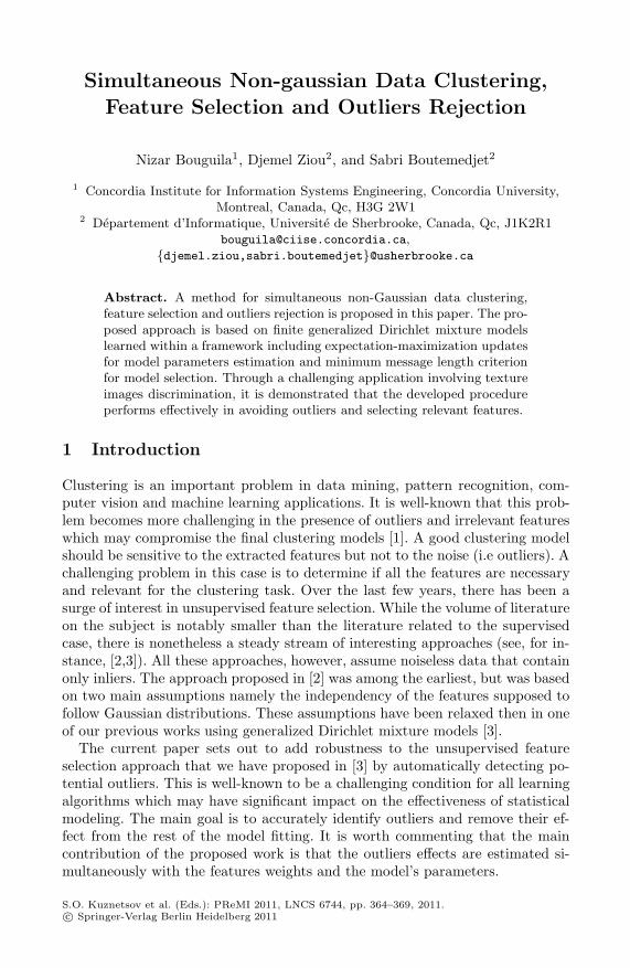
Simultaneous Non-gaussian Data Clustering,
Feature Selection and Outliers Rejection
Nizar Bouguila1, Djemel Ziou2, and Sabri Boutemedjet2
1 Concordia Institute for Information Systems Engineering, Concordia University,Montreal, Canada, Qc, H3G 2W1
2 Departement d’Informatique, Universite de Sherbrooke, Canada, Qc, [email protected],
djemel.ziou,[email protected]
Abstract. A method for simultaneous non-Gaussian data clustering,feature selection and outliers rejection is proposed in this paper. The pro-posed approach is based on finite generalized Dirichlet mixture modelslearned within a framework including expectation-maximization updatesfor model parameters estimation and minimum message length criterionfor model selection. Through a challenging application involving textureimages discrimination, it is demonstrated that the developed procedureperforms effectively in avoiding outliers and selecting relevant features.
1 Introduction
Clustering is an important problem in data mining, pattern recognition, com-puter vision and machine learning applications. It is well-known that this prob-lem becomes more challenging in the presence of outliers and irrelevant featureswhich may compromise the final clustering models [1]. A good clustering modelshould be sensitive to the extracted features but not to the noise (i.e outliers). Achallenging problem in this case is to determine if all the features are necessaryand relevant for the clustering task. Over the last few years, there has been asurge of interest in unsupervised feature selection. While the volume of literatureon the subject is notably smaller than the literature related to the supervisedcase, there is nonetheless a steady stream of interesting approaches (see, for in-stance, [2,3]). All these approaches, however, assume noiseless data that containonly inliers. The approach proposed in [2] was among the earliest, but was basedon two main assumptions namely the independency of the features supposed tofollow Gaussian distributions. These assumptions have been relaxed then in oneof our previous works using generalized Dirichlet mixture models [3].
The current paper sets out to add robustness to the unsupervised featureselection approach that we have proposed in [3] by automatically detecting po-tential outliers. This is well-known to be a challenging condition for all learningalgorithms which may have significant impact on the effectiveness of statisticalmodeling. The main goal is to accurately identify outliers and remove their ef-fect from the rest of the model fitting. It is worth commenting that the maincontribution of the proposed work is that the outliers effects are estimated si-multaneously with the features weights and the model’s parameters.
S.O. Kuznetsov et al. (Eds.): PReMI 2011, LNCS 6744, pp. 364–369, 2011.c© Springer-Verlag Berlin Heidelberg 2011
Simultaneous Non-gaussian Data Clustering 365
The rest of this paper is organized as follows. After introducing our modeland justifying its use and how it can be learned in Section 2, we illustrate theproposed approach on a real application which concerns texture images discrim-ination in Section 3. Finally, we conclude the paper with a summary of the workin Section 4.
2 Unsupervised Feature Selection and Outliers Rejection
2.1 The Model
Let us consider a data set of N vectors X = X1, . . . , XN, where each Xi =(Xi1, . . . , XiD) is a D-dimensional vector of features representing a given image,for instance. Set of vectors generally contains examples that belong to manyclusters and can be modeled by a finite mixture of distributions
p(Xi|Θ) =M∑
j=1
pjp(Xi|θj) (1)
where pj > 0, are the mixing proportions, M is the number of mixture compo-nents, and Θ = P = (p1, . . . , pM ),θ = (θ1, . . . , θM) is the set of parametersin the mixture model. A critical problem in this case is the choice of the prob-ability density function p(Xi|θj) to represent each component. In [3], we haveshown that the generalized Dirichlet distribution offers the unusual luxury thatby a simple transformation we go from one space to another one where all thevariables are independent and follow Beta distributions [4,5]. This allows us toeasily formalize the fact that different features may have different weights byapproximating a generalized Dirichlet mixture as following [3]
p(X i|Θ) =M∑
j=1
pj
D∏
d=1
(ρdp(Xid|αjd, βjd) + (1 − ρd)p(Xid|αd, βd)
)(2)
where Θ = P , ρd, αjd, βjd, αd, βd is the set of all the model parame-ters, ρd represents the probability that the dth feature is relevant for clustering,p(Xid|αjd, βjd) is a Beta distribution that represents a feature Xid when it isrelevant, and p(Xid|αd, βd) is an univariate Beta with parameters αd, βd and canbe viewed as a common background distribution to explain nonsalient features.It is noteworthy that in the previous model no knowledge is available as to whichvector Xi is not representative (i.e. an outlier) and then is not really generatedfrom our assumed statistical model. Model selection, feature selection and pa-rameters estimation are generally dramatically affected by outliers. Thus, it iscrucial to extend the model in Eq. 2 to handle outliers. We approach this prob-lem by incorporating an auxiliary outlier component to which we associate auniform density 1 into the model:1 Supposing that the outliers follow a uniform distribution is a reasonable common
assumption that have been considered in several computer vision and pattern recog-nition applications (see, for instance, [6,7]).

366 N. Bouguila, D. Ziou, and S. Boutemedjet
p(Xi|Θ) =M∑
j=1
pj
D∏
d=1
(ρdp(Xid|αjd, βjd) + (1 − ρd)p(Xid|αd, βd)
)+ pM+1U(Xi)
(3)where pM+1 = 1 −∑M
j=1 pj is the probability that Xi was not generated bythe central mixture model and U (X i) is a uniform distribution common for alldata to model isolated vectors which are not in any of the M clusters and whichshow significantly less differentiation among clusters. The previous model canbe viewed as a way to robustify unsupervised feature selection to learn the rightmeaning from the right observations (i.e inliers). Notice that when pM+1 = 0the outlier component is removed and the previous equation is reduced to Eq. 2.
2.2 Model Learning
A well-known approach for unknown parameters estimation is the techniqueof maximum likelihood (ML) which properties have been extensively examinedin the past. Using ML the parameters are estimated by maximizing the log-likelihood function as following
Θ = arg maxΘ
log p(X|Θ) =
N∑
i=1
log[ M∑
j=1
(pj
D∏
d=1
(ρdpjd(Xid) + (1 − ρd)p(Xid)
))
+ pM+1U(Xi)]
(4)
where pjd(Xid) = p(Xid|αjd, βjd) and p(Xid) = p(Xid|αd, βd), which gives us
pj =∑N
i=1 p(j|Xi)N
j = 1, . . . , M + 1 (5)
where
p(j|X i) =
⎧⎪⎪⎪⎪⎪⎨
⎪⎪⎪⎪⎪⎩
pj∏D
d=1
(ρdpjd(Xid)+(1−ρd)p(Xid)
)
∑Mj=1
(pj∏
Dd=1
(ρdpjd(Xid)+(1−ρd)p(Xid)
))+pM+1U(X i)
if j = 1, . . . , M
pM+1U(X i)
∑Mj=1
(pj∏D
d=1
(ρdpjd(Xid)+(1−ρd)p(Xid)
))+pM+1U(X i)
if j = M + 1(6)
is the posterior probability that a vector Xi will be considered as an inlier andthen assigned to a cluster j, j = 1, . . . , M or as an outlier and then affected tocluster M + 1 which allows to safeguard against erroneous feature selection. De-tails about the estimation of the other parameters namely αjd, βjd, αd, βd andρd can be found in [3]. It is desirable to determine the simplest model that canexplain the data accurately. It is noteworthy that the simplicity is measured inour case by the number of mixture components and the number of relevant fea-tures. The simplest model can be viewed as the one that maximizes the messagelength, to reach an acceptable balance between model complexity and goodness

Simultaneous Non-gaussian Data Clustering 367
of fit. Details and discussions about the computation of the message length canbe found in [4,3].
Algorithm
For each candidate value of M :
1. Set ρd ← 0.5, d = 1, . . . , D, j = 1, . . . , M and initialization of the rest ofparameters 2.
2. Iterate the two following steps until convergence:(a) E-Step: Update p(j|Xn) using Eq. 6.(b) M-Step: Update the pj , ρd, βjd, αjd, βd and αd as proposed in [3].
3. Calculate the associated message length [3].4. Select the optimal model that yields the smallest message length.
3 Experimental Results: Texture Discrimination
The problem of texture discrimination has been the subject of several studies inthe past (see, for instance, [8,9]). Several texture descriptors have been proposed[10] and applied to several problems such as industrial surface inspection andcontent-based image retrieval. We shall not elaborate further on the different ap-proaches that have been proposed to model textures which is clearly beyond thescope of this paper. Rather we focus on an important texture feature extractionapproach that has received a lot of attention recently. This approach is based onthe representation of texture using visual dictionary obtained through the quan-tization of the appearance of local regions, described by local features, whichgives characteristic texture elements generally called textons (see, for instance,[11]).
For our experimental evaluation, we use the KTH-TIPS [12] texture data setwhich is composed of 10 texture classes with 81 images per class (see Fig. 1).We add to this data set 20 different images, taken from different classes of theMIT vistex texture data set, which will be considered as outliers (see Fig. 2). Animportant step in our application is the extraction of local features to describethe textures. In our case we use the approach proposed in [11] which uses n× npixel compact neighborhoods as image descriptors. Using this approach each tex-ture pixel is described by an n2-dimensional vector which represents the pixelintensities of its n × n square neighborhood. Following [11], we use n = 7, thus
Fig. 1. Examples of images from the 10 different classes in the KTH-TIPS data set
2 The initialization is based on the K-Means algorithm and the method of momentsby considering that M + 1 clusters are present in the data.

368 N. Bouguila, D. Ziou, and S. Boutemedjet
Fig. 2. Sample images from the Vistex data set
each pixel is represented by a 49-dimensional vector. Then, we construct a globaltexton vocabulary via the clustering of the different descriptors. In particular,we extract 10 textons using K-Means (i.e. the textons are actually the K-Meanscluster centers) for each texture class and then concatenate the textons of thedifferent classes to form the visual vocabulary. Thus, the vocabulary size is 100.Once the vocabulary of textons is built, each texture image can be representedthen by a vector of frequencies which we normalize.
Evaluation results by considering different clustering scenarios and by com-paring generalized Dirichlet mixture (GDM) and Gaussian mixture (GM) aresummarized in table 1. It is noteworthy that in both cases (GDM or GM), wewere able to find the exact number of clusters only when we have rejected theoutliers. According to the results in table 1 it is clear that the GDM outper-forms the GM which is actually an expected result taking into account the factthat the features vectors are proportional vectors for which the GDM is one ofthe best choices. It is clear also that feature selection improves the clusteringperformance especially when combined with outliers rejection.
Table 1. Clustering results for the KTH-TIPS data set by considering different sce-narios. Clust denotes clustering without feature selection and outliers rejection, FSdenotes feature selection and OR denotes outliers rejection.
Clust Clust+FS Clust+OR Clust+FS+OR
GDM 72.23% 74.88% 74.31% 76.77%GM 68.76% 70.13% 70.02% 72.22%
4 Conclusion
The goal of the proposed work is to tackle simultaneously two of the chief obsta-cles to effective clustering namely the presence of outliers and irrelevant features.Our approach is based on extending the unsupervised feature selection techniquethat we have previously proposed in [3] to take into account outliers. The meritsof the proposed framework have been shown via the clustering of texture images.
Acknowledgment
The completion of this research was made possible thanks to the Natural Sciencesand Engineering Research Council of Canada (NSERC).

Simultaneous Non-gaussian Data Clustering 369
References
1. Fayyad, U., Piatetsky-Shapiro, G., Smyth, P.: Knowledge Discovery and Data Min-ing: Towards a Unifying Framework. In: Proc. of the Annual ACM SIGKDD Con-ference on Knowledge Discovery and Data Mining (KDD), pp. 82–88 (1996)
2. Law, M.H.C., Figueiredo, M.A.T., Jain, A.K.: Simultaneous Feature Selection andClustering Using Mixture Models. IEEE Transactions on Pattern Analysis andMachine Intelligence 26(9), 1154–1166 (2004)
3. Boutemedjet, S., Bouguila, N., Ziou, D.: A Hybrid Feature Extraction Selection Ap-proach for High-Dimensional Non-Gaussian Data Clustering. IEEE Transactionson Pattern Analysis and Machine Intelligence 31(8), 1429–1443 (2009)
4. Bouguila, N., Ziou, D.: High-Dimensional Unsupervised Selection and Estimationof a Finite Generalized Dirichlet Mixture Model Based on Minimum MessageLength. IEEE Transactions on Pattern Analysis and Machine Intelligence 29(10),1716–1731 (2007)
5. Bouguila, N., Ziou, D.: A New Approach for High-Dimensional UnsupervisedLearning: Applications to Image Restoration. In: Pal, S.K., Bandyopadhyay, S.,Biswas, S. (eds.) PReMI 2005. LNCS, vol. 3776, pp. 200–205. Springer, Heidelberg(2005)
6. Williams, C.K.I., Titsias, M.K.: Greedy Learning of Multiple Objects in Imagesusing Robust Statistics and Factorial Learning. Neural Computation 16(5), 1039–1062 (2003)
7. Sudderth, E.B., Torralba, A., Freeman, W.T., Wilsky, A.S.: Depth from FamiliarObjects: A Hierarchical Model for 3D Scenes. In: Proc. of the IEEE Conference onComputer Vision and Pattern Recognition (CVPR), pp. 2410–2417 (2006)
8. Luettgen, M.R., Willsky, A.S.: Likelihood Calculation for a Class of MultiscaleStochastic Models, with Application to Texture Discrimination. IEEE Transactionson Image Processing 4(2), 194–207 (1995)
9. Ojala, T., Valkealahti, K., Oja, E., Pietikainen, M.: Texture Discrimination withMultidimensional Distributions of Signed Gray-Level Differences. Pattern Recog-nition 34, 727–739 (2001)
10. Ojala, T., Maenpaa, T., Viertola, J., Kyllonen, J., Pietikainen, M.: Empirical Eval-uation of MPEG-7 Texture Descriptors with a Large-Scale Experiment. In: Proc.of the 2nd International Workshop on Texture Analysis and Synthesis, pp. 99–102(2002)
11. Varma, A., Zisserman, A.: Texture classification: are filter banks necessary? In.In: Proc. of the IEEE Conference on Computer Vision and Pattern Recognition(CVPR), pp. 691–698 (2003)
12. Hayman, E., Caputo, B., Fritz, M., Eklundh, J.-O.: On the significance of real-world conditions for material classification. In: Pajdla, T., Matas, J(G.) (eds.)ECCV 2004. LNCS, vol. 3024, pp. 253–266. Springer, Heidelberg (2004)

Simultaneous Clustering: A Survey
Malika Charrad and Mohamed Ben Ahmed
National School of Computer ScienceManouba University, Tunisia
malika.charrad,[email protected]
http://www.riadi.rnu.tn/
Abstract. Although most of the clustering literature focuses on one-sided clustering algorithms, simultaneous clustering has recently gainedattention as a powerful tool that allows to circumvent some limitationsof classical clustering approach. Simultaneous clustering methods per-form clustering in the two dimensions simultaneously. In this paper, weintroduce a large number of existing simultaneous clustering approachesapplied in bioinformatics as well as in text mining, web mining and in-formation retrieval and classify them in accordance with the methodsused to perform the clustering and the target applications.
Keywords: Simultaneous clustering, Biclusters, Block clustering.
1 Introduction
Simultaneous clustering, usually designated by biclustering, co-clustering, 2-wayclustering or block clustering, is an important technique in two-way data anal-ysis. A number of algorithms that perform simultaneous clustering on rows andcolumns of a matrix have been proposed to date. The goal of simultaneous clus-tering is to find sub-matrices, which are subgroups of rows and subgroups ofcolumns that exhibit a high correlation. This type of algorithms has been pro-posed and used in many fields, such as bioinformatique [23], web mining [8], textmining [3] and social network analysis [18]. A wide range of different articleswere published dealing with different kinds of algorithms and methods of simul-taneous clustering. Comparisons of several biclustering algorithms can be found,in [23] and [27]. However, these comprehensive surveys focus only on algorithmsused to genetic data analysis. In this paper, we give a brief description of alarge number of existing approaches to biclustering including approaches basedon mixture model, and those based on information theory.
2 Simultaneous Clustering Problem
Clustering is the grouping together of similar subjects. Standard clustering tech-niques consider the value of each point in all dimensions, in order to form groupof similar points. This type of one-way clustering techniques is based on similar-ity between subjects across all variables.
S.O. Kuznetsov et al. (Eds.): PReMI 2011, LNCS 6744, pp. 370–375, 2011.c© Springer-Verlag Berlin Heidelberg 2011
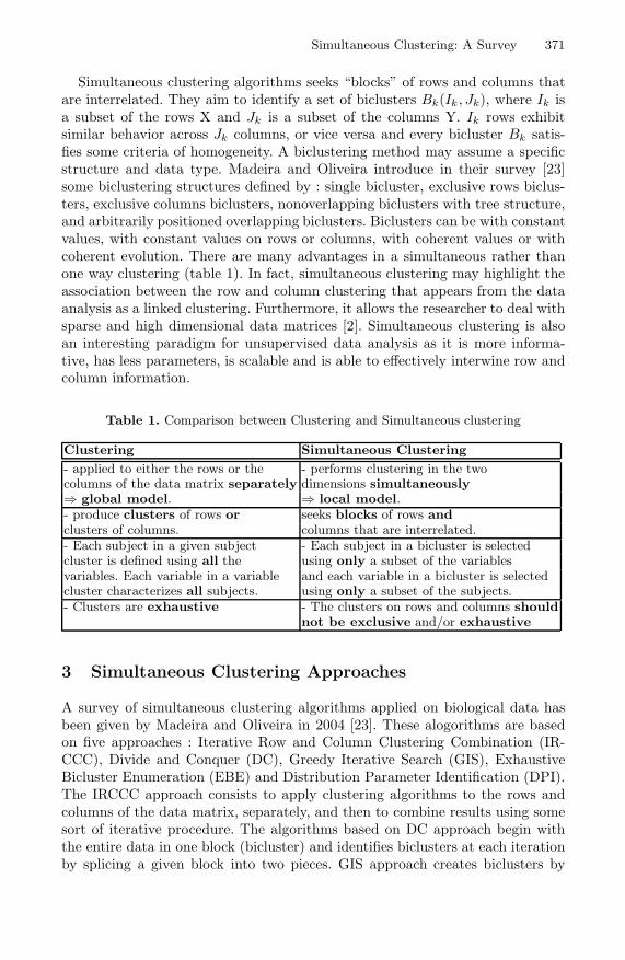
Simultaneous Clustering: A Survey 371
Simultaneous clustering algorithms seeks “blocks” of rows and columns thatare interrelated. They aim to identify a set of biclusters Bk(Ik , Jk), where Ik isa subset of the rows X and Jk is a subset of the columns Y. Ik rows exhibitsimilar behavior across Jk columns, or vice versa and every bicluster Bk satis-fies some criteria of homogeneity. A biclustering method may assume a specificstructure and data type. Madeira and Oliveira introduce in their survey [23]some biclustering structures defined by : single bicluster, exclusive rows biclus-ters, exclusive columns biclusters, nonoverlapping biclusters with tree structure,and arbitrarily positioned overlapping biclusters. Biclusters can be with constantvalues, with constant values on rows or columns, with coherent values or withcoherent evolution. There are many advantages in a simultaneous rather thanone way clustering (table 1). In fact, simultaneous clustering may highlight theassociation between the row and column clustering that appears from the dataanalysis as a linked clustering. Furthermore, it allows the researcher to deal withsparse and high dimensional data matrices [2]. Simultaneous clustering is alsoan interesting paradigm for unsupervised data analysis as it is more informa-tive, has less parameters, is scalable and is able to effectively interwine row andcolumn information.
Table 1. Comparison between Clustering and Simultaneous clustering
Clustering Simultaneous Clustering
- applied to either the rows or the - performs clustering in the twocolumns of the data matrix separately dimensions simultaneously⇒ global model. ⇒ local model.- produce clusters of rows or seeks blocks of rows andclusters of columns. columns that are interrelated.- Each subject in a given subject - Each subject in a bicluster is selectedcluster is defined using all the using only a subset of the variablesvariables. Each variable in a variable and each variable in a bicluster is selectedcluster characterizes all subjects. using only a subset of the subjects.- Clusters are exhaustive - The clusters on rows and columns should
not be exclusive and/or exhaustive
3 Simultaneous Clustering Approaches
A survey of simultaneous clustering algorithms applied on biological data hasbeen given by Madeira and Oliveira in 2004 [23]. These alogorithms are basedon five approaches : Iterative Row and Column Clustering Combination (IR-CCC), Divide and Conquer (DC), Greedy Iterative Search (GIS), ExhaustiveBicluster Enumeration (EBE) and Distribution Parameter Identification (DPI).The IRCCC approach consists to apply clustering algorithms to the rows andcolumns of the data matrix, separately, and then to combine results using somesort of iterative procedure. The algorithms based on DC approach begin withthe entire data in one block (bicluster) and identifies biclusters at each iterationby splicing a given block into two pieces. GIS approach creates biclusters by
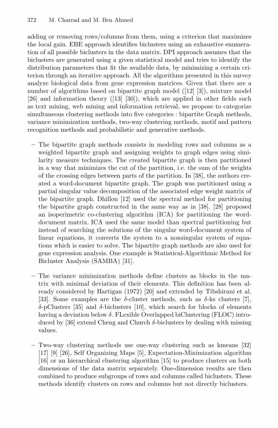
372 M. Charrad and M. Ben Ahmed
adding or removing rows/columns from them, using a criterion that maximizesthe local gain. EBE approach identifies biclusters using an exhaustive enumera-tion of all possible biclusters in the data matrix. DPI approach assumes that thebiclusters are generated using a given statistical model and tries to identify thedistribution parameters that fit the available data, by minimizing a certain cri-terion through an iterative approach. All the algorithms presented in this surveyanalyze biological data from gene expression matrices. Given that there are anumber of algorithms based on bipartite graph model ([12] [3]), mixture model[26] and information theory ([13] [30]), which are applied in other fields suchas text mining, web mining and information retrieval, we propose to categorizesimultaneous clustering methods into five categories : bipartite Graph methods,variance minimization methods, two-way clustering methods, motif and patternrecognition methods and probabilistic and generative methods.
– The bipartite graph methods consists in modeling rows and columns as aweighted bipartite graph and assigning weights to graph edges using simi-larity measure techniques. The created bipartite graph is then partitionedin a way that minimizes the cut of the partition, i.e. the sum of the weightsof the crossing edges between parts of the partition. In [38], the authors cre-ated a word-document bipartite graph. The graph was partitioned using apartial singular value decomposition of the associated edge weight matrix ofthe bipartite graph. Dhillon [12] used the spectral method for partitioningthe bipartite graph constructed in the same way as in [38]. [28] proposedan isoperimetric co-clustering algorithm (ICA) for partitioning the word-document matrix. ICA used the same model than spectral partitioning butinstead of searching the solutions of the singular word-document system oflinear equations, it converts the system to a nonsingular system of equa-tions which is easier to solve. The bipartite graph methods are also used forgene expression analysis. One example is Statistical-Algorithmic Method forBicluster Analysis (SAMBA) [31].
– The variance minimization methods define clusters as blocks in the ma-trix with minimal deviation of their elements. This definition has been al-ready considered by Hartigan (1972) [20] and extended by Tibshirani et al.[33]. Some examples are the δ-cluster methods, such as δ-ks clusters [7],δ-pClusters [35] and δ-biclusters [10], which search for blocks of elementshaving a deviation below δ. FLexible Overlapped biClustering (FLOC) intro-duced by [36] extend Cheng and Church δ-biclusters by dealing with missingvalues.
– Two-way clustering methods use one-way clustering such as kmeans [32][17] [9] [26], Self Organizing Maps [5], Expectation-Minimization algorithm[16] or an hierarchical clustering algorithm [15] to produce clusters on bothdimensions of the data matrix separately. One-dimension results are thencombined to produce subgroups of rows and columns called biclusters. Thesemethods identify clusters on rows and columns but not directly biclusters.
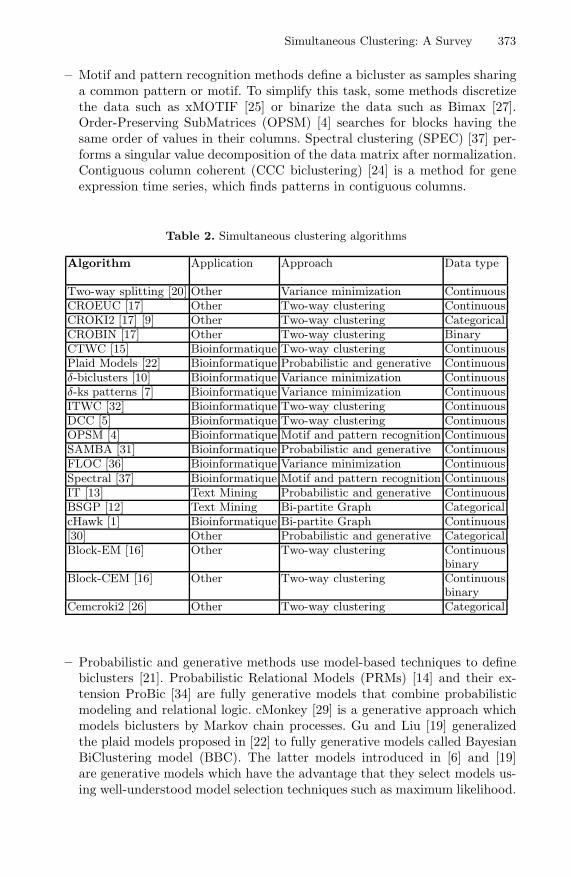
Simultaneous Clustering: A Survey 373
– Motif and pattern recognition methods define a bicluster as samples sharinga common pattern or motif. To simplify this task, some methods discretizethe data such as xMOTIF [25] or binarize the data such as Bimax [27].Order-Preserving SubMatrices (OPSM) [4] searches for blocks having thesame order of values in their columns. Spectral clustering (SPEC) [37] per-forms a singular value decomposition of the data matrix after normalization.Contiguous column coherent (CCC biclustering) [24] is a method for geneexpression time series, which finds patterns in contiguous columns.
Table 2. Simultaneous clustering algorithms
Algorithm Application Approach Data type
Two-way splitting [20] Other Variance minimization ContinuousCROEUC [17] Other Two-way clustering ContinuousCROKI2 [17] [9] Other Two-way clustering CategoricalCROBIN [17] Other Two-way clustering BinaryCTWC [15] Bioinformatique Two-way clustering ContinuousPlaid Models [22] Bioinformatique Probabilistic and generative Continuousδ-biclusters [10] Bioinformatique Variance minimization Continuousδ-ks patterns [7] Bioinformatique Variance minimization ContinuousITWC [32] Bioinformatique Two-way clustering ContinuousDCC [5] Bioinformatique Two-way clustering ContinuousOPSM [4] Bioinformatique Motif and pattern recognition ContinuousSAMBA [31] Bioinformatique Probabilistic and generative ContinuousFLOC [36] Bioinformatique Variance minimization ContinuousSpectral [37] Bioinformatique Motif and pattern recognition ContinuousIT [13] Text Mining Probabilistic and generative ContinuousBSGP [12] Text Mining Bi-partite Graph CategoricalcHawk [1] Bioinformatique Bi-partite Graph Continuous[30] Other Probabilistic and generative CategoricalBlock-EM [16] Other Two-way clustering Continuous
binaryBlock-CEM [16] Other Two-way clustering Continuous
binaryCemcroki2 [26] Other Two-way clustering Categorical
– Probabilistic and generative methods use model-based techniques to definebiclusters [21]. Probabilistic Relational Models (PRMs) [14] and their ex-tension ProBic [34] are fully generative models that combine probabilisticmodeling and relational logic. cMonkey [29] is a generative approach whichmodels biclusters by Markov chain processes. Gu and Liu [19] generalizedthe plaid models proposed in [22] to fully generative models called BayesianBiClustering model (BBC). The latter models introduced in [6] and [19]are generative models which have the advantage that they select models us-ing well-understood model selection techniques such as maximum likelihood.

374 M. Charrad and M. Ben Ahmed
Costa et al. [11] introduced a hierarchical model-based co-clustering algo-rithm. In their method the co-occurrence matrix is characterized in proba-bilistic terms, by estimating the joint distribution between rows and columns.
The table 2 presents main simultaneous clustering algorithms dealing withcontinuous, binary or categorical data, the approach they are based on and thedomain of application.
4 Conclusion
The survey presented in this work can be used by the interested researcher as agood starting point to learn and apply some of the many techniques proposedin the last few years, and some of the older ones. Many interesting directions forfuture research have been uncovered by this review work, like the validation ofbiclustering methods and the statistical significance of biclusters.
References
1. Ahmad, W., Khokhar, A.: cHawk: an efficient biclustering algorithm based onbipartite graph crossing minimization. VLDB. ACM, New York (2007)
2. Balbi, S., Miele, R., Scepi, G.: Clustering of documents from a two-way viewpoint.In: 10th Int. Conf. on Statistical Analysis of Textual Data (2010)
3. Bichot, C.E.: Co-clustering documents and words by minimizing the normalizedcut objective function. JMMA 9, 131–147 (2010)
4. Ben-Dor, A., Chor, B., Karp, R.: Discovering local structure in gene expressiondata: The order–preserving submatrix problem. J. of Comput. Biol. 10, 373–384(2003)
5. Busygin, S., Jacobsen, G., Kramer, E.: Double conjugated clustering applied toleukemia microarray data. In: 2nd SIAM Int. Conf. on Data Mining (2002)
6. Caldas, J., Kaski, S.: Bayesian biclustering with the plaid model. In: IEEE Intern.Workshop on Machine Learning for Signal Processing, pp. 291–296 (2008)
7. Califano, A., Stolovitzky, G., Tu, Y.: Analysis of gene expression microarays forphenotype classification. In: Int. Conf. on Computational Molecular Biology (2000)
8. Charrad, M., Lechevallier, Y., Ahmed, M.b., Saporta, G.: Block Clustering forWeb Pages Categorization. In: Corchado, E., Yin, H. (eds.) IDEAL 2009. LNCS,vol. 5788, pp. 260–267. Springer, Heidelberg (2009)
9. Charrad, M.: une approche generique pour l’analyse croisant usage et contenu desites Web par des methodes de bipartitionnement. PhD Thesis, Paris (2010)
10. Cheng, Y., Church, G.M.: Biclustering of expression data. In: 8th Int. Conf. onIntelligent Systems for Molecular Biology, pp. 93–103 (2000)
11. Costa, G., Manco, G., Ortale, R.: A hierarchical model-based approach to co-clustering high-dimensional data. In: ACM sym. on App. comput., pp. 886–890(2008)
12. Dhillon, I.S.: Co-clustering documents and words using bipartite spectral graphpartitioning. In: 7th ACM SIGKDD 2001, California, pp. 269–274 (2001)
13. Dhillon, I.S., Mallela, S., Modha, D.S.: Information-theoretic co-clustering. In:ACM SIGKDD, pp. 89–98. ACM, Washington DC (2003)
14. Getoor, L., Friedman, N., Koller, D., Taskar, B.: Learning probabilistic models oflink structure. J. Mach. Learn. Res. 3, 679–707 (2002)
Simultaneous Clustering: A Survey 375
15. Getz, G., Levine, E., Domany, E.: Coupled two-way clustering analysis of genemicroarray data. Proc. of the Natural Academy of Sciences USA (2000)
16. Govaert, G., Nadif, M.: Clustering with block mixture models. J. of the PatternRecognition, 463–473 (2003)
17. Govaert, G.: Classification croisee. Th. de doctorat d’Etat, Paris (1983)18. Grimal, C., Bisson, G.: Classification a partir d’une collection de matrices.
CAp2010 (2010)19. Gu, J.: Bayesian biclustering of gene expression data. BMC Genomics (2008).20. Hartigan, J.A.: Direct clustering of a data matrix. J. of American Statistical As-
sociation 67(337), 123–129 (1972)21. Hochreiter, S., Bodenhofer, U., Heusel, M., Mayr, A.: FABIA: factor analysis for
bicluster acquisition. Bioinformatics journal 26(12), 1520–1527 (2010)22. Lazzeroni, L., Owen, A.: Plaid models for gene expression data. Technical report,
Stanford University (2002)23. Madeira, S.C., Oliveira, A.L.: Biclustering Algorithms for Biological Data Analysis:
A Survey. IEEE/ACM Trans. on Comp. Biol. and Bioinfor., 24–45 (2004)24. Madeira, S.C., Teixeira, M.C.: Identification of regulatory modules in time series
gene expression data using a linear time biclustering algorithm. IEEE ACM (2010)25. Murali, T.M., Kasif, S.: Extracting conserved gene expression motifs from gene
expression data. In: Pacific Sym. on Biocomputing, Hawaii, USA, pp. 77–88 (2003)26. Nadif, M., Govaert, G.: Block clustering of contingency table and mixture model.
In: Famili, A.F., Kok, J.N., Pena, J.M., Siebes, A., Feelders, A. (eds.) IDA 2005.LNCS, vol. 3646, pp. 249–259. Springer, Heidelberg (2005)
27. Prelic, A., Bleuler, S., Zimmermann, P.: A systematic comparison and evaluationof biclustering methods for gene expression data. Bioinformatics, 122–129 (2006)
28. Rege, M., Dong, M.: Co-clustering Documents and Words Using Bipartite Isoperi-metric Graph Partitioning. In: 6th IEEE Int. Conf. on Data Mining, pp. 532–541(2006)
29. Reiss, D.J.: Integrated biclustering of heterogeneous genome-wide datasets for theinference of global regulatory networks. BMC Bioinfor., 280–302 (2006)
30. Robardet, C.: Contribution a la classification non supervisee : proposition d’unemethode de bi-partitionnement, PhD Thesis, Claude Bernard University (2002).
31. Tanay, A., Sharan, R., Shamir, R.: Biclustering Algorithms: A Survey. In: Aluru,S. (ed.) Handbook of Comp. Molecular Biology, Chapman, Boca Raton (2004)
32. Tang, C., Zhang, L.A.: Interrelated two-way clustering: an unsupervised approachfor gene expression data analysis. In: IEEE Int. Sym. on Bioinfo. and Bioeng.(2001)
33. Tibshirani, R., Hastie, T., Eisen, M.: Clustering methods for the analysis of DNAmicroarray data. Technical report, Stanford University (1999)
34. Van den, B.T.: Robust Algorithms for Inferring Regulatory Networks Based onGene Expression Measurements. PhD Thesis (2009)
35. Wang, H., Wang, W., Yang, J., Yu, P.S.: Clustering by pattern similarity in largedata sets. In: ACM SIGMOD Int. Conf. on Management of Data, pp. 394–405(2002)
36. Yang, J., Wang, H., Wang, W., Yu, P.S.: An improved biclustering method foranalyzing gene expression profiles. Int. J. on Art. Int. Tools, 771–790 (2005)
37. Klugar, Y., Basri, R., Chang, J.T., Gerstein, M.: Spectral biclustering of microarraydata: coclustering genes and conditions. Genome Research 13, 703–716 (2003)
38. Zha, H., He, X., Ding, C., Simon, H., Gu, M.: Bipartite Graph Partitioning andData Clustering. In: ACM Conf. on Inf. and Knowledge Management, pp. 25–32(2001)

Analysis of Centrality Measures of Airport
Network of India
Manasi Sapre and Nita Parekh
International Institute of Information Technology, Hyderabad 500032, [email protected], [email protected]
Abstract. In this paper we analyze the topological properties of airportnetwork of India (ANI) using graph theoretic approach. We show thatsuch an analysis can be useful not only in planning the infrastructureand growth of the air-traffic connectivity, but also in managing the flowof transportation during emergencies such as accidental failure of theairport, close down of the airport due to unexpected climate changes,terrorist attacks, etc. Knowledge of the connectivity pattern and load onvarious routes can also help in making judicious decisions for reductionof flights to contain the spread of the infectious disease.
Keywords: graph theory, centrality measures, efficiency of a network.
1 Introduction
In recent years, it has been observed that new influenza strains arising in onecorner of the world spread rapidly affecting human lives across many countriesin a very short span of time. The most recent example is that of swine flu virus,H1N1, which was first reported in April 2009 in Mexico and by August, wasdeclared a pandemic. The main cause of the epidemic turning into pandemicin this case is the densely connected transportation services which have madethe world a smaller place and the main “carriers of infectious diseases”, i.e.humans can now spread the viral diseases with a much higher rate than everbefore. With this view, here we analyze the connection topology of AirportNetwork of India (ANI) which is a subset of World Airport Network. A numberof similar studies on air transportation networks have been reported both at thenational level [1,2,3] and at the international level (WAN) [4,5]. In this studywe have investigated the topological properties of ANI by representing it as amathematical graph: each airport corresponds to a node in the network and pairsof airports connected by non-stop (direct) passenger flights are linked by edges.The role of various graph centrality measures, viz., degree, betweenness, closenessetc. to the stability of the network and the efficient flow of traffic through thewhole network has been well studied [5,6]. Here we discuss the impact on theglobal efficiency of ANI by reducing connections from high-centrality nodes. Suchan analysis can help in identifying nodes (airports) whose connectivity needs tobe improved to increase revenue from tourism and developing more than onelocal hubs in different regions for efficient flow of traffic in case of undesirablesituations etc.
S.O. Kuznetsov et al. (Eds.): PReMI 2011, LNCS 6744, pp. 376–381, 2011. Springer-Verlag Berlin Heidelberg 2011

Analysis of Centrality Measures of ANI 377
2 Method
Construction of ANI: For the construction of the ANI, data was collected fora total of 84 airports in India listed in International Civil Organization Code(ICAO) [7]. Total of 13,909 weekly direct flights from airport i to j from 9 majorairlines have been considered (Data updated Dec, 2010) [8]. This connectivityinformation of flight-routes is represented by the adjacency matrix A of size84×84, the elements of which have a value “1” or “0” depending on whetherthere exists an edge (i.e., connectivity) between two nodes or not. The trafficflow on the routes is incorporated by constructing a weighted ANI by assigningweights on edges proportional to the number of flights, Nij , i.e., wij = Nij/N ,where N is the total number of flights in the network. We observed that Nij =Nji; i.e. the number of incoming and outgoing flights are the same. To analyzethe infrastructure capacity of an airport, the strength of node i is defined asS(i) =
∑nj=1 aijwij where aij are the elements of the adjacency matrix and wij
are the weights on the edges [9].Measures Used in the Analysis of ANI:Efficiency: To analyze the response of the network to external factors, viz.,closure of an airport, we compute global efficiency [10] as Eglob(G) = 1/n(n −1)
∑i=j∈G 1/dij where dij is the shortest path length between nodes i and j.
Degree: Degree of a node i is the number of nodes to which it is directlyconnected and is given by ki =
∑nj=1 aij where aij are the elements of the
adjacency matrix.Betweenness: It is defined as the ratio of number of shortest paths passingthrough i to the total number shortest paths in the network Bi =
∑i=j =k
Zj−k(i) / Zj−k where Zj−k corresponds to all the shortest paths from node jto node k and Zj−k(i) corresponds to the shortest paths from node j to node kthat pass through node i [11].Closeness: It is defined as the reciprocal of the average shortest path betweena node i and all other nodes reachable from it. Cli = 1/
∑j∈V dij where V is the
connectivity component which contains all the vertices in the network reachablefrom vertex i. Nodes having high closeness value are most central in the network,i.e. all other nodes can be reached easily from this node.The normalized centrality values are obtained by dividing by the maximum valuesuch that all centrality values lie in the range 0 to 1.
3 Results and Discussion
ANI Exhibits Small-world and Scale-free Properties: The clustering coef-ficient (C ) of weighted undirected ANI is 0.645 and its characteristic path length(L) is 2.17, while the corresponding values of an equivalent randomized ANInetwork is 0.18 and 2.55 respectively, i.e., CANI Crand and LANI ∼ Lrand,suggesting that ANI is a small-world network [12]. To analyze the distributionof flights in ANI, we considered cumulative strength distribution, P (> S) as afunction of strength S, since ANI is small network. Double Pareto law is observed
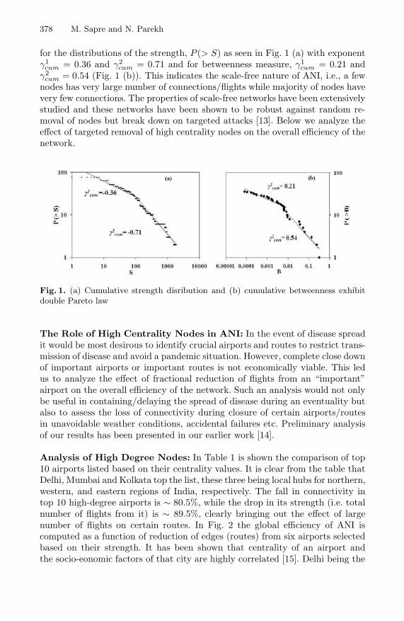
378 M. Sapre and N. Parekh
for the distributions of the strength, P (> S) as seen in Fig. 1 (a) with exponentγ1
cum = 0.36 and γ2cum = 0.71 and for betweenness measure, γ1
cum = 0.21 andγ2
cum = 0.54 (Fig. 1 (b)). This indicates the scale-free nature of ANI, i.e., a fewnodes has very large number of connections/flights while majority of nodes havevery few connections. The properties of scale-free networks have been extensivelystudied and these networks have been shown to be robust against random re-moval of nodes but break down on targeted attacks [13]. Below we analyze theeffect of targeted removal of high centrality nodes on the overall efficiency of thenetwork.
Fig. 1. (a) Cumulative strength disribution and (b) cumulative betweenness exhibitdouble Pareto law
The Role of High Centrality Nodes in ANI: In the event of disease spreadit would be most desirous to identify crucial airports and routes to restrict trans-mission of disease and avoid a pandemic situation. However, complete close downof important airports or important routes is not economically viable. This ledus to analyze the effect of fractional reduction of flights from an “important”airport on the overall efficiency of the network. Such an analysis would not onlybe useful in containing/delaying the spread of disease during an eventuality butalso to assess the loss of connectivity during closure of certain airports/routesin unavoidable weather conditions, accidental failures etc. Preliminary analysisof our results has been presented in our earlier work [14].
Analysis of High Degree Nodes: In Table 1 is shown the comparison of top10 airports listed based on their centrality values. It is clear from the table thatDelhi, Mumbai and Kolkata top the list, these three being local hubs for northern,western, and eastern regions of India, respectively. The fall in connectivity intop 10 high-degree airports is ∼ 80.5%, while the drop in its strength (i.e. totalnumber of flights from it) is ∼ 89.5%, clearly bringing out the effect of largenumber of flights on certain routes. In Fig. 2 the global efficiency of ANI iscomputed as a function of reduction of edges (routes) from six airports selectedbased on their strength. It has been shown that centrality of an airport andthe socio-eonomic factors of that city are highly correlated [15]. Delhi being the
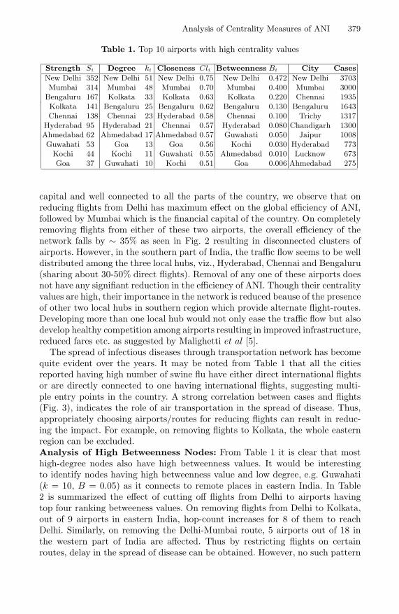
Analysis of Centrality Measures of ANI 379
Table 1. Top 10 airports with high centrality values
Strength Si Degree ki Closeness Cli Betweenness Bi City Cases
New Delhi 352 New Delhi 51 New Delhi 0.75 New Delhi 0.472 New Delhi 3703Mumbai 314 Mumbai 48 Mumbai 0.70 Mumbai 0.400 Mumbai 3000Bengaluru 167 Kolkata 33 Kolkata 0.63 Kolkata 0.220 Chennai 1935Kolkata 141 Bengaluru 25 Bengaluru 0.62 Bengaluru 0.130 Bengaluru 1643Chennai 138 Chennai 23 Hyderabad 0.58 Chennai 0.100 Trichy 1317
Hyderabad 95 Hyderabad 21 Chennai 0.57 Hyderabad 0.080 Chandigarh 1300Ahmedabad 62 Ahmedabad 17 Ahmedabad 0.57 Guwahati 0.050 Jaipur 1008Guwahati 53 Goa 13 Goa 0.56 Kochi 0.030 Hyderabad 773Kochi 44 Kochi 11 Guwahati 0.55 Ahmedabad 0.010 Lucknow 673Goa 37 Guwahati 10 Kochi 0.51 Goa 0.006 Ahmedabad 275
capital and well connected to all the parts of the country, we observe that onreducing flights from Delhi has maximum effect on the global efficiency of ANI,followed by Mumbai which is the financial capital of the country. On completelyremoving flights from either of these two airports, the overall efficiency of thenetwork falls by ∼ 35% as seen in Fig. 2 resulting in disconnected clusters ofairports. However, in the southern part of India, the traffic flow seems to be welldistributed among the three local hubs, viz., Hyderabad, Chennai and Bengaluru(sharing about 30-50% direct flights). Removal of any one of these airports doesnot have any signifiant reduction in the efficiency of ANI. Though their centralityvalues are high, their importance in the network is reduced beause of the presenceof other two local hubs in southern region which provide alternate flight-routes.Developing more than one local hub would not only ease the traffic flow but alsodevelop healthy competition among airports resulting in improved infrastructure,reduced fares etc. as suggested by Malighetti et al [5].
The spread of infectious diseases through transportation network has becomequite evident over the years. It may be noted from Table 1 that all the citiesreported having high number of swine flu have either direct international flightsor are directly connected to one having international flights, suggesting multi-ple entry points in the country. A strong correlation between cases and flights(Fig. 3), indicates the role of air transportation in the spread of disease. Thus,appropriately choosing airports/routes for reducing flights can result in reduc-ing the impact. For example, on removing flights to Kolkata, the whole easternregion can be excluded.Analysis of High Betweenness Nodes: From Table 1 it is clear that mosthigh-degree nodes also have high betweenness values. It would be interestingto identify nodes having high betweenness value and low degree, e.g. Guwahati(k = 10, B = 0.05) as it connects to remote places in eastern India. In Table2 is summarized the effect of cutting off flights from Delhi to airports havingtop four ranking betweeness values. On removing flights from Delhi to Kolkata,out of 9 airports in eastern India, hop-count increases for 8 of them to reachDelhi. Similarly, on removing the Delhi-Mumbai route, 5 airports out of 18 inthe western part of India are affected. Thus by restricting flights on certainroutes, delay in the spread of disease can be obtained. However, no such pattern

380 M. Sapre and N. Parekh
Fig. 2. The impact on Eglobal of ANI asa function of reduction of flights-routesfrom six major hubs in ANI: Delhi,Mumbai, Bengaluru, Kolkata, Chennaiand Hyderabad.
Fig. 3. Correlation between no. offlights from Delhi and no. of reportedswine-flu cases (obtained from Ministryof Health of India [16]), r = 0.84
is observed in the case of removing flights from Delhi to either Hyderabad,Chennai, or Bengaluru. If similar local hubs are developed in western/northernregions, connectivity can be improved which would also help in the economicdevelopment of those regions.Analysis of High Closeness Nodes: The closeness values indicate the accessi-bility of an airport to any other airport in the country. For ANI we observe thatmajority of airports have average closeness value (∼ 0.45), suggesting a goodinter-connectivity between cities. This measure can have important implicationin developing tourism to hill stations (e.g., Kullu Manali, Darjeeling), wild-lifesanctuaries (e.g., Corbett National Park.), historical places (e.g., Agra, Hampi)and religious places (e.g., Puri, Tirupati) apart from improving connectivity tomajor industrial cities (e.g., Jamshedpur). These airports, in general, do not havehigh-degree or high-betweenness values and in some cases are not connected byair. Their closeness values can be increased by connecting them to the nearestlocal hubs. Our analysis of closeness values of various tourist spots show thatthe most popular tourist spot, Goa (0.55), indeed has high closeness value buthill-stations, e.g., Kullu-Manali (0.37) or Agatti Island (0.33) do not, suggestingthe improvement of their connectivity to improve revenue through tourism.
Table 2. The increased “hops” for airports when flights from Delhi to four high-betweenness airports are cut-off is shown.(No. given in bracket)
Kolkata Silchar(3) Tezpur (3) Jorhat(3) Aizwal(2) Dimapur(2)Lilabari(2) Shillong(2) Gaya(2)
Mumbai Latur(3) Solapur(3) Kandla(3) Bhavnagar(2) Nasik(2)
Chennai Madurai(2) Trichy (1)
Bengaluru Agatti(3) Mangaluru(2)

Analysis of Centrality Measures of ANI 381
4 Conclusion
Graph theoretic analysis of weighted ANI helps in identifying “critical” nodes,not necessarily the ones with high connections but also the ones lying on hightraffic-routes (high betweenness) or geographically well distant nodes (high close-ness). Analysis of these high-centrality nodes can help in improving efficiency ofANI, tourism in the country and containing the spread of disease.
References
1. Li, W., Chai, X.: Statistical analysis of airport network of China. Phys. Rev.E. 69,46106 (2004)
2. Guida, M., Funaro, M.: Topology of Italian airport network. Chaos Solitons andFractals 31, 527–536 (2007)
3. Bagler, G.: Analysis of airport network of India as a complex weighted network.Physica A 387, 2972–2980 (2008)
4. Guimera, R., Mossa, S., Turtschi, A., Amaral, L.A.N.: The worldwide air trans-portation network: Anomalous centrality, community structure and cities’ globalroles. PNAS 2, 7794–7799 (2005)
5. Malighetti, G., Martini, G., Paleari, S., Redondi, R.: The Impacts of Airport Cen-trality in the EU Network and Inter-Airport Competition on Airport Efficiency.MPRA (2009)
6. Berger, A., Muller-Hannemann, M., Rechner, S., Zock, A.: Efficient computation oftime-dependent centralities in air transportation networks. In: Katoh, N., Kumar,A. (eds.) WALCOM 2011. LNCS, vol. 6552, pp. 77–88. Springer, Heidelberg (2011)
7. http://www.icao.int
8. The data from the sites of major airlines (2010)9. Barrat, A., Barthelemy, M., Pastor-Satorras, R., Vespignani, A.: The architecture
of complex weighted network. Proc. Natl. Acad. Sci (USA) 101(11), 3747–3752(2004)
10. Latora, V., Marchiori, M.: Efficient Behavior of Small World Networks. Phys. Rev.Lett. 87, 198701 (2001)
11. Newman, M.E.J.: The structure of scientific collaboration network. Proc. Natl.Aca. Sci. 98, 404–409 (2001)
12. Watts, D.J., Strogatz, S.H.: Collective dynamics of ’small-world’ networks. Na-ture 393, 440–442 (1998)
13. Barabasi, A.-L., Albert, R.: Emergence of scaling in random networks. Science 286,509–512 (1999)
14. Sapre, M., Parekh, N.: Analysis of Airport Network of India. In: Poster presentationat Grace Hopper Coneference in Computer Science, Bangalore (2010)
15. Wang, J., Mo, H., Wang, F., Jin, F.: Exploring the network struture and nodalcentrality of China’s air transport network: A complex network approach. Journalof Transport Geography (in press) (2010)
16. http://www.mohfw.nic.in/
Clusters of Multivariate Stationary Time Series
by Differential Evolution and AutoregressiveDistance
Roberto Baragona
Sapienza University of Rome, Dept. of Communication and Social ResearchVia Salaria 113, Rome, Italy
http://w3.uniroma1.it/statstsmeh
Abstract. Clustering MTS is a difficult task that has to be performedin several application fields. We propose a method based on the coeffi-cients of vector autoregressive (VAR) models and differential evolution(DE) that may be applied to sets of stationary MTS. Results from asimulation experiment that includes both linear and non linear MTSare displayed for comparison with genetic algorithms (GAs), principalcomponent analysis (PCA) and the k-means algorithm. Part of the Aus-tralian Sign Language (Auslan) data are examined to show the compar-ative performance of our procedure on a real world data set.
Keywords: Autoregressive distance, Cluster analysis, Differentialevolution, Multivariate time series.
1 Introduction
MTS are of chief interest in a large set of application fields, e.g. econometrics,environmental sciences, seismology, medicine, data mining, speech recognition,video image analysis. Surveys are for example [7] and [8,9]. Often data are col-lected by automatic devices (sensors, electronic transaction documents, the In-ternet) and a large amount of information is available. The standard organizationfor MTS is a rectangular array with m rows (series components, variables, loca-tions) and n columns (observations taken at regular time intervals). Clusteringis a common device which is used to reduce a large set of MTS to a smaller setof MTS representative of homogeneous groups. We assume that data are unla-beled, so that we have to check the existence and find the groups using only theavailable data. We examine in this paper the features that may be computedfrom the popular VAR model estimated matrices of coefficients. We observe formotivating such a choice that such features are simple and effective for cluster-ing stationary MTS and may be easily and quickly computed by least squares.Many other features have been suggested. PCA of similarity matrices has beenproposed for developing procedures for MTS classification [17,14,1]. Extensionsof spectral measures for MTS have been discussed by [5]. The approach intro-duced by [9] splits the clustering procedure into two steps. In the first step each
S.O. Kuznetsov et al. (Eds.): PReMI 2011, LNCS 6744, pp. 382–387, 2011.c© Springer-Verlag Berlin Heidelberg 2011

Clusters of Time Series by Differential Evolution 383
MTS is converted into a sequence of discrete values. In the second step either thedynamic time warping or a symmetric version of the Kullback-Leibler distanceis computed from the discrete data. Many algorithms are available to clustera set of features, in general a set of unlabeled data (see, e.g., [6]). Most effi-cient specially for complicated large data set have been found the meta heuristicmethods (see, e.g., [16]) which solve the clustering problems put in terms of anoptimization problems with respect to some cluster internal validity index (see,e.g., [3,11]). In particular the most used meta heuristic for clustering maybe arethe GAs often in the presence of multiple objective functions (see, e.g., [2]). How-ever DE ([15]) seems more suited to deal with real valued potential solutions,and we suggest using this method for clustering MTS. The paper is organized asfollows. In Sect. 2 the features that we use for clustering are introduced. The DEmethod is illustrated in Sect. 3. In Sect. 4 a simulation study is reported thatsupport the use of the AR weights and DE for clustering MTS. An applicationto a well-known set of real world data is presented in Sect. 5. Sect. 6 concludes.
2 The Autoregressive Weights for Multivariate TimeSeries
Let xt = (x1,t, x2,t, . . . , xm,t)′, where t is a discrete valued time index, be a realvalued m-dimensional MTS which admits the VAR infinite representation
xt =∞∑
i=1
Πixt−i + at, (1)
where the Πi are m×m matrices of coefficients and at is a m-dimensional whitenoise with zero mean and variance covariance matrix Σa. Examples of suchMTS are the popular finite order stationary VAR, the invertible vector moving-average (VMA) and the finite order stationary and invertible vector AR andMA (VARMA) models. Given a MTS data set x1, x2, . . . , xn a finite order LVAR may be fitted to xt with L large enough to obtain a good approximation ofEqn. (1). [10] suggested a test of hypothesis for every pair of MTS in a given setbased on the VAR parameter coefficient matrices estimates Πi, i = 1, . . . , L. Letπi be the column vector obtained by stacking the columns of Πi, i = 1, . . . , L.A set of measurements that may be used to characterize the MTS is the vectorπ = (π′
1, π′2, . . . , π
′L)′. These measurements may be viewed as an extension to
the multivariate framework of the AR distance index introduced by [12] forunivariate time series. We call these measurements as the features of interestthat may capture the characteristic behavior of each MTS in a given set. Adistance measure, e.g. the Euclidean metric, between two feature vectors maybe assumed as the distance between the respective MTS.
3 Differential Evolution Based Clustering
Most clustering algorithms which include centers evolution use GAs. The contri-bution of the present paper aims at showing that DE is a better choice than GAs

384 R. Baragona
if, as it is the case with the AR distance here, chromosomes with real valuedgenes are employed. DE is a population based method that evolves a popula-tion of potential solutions through a sequence of generations. Each solution isa vector x = (x1, x2, . . . , xm)′ ∈ Rm which at each generation undergoes theDE process. A vector v0 (called the base vector) different from x is selectedrandomly in the population. Then two other vectors v1 and v2 are randomlyselected and their difference is scaled by the scale factor F ∈ (0, 1). A new po-tential solution u called mutant is computed u = v0 +F (v1−v2) and recombinedwith the initial individual vector x to produce an offspring vector y by meansof uniform crossover. This means that each element of y is assumed equal tothe corresponding element of the mutant u with a fixed probability pc or equalto the original element of the vector x with probability (1 − pc). Finally y re-places x in the population if a better value of the objective function is obtained.Basically the population size remains the same during the whole DE process.More details and variants may be found in [13]. For implementing the examplesin the following Sect. 4 and 5 we used the Matlab code from [13] modified forthe purpose of clustering MTS. The population consists in a set of vectors withlength g × m2L, where g is the number of cluster and m2L the total number ofthe VAR coefficients. Each vector encodes a sequence of g centers that representclusters of the sequences of AR weights computed from the MTS data set. Weimplemented the fuzzy clustering method with objective function the FCM in-dex Jm for which GAs have been proposed ([3]). The centers evolution includesthe update that takes place in the FCM algorithm as soon as the new clustershave been defined and produces an improvement of the rate of convergence tothe optimal solution. The same device has been included in the GAs clusteringthat we use for performance comparison.
4 Experiments on Artificial Data Sets
In the following simulation experiments the AR weights are computed by fittinga VAR(L) to each artificial MTS in a given set. Then we compare the procedurebased on DE, GAs, PCA and the k-means algorithm. Comparison is made interms of the misclassification error rate (MSCR) and the modified Rand index(MRI) ([4]). As a first experiment, a set of 2-dimensional artificial time seriesdata of length 100 has been generated as in [9] from the bivariate VARMAmodels
xt − μ = Φ(xt−1 − μ) + at − Θat−1, (2)
where μ = (10, 20)′,
Φ =(
1.2 −0.50.6 0.3
), Θ =
(−0.6 0.30.3 0.6
),
and at is a sequence of independent identically normally distributed vectorrandom variables with mean zero and variance covariance matrix
Σ =(
1.0 0.50.5 1.25
).
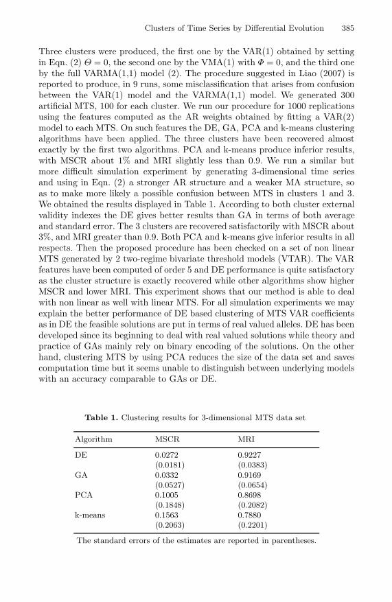
Clusters of Time Series by Differential Evolution 385
Three clusters were produced, the first one by the VAR(1) obtained by settingin Eqn. (2) Θ = 0, the second one by the VMA(1) with Φ = 0, and the third oneby the full VARMA(1,1) model (2). The procedure suggested in Liao (2007) isreported to produce, in 9 runs, some misclassification that arises from confusionbetween the VAR(1) model and the VARMA(1,1) model. We generated 300artificial MTS, 100 for each cluster. We run our procedure for 1000 replicationsusing the features computed as the AR weights obtained by fitting a VAR(2)model to each MTS. On such features the DE, GA, PCA and k-means clusteringalgorithms have been applied. The three clusters have been recovered almostexactly by the first two algorithms. PCA and k-means produce inferior results,with MSCR about 1% and MRI slightly less than 0.9. We run a similar butmore difficult simulation experiment by generating 3-dimensional time seriesand using in Eqn. (2) a stronger AR structure and a weaker MA structure, soas to make more likely a possible confusion between MTS in clusters 1 and 3.We obtained the results displayed in Table 1. According to both cluster externalvalidity indexes the DE gives better results than GA in terms of both averageand standard error. The 3 clusters are recovered satisfactorily with MSCR about3%, and MRI greater than 0.9. Both PCA and k-means give inferior results in allrespects. Then the proposed procedure has been checked on a set of non linearMTS generated by 2 two-regime bivariate threshold models (VTAR). The VARfeatures have been computed of order 5 and DE performance is quite satisfactoryas the cluster structure is exactly recovered while other algorithms show higherMSCR and lower MRI. This experiment shows that our method is able to dealwith non linear as well with linear MTS. For all simulation experiments we mayexplain the better performance of DE based clustering of MTS VAR coefficientsas in DE the feasible solutions are put in terms of real valued alleles. DE has beendeveloped since its beginning to deal with real valued solutions while theory andpractice of GAs mainly rely on binary encoding of the solutions. On the otherhand, clustering MTS by using PCA reduces the size of the data set and savescomputation time but it seems unable to distinguish between underlying modelswith an accuracy comparable to GAs or DE.
Table 1. Clustering results for 3-dimensional MTS data set
Algorithm MSCR MRI
DE 0.0272 0.9227(0.0181) (0.0383)
GA 0.0332 0.9169(0.0527) (0.0654)
PCA 0.1005 0.8698(0.1848) (0.2082)
k-means 0.1563 0.7880(0.2063) (0.2201)
The standard errors of the estimates are reported in parentheses.

386 R. Baragona
5 The Australian Sign Language Data
This data consists of sample of Auslan signs. 27 examples of each of 95 Auslansigns were captured from a native signer using high-quality position trackers.Each vector time series has 15 components series while the length varies from45 to 60 data points. The data have been downloaded from the UCI MachineLearning Repository (http://archive.ics.uci.edu/ml). As in [9] only 5 samples ofeach of the words ’alive’, ’all’, ’boy’, ’cold’ from the directory ’john4’ have beenused for illustration purpose and only the first 11 numeric variables are used.However we considered only the variables 1-4 to avoid singularity of the variancecovariance matrices, as variables 5 and 6 have constant values equal to −1 andvariables 7− 11 have values that are very similar each other. The DE, GA, PCAand k-means algorithms have been applied on the feature set which included theVAR weights computed as the estimates of the matrix coefficients of a VAR(2)model fitted to each one of the 20 4-dimensional MTS. On Table 2 results areevaluated according to the MSCR and the MRI. DE outperforms the remainingalgorithms. The word ’cold’ is correctly recovered by both DE and GA for all the5 samples. The words ’alive’ and ’all’ are recognized for 4 out of 5 samples andthe word ’boy’ for 3 out of 5 samples by DE. The GA, on the other hand, displayssome confusion between the words ’alive’ and ’boy’. The procedure suggested by[9] too makes a specific error in mistaking one of the ’boy’ signs as an ’all’ sign.
Table 2. Clustering algorithms applied to 20 samples from the Auslan data set
Algorithm MSCR MRI
DE 0.2000 0.5136GA 0.4500 0.2344PCA 0.5000 0.2073k-means 0.5500 0.1979
6 Conclusions
A method based on AR distance and DE has been proposed for clustering sta-tionary MTS. Results from a simulation experiment seem quite satisfactory incomparison with GAs and PCA based clustering and the k-means algorithm andsupport the use of our procedure for clustering linear and non linear MTS. Theexecution time for a set of 300 MTS with 100 observations each is on the average0.359 sec for feature extraction while, for the clustering procedure, 1.578 sec forDE, 3.094 sec for GA, 0.871 sec for PCA and 0.015 sec for k-means. So DEseems to attain a fair trade-off between speed and performance. An applicationto some data from the Auslan data set confirms the better performance of ourprocedure with respect to competing alternatives.

Clusters of Time Series by Differential Evolution 387
Acknowledgments. Researchfinancially supportedby ’Ministerodell’Istruzione,Universita e Ricerca Scientifica’, Italy, through grant ’Progetto di InteresseNazionale 2007’ PRIN2007.
References
1. Allefeld, C., Bialonski, S.: Detecting syncronization clusters in multivariatetime series via coarse-graining of Markov chains. Tech. rep., arXiv:0707.2479v1[physics.data-an] (July 17, 2007)
2. Bandyopadhyay, S., Baragona, R., Maulik, U.: Clustering multivariate time seriesby genetic multiobjective optimization. Metron 68, 161–183 (2010)
3. Bezdek, J.C., Pal, N.R.: Some new indexes of cluster validity. IEEE T. Sist. ManCyb. – Part B: Cybernetics 28, 301–315 (1998)
4. Hubert, L., Arabie, P.: Comparing partitions. J. Classif. 2, 193–218 (1985)5. Kakizawa, Y., Shumway, R.H., Taniguchi, M.: Discrimination and clustering for
multivariate time series. J. Am. Stat. Assoc. 93, 328–340 (1998)6. Kaufman, L., Rousseeuw, P.J.: Finding Groups in Data. Wiley, New York (2005)7. Keogh, E., Kasetty, S.: On the need for time series data mining benchmarks: A
survey and empirical demonstration. Data Min. Knowl. Disc. 7, 349–371 (2003)8. Liao, T.W.: Clustering of time series data - a survey. Pattern Recogn. 38, 1857–1874
(2005)9. Liao, T.W.: A clustering procedure for exploratory mining of vector time series.
Pattern Recogn. 40, 2550–2562 (2007)10. Maharaj, E.A.: Comparison and classification of stationary multivariate time series.
Pattern Recogn. 32, 1129–1138 (1999)11. Pakhira, M.K., Bandyopadhyay, S., Maulik, U.: Validity index for crisp and fuzzy
clusters. Pattern Recogn. 37, 487–501 (2004)12. Piccolo, D.: A distance measure for classifying ARIMA models. J. Time Ser.
Anal. 11, 153–164 (1990)13. Price, K.V., Storn, R., Lampinen, J.: Differential evolution, a practical approach
to global optimization. Springer, Berlin (2005)14. Singhal, A., Seborg, D.E.: Clustering multivariate time-series data. J.
Chemometr. 19, 427–438 (2005)15. Storn, R., Price, K.: Differential evolution - a simple and efficient heuristic for
global optimization over continuous spaces. J. Global Optim. 11, 341–359 (1997)16. Winker, P.: Optimization heuristics in econometrics: applications of threshold ac-
cepting. Wiley, Chichester (2001)17. Yang, K., Shahabi, C.: A PCA-based similarity measure for multivariate time se-
ries. In: MMDB 2004: Proceedings of the 2nd ACM international workshop onMultimedia databases, pp. 65–74. ACM, New York (2004)
Neuro-fuzzy Methodology for Selecting Genes
Mediating Lung Cancer
Rajat K. De1 and Anupam Ghosh2
1 Department of Machine Intelligence Unit,Indian Statistical Institute, Kolkata, India
[email protected] Department of Computer Science and Engineering,Netaji Subhash Engineering College, Kolkata, India
Abstract. In this article, we describe neuro-fuzzy models under super-vised and unsupervised learning for selecting a few possible genes medi-ating a disease. The methodology involves grouping of genes based oncorrelation coefficient using microarray gene expression patterns. Themost important group is selected using existing neuro-fuzzy systems[1,2,3,4,5]. Finally, a few possible genes are selected from the most impor-tant group using the aforesaid neuro-fuzzy systems. The effectiveness ofthe methodology has been demonstrated on lung cancer gene expressiondata sets. The superiority of the methodology has been established withfour existing gene selection methods like SAM, SNR, NA and BR. Theenrichment of each gene ontology category of the resulting genes was cal-culated by its P -value. The genes output the low P -value, and indicatethat they are biologically significant. According to the methodology, wehave found more true positive genes than the other existing algorithms.
1 Introduction
Gene selection refers to the task of selecting some informative genes. The goalof gene selection algorithms is to filter out a small set of informative genes thatbest explains experimental variations. It is much cheaper to focus on a smallnumber of informative genes, from the whole genome, that can differentiallyexpress in various diseases. Therefore, using effective gene selection methods,a small list of highly informative genes can be discovered from whole gene set[6], which have direct/indirect role in causing diseases. Thus, these genes can beutilized to construct the classifier for discriminating disease patterns. From datamining point of view, the task of gene selection can be viewed as that of featureselection that is widely used in data preprocessing stage [7,8]. However, geneselection, unlike feature selection in the area of machine learning literature, ischaracterized by the great difference between a huge number of genes and verysmall number of samples.
Several attempts have been made during the past several years for develop-ing methodologies or using feature selection algorithms that select informative
S.O. Kuznetsov et al. (Eds.): PReMI 2011, LNCS 6744, pp. 388–393, 2011.c© Springer-Verlag Berlin Heidelberg 2011

Neuro-fuzzy Methodology for Selecting Genes Mediating Lung Cancer 389
genes from microarray gene expression data. These genes improve the efficiencyof the system in terms of disease prediction accuracy. The attempts include Noisesampling method [9], Bayesian regularization model (BR) [10,11], SignificanceAnalysis of Microarray (SAM) [12], Signal-to-Noise Ratio (SNR) [13], Neighbor-hood analysis (NA) [9]. Most of the above methods are claimed to be capable ofextracting a set of highly informative genes [6].
The present article is an attempt in this regard and provides neuro-fuzzymethodology for gene selection. The methodology involves grouping of genesusing correlation coefficient, followed by selecting the most important groupusing the neuro-fuzzy models. Then the most informative genes are selectedusing neuro-fuzzy methods again. It is to be mentioned here that neuro-fuzzymethods have been developed in [1,2,3,4,5] for the purposed of feature selection.Neuro-fuzzy methodologies are applicable in data rich environment, i.e., if thenumber of samples is quite large compared to the number of features. However,in the present problem, the number of microarray measurements (samples) isquite low compared to the number of genes (features). In order to tackle thissituation, we have proposed a way of generating more data so that neuro-fuzzysystems can be effectively used.
Incorporation of fuzzy set theory enables one to deal with uncertainties in dif-ferent tasks of a pattern recognition system, arising from deficiency (e.g., vague-ness,incompleteness, etc.) in information, in an efficient manner. Artificial NeuralNetworks, having the capability of fault tolerance, adaptivity, and generalization,and scope for massive parallelism, are widely used in dealing with learning andoptimization tasks. In the area of pattern recognition, neuro-fuzzy approacheshave been attempted mostly for designing classification/clustering/feature se-lection or extraction methodologies; the problem of gene selection has not beenaddressed.
The effectiveness of the proposed methodology, along with its superior per-formance over several of other methods, is demonstrated using one microarraygene expression data set dealing with human lung. The performance comparisonis made using t-test and P -value (in terms of the number of enriched attributes).
2 Methodology
Here we describe the proposed methodology for gene selection. The task of geneselection has been considered as the task of feature selection in pattern recogni-tion literature. Since the number of genes is very large compared to the numberof measurements (samples), we have grouped the genes based on the correla-tion coefficient. Then the groups are evaluated using neuro-fuzzy systems undersupervised (NFS) [2,3,4,5] and unsupervised (NFU) [1,3,4,5] learning, and themost important group is selected. Finally, important genes are selected from themost important group using NFS and NFU. For details of NFS and NFU, onemay refer to [1,2,3,4,5].
Let us consider a set X = (x1,x2, . . . ,xn) of n genes for each of which pexpression values in normal samples and q expression values in diseased samples
390 R.K. De and A. Ghosh
are given. We now compute the correlation coefficient among these genes basedon their expression values in normal samples. Thus the correlation coefficient rij
between ith and jth genes is given by
rij =∑p
k=1(xik− mi) × (xjk
− mj)(∑p
i=1(xik− mi)2)1/2 × (
∑pi=1(xjk
− mj)2)1/2(1)
Here mi and mj are the mean of expression values of ith and jth genes, re-spectively, over normal samples. The term xik
denotes kth expression value ofith gene. The correlation coefficient assumes values in the interval [−1, 1]. Whenrij = −1 (+1), there is a strong negative (positive) correlation between ith andjth genes. Genes with high positive correlation are placed into the same group.The main idea of grouping is as follows. If a gene is strongly correlated withanother gene, then the expression value of one of them is linearly dependent onthat of the other. In that case, we may consider one of them as a representativegene and ignore the other.
We now find out the groups of genes in such a way that the genes in thesame groups are strongly correlated. In order to do this, we have computed rij
(Equation (1)) for each pair of genes. If rij ≥ 0.75, then we place these genes inthe same group. In this way, the first group of genes is created. Then we continuein the same way on the remaining genes, and the second group is created. Weproceed in this way till all the genes are placed in one of the groups. Note thatsome singleton groups may also be formed by this process. Thus we have afew groups containing the genes. This process reduces the number of genes andhence reduces the curse of dimensionality. It is to be mentioned here that onemay choose other high value (< 1) instead of 0.75 as the threshold.
We now use NFS or NFU [1,2,3,4,5], in the next step, for selecting the mostimportant group. Since the number of measurements (samples) is quite low, weneed to generate more data. This will be helpful to create a data rich environmentwhere artificial neural networks are more effective. We proceed as follows.
After grouping, let us assume that we have K groups, viz., G1, G2, . . . , Gk, . . . ,GK such that |Gk | = nk, ∀k. Let us also assume that a member of Gk isrepresented by gk = [gk1, gk2, . . . , gkl, . . . , gkp]T such that and gk = xj , forsome value of j. Then we choose one gene for each group and form a vectorv = [v1, v2, . . . , vk, . . . , vK ]T , where vk = gkl, lth sample value. That is, the com-ponents of vector v is the lth normal sample value of K genes that are drawnfrom each group Gk. Similarly, other vs are formed by the other normal samplevalues and we have a total of p such vectors for each draw of K genes, one fromeach group. We thus create a set S of all such vectors from normal samples v sothat the numbers of such vectors in S is
s = |S| = p ×K∏
k=1
nk (2)

Neuro-fuzzy Methodology for Selecting Genes Mediating Lung Cancer 391
Similarly, another set S′ of vectors v′ is created from the diseased samplessuch that
s′ = |S′| = q ×K∏
k=1
nk (3)
Now we have two sets, S and S′ of vectors v and v′ respectively. For NFS, weconsider that normal and diseased samples form two classes, viz., normal anddiseased. We take the number of input nodes as K, and the other nodes alongwhich the architecture of the system is decided automatically [2,3,4,5]. In thecase of NFU, the number of input nodes is 2K, and the other nodes along whichits architecture is decided automatically [1,3,4,5]. The first K nodes receive thevectors v as their inputs and second K nodes receive v′. Thus the number ofsuch presentations is s × s′. After learning in both the systems, we get weightvalues representing importance of each group. Thus the most important groupis selected for which the weight value is the highest.
Once the most important group is selected, only the genes in this group areconsidered. If the number of genes in the most important group is N (N <<n), the numbers of input nodes in NFS and NFU are N and 2N , respectively.The remaining parts of the architecture of both the systems are determinedautomatically. As in the case of selection of groups, the number of classes forNFS is 2. For NFU, the first N input nodes receive expression values of genes(in the most important group) of normal samples and the next N nodes receivethat of diseased samples. Thus the number of presentations in NFU is p × q.After learning, we get weight values corresponding to each gene representingits importance. Then we select a few important genes based on the connectionweights of NFS or NFU.
3 Results
In this section, the effectiveness of the proposed methodology is demonstratedon human lung expression data [14]. A comparative analysis with SAM, SNR,BR, NA is also included.
We have found 6 groups, containing 1659, 1247, 1290, 741, 666, and 1526genes respectively. The group containing 1659 genes has been selected as the mostimportant group by both NFS and NFU. Applying NFS and NFU, we have found30 and 32 genes respectively. Among these genes, we have found 22 genes thatare present in both the results. Finally, we have selected 20 most important genesbased on the connection weights of NFS and NFU. These selected genes are thenevaluated for their role in causing lung cancer through computing the numberof functional enrichments. We have performed t-test for the genes identifiedby other gene selection algorithms like SAM, SNR, NA and BR. But highlysignificant (99.9% significance level) genes like PFKP, TYMS, IARS, and HLA-B are not present in the first twenty selected genes by these methods. Thisresult suggests that NFS and NFU are able to find more significant genes thanthe existing methods.

392 R.K. De and A. Ghosh
Table 1. Comparative results on number of attributes of various sets of genes
No. of AttributesDataset Gene set NFS NFU SAM SNR NA BR
Lung First 5 62 80 14 21 26 27expression First 10 75 76 13 9 15 21
Data First 15 80 82 30 14 16 16First 20 82 75 28 13 15 16
In order to validate the results statistically, we have applied t-test on thegenes identified by NFS, NFU, SAM, SNR, NA and BR. Here we have identifiedsome important genes like CALCA (4.02), PFKP (5.78), TYMS (3.98), IGFBP3(6.98), IARS (5.98), HBB (7.08), HLA-B (5.42), SFTPA2 (6.89), and TNF (4.23).The number in the bracket indicates t-value corresponding to the gene. The t-value of these set of genes exceeds the value for p = 0.001. It indicates that theseset of genes are highly significant (99.9% level of significance). Similarly, geneslike IGHG3 (2.67), PRKACA (2.89), SORT1 (2.76), MEN1 (3.15), SFTPA1(2.92) and IGHM (3.25) exceeds the t-value for p = 0.01. This means that thesegenes are significant at the level of 99%. Likewise, RPLP0 (2.12), SMCIL1 (2.07),MGP (2.31), RNASE1 (2.43), SFTPC (2.37), and HLA-DRA (2.27) genes areimportant at the level of 95% significance.
In our study, the enrichment of each GO category [15] for each of the genes hasbeen calculated by its P -value. A low P -value indicates that the genes belong-ing to the enriched functional categories are biologically significant. Here onlyfunctional categories with P −value < 5.0×10⁻⁵ are considered. We have madecomparative study, with other methods, viz., SAM, SNR, NA, BR in terms oftheir ability to identify functionally enriched genes. Table 1 shows the number offunctionally enriched attributes corresponding to these methods for different setsof genes. It is found that NFS and NFU performed the best. These results showthat the proposed methodology has been able to select more important genesresponsible for mediating a disease than the other methods considered here.
4 Conclusions
In this article, we have provided a methodology based on neuro-fuzzy modelsfor the selection of genes whose over/under expression may cause diseases. Themethodology, first of all, finds various groups of genes based on correlation val-ues. This is followed by determining the most important group. The genes in thisgroups are evaluated using NFS and NFU. This results in important genes is me-diating development of a particular disease. The effectiveness of the methodologyis demonstrated on various gene expression data sets where each gene is treatedas a feature. The most important genes obtained by the methodology are alsoverified using their P -values [15]. The superior performance of the methodologycompared to some existing ones have been shown. The results are verified usingt-test, some existing results.

Neuro-fuzzy Methodology for Selecting Genes Mediating Lung Cancer 393
References
1. Pal, S.K., De, R.K., Basak, J.: Unsupervised feature evaluation: A neuro-fuzzyapproach. IEEE Trans. Neural Networks 11, 366–376 (2000)
2. De, R.K., Basak, J., Pal, S.K.: Neuro-fuzzy feature evaluation with theoreticalanalysis. Neural Networks 12, 1429–1455 (1999)
3. Basak, J., De, R.K., Pal, S.K.: Fuzzy feature evaluation index and connectionistrealization-ii: Theoretical analysis. Information Sciences 111, 1–17 (1998)
4. Basak, J., De, R.K., Pal, S.K.: Unsupervised feature selection using neuro-fuzzyapproach. Pattern Recognition Letters 19, 997–1006 (1998)
5. Pal, S.K., Basak, J., De, R.K.: Fuzzy feature evaluation index and connectionistrealization. Information Sciences 105, 173–188 (1998)
6. Bezdek, J., Pal, S.K.: Fuzzy models for pattern recognition. IEEE Press, New York(1992)
7. Kraaijveld, M.A., Mao, J., Jain, A.K.: A nonlinear projection method based on ko-honen topology preserving maps. IEEE Trans. Neural Networks 6, 548–559 (1995)
8. Rubner, J., Tavan, P.: A self-organizing network for principal component analysis.Europhys. Lett 10, 693–698 (1989)
9. Golub, T.R., Slonim, T.K., Tamayo, P., Huard, C., Gaasenbeek, M., Mesirov, J.P.,Coller, H., Downing, J.R., Caliguri, M.A., Bloomeld, C.D., Lander, E.S.: Molecularclassification of cancer: class discovery and class prediction by gene expressionmonitoring. Science 286, 531–537 (1999)
10. Shevade, S.K., Keerthi, S.S.: A simple and efficient algorithm for gene selectionusing sparse logistic regression. Bioinformatics 19, 2246–2253 (2003)
11. Cawley, G.C., Talbot, N.L.C.: Gene selection in cancer classification using sparse lo-gistic regression with bayesian regularization. Bioinformatics 22, 2348–2355 (2006)
12. Goh, L., Song, Q., Kasabov, N.: A novel feature selection method to improveclassification of gene expression data. In: APBC (2004)
13. Tusher, V.G., Tibshirani, R., Chu, G.: Significance analysis of microarrays appliedto the ionizing radiation response. Proc. Natl. Acad. Sci. USA 98 (2001)
14. Beer, G.D., et al.: Gene-expression profilespredict survival of patients with lungadenocarcinoma. Nature Medicine 8, 816–823 (2002)
15. Kim, D.W., Lee, K.H., Lee, D.: Detecting clusters of different geometrical shapesin microarray gene expression data. Bioinformatics 21, 1927–1934 (2005)
A Methodology for Handling a New Kind of
Outliers Present in Gene Expression Patterns
Anindya Bhattacharya1 and Rajat K. De2,
1 Department of Computer Science and Engineering,Netaji Subhash Engineering College, Kolkata 700152, India
2 Machine Intelligence Unit, Indian Statistical Institute, Kolkata 700108, India
Abstract. Performance of clustering algorithms is largely dependenton selected similarity measure. Efficiency in handling outliers is a majorcontributor to the effectiveness of a similarity measure. In the presentwork, we discuss the problem of handling outliers with different existingsimilarity measures, and introduce the concepts of a new kind of out-liers present in gene expression patterns. We formulate a new similarity,incorporated in Euclidean distance and Pearson correlation coefficient,and then use them in various clustering algorithms to group differentgene expression profiles. Assessment of the results are done by usingfunctional annotation. Different existing similarity measures in their tra-ditional form are also used with clustering algorithms for performancecomparisons. The results suggest that the new similarity improves per-formance, in terms of finding biologically relevant groups of genes, of allthe considered clustering algorithms.
1 Introduction
Clustering algorithm involves measuring similarity between a pair of objects.Some standard similarity measures used in various clustering algorithms in-clude Euclidean distance, various correlation coefficients, Mahalanabis distance.Choice of a similarity measure plays an important role in the performance of aclustering algorithm.
If the objects in a dataset are evenly distributed over the space, the aforesaidsimilarity measures would be effective. On the other hand, if some of objects dueto noise or other factors, called outliers, are included in a dataset, these simi-larity measures may not lead to good performance of the clustering algorithms.They may be biased towards these outliers. There exist various methods forhandling such outliers. They include, among others, statistical approach [1]-[3],distance-based approach, clustering-based approach [4]-[6], density-based localoutlier detection approach [7,5] and deviation-based approach [8].
If the expression value(s) of a single (both) gene(s) corresponding to a samplediffer much from its (their) mean expression value(s) of the other samples, thenthe expression value(s) for this(ese) sample(s) differ drastically for the pair of
Corresponding author.
S.O. Kuznetsov et al. (Eds.): PReMI 2011, LNCS 6744, pp. 394–399, 2011.c© Springer-Verlag Berlin Heidelberg 2011
A Methodology for Handling a New Kind of Outliers 395
genes. This gives rise to the notion of a different kind of outlier which is in-troduced here. That is, the sample is an outlier with respect to the gene pair.Distance/similarity measures used by different clustering algorithms are unableto treat an outlier sample and a normal sample differently. All the samples con-tribute equally during the measurement of distance/similarity.
In order to improve performance of the various similarity measures (includingEuclidean distance and Pearson correlation coefficient), with respect to betterability of handling outliers, we introduce the concept of assigning weight values tosamples. Instead of using a sample value for the similarity measure, we multiplya weight value with expression value of a sample and then use the resulting value.Weight values are determined in such a way that possible outliers are assignedsmaller weight values (i.e., nearly equal to zero). Weight values for non outliersare large, and are nearly equal to ‘one’. With this new similarity, Euclideandistance or Pearson correlation coefficient involves low contribution of outliersamples and high contribution of non outlier samples.
In order to incorporate this varying contribution, we assign a weight valueto gene expression samples. Any similarity measure that computes pair wisedistance similarity, can use the weight assignment technique for better han-dling the outliers. For comparison, Euclidean distance with weight (WD) andwithout weight (D), Pearson correlation coefficient with weight (WCorr) andwithout weight (Corr), Spearman rank-order correlation coefficient (RankCorr)and Jackknife correlation coefficient (JackCorr) are used with clustering algo-rithms K-means [9,8,10], DCCA [11] and ACCA [12]. All the instances of thesealgorithms are applied to different gene expression datasets and performancesare assessed.
2 A New Kind of Outlier
Due to error or other factors in microarray measurements, the expression profilesfor a pair of genes may be similar over all the samples except for a few. For thesefew samples, expression values of the same pair of genes may differ drasticallyfrom the other samples. In other words, the expression value(s) of a single (both)gene(s) corresponding to the sample differ much from its (their) mean expressionvalue(s) over the other samples. The sample(s) for which the expression valuesdiffer drastically for the pair of genes, give rise to the notion of a different kindof outlier. That is, the sample is an outlier with respect to the gene pair. Itmay be mentioned here that this outlier is different from the notion of outliersalready available in literature [8]. In the later case, the gene as a whole needsto be treated as an outlier with respect to a group of genes, in contrary to theformer one where a sample is considered as an outlier corresponding to a genepair. This situation affects clustering if we consider similarity computation basedon expression values only. We introduce a novel methodology to take care of theeffect of such outliers.

396 A. Bhattacharya and R.K. De
3 A Methodology for Handling a New Kind of Outliers
Let us consider a set of n genes X = g1, g2, . . . , gn, for each of which m expres-sion values are given. Let us also consider a set of m microarray experiments/samples (measurements) Y = e1, e2, . . . , em. For each experiment, we haven expression values corresponding to n genes in X . That is, for each gene gi,there is an m-dimensional vector xi, where xil is the expression value of gi inlth experiment el. Similarity between gene pair (gi, gj) may be computed usingEuclidean distance D(xi, xj) or Pearson correlation coefficient Corr(xi ,xj), andare defined, respectively, as
D(xi,xj) =
√√√√m∑
l=1
(xil − xjl)2 (1)
and
Corr(xi ,xj) =
m∑
l=1
(xil − xi)(xjl − xj)
√√√√m∑
l=1
(xil − xi)2m∑
l=1
(xjl − xj)2
. (2)
Here xi and xj are mean values over m expression values of ith and jth genesrespectively.
If lth expression values of a co-expressed, co-regulated gene pair (gi, gj), corre-sponding to an experiment el, are such that the sample is an outlier with respectto gene pair (gi, gj), both Equations 1 and 2 may be biased towards this outlier.That is, if we consider Equation 2 for measuring similarity, the value shouldideally be closed to 1 for a pair of co-regulated genes. Due to this outlier, thecorrelation value will differ much from 1. In order to reduce this type of mislead-ing contribution of outlier, we introduce the notion of weighting coefficient wlij
corresponding to lth expression value and gene pair (gi, gj), for all l, i, j.We determine the weight values so as to reduce the effect of such outliers by
assigning lower weight values corresponding to the outlier samples of gene pair(gi, gj) and a higher weight values to the other samples. In other words, higherthe difference in lth expression values of the genes in the pair (gi, gj) from theirmeans, lower is the value of the weight wlij . Considering Euclidean distance forcomputing difference in lth expression values of both the genes gi and gj fromtheir means, we have
Dijl =√
(til − ti)2 + (tjl − tj)2, (3)
where til and tjl are normalized expression values in [0, 1] of xil and xjl
respectively. Similarly, ti and tj are mean of normalized expression values, com-puted over all the samples, of gene gi and gj respectively. Here we have consid-ered normalized expression values in Equation 3, for keeping Dijl bounded to

A Methodology for Handling a New Kind of Outliers 397
√2 (
√(1 − 0)2 + (0 − 1)2 =
√2). For an outlier sample, measured value of Dijl
should be high. Weight value wlij for an outlier sample el corresponding to a pairof gene (gi, gj) should be low. Thus relationship between Dijl and wlij shouldbe such that, increase in Dijl should cause decrease in wlij and vice versa.
In order to reflect such relationship between Dijl and wlij , here we considerexponential function to define weight wlij of a sample el corresponding to a pairof gene (gi, gj). Thus
wlij = e−α×Dijl , (4)
where α ≥ 1 is a constant. Here the value of α should be such that wlij is nearlyequal to zero for Dijl =
√2. On the other hand, wlij should tend to one for a
non-outlier sample. In fact this happens as Dijl tends to zero for a non-outliersample.
Thus the weight function incorporates wlij , for each lth experiment, in Equa-tions 1 and 2. In these Equations, xil and xjl are replaced by x
(w)ijl = wlij × xil
and x(w)jil = wlij × xjl respectively. Similarly, mean values xi and xj , in Equa-
tion 2, are replaced by x(w)ijl = 1
m
∑ml=1 wlij × xil and x
(w)jil = 1
m
∑ml=1 wlij × xjl
respectively. It is to be mentioned here that x(w)ijl = x
(w)jil , although both of them
involved the same wlijs. It is further to be noted that the terms til, tjl, ti and tjin Equation 3 are computed using xil, xjl only. Thus we get distance WD(xi,xj)and correlation coefficient WCorr(xi,xj) between a gene pair (gi, gj), based onEuclidian distance and Pearson correlation coefficient respectively.
Now the problem remains with the estimation of α-value in Equation 4. Thisis determined form a plot of WD or WCorr for different pairs of genes withrespect to α. From this plot, we have chosen α values at which similarity values(WD or WCorr) get saturated.
4 Results
The effectiveness of the weight assignment method along with comparative anal-ysis with the aforesaid similarity measures is demonstrated with K-means [9,8,10],DCCA [11] and ACCA [12] clustering algorithms using five gene expressiondatasets of Yeast. Datasets are described in Table 1. The performance of allthe algorithms is also demonstrated using P -value on functional annotation.
For gene expression data analysis, P -value of GO functional category/attribute represents the probability of observing at least a given number ofgenes, in a cluster, from a specific GO functional category/attribute. A spe-cific GO functional category is said to be “enriched” if the corresponding P -value is less than a predefined threshold value. A low P -value indicates that thegenes belonging to the enriched functional categories are biologically significantin the corresponding clusters. In the present work, only attributes with P -value< 1.0 × 10⁻⁷ are reported as enriched. A clustering solution is considered tobe more reliable if the number of enriched functional attributes obtained froma cluster is high. In order to compare the performance of different clustering
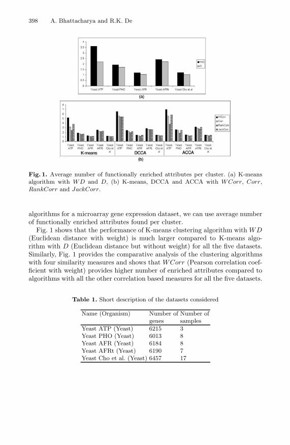
398 A. Bhattacharya and R.K. De
Fig. 1. Average number of functionally enriched attributes per cluster. (a) K-meansalgorithm with WD and D, (b) K-means, DCCA and ACCA with WCorr, Corr,RankCorr and JackCorr.
algorithms for a microarray gene expression dataset, we can use average numberof functionally enriched attributes found per cluster.
Fig. 1 shows that the performance of K-means clustering algorithm with WD(Euclidean distance with weight) is much larger compared to K-means algo-rithm with D (Euclidean distance but without weight) for all the five datasets.Similarly, Fig. 1 provides the comparative analysis of the clustering algorithmswith four similarity measures and shows that WCorr (Pearson correlation coef-ficient with weight) provides higher number of enriched attributes compared toalgorithms with all the other correlation based measures for all the five datasets.
Table 1. Short description of the datasets considered
Name (Organism) Number of Number ofgenes samples
Yeast ATP (Yeast) 6215 3Yeast PHO (Yeast) 6013 8Yeast AFR (Yeast) 6184 8Yeast AFRt (Yeast) 6190 7Yeast Cho et al. (Yeast) 6457 17
A Methodology for Handling a New Kind of Outliers 399
5 Conclusions
Here we have introduced the concepts of a new kind of outlier and a method-ology to handle such outliers. New outliers are the samples with respect to agene pair, for which sample values show large difference from the other samplescorresponding to the gene pair. Incorporation of the notion of weight helps indealing with such outliers while measuring similarity between a pair of gene.
The results suggest that assignment of weight with a similarity measure im-proves the performance of clustering algorithms in obtaining more biologicallysignificant clusters. The main advantage of weight assignment method is that itis able to deal with outliers without deleting them. Weight assignment methoddescribed here is a general framework. Thus it can be used with any distancebased similarity measure without changing the basic formulation of that simi-larity measure.
References
1. Hawkins, D.: Identification of Outliers. Chapman and Hall, London (1980)2. Rousseeuw, P., Leory, A.: Robust Regression and Outlier Detection. Wiley, New
York (1987)3. Barnett, V., Lewis, T.: Outliers in Statistical Data. Wiley, New York (1994)4. Kaufman, L., Rousseeuw, P.J.: Finding Groups in Data: An Introduction to Cluster
Analysis. Wiley, New York (1990)5. Shekhar, S., Chawla, S.: A Tour of Spatial Databases. Prentice-Hall, New Jersey
(2002)6. Hu, T., Sung, S.Y.: Detecting pattern-based outliers. Pattern Recognition Let-
ters 24, 3059–3068 (2003)7. Schiffman, S.S., Reynolds, M.L., Young, F.W.: Introduction to Multidimensional
Scaling: Theory, Methods and Applications. Academic Press, New York (1981)8. Han, J., Kamber, M.: Data Mining: Concepts and Techniques. Morgan Kaufmann,
San Francisco (2001)9. Jain, A.K., Dubes, R.C.: Algorithms for Clustering Data. Prentice-Hall, New Jersey
(1988)10. Tavazoie, S., Hughes, J.D., Campbell, M.J., Cho, R.J., Church, G.M.: Systematic
determination of genetic network architecture. Nature Genetics 22, 281–285 (1999)11. Bhattacharya, A., De, R.K.: Divisive correlation clustering algorithm (DCCA) for
grouping of genes: Detecting varying patterns in expression profiles. Bioinformat-ics 24, 1359–1366 (2008)
12. Bhattacharya, A., De, R.K.: Average correlation clustering algorithm (ACCA) forgrouping of co-regulated genes with similar pattern of variation in their expressionvalues. Journal of Biomedical Informatics 43, 560–568 (2010)

Developmental Trend Derived from Modules of
Wnt Signaling Pathways
Losiana Nayak and Rajat K. De
Machine Intelligence Unit, Indian Statistical Institute203 B. T. Road, Kolkata - 700108, India
losiana t,[email protected]://www.isical.ac.in/~losiana_t,rajat
Abstract. In this paper, we deal with the idea of creating a devel-opmental trend from Wnt signaling pathways of different species. Wntsignaling pathway is involved in many crucial biological processes in-cluding from early embryonic development to stem cell management atlater stages. The pathway varies in topology and size for each speciesthat gets reflected in its modules. A comparison among species-specificpathways, taking into account the modules and pathway structure (interms of nodes and edges) will throw light on crucial turning points inthe development of Wnt signaling pathway. Hence, 31 species-specificWnt signaling pathways have been modularized by the Modularizationalgorithm already developed by the authors. The modules were com-pared among themselves to find the trend of development. The trendestablished conserved modules among these pathways.
Keywords: Modularization algorithm, Evolution, Phylogenetic treeconstruction, Computational Phylogenetics.
1 Introduction
In biological terms, a signal transduction pathway, is a set of established genesand related factors, which operate in synchronous manner to create cascades ofreactions, ultimately generating a response to stimuli in vivo. From graph theo-retical point of view, these genes and related factors can be considered as nodesand the interactions among them as edges of a network. A pathway conceived insuch a way is open to all kind of network analysis paradigms. Network compar-ison (by alignment) to uncover biological functions and phylogeny [1] is one ofthem. Networks derived from biological pathways (gene regulatory, metabolic,signal transduction, protein-protein interaction networks) can be aligned by sizeof the network, sequence similarity of the genes/proteins, functional similarity ofthe enzymes/proteins and presence of common topological structures (graphlets)among others. One or all of these factors are considered while creating a treefrom a set of biological networks. In addition to such factors, we add anotherfactor named ‘modules’ [2]. Modules throw light on operational sophisticationof a network. It is dependent on two other parameters, viz., size (nodes) andtopology (interactions). A tree generated by taking these three linked parame-ters can shed enough light on subtle changes of the network among the species,
S.O. Kuznetsov et al. (Eds.): PReMI 2011, LNCS 6744, pp. 400–405, 2011.c© Springer-Verlag Berlin Heidelberg 2011
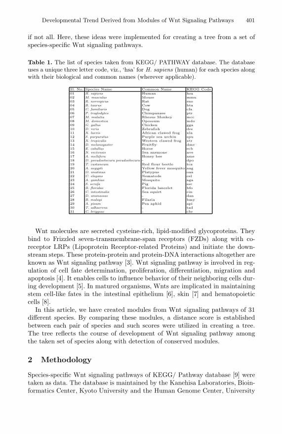
Developmental Trend Derived from Modules of Wnt Signaling Pathways 401
if not all. Here, these ideas were implemented for creating a tree from a set ofspecies-specific Wnt signaling pathways.
Table 1. The list of species taken from KEGG/ PATHWAY database. The databaseuses a unique three letter code, viz., ‘hsa’ for H. sapiens (human) for each species alongwith their biological and common names (wherever applicable).
Sl. No. Species Name Common Name KEGG Code01 H. sapiens Human hsa02 M. musculus Mouse mmu03 R. norvegicus Rat rno04 B. taurus Cow bta05 C. familiaris Dog cfa06 P. troglodytes Chimpanzee ptr07 M. mulatta Rhesus Monkey mcc08 M. domestica Opossum mdo09 G. gallus Chicken gga10 D. rerio Zebrafish dre11 X. laevis African clawed frog xla12 S. purpuratus Purple sea urchin spu13 X. tropicalis Western clawed frog xtr14 D. melanogaster Fruitfly dme15 E. caballus Horse ecb16 N. vectensis Sea anemone nve17 A. mellifera Honey bee ame18 D. pseudoobscura pseudoobscura - dpo19 T. castaneum Red flour beetle tca20 A. aegypti Yellow fever mosquito aag21 O. anatinus Platypus oaa22 C. elegans Nematode cel23 A. gambiae Mosquito aga24 S. scrofa Pig ssc25 B. floridae Florida lancelet bfo26 C. intestinalis Sea squirt cin27 D. ananassae - dan28 B. malayi Filaria bmy29 A. pisum Pea aphid api30 T. adhaerens - tad31 C. briggsae - cbr
Wnt molecules are secreted cysteine-rich, lipid-modified glycoproteins. Theybind to Frizzled seven-transmembrane-span receptors (FZDs) along with co-receptor LRPs (Lipoprotein Receptor-related Proteins) and initiate the down-stream steps. These protein-protein and protein-DNA interactions altogether areknown as Wnt signaling pathway [3]. Wnt signaling pathway is involved in reg-ulation of cell fate determination, proliferation, differentiation, migration andapoptosis [4]. It enables cells to influence behavior of their neighboring cells dur-ing development [5]. In matured organisms, Wnts are implicated in maintainingstem cell-like fates in the intestinal epithelium [6], skin [7] and hematopoieticcells [8].
In this article, we have created modules from Wnt signaling pathways of 31different species. By comparing these modules, a distance score is establishedbetween each pair of species and such scores were utilized in creating a tree.The tree reflects the course of development of Wnt signaling pathway amongthe taken set of species along with detection of conserved modules.
2 Methodology
Species-specific Wnt signaling pathways of KEGG/ Pathway database [9] weretaken as data. The database is maintained by the Kanehisa Laboratories, Bioin-formatics Center, Kyoto University and the Human Genome Center, University
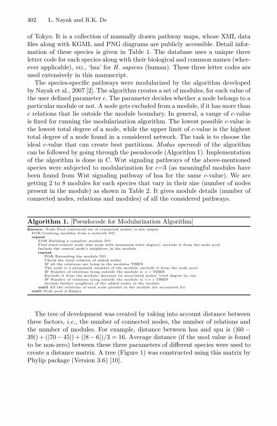
402 L. Nayak and R.K. De
of Tokyo. It is a collection of manually drawn pathway maps, whose XML datafiles along with KGML and PNG diagrams are publicly accessible. Detail infor-mation of these species is given in Table 1. The database uses a unique threeletter code for each species along with their biological and common names (wher-ever applicable), viz., ‘hsa’ for H. sapiens (human). These three letter codes areused extensively in this manuscript.
The species-specific pathways were modularized by the algorithm developedby Nayak et al., 2007 [2]. The algorithm creates a set of modules, for each value ofthe user defined parameter c. The parameter decides whether a node belongs to aparticular module or not. A node gets excluded from a module, if it has more thanc relations that lie outside the module boundary. In general, a range of c-valueis fixed for running the modularization algorithm. The lowest possible c-value isthe lowest total degree of a node, while the upper limit of c-value is the highesttotal degree of a node found in a considered network. The task is to choose theideal c-value that can create best partitions. Modus operandi of the algorithmcan be followed by going through the pseudocode (Algorithm 1). Implementationof the algorithm is done in C. Wnt signaling pathways of the above-mentionedspecies were subjected to modularization for c=3 (as meaningful modules havebeen found from Wnt signaling pathway of hsa for the same c-value). We aregetting 2 to 8 modules for each species that vary in their size (number of nodespresent in the module) as shown in Table 2. It gives module details (number ofconnected nodes, relations and modules) of all the considered pathways.
Algorithm 1. [Pseudocode for Modularization Algorithm]Ensure: Node Pool (universal set of connected nodes) is not empty
FOR Creating modules from a network DOrepeat
FOR Building a complete module DOFind start/central node (the node with maximum total degree); exclude it from the node poolInclude the central node’s neighbors in the modulerepeat
FOR Extending the module DOCheck the total relation of added nodesIF all the relations are lying in the modules THENThe node is a permanent member of the module; exclude it from the node poolIF Number of relations lying outside the module is > c THENExclude it from the module; decrease its associated nodes’ total degree by oneIF Number of relations lying outside the module is <= c THENInclude further neighbors of the added nodes in the module
until All the relations of each node present in the module are accounted foruntil Node pool is Empty
The tree of development was created by taking into account distance betweenthree factors, i.e., the number of connected nodes, the number of relations andthe number of modules. For example, distance between hsa and spu is (|60 −39|)+ (|70− 45|)+ (|8− 6|)/3 = 16. Average distance (if the mod value is foundto be non-zero) between these three parameters of different species were used tocreate a distance matrix. A tree (Figure 1) was constructed using this matrix byPhylip package (Version 3.6) [10].

Developmental Trend Derived from Modules of Wnt Signaling Pathways 403
3 Results and Discussion
In this section, we have compared modules of 31 different species (aag, aga, ame,api, bfo, bmy, bta, cbr, cel, cin, cfa, dan, dme, dpo, dre, ecb, gga, hsa, mcc, mdo,mmu, nve, oaa, ptr, rno, ssc, spu, tad, tca, xla and xtr). Module details are givenin Table 2.
Table 2. Module information of species-specific Wnt signaling pathways. [sp.: threelettered species code, n: number of connected nodes in a species-specific pathway; r:number of relations present the connected component of a species-specific pathway;t: total number of modules created from a species-specific pathway]. The moduleshave been created for c=3. Each module’s size in terms of nodes is given with itin parentheses. The table throws light on the developmental trend of Wnt signalingpathways among the taken set of species.
sp. n r t WNT (DVL)1 Axin β-catenin TCF p53 (DVL)2 PLChsa 60 70 8 WNT [8] (DVL)1 [7] Axin [4] β-catenin [8] TCF [14] p53 [2] (DVL)2 [10] PLC [7]
mmu 60 70 8 WNT [8] (DVL)1 [7] Axin [4] β-catenin [8] TCF [14] p53 [2] (DVL)2 [10] PLC [7]rno 59 69 8 WNT [7] (DVL)1 [7] Axin [4] β-catenin [8] TCF [14] p53 [2] (DVL)2 [10] PLC [7]bta 58 68 8 WNT [7] (DVL)1 [6] Axin [4] β-catenin [8] TCF [14] P53 [2] (DVL)2 [10] PLC [7]cfa 58 68 8 WNT [8] (DVL)1 [7] Axin [4] β-catenin [7] TCF [13] p53 [2] (DVL)2 [10] PLC [7]ptr 58 67 8 WNT [8] (DVL)1 [7] Axin [4] β-catenin [8] TCF [13] p53 [2] (DVL)2[10] PLC [6]mcc 55 63 8 WNT [7] (DVL)1 [6] Axin [4] β-catenin [8] TCF [13] p53 [2] (DVL)2 [8] PLC [7]mdo 54 64 7 WNT [8] (DVL)1 [7] Axin[2] β-catenin [9] TCF [11] - (DVL)2 [10] PLC [7]gga 54 63 8 WNT [7] (DVL)1 [6] Axin [3] β-catenin [8] TCF [11] p53 [2] (DVL)2 [10] PLC [7]dre 52 60 7 WNT [8] - Axin [4] β-catenin [7] TCF [13] p53 [2] (DVL)2 [11] PLC [7]xla 43 45 6 WNT [7] - - β-catenin [8] TCF [11] p53 [2] (DVL)2 [8] PLC [7]spu 39 45 6 - (DVL)1 [7] Axin [2] β-catenin [5] TCF [10] - (DVL)2 [9] PLC [6]xtr 37 36 6 WNT [3] - - β-catenin [7] TCF [6] p53 [2] (DVL)2 [12] PLC [7]dme 36 42 7 WNT [6] (DVL)1 [5] Axin [2] β-catenin [6] TAK1 [2] - (DVL)2 [9] PLC [6]ecb 36 38 7 (Frizzled)1 [5] (DVL)1 [3] - β-catenin [9] TAK1 [2] p53 [2] (DVL)2 [8] PLC [7]nve 32 33 6 (Frizzled)1 [5] - Axin [5] β-catenin [6] TAK1 [2] - (DVL)2 [7] PLC [7]ame 30 32 5 - (DVL)1 [4] - β-catenin [9] TAK1 [2] - (DVL)2 [8] PLC [7]dpo 28 30 4 (Frizzled)1 [8] - - β-catenin [7] - - (DVL)2 [8] PLC [5]tca 26 27 4 (Frizzled)1 [7] - - β-catenin [7] - - (DVL)2 [6] PLC [6]aag 24 22 4 (Frizzled)1 [4] - - β-catenin [4] - - (DVL)2 [10] PLC [6]oaa 22 22 4 WNT [2] - - β-catenin [7] - - (DVL)2 [8] PLC [5]cel 22 20 3 - - - β-catenin [10] - - RhoA [6] PLC [6]aga 20 18 3 (Frizzled)1 [11] - - β-catenin [4] - - - PLC [5]ssc 19 16 4 FRP [2] - - β-catenin [5] TCF [7] - - PLC [5]bfo 18 16 3 - - - β-catenin [9] - - (DVL)2 [5] PLC [4]cin 17 14 3 - (DVL)1 [7] - - - - (DVL)2 [5] PLC [5]dan 16 12 4 - (DVL)1 [2] - β-catenin [4] - - (DVL)2 [5] PLC [5]bmy 13 11 3 - (DVL)1 [4] - - - - (DVL)2 [5] PLC [4]api 13 10 3 - (DVL)1 [4] - - - - (DVL)2 [5] PLC [4]tad 6 4 2 - - - - - - Rac [2] PLC [4]cbr 4 3 1 - (DVL)1 [4] - - - - - -
Comparison of the modules brought forward their functional conservationamong the taken species. Modules Wnt and β − catenin were found to be con-served in 9 species (hsa, mmu, rno, bta, cfa, ptr, mcc, mdo and gga). ModuleTCF was found to be conserved in 5 species (hsa, mmu, rno, bta and cfa). Mod-ule Tp53 was observed in altogether 12 species (hsa, mmu, rno, bta, cfa, ptr,mcc, gga, dre, xla, xtr and ecb) and it was conserved by size and topology in allthese species. Module (DV L)2 was conserved in 11 species (hsa, mmu, rno, bta,cfa, ptr, mdo, gga, dre, spu and dme) and module PLC turned out to be themost conserved module, found in a maximum number of 17 species (hsa, mmu,rno, bta, cfa, ptr, mcc, mdo, gga, dre, xla, spu, xtr, dme, ecb, nve and ame).
Figure 1 provides an incidental peek of Wnt signaling pathway developmentin different species. The tree is analyzed by considering taxonomy of the taken

404 L. Nayak and R.K. De
Fig. 1. Tree created from 31 species-specific Wnt signaling pathways. The species, be-longing to the same Phylum, Class, Order and Family, which show proximity amongthem, are marked separately. [A: Phylum Arthropoda, Ch: Phylum Chordata, Cn: Phy-lum Cnidaria, E: Phylum Echinodermata, N: Phylum Nematoda, P: Phylum Placozoa,Ac: Class Actinopterygii, Am: Class Amphibia, As: Class Ascidiacea, Av: Class Aves,I: Class Insecta, M: Class Mammalia, Ar: Order Artiodactyla, C: Order Carnivora, D:Order Diptera, H: Order Hymenoptera, Mo: Order Monotremata, Pr: Order Primates,R: Order Rodentia, Ce: Family Cercopithecidae, Cu: Family Culicidae, Dr: FamilyDrosophilidae, H: Family Hominidae].
species. Many species of Phylum Chordata [(hsa, mmu, rno, bta cfa, ptr, mcc,mdo, gga, dre and xla), (ecb and xtr) and (ssc and cin)] and some species ofPhylum Arthropoda (ame, dpo and aag) are found to be placed closer to eachother. Further closeness among the Chordates is found as we proceed towardsClass specifications. All of them belong to Class Mammalia with exception of fivespecies [gga: Class Aves, dre: Class Actinopterygii, (xla and xtr): Class Amphibiaand cin: Class Ascidiacea]. These species show gradual divergence. All the threeArthropods belong to Class Insecta. Among the closely placed Mammalians,three species (hsa, ptr and mcc) belong to Order Primates and two species (mmuand rno) to Order Rodentia. Two species of Class Insecta (dpo and aag) belongto Order Diptera. These species are found in proximity of each other in thetree, indicating towards a further level of conservation in development. Furtherspecification in terms of Family throws some light on variation in developmentamong these species. The species, belonging to the same Phylum, Class, Orderand Family, which show proximity in the tree, are marked separately (Figure 1).
4 Conclusions
This article emphasizes on deriving the developmental trend from modules ofspecies-specific Wnt signaling pathways. Here, we have done a comparative studyamong 31 species-specific set of modules. Module PLC is the most conservedmodule, found in a maximum number of 17 species. A developmental trend was

Developmental Trend Derived from Modules of Wnt Signaling Pathways 405
established among the modules (created by the modularization algorithm) ofthese 31 species. This study established that hsa and mmu have the most de-veloped Wnt signaling pathway, followed by several species like rno, bta, mccamong others. The species having the least developed Wnt signaling pathwayis cbr. It possesses a single rudimentary module (DV L)1. The developmentaltree displays conservation at Class level and gradual divergence as we proceedtowards the lower ranks, in accordance to basic principle of evolution. But, quitea number of discrepancies were also found that defy the general notion of evo-lution. They may turn out to be environmental influence on development of thepathway, if prodded further. In short, this work displays conservation of Wnt sig-naling pathway at Phylum level that gradually decreases as the Phyla diversifyinto various Classes, Orders and Families, with some exceptions that possiblyreflect effect of other factors on pathway development.
Acknowledgement. Losiana Nayak is grateful to the CSIR, India, for pro-viding her a Senior Research Fellowship [No. 9/93(102)08].
References
1. Kuchaiev, O., Milenkovic, T., Memisevic, V., Hayes, W., Przulj, N.: Topologicalnetwork alignment uncovers biological function and phylogeny. J. R. Soc. Inter-face 7, 1341–1354 (2010)
2. Nayak, L., De, R.K.: An algorithm for modularization of MAPK and calcium signal-ing pathways: Comparative analysis among different species. J. Biomed. Inform. 40,726–749 (2007)
3. Cadigan, K.M., Liu, Y.I.: Wnt signaling: complexity at the surface. J. Cell Sci. 119,395–402 (2006)
4. Willert, K., Brown, J.D., Danenberg, E., Duncan, A.W., Weissman, I.L., et al.: Wntproteins are lipid-modified and can act as stem cell growth factors. Nature 423,448–452 (2003)
5. Logan, C.Y., Nusse, R.: The Wnt signaling pathway in development and disease.Annu. Rev. Cell Dev. Biol. 20, 781–810 (2004)
6. Pinto, D., Clevers, H.: Wnt, stem cells and cancer in the intestine. Biol. Cell 97,185–196 (2005)
7. Lowry, W.E., Blanpain, C., Nowak, J.A., Guasch, G., Lewis, L., et al.: Defining theimpact of β-catenin/tcf transactivation on epithelial stem cells. Genes and Dev. 19,1596–1611 (2005)
8. Reya, T., Duncan, A.W., Ailles, L., Domen, J., Scherer, D.C.: A role for Wntsignalling in self-renewal of haematopoietic stem cells. Nature 423, 409–414 (2003)
9. Kanehisa, M., Goto, S.: KEGG: Kyoto Encyclopedia of Genes and Genomes. Nu-cleic Acids Res. 28, 27–30 (2000)
10. Felsenstein, J.: PHYLIP - Phylogeny Inference Package (Version 3.2). Cladistics 5,164–166 (1989)

Evaluation of Semantic Term and Gene
Similarity Measures
Michal Kozielski and Aleksandra Gruca
Silesian University of Technology, Akademicka 16, 44-100 Gliwice, Polandmichal.kozielski,[email protected]
Abstract. In this paper we present the results of the research verify-ing how the functional description of genes contained in Gene Ontologydatabase is related to genes expression values recorded during biologi-cal experiments. We compare several different gene similarity measuresand semantic term similarity measures, and evaluate how the similarityof genes based on Gene Ontology terms is correlated with similarity ofgenes based on expression profiles. The analysis are preformed on threedifferent datasets and we show that there is no single term similaritymeasure that always gives the best correlation results. The choice of thebest term similarity measure depends on dataset characteristic.
Keywords: genes similarity, semantic term similarity, Gene Ontologydatabase, experssion analysis.
1 Introduction
Gene Ontology (GO) is a database created throughout the years where thescientists introduced the knowledge resulting from the biological experiments inthe form of gene-term annotations. Gene Ontology is also often used in the geneanalysis where it can be regarded as an expert knowledge that helps to interpretresults of the biological or medical experiments. In that way Gene Ontology canbe also utilised in revealing the information hidden in gene expression data [7]. Itis therefore needed to verify how the information contained in Gene Ontology isrelated to the experiments performed and which methods of the Gene Ontologyanalysis are best fitted to the gene expression analysis.
The semantic gene similarity evaluation consists of two steps: (1) term simi-larity calculation, (2) gene similarity based on term similarity calculation.
Several studies of Gene Ontology analysis were performed [5]. These studies,among others, analysed different similarity measures that can be applied to GOanalysis and analysed how the Gene Ontology similarity is correlated with thesimilarity of different biological domains, e.g. protein sequence [5].
However, there are few approaches to analysis of the correlation of Gene Ontol-ogy based and gene expression based similarity. The work [8] presented interest-ing dependencies between both similarities but no conclusions on the quality ofthe similarity measures were drawn. The work [6] pointed Resnik similarity mea-sure as giving the best correlation with the similarity of gene expression values.
S.O. Kuznetsov et al. (Eds.): PReMI 2011, LNCS 6744, pp. 406–411, 2011.c© Springer-Verlag Berlin Heidelberg 2011
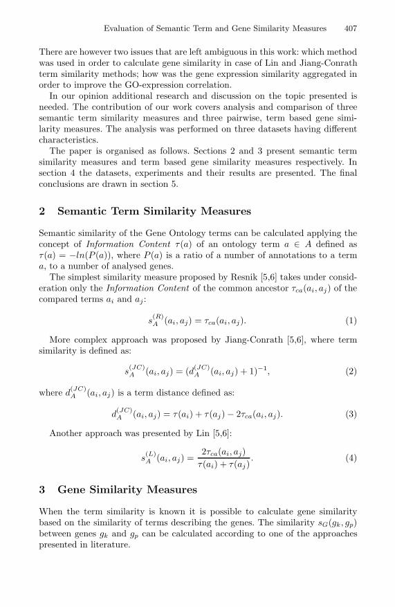
Evaluation of Semantic Term and Gene Similarity Measures 407
There are however two issues that are left ambiguous in this work: which methodwas used in order to calculate gene similarity in case of Lin and Jiang-Conrathterm similarity methods; how was the gene expression similarity aggregated inorder to improve the GO-expression correlation.
In our opinion additional research and discussion on the topic presented isneeded. The contribution of our work covers analysis and comparison of threesemantic term similarity measures and three pairwise, term based gene simi-larity measures. The analysis was performed on three datasets having differentcharacteristics.
The paper is organised as follows. Sections 2 and 3 present semantic termsimilarity measures and term based gene similarity measures respectively. Insection 4 the datasets, experiments and their results are presented. The finalconclusions are drawn in section 5.
2 Semantic Term Similarity Measures
Semantic similarity of the Gene Ontology terms can be calculated applying theconcept of Information Content τ(a) of an ontology term a ∈ A defined asτ(a) = −ln(P (a)), where P (a) is a ratio of a number of annotations to a terma, to a number of analysed genes.
The simplest similarity measure proposed by Resnik [5,6] takes under consid-eration only the Information Content of the common ancestor τca(ai, aj) of thecompared terms ai and aj :
s(R)A (ai, aj) = τca(ai, aj). (1)
More complex approach was proposed by Jiang-Conrath [5,6], where termsimilarity is defined as:
s(JC)A (ai, aj) = (d(JC)
A (ai, aj) + 1)−1, (2)
where d(JC)A (ai, aj) is a term distance defined as:
d(JC)A (ai, aj) = τ(ai) + τ(aj) − 2τca(ai, aj). (3)
Another approach was presented by Lin [5,6]:
s(L)A (ai, aj) =
2τca(ai, aj)τ(ai) + τ(aj)
. (4)
3 Gene Similarity Measures
When the term similarity is known it is possible to calculate gene similaritybased on the similarity of terms describing the genes. The similarity sG(gk, gp)between genes gk and gp can be calculated according to one of the approachespresented in literature.
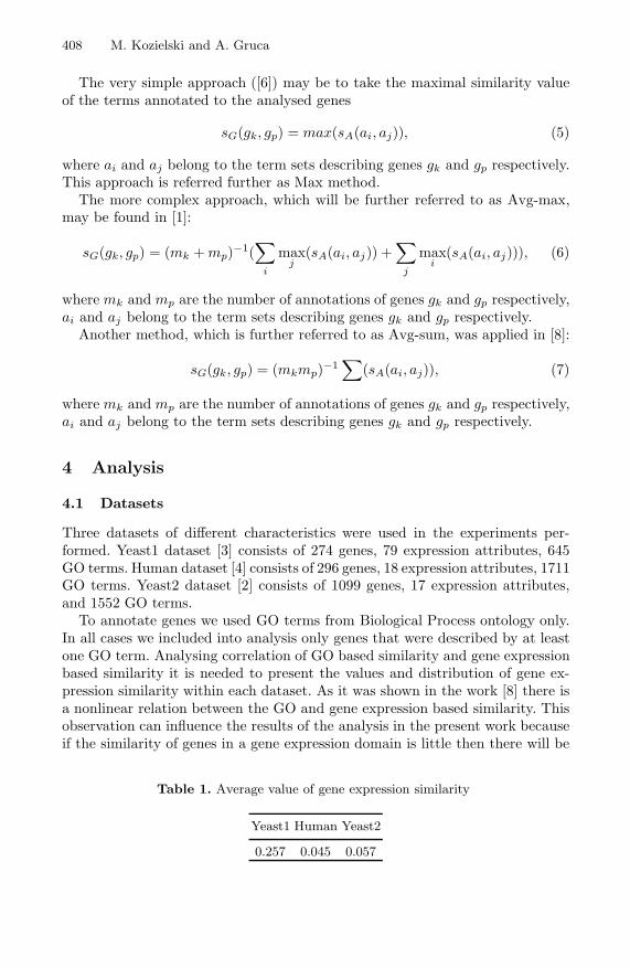
408 M. Kozielski and A. Gruca
The very simple approach ([6]) may be to take the maximal similarity valueof the terms annotated to the analysed genes
sG(gk, gp) = max(sA(ai, aj)), (5)
where ai and aj belong to the term sets describing genes gk and gp respectively.This approach is referred further as Max method.
The more complex approach, which will be further referred to as Avg-max,may be found in [1]:
sG(gk, gp) = (mk + mp)−1(∑
i
maxj
(sA(ai, aj)) +∑
j
maxi
(sA(ai, aj))), (6)
where mk and mp are the number of annotations of genes gk and gp respectively,ai and aj belong to the term sets describing genes gk and gp respectively.
Another method, which is further referred to as Avg-sum, was applied in [8]:
sG(gk, gp) = (mkmp)−1∑
(sA(ai, aj)), (7)
where mk and mp are the number of annotations of genes gk and gp respectively,ai and aj belong to the term sets describing genes gk and gp respectively.
4 Analysis
4.1 Datasets
Three datasets of different characteristics were used in the experiments per-formed. Yeast1 dataset [3] consists of 274 genes, 79 expression attributes, 645GO terms. Human dataset [4] consists of 296 genes, 18 expression attributes, 1711GO terms. Yeast2 dataset [2] consists of 1099 genes, 17 expression attributes,and 1552 GO terms.
To annotate genes we used GO terms from Biological Process ontology only.In all cases we included into analysis only genes that were described by at leastone GO term. Analysing correlation of GO based similarity and gene expressionbased similarity it is needed to present the values and distribution of gene ex-pression similarity within each dataset. As it was shown in the work [8] there isa nonlinear relation between the GO and gene expression based similarity. Thisobservation can influence the results of the analysis in the present work becauseif the similarity of genes in a gene expression domain is little then there will be
Table 1. Average value of gene expression similarity
Yeast1 Human Yeast2
0.257 0.045 0.057

Evaluation of Semantic Term and Gene Similarity Measures 409
Fig. 1. Histogram showing the distribution of the similarity values in gene expressiondomain
little correlation of this similarity with the GO based one. It may be noticedin Table 1 that the average value of gene expression similarity, calculated asa Pearson correlation coefficient, is smaller for Human dataset then for Yeast2dataset, which should result in its worse correlation with Gene Ontology basedsimilarity. However, the distributions presented in Fig. 1 show that for the Hu-man dataset the gene expression similarity has greater variance (the histogramis spread along the whole x axis) comparing to Yeast2 dataset. Thus, the differ-ences in average values can be compensated and it is Human dataset which cangive better results.
4.2 Experiments and Results
The following methods were applied in the experiments. Gene expression basedsimilarity was calculated as Pearson correlation of the expression values.
Gene Ontology annotations were introduced to the analysis by means of binaryarray where ”1” represented annotation of a gene to a term. The annotationtable was constructed in such way that annotation of a gene to a term resultedin annotation of that gene to all the parents of a given term.
GO term similarity was calculated by means of Jiang-Conrath (2), Lin (4)and Resnik (1) methods. Gene similarity was calculated on the basis of termsimilarity by means of Max (5), Avg-max (6) and Avg-sum (7) methods.
The results of the experiments (correlation between gene expression basedand GO based similarity matrices) are presented in the Table 2.
The Max gene similarity is not applicable to Jiang-Conrath and Lin similar-ity measures since it produces in these cases the similarity matrix containingonly a value 1. It results from the fact that if two genes are annotated to theterms having common ancestor, then that ancestor annotates both genes in thecalculated annotation table. Calculating gene similarity as a pairwise term sim-ilarity we have to calculate also self-similarity of such common ancestor. Theself-similarity of a term in case of both Jiang-Conrath and Lin similarity mea-sures equals 1 and this is maximal similarity value that can be calculated. In

410 M. Kozielski and A. Gruca
Table 2. Correlation of gene expression based and GO based similarity
Yeast1 Human Yeast2
Max Resnik 0.257 0.006 -0.013
Avg-maxJiang-Conrath 0.420 0.089 0.015Lin 0.368 0.075 0.005Resnik 0.180 -0.024 0.001
Avg-sumJiang-Conrath 0.383 0.117 0.028Lin 0.352 0.089 0.011Resnik 0.039 -0.068 -0.038
case of Resnik measure the self-similarity of a term is equal to its informationcontent and therefore it is possible to apply the Max method jointly only withResnik measure.
The results show that the method Avg-sum gave the highest absolute cor-relation values in case of two out of three datasets analysed. Considering termsimilarity measures it is Jiang-Conrath that gives the best results in most cases.
The second experiment performed stems from the following two facts men-tioned above: (1) the dependency between gene similarity matrices based onexpression values and on Gene Ontology is not linear, (2) the best correlationbetween such similarity matrices is received when the genes that are highly sim-ilar in expression domain are taken under consideration.
Knowing these two facts we compared the correlation of the full similaritymatrices with the correlation calculated for the matrices indexed by the values ofexpression based similarity se fulfilling the condition se > ε. The values of ε = 0.5and ε = 0.6 were taken under consideration. The results of the experiment, whengene similarity was calculated by means of Avg-sum, are presented in Table 3.
Table 3. Correlation of gene expression based similarity and GO based similarity forthe matrices reduced by ε condition (Avg-sum method); A - full data, B - data reducedfor ε = 0.5, C - data reduced for ε = 0.6
Yeast1 Human Yeast2
A B C A B C A B C
Jiang-Conrath 0.383 0.402 0.334 0.117 0.232 0.304 0.028 0.176 0.298Lin 0.352 0.392 0.323 0.089 0.133 0.192 0.011 0.149 0.256Resnik 0.039 -0.181 -0.224 -0.068 -0.285 -0.355 -0.038 -0.250 -0.385
The results presented in Table 3 show that the dataset reduction appliedimproves in most cases the correlation between the similarity matrices com-pared. It can be also noticed that the results for the Resnik similarity measuregain the greater improvement (when absolute value of a correlation coefficient istaken under consideration) and become better then the results for Jiang-Conrath

Evaluation of Semantic Term and Gene Similarity Measures 411
measure. It can be however disputable if the negatively correlated similaritymatrices can be applied successfully in all types of analysis.
5 Conclusions
The work presented analysis and comparison of three semantic term similaritymeasures and three pairwise, term based gene similarity measures. The analysiswas performed on three datasets having different characteristics.
The results of the experiments showed that Jiang-Conrath and Resnik termsimilarity measures can give the best results of gene expression based similarityand GO based similarity. Jiang-Conrath term similarity measure however, per-forms better on raw data, gives always positively correlated results and seems tobe more suitable for further applications. Considering gene similarity measuresthat were analysed it is Avg-sum method that gives the best results.
References
1. Azuaje, F., Wang, H., Bodenreider, O.: Ontology-driven similarity approaches tosupporting gene functional assessment. In: Proceedings Of The Eighth Annual Bio-Ontologies Meeting, Michigan (2005)
2. Cho, R.J., Campbell, M.J., Winzeler, E.A., Steinmetz, L., Conway, A., Wodicka,L., Wolfsberg, T.G., Gabrielian, A.E., Landsman, D., Lockhart, D.J., Davis, R.W.:A genome-wide transcriptional analysis of the mitotic cell cycle. Mol. Cell 2, 65–73(1998)
3. Eisen, M.B., Spellman, P.T., Brown, P.O., Botstein, D.: Cluster analysis and displayof genome-wide expression patterns. Proc. Natl. Acad. Sci. USA 95, 14863–14868(1998)
4. Iyer, V.R., Eisen, M.B., Ross, D.T., Schuler, G., Moore, T., Lee, J.C., Trent, J.M.,Staudt, L.M., Hudson, J., Boguski, M.S., Lashkari, D., Shalon, D., Botstein, D.,Brown, P.O.: The transcriptional program in the response of human fibroblasts toserum. Science 283, 83–87 (1999)
5. Pesquita, C., Faria, D., Falcao, A.O., Lord, P., Couto, F.M.: Semantic Similarity inBiomedical Ontologies. PLoS Comput. Biol. 5(7), 1–12 (2009)
6. Sevilla, J.L., Segura, V., Podhorski, A., Guruceaga, E., Mato, J.M., Martinez-Cruz,L.A., Corrales, F.J., Rubio, A.: Correlation between gene expression and GO se-mantic similarity. IEEE/ACM Transactions on Computational Biology and Bioin-formaticsm 2(4), 330–338 (2005)
7. Sikora, M., Gruca, A.: Induction and selection of the most interesting Gene On-tology based multiattribute rules for descriptions of gene groups. Pattern Recogn.Letters 32, 258–269 (2011)
8. Wang, H., Azuaje, F., Bodenreider, O., Dopazo, J.: Gene expression correlationand gene ontology-based similarity: an assessment of quantitative relationships. In:Proceedings of the 2004 IEEE Symposium on Computational Intelligence in Bioin-formatics and Computational Biology, CIBCB 2004, pp. 25–31 (2004)

Finding Bicliques in Digraphs: Application into
Viral-Host Protein Interactome
Malay Bhattacharyya1, Sanghamitra Bandyopadhyay1, and Ujjwal Maulik2
1 Machine Intelligence Unit, Indian Statistical Institute203 B. T. Road, Kolkata - 700108, India
malay r,[email protected] Department of Computer Science and Engineering, Jadavpur University
Kolkata - 700032, [email protected]
Abstract. We provide the first formalization true to the best of ourknowledge to the problem of finding bicliques in a directed graph. Theproblem is addressed employing a two-stage approach based on an ex-isting biclustering algorithm. This novel problem is useful in several bi-ological applications of which we focus only on analyzing the viral-hostprotein interaction graphs. Strong and significant bicliques of HIV-1 andhuman proteins are derived using the proposed methodology, which pro-vides insights into some novel regulatory functionalities in case of theacute immunodeficiency syndrome in human.
1 Introduction
The problem of finding bicliques, i.e. complete subgraphs in an undirected bi-partite graph, is a well-known NP-complete problem [4]. Bipartite graphs arerecognized as a triplet (V1, V2, E) in general, where V1, V2 denote two distinctsets of vertices and E ⊆ V1 × V2 is a set of edges. For many real-life appli-cations, directions are also included in graphs depicting regulatory informationand they are formalized as a directed graph (digraph) G, where we distinguishbetween the edges (i, j) and (j, i). In several emerging applications, we are in-terested in exploring biclique-like compact structures in digraphs. In this paper,we formalize the problem of finding bicliques in digraphs. We show that thereis a correspondence between the problem of finding bicliques in digraphs and aspecial type of biclustering. Based on this observation, we propose a method forexploring bicliques in digraphs.
Various studies on gene expression datasets have contributed a lot in the de-velopment of different biclustering algorithms. A quality review of majority ofthe existing biclustering approaches like Cheng and Church’s algorithm (CCA)[3], SAMBA [9], co-clustering, etc. can be found in [8] and [7]. Broadly speaking,biclusters are of four types – fixed value, fixed row/column, additive coherentvalue, and coherent evolution [6]. While SAMBA and co-clustering are designedto find constant value biclusters, CCA can simultaneously find constant valueand constant row/column biclusters. On the other side, SAMBA is able to un-cover overlapping biclusters, while co-clustering (which is designed to only look
S.O. Kuznetsov et al. (Eds.): PReMI 2011, LNCS 6744, pp. 412–417, 2011.c© Springer-Verlag Berlin Heidelberg 2011

Finding Bicliques in Digraphs 413
for disjoint patterns) and Cheng and Church’s method (which masks the iden-tified bicluster with random values in each iteration) can’t find such biclusters.Another divide-and-conquer based biclustering algorithm has recently been pro-posed that pursues inclusion-maximal procedure to prune out all-0 submatricesrecursively from the input binary adjacency matrix to obtain overlapping biclus-ters [8]. This exact algorithm is applicable only to binary data and thus moresuitable to finding bicliques. As can be seen reviewing the literature, only theheuristic algorithm SAMBA has considered the directional changes in expres-sion values while finding statistically significant biclusters. But unfortunately,none of these methods are applicable to directed graphs where directions arealso considered in the graph structure.
In this paper, we revise the methodology proposed in [8] to find out bicliquesin digraphs where all the directions involved in the substructure are mono-directional. We define this as directed bicliques. The problem of finding directedbicliques is formalized in the following section. Sections 4 and 5 describe theproposed methodology and empirical results on the HIV-1-human protein in-teractome (the comprehensive set of interactions) forming a graph structure,respectively. Finally, Section 5 concludes the paper.
2 Problem Definition
A directed bipartite graph, in a generalized form, can be represented as a tripletG = (V1, V2, E), where V1 ∩ V2 = φ and E ⊆ V1 × V2 ∪ V2 × V1. We definea directed biclique, hereafter referred as DBClique, as a complete subgraph of adirected bipartite graph as per the following.
Definition 1 (DBClique). A DBClique is a fully connected subgraph G′ =(V ′
1 , V ′2 , E′) ⊆ G of a directed bipartite graph G such that either i ∈ V ′
1 , j ∈V ′
2 , ∀(i, j) ∈ E′ or i ∈ V ′2 , j ∈ V ′
1 , ∀(i, j) ∈ E′.
A directed bipartite graph is shown in Fig. 1(a) in which the sets of vertices II,III and 2, 3, 4 form a DBClique. Notably, this corresponds to a special kindof constant value biclusters. If we construct an interaction matrix (as shown inFig. 1(b)) from the directed bipartite graph in Fig. 1(a), it somehow correspondsto an all-1 submatrix, but not an exact one. We provide a lemma to highlighta correspondence between the problem of finding DBCliques and a variant ofbiclustering. For this, let us first define the matrix representation of a directedbipartite graph as follows.
Definition 2 (Interaction matrix of a directed bipartite graph). Theinteraction matrix of a directed bipartite graph G = (V1, V2, E) is defined as a|V1| × |V2| matrix I such that
Iij =
⎧⎪⎪⎨
⎪⎪⎩
0, if (i, j) /∈ E and (j, i) /∈ E1, if (i, j) ∈ E and (j, i) /∈ E−1, if (i, j) /∈ E and (j, i) ∈ EX, if (i, j) ∈ E and (j, i) ∈ E
,
∀i ∈ V1, j ∈ V2.

414 M. Bhattacharyya, S. Bandyopadhyay, and U. Maulik
(a) (b)
Fig. 1. The one-to-one correspondence between a single (a) DBClique in a directedbipartite graph and (b) a special kind of bicluster in its representative interactionmatrix reflected as a submatrix
An example interaction matrix is shown in Fig. 1(b). The character ‘X ’ inthe matrix I defined beforehand is behaviorally a don’t care entry. Based on thisrepresentation, we can equate a DBClique to a bicluster through the followinglemma.
Lemma 1. Given a directed bipartite graph G = (V1, V2, E), a DBClique G′ =(V ′
1 , V ′2 , E′) ⊆ G corresponds to a bicluster in the interaction matrix of G such
that all the elements in the submatrix are either ‘1’ or ‘-1’, with the entries of‘X’ additionally allowed.
Proof. Certainly, an entry ‘X ’ in any submatrix of a bicluster represents both‘1’ and ‘-1’. Thus, a bicluster with all the entries either ‘1’ or ‘X ’ will correspondto an edge (i, j) directed from V1 to V2. Equivalently, a bicluster with all ‘-1’ or‘X ’ will correspond to an edge (i, j) directed from V2 to V1. Thus the lemma. Our motivation is to find out the set of maximal DBCliques from a given directedbipartite graph.
3 Proposed Method
We describe the two-stage algorithm to find out DBCliques in digraphs usingthe previous lemma. The methodology is based on the Bimax algorithm [8].The approach for finding out maximal overlapping DBCliques (all ‘1’ and all ‘-1’biclusters) is described in detail in Algorithm 1. The key step in this algorithm ispursuing separate phases (steps 2-5 and steps 6-9) for finding out the regulating(all ‘1’) and regulated (all ‘-1’) DBCliques. After this, we apply a divide-and-conquer process (adopted in [9]) to find out the maximal DBCliques from thegiven directed bipartite graph.
4 Experimental Results
To demonstrate the effectiveness of the methodology, we collect the interactioninformation (5134 interactions in total) between 19 HIV-1 and 1448 human pro-teins as reported in a recently published dataset [5]. It consists of two types

Finding Bicliques in Digraphs 415
Algorithm 1. An Algorithm for Finding out Bicliques in DigraphsInput: A directed bipartite graph G = (V1, V2, E).Output: The set of maximal DBCliques.Steps of the algorithm:
1: Obtain the correspondent interaction matrix I from G2: Replace the entries ‘X’ with ‘1’ and ‘-1’ with ‘0’ in I // Finding the all ‘1’ biclusters3: Partition I = I0 ∪ I1 ∪ I2 such that the size of I0 maximizes and it contains only 0’s.4: Go to the previous step and apply the same individually on I1 and I2 until no further partitioning
is possible.5: Return the DBCliques corresponding to the biclusters6: Replace the entries ‘X’ with ‘-1’ and ‘1’ with ‘0’ in I // Finding the all ‘-1’ biclusters7: Partition I = I0 ∪ I1 ∪ I2 such that the size of I0 maximizes and it contains only 0’s.8: Go to the previous step and apply the same individually on I1 and I2 until no further partitioning
is possible.9: Return the DBCliques corresponding to the biclusters
of interactions, viz., direct physical interactions and indirect interactions, cat-egorized into 65 more specific types. The corresponding bipartite graph thuscontains 19 vertices representing HIV-1 proteins and 1448 vertices representinghuman proteins, and 5134 edges representing the viral-host interactions. Theinteraction matrix of size 19× 1448 corresponding to the bipartite graph is con-structed. All the 65 interaction types are biologically classified into three types –regulating, regulated by and two-way (where the regulation is bidirectional). Asper this, an entry ‘0’ in the matrix denotes the absence of interaction between thecorresponding pair of HIV-1 and human proteins, an entry of ‘1’ represents theregulation of the HIV-1 protein on the human protein, an entry of ‘-1’ denotesthat the HIV-1 protein is regulated by the human protein and ‘X ’ representsa two-way interaction. Now, to find out the all ‘1’ and all ‘-1’ biclusters fromthis, we applied the element-replacement strategies (steps 2 and 6) given in Al-gorithm 1 and the resulting binary matrices are processed further.
The available codes of Bimax biclustering method, as implemented in theBicAT toolbox [1], is employed to iteratively find out the matrix partitions ofthe binary data matrices. The lower bound of HIV-1 and human protein sizesare both set to 3 for obtaining a bicluster, i.e., we aim to find only those DB-Cliques which contain at least 3 HIV-1 proteins and 3 human proteins. Withthis restriction, the numbers of all ‘1’ and all ‘-1’ DBCliques are found to be 113and 25, respectively. Further neglecting don’t care entries in these matrices, weended up with 54 and 7 strong DBCliques, respectively for the all ‘1’ and all ‘-1’cases. Several of these bicliques forms a strong (with high clustering co-efficient)bipartite subgraph which contains the HIV-1 proteins like env gp120, pol RT,tat, etc. On the other side, many of the human proteins like CD4, LCK, MAPK1etc. and also several kinase proteins are obtained within this module. There areseveral literature evidences where CD4 has been reported as an important cellmembrane protein that act as the receptor and co-receptor for the viral entry,respectively [2]. The details of the DBCliques obtained are listed in Table 1.
The all ‘1’ and all ‘-1’ submatrices obtained are nothing but the representa-tives of strong modulated regulation between two sets of proteins. It becomesevident from the maximum sizes of the DBCliques that the immunodeficiencysignal passing in either directions between HIV-1 and human proteins are equally

416 M. Bhattacharyya, S. Bandyopadhyay, and U. Maulik
Table 1. The DBCliques obtained from the HIV-1-human protein interaction networkcontaining at least three HIV-1 and human proteins each. The size of a DBClique isdefined based on the number of edges it contains.
Bicluster type Don’t care allowed # DBCliques obtained Maximum size(HIV-1, Human)
All ‘1’ Yes 113 (6, 5)All ‘-1’ Yes 25 (3, 13)All ‘1’ No 54 (4, 5)All ‘-1’ No 7 (3, 8)
significant. Further analysis from the Gene Ontology (GO) also shows the sig-nificant p-values (< 1.0E−3) for several of the DBCliques obtained representinghighly coherent groups of regulatory functional proteins. As for example, considerthe largest-sized and strong DBClique corresponding to the all ‘-1’ bicluster. Itconsists of three HIV-1 proteins tat, env gp120 and matrix, and eight heat shock70kDa proteins (1A, 1B, 2, 4, 5, 6, 8 isoform 1 and 9 precursor) of human. Theseproteins are generally expressed when cells are exposed to elevated temperaturesor other stresses likewise the entry of viral proteins. In fact, the env gp120 pro-tein is associated with the insertion of viral proteins in the host body in case ofAIDS. Thus, this substructure is a biologically significant regulatory module inpassing the immunodeficiency signal in human.
We have further carried out relative studies between the proposed methodand several other algorithms to show the enhanced biological significance of theDBCliques in comparison with the conventional bicliques. All these algorithmsare applied on the binary data matrix obtained from the interaction networkignoring directions. The comparative results are shown in Table 2. Notably,every biclique is a DBClique but not the vice versa, and therefore DBCliquesinclude additional information in their substructures. This is reflected from thebetter p-values obtained representing more biological coherence for DBCliquesas compared to the bicliques. In fact, some of these results appear to be veryinsignificant producing poor p-values (> 1.0E−2). Thus, it appears that theDBCliques are significant substructures in a regulatory biological network.
Table 2. Comparison of the largest bicliques (consisting of at least three HIV-1 andhuman proteins) derived by various algorithms from the HIV-1-human protein inter-action network. The proposed method exclude the Don’t care conditions and returnsDBCliques. Crossed cells in the third column represent insignificant p-values.
Analytical details Bimax CC ISA Proposed
# Bicliques obtained 197 60 10 61Largest biclique found (4, 9) (19, 392) (5, 76) (3, 8)Best p-value from GO 1.9E−6 × × 2.3E−12
Best annotation Regulation of cytokinesis Not Not Response to protein(GO Term) (GO:0032465) applicable applicable stimulus (GO:0051789)

Finding Bicliques in Digraphs 417
5 Concluding Remarks
The problem of finding bicliques in directed bipartite graphs is addressed in thispaper based on an optimal biclustering algorithm. We provide exact solutions tothis problem and it is demonstrated that the problem reduces to a special classof biclustering problem. The analysis on the interaction network of HIV-1 andhuman proteins demonstrates the effectiveness of the proposed methodology andits usefulness.
Acknowledgments
A part of the work was carried out when S. Bandyopadhyay visited the MaxPlanck Institute for Informatics, Saarbrucken, Germany, and U. Maulik visitedthe German Cancer Research Center, Heidelberg, Germany, with Humboldt Fel-lowship for Experienced Researchers in 2010.
References
1. Barkow, S., Bleuler, S., Prelic, A., Zimmermann, P., Zitzler, E.: BicAT: a Bicluster-ing Analysis Toolbox. Bioinformatics 22(10), 1282–1283 (2006)
2. Brass, A.L., Dykxhoorn, D.M., Benita, Y., Yan, N., Engelman, A., Xavier, R.J.,Lieberman, J., Elledge, S.J.: Identification of Host Proteins Required for HIV Infec-tion Through a Functional Genomic Screen. Science 319(5865), 921–926 (2008)
3. Cheng, Y., Church, G.: Biclustering of Expression Data. In: Proceedings of the 8thISMB Conference, AAAI Press, pp. 93–103. AAAI Press, Menlo Park (2000)
4. Ding, C., Zhang, Y., Li, T.: Biclustering Protein Complex Interactions with a Bi-clique Finding Algorithm. In: Proceedings of the Sixth International Conference onData Mining, Hong Kong, pp. 178–187 (2006)
5. Fu, W., Sanders-Beer, B.E., Katz, K.S., Maglott, D.R., Pruitt, K.D., Ptak, R.G.: Hu-man immunodeficiency virus type 1, human protein interaction database at NCBI.Nucleic Acids Research 37(Database Issue), D417–D422 (2009)
6. Madeira, S.C., Oliveira, A.L.: Biclustering algorithms for biological data analysis: asurvey. IEEE/ACM Transactions on Computational Biology and Bioinformatics 1,24–45 (2004)
7. Pandey, G., Atluri, G., Steinbach, M., Myers, C.L., Kumar, V.: An AssociationAnalysis Approach to Biclustering. In: Proceedings of the 15th ACM SIGKDD Con-ference on Knowledge Discovery and Data Mining, Paris, France (2009)
8. Prelic, A., Bleuler, S., Zimmermann, P., Wille, A., Buhlmann, P., Gruissem, P.,Hennig, L., Thiele, L., Zitzler, E.: A systematic comparison and evaluation of bi-clustering methods for gene expression data. Bioinformatics 22(9), 1122–1129 (2006)
9. Tanay, A., Sharan, R., Shamir, R.: Discovering statistically significant biclusters ingene expression data. Bioinformatics 18, S136–S144 (2002)

Advantages of the Extended Water Flow
Algorithm for Handwritten Text Segmentation
Darko Brodic
University of Belgrade, Technical Faculty Bor,V. J. 12, 19210 Bor, [email protected]
Abstract. This paper identifies the advantages of the specific approachto water flow algorithm for multi-skewed handwritten text line segmen-tation. Original water flow algorithm assumes that hypothetical waterflows, from both left and right sides of the document image frame, faceobstruction from part of character, character, and group of charactersin text lines. The stripes of areas left unwetted on the document imageframe are finally labeled for the extraction of text lines. However, themethod defines parameter water flow angle for flooding which dependson the text line slopes of each specific document. The estimation of theappropriate parameter value is difficult and limited as well. The limita-tion is manifested by possible election of only 4 values for this parameter.Extended approach has introduced enlargement of the parameter range.Consequently, decision making and the selection of the small values ofthe parameter below the minimum given by the original method showsimprovement in the handwritten text line segmentation process. It isconfirmed by the measurement on different types of letters.
Keywords: Image processing; Document image processing; Text linesegmentation; Handwritten text; Water flow algorithm.
1 Introduction
Text line segmentation of handwritten text is a key element of the optical char-acter recognition [1]. It implies a labeling process that assign the same label tospatially aligned units, connected components or characteristic points [1]. Fur-ther, based on the obtained labels, text is divided into different regions each onerepresenting text line. After text line segmentation is finished, it provides theessential information for the consecutive documents image steps such as baselinedetection, skew identification and correction, other text feature extraction andcharacter recognition.
Related work on text line segmentation can be categorized in few directions[1,2]: projection based methods, Hough transform methods, grouping methods,methods for processing overlapping and touching components, stochastic meth-ods, smearing methods, and others method.
In smearing methods the consecutive black pixels along the horizontal direc-tion are smeared [3]. Consequently, the white space between black pixels is filled
S.O. Kuznetsov et al. (Eds.): PReMI 2011, LNCS 6744, pp. 418–423, 2011.c© Springer-Verlag Berlin Heidelberg 2011

Advantages of the Extended Water Flow Algorithm 419
with black pixels. It is valid only if their distance is within a predefined thresh-old. This way, enlarged area of black pixels around text is formed. It is so-calledboundary growing area. Hence, the smeared image encloses text lines.
As mentioned many methods can be employed for text line segmentation, butsmearing algorithms have the benefits. They are efficient and computationallyinexpensive. Algorithm proposed in [4] is classified as smearing method. It as-sumed a hypothetical flow of water in a particular direction across image framein a way that it faces obstruction from the characters of the text lines. As a re-sult of algorithm, unwetted image frames are extracted. These areas are of majorimportance for text line segmentation. In our paper, this algorithm is extendedas well as in [5,6] and further investigated, improved and adapted.
The rest of the paper is organized as follows: Section 2 describes basic wa-ter flow algorithm and introduces extended approach to water flow algorithm.Section 3 defines testing process and shows measurement results including com-parative analysis. Section 4 makes conclusions.
2 Water Flow Algorithm
Document text image is obtained as result of scanning process. It is grayscaletext image described by intensity matrix D(i ,j ) ∈ 0,. . .,255 , where i ∈ 1, M and j ∈ 1, N [7]. After applying intensity segmentation with binarization, it isconverted into binary image X (i ,j ). Hence, where D(i ,j ) ≥ Dth , then X (i ,j ) is1, elsewhere X (i ,j ) is 0. Consequently, Dth represents the threshold sensitivitydecision value. It is obtained by global [8] or local binarization method [9,10,11].
Basic water flow algorithm [4] assumes hypothetical water flows under fewangles of the document image frame from left to right and vice versa. In thishypothetically assumed situation, water is flowing across the image frame. Areasthat are not wetted form unwetted ones. The stripes of unwetted areas are labeledfor the extraction of text lines. Further, this hypothetical water flow is expectedto fill up the gaps between text elements in the same text lines. Hence, unwettedareas left on the image frame lies under the text lines. Once the labeling iscompleted, the image is divided into two different types of stripes. First onecontains text lines. The other one contains space between text lines. Furthermore,water flow angle α, as shown in Fig.1, is introduced as a referent parameter in[4]. This angle is measured between two lines which intersect each other at theendpoint of an obstacle. However, it is formed by labeling original documentimage using spatial filter mask. These masks for the water flows from left toright are shown in Fig.1.
Accordingly, algorithm creates unwetted areas under fixed water flow anglesfrom the set 14, 18, 26.6, 45 [4]. Using of the spatial filter masks is definedby the position of the text black pixels. They represent prospective seed points.If the pixel represents corner one, then the spatial filter mask will be exploited.Thus, it activates the algorithm process. As the result, unwetted stripes boundedtext. This circumstance for α = 26.6 is shown in Fig.2.
In the extended approach, originally extraction of the rectangular boundingbox over the text objects is prerequisite. Further, they represent control areas

420 D. Brodic
Fig. 1. Spatial filter mask defined by water flow angle: α = 45 (left), α = 26.6 (middleleft), α = 18 (middle right), and α = 14 (right)
Fig. 2. Water flow algorithm with water flow angle α = 26.6 : Initial sample textcontaining four I letters (top), unwetted areas made by water flow from left to right(middle left), unwetted areas made by water flow from right to left (middle right), andunited unwetted areas (bottom).
authorized for the extended water flow algorithm criteria activation. Boundingbox is a rectangular region whose edges are parallel to the coordinate axes. It isdefined by its endpoints: xmin , ymin , xmax , and ymax . Hence, each pixel X (i ,j )that belongs to the bounding box is given by [12]:
X (i , j ) | (xmin ≤ i ≤ xmax ) ∧ (ymin ≤ j ≤ ymax ). (1)
Inclusion of the point X (i ,j ) in the bounding box is tested by verifying thesefour inequalities. If any one of them fails, then the point is not inside [13]. Alltext objects like letters, part of words or words are surrounded by boundingboxes [14]. It should be noted that from this point all actions are referred onlyto text in each independent bounding box.
Apart from original algorithm procedure, unwetted areas could be determinedby lines. Each line is defined as:
y = ax + b, (2)
where slope a = tan(α). Two lines defined by angle α make connection inspecific pixel creating closed unwetted area [5,6].

Advantages of the Extended Water Flow Algorithm 421
Modification made on water flow algorithm is in its definition. Consequently,it forms the water flow function which determines the water flow angle α. Still,making straight lines from boundary pixel type and connecting each others inspecified point makes unwetted region as well. Currently, modified water flowalgorithm is open to choose different water flow angle from 0 to 90. In addi-tion, different decision-making process on boundary text pixels is made. Fig.3illustrates these circumstances [5,6].
Fig. 3. Pixel type determination: upper boundary pixel (left), lower boundary pixel(middle), and boundary pixel for additional investigation (right)
Due to pixel type, the slope is -α or +α. However, pixel without completelocation has been additionally investigated. It depends on neighbor area of pixels.Apart from [5], enlarged window composed of R x S pixels, defined as a basis.In [6] R = 5 and S = 7 is proposed for complete investigation.
The main achievement of unwetted area is text line segmentation. However,the problem originates in broken words of text lines. Algorithm should contributeto join those words by unwetted areas. Those areas can be lengthen by usingsmaller angle α. This is represented in Fig.4.
Fig. 4. Extended water flow algorithm involving water flow function y = ax + b definingand bounding boxes surrounding text (box with dotted lines)
3 Testing, Results and Comparative Analysis
The proposed approach was tested using a group of binary handwritten docu-ments images. These documents were written in English as well as in SerbianLatin and Cyrillic letters. The total number of analyzed handwritten text lineswas 220. For the sake of conformity, documents body is the only considered inthe analysis of the line segmentation.
Table 1 presents the number of correctly segmented text lines as well as dif-ferent types of segmented errors. Errors are divided in 3 groups: split lines error,joined lines error, and lines including outlier words [15].
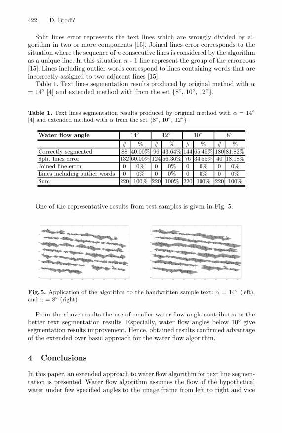
422 D. Brodic
Split lines error represents the text lines which are wrongly divided by al-gorithm in two or more components [15]. Joined lines error corresponds to thesituation where the sequence of n consecutive lines is considered by the algorithmas a unique line. In this situation n - 1 line represent the group of the erroneous[15]. Lines including outlier words correspond to lines containing words that areincorrectly assigned to two adjacent lines [15].
Table 1. Text lines segmentation results produced by original method with α= 14 [4] and extended method with from the set 8, 10, 12.
Table 1. Text lines segmentation results produced by original method with α = 14
[4] and extended method with α from the set 8, 10, 12
Water flow angle 14 12 10 8
# % # % # % # %
Correctly segmented 88 40.00% 96 43.64% 144 65.45% 180 81.82%
Split lines error 132 60.00% 124 56.36% 76 34.55% 40 18.18%
Joined line error 0 0% 0 0% 0 0% 0 0%Lines including outlier words 0 0% 0 0% 0 0% 0 0%
Sum 220 100% 220 100% 220 100% 220 100%
One of the representative results from test samples is given in Fig. 5.
Fig. 5. Application of the algorithm to the handwritten sample text: α = 14 (left),and α = 8 (right)
From the above results the use of smaller water flow angle contributes to thebetter text segmentation results. Especially, water flow angles below 10 givesegmentation results improvement. Hence, obtained results confirmed advantageof the extended over basic approach for the water flow algorithm.
4 Conclusions
In this paper, an extended approach to water flow algorithm for text line segmen-tation is presented. Water flow algorithm assumes the flow of the hypotheticalwater under few specified angles to the image frame from left to right and vice

Advantages of the Extended Water Flow Algorithm 423
versa. Instead of using limited choices of parameter called water flow angle, newapproach introduced approach to freely choose this parameter. Furthermore,choosing smaller water flow angles contributes to the enlarged unwetted areawhich leads to better text line segmentation results. It is upheld by testing withthe group of handwritten documents in Serbian and English language. Hence,the extended approach of the water flow algorithm confirms better text linesegmentation ability.
References
1. Likforman-Sulem, L., Zahour, A., Taconet, B.: Text Line Segmentation of HistoricalDocuments: A Survey. IJDAR 9(2-4), 123–138 (2007)
2. Amin, A., Wu, S.: Robust Skew Detection in Mixed Text/Graphics Documents.In: 8th ICDAR, Seoul, Korea, pp. 247–251 (2005)
3. Shi, Z., Govindaraju, V.: Line Separation for Complex Document Images usingFuzzy Runlength. In: Int. Workshop on Document Image Analysis for Libraries,Palo Alto, USA, pp. 306–312 (2004)
4. Basu, S., et al.: Text Line Extraction from Multi-skewed Handwritten Documents.Pattern Recognition 40(6), 1825–1839 (2007)
5. Brodic, D., Milivojevic, Z.: An Approach to Modification of Water Flow Algo-rithm for Segmentation and Text Parameters Extraction. In: Camarinha-Matos,L.M., Pereira, P., Ribeiro, L. (eds.) IFIP AICT, vol. 314, pp. 323–331. Springer,Heidelberg (2010)
6. Brodic, D., Milivojevic, Z.: Text Line Segmentation by Adapted Water Flow Al-gorithm. In: 10th Symposium NEUREL, Belgrade, Serbia, pp. 225–229 (2010)
7. Gonzalez, R.C., Woods, R.E.: Digital Image Processing, 2nd edn. Prentice-Hall,Englewood Cliffs (2002)
8. Otsu, N.: A Threshold Selection Method from Gray-level Histograms. IEEE Tran.on Systems, Man, and Cybernetics 9(1), 62–66 (1979)
9. Sauvola, L., Pietikainen, M.: Adaptive Document Image Binarization. PatternRecognition 33(2), 225–236 (2000)
10. Bukhari, S.S., Shafait, F., Bruesl, T.M.: Adaptive Binarization of UnconstrainedHand-held Camera-captured Document Images. J. of Universal Computer Sci-ence 15(18), 3343–3363 (2009)
11. Khashman, A., Sekeroglu, B.: Document Image Binarisation Using a SupervisedNeural Network. Int. J. of Neural Systems 18(5), 405–418 (2008)
12. Preparata, F.P., Shamos, M.I.: Computational Geometry: An Introduction.Springer, Berlin (1985)
13. Chang, C.M.: Detecting Ellipses via Bounding Boxes. Asian Journal of Health andInformation Sciences 1(1), 73–84 (2006)
14. Wang, J., Leung, M.K.H., Hui, S.C.: Cursive Word Reference Line Detection. Pat-tern Recognition 30(3), 503–511 (1997)
15. Sanchez, A., et al.: Text Line Segmentation in Images of Handwritten HistoricalDocuments. In: 1st IPTA, Sousse, Brasil, pp. 1–6 (2008)
Construction of Model of Structured Documents
Based on Machine Learning
Sergey Golubev1,2
1 Moscow Institute of Physics and Technology, Dolgoprudny, Russia2 ABBYY Software, Moscow, Russia
Gergey [email protected]
Abstract. In this paper we consider the problem of structured docu-ment recognition. The document recognition system is proposed. Thissystem incorporates a recognition module based on methods of struc-tured image recognition, a graph document model and a method of doc-ument model generalization. The machine learning component makes theprocess of document model construction easier and less time-consuming.
Keywords: document recognition, machine learning, graph documentmodel.
1 Introduction
The extensive development of information technologies and electronic documentmanagement systems poses the problem of converting paper documents into digi-tal form. While modern OCR systems can recognize symbols with high precision,simple character recognition is often insufficient. To capture the data correctly,a recognition of logical document structure is needed. The most precise and flex-ible methods of recognition of document structure are those based on structuredpattern recognition [1,2]. These methods use the model of document structurewhich is compared to the document image during recognition.
The most widespread document model is the graph model where text blocksand separator lines form graph vertices, whereas graph edges correspond to re-lations between them [3]. The recognition problem in this case is the problemof matching of two graphs: the model graph and the document graph which isformed from the document image prior to recognition process. Systems based ongraph models often allows automatic construction of document model based onmethods of machine learning.
Another document recognition system based on the methods of structuredpattern recognition is the ABBYY FlexiLayout system [4]. This system usesmore complex special-purpose document model (structural description). In com-parison with graph based methods the FlexiLayout system can reach higherrecognition quality especially for documents with complex structure. The maindrawback of the ABBYY FlexiLayout system is that the document descriptionis designed to be created manually which is difficult and time-consuming. It
S.O. Kuznetsov et al. (Eds.): PReMI 2011, LNCS 6744, pp. 424–431, 2011.c© Springer-Verlag Berlin Heidelberg 2011

Construction of Model of Structured Documents Based on Machine Learning 425
seems reasonable to combine the FlexiLayout document recognition system withthe methods of machine learning. This allows us to take advantage of both theprecision of the FlexiLayout system and the easy constructing of graph baseddocument model. We propose a trainable system for document recognition whichincorporates the FlexiLayuot recognition module and a training module. Thetraining module uses an intermediate graph document model on the trainingstage. The graph model is then converted into the FlexiLayout document descrip-tion. In this paper we will discuss the graph document model and the process ofits construction.
2 Problem Setting
In this work a special class of documents, so called forms, is discussed. Thedistinctive feature of this document class is that the document structure consistsof the static part (which is presented by headings, separator lines etc.) and dataelements. The examples of forms are various questionaries, financial documentslike invoices, payment orders, etc.
All forms can be divided in four classes in terms of structure complexity: fixedforms, semi-fixed forms, flex-forms and free forms. A fixed form is a documentthat maintains all characteristics of its layout (except for scanning distortionssuch as stretching, skew etc.). The recognition of fixed-forms is a relatively sim-ple task and does not require structure recognition. Semi-fixed forms are createdfrom fixed-forms by relaxing some restrictions on the document layout. An exam-ple of semi-fixed form is an electronic template which allows to move succeedingdata fields, if more space is needed for the given field or section. The recogni-tion of semi-fixed forms can be performed using table or graph based documentmodels. In a flex-form (also called context-form) each data element has an identi-fiable local context associated with it. The data element and the related contextmay be located in varying places on the document image. However, the rela-tive position of the data element to its context is relatively constant. Free formsinclude documents which are not fixed, semi-fixed or flex-forms, extraction ofdata from this documents may require advanced natural language processing. Incurrent paper we will consider the first three types of forms: fixed, semi-fixedand flex-forms.
The problem of form recognition is the following: given a document imagethe system must detect the localization of data elements so as to recognize therequired data (using OCR technologies) and input it into the database. Thesystem uses certain number of document images with marked locations of dataelements as training set. After the training process the system must be able tolocate the data elements on any other document image of the same documenttype.
The recognition problem is solved in two stages. On the first stage a modelis generated on the base of training examples, on the second stage this model isused to solve recognition (prediction, classification) problem. In our work we usethe ABBYY FlexiLayout system as a recognition module. Thereby the model is

426 S. Golubev
the FlexiLayout structural description (for more information on structural de-scriptions see [4]). The FlexiLayout document model contains the descriptionsof the document structural elements. The description of each structural elementdefines its attributes, allowing to detect the structural element on the docu-ment image. Unlike the graph based methods the FlexiLayout system does notuse a priori extraction of structural elements. Instead, structural elements aredetected directly during the recognition process according to the document de-scription and taking into account the particular features of a document type.Particularly important feature of the system is the ability to calculate attributesof structural elements and relations between them “on the fly”. For examplethe distance between two elements may be calculated using the size of detectedrectangle of one of the elements. The relative positions of structural elementsare described in the model in terms of metrical and ordering relations. In thisrespect the FlexiLayout model is similar to graph models. In fact a graph modelwith metrical relations may be converted into the FlexiLayout description if thelabels of graph vertices have the appropriate format. The FlexiLayuot modelalso supports fuzzy relations between elements.
The document description uses a specialized language to describe attributes ofstructural elements and relations between them. Therefore it is not convenientfor machine learning and it was designed mainly to be created manually bysystem operator. Therefore, it is preferable to use a simpler graph model on thestage of model generation. When the intermediate graph model is generated inthe learning process it is then converted into FlexiLayout structural description.FlexiLayout description in then used for document recognition. In the followingsection we will discuss the intermediate graph document model and the methodof its generalization.
3 Document Model
In structural pattern recognition methods it is convenient to represent the doc-ument image as a set of image objects. The input document image is a rasterimage obtained by scanning the paper document. This image is subjected tosegmentation process which extracts connected pixel components. Connectedcomponents are the images of separate letters, punctuation symbols, parts of sep-arator lines and pictures. Each connected component is classified and recognized(if it represents letter). We use classified and recognized connected componentsas elementary image objects. The elementary image object is described by itstype, surrounding rectangle and Unicode code of recognized symbol (for letters,diacritics and punctuation symbols). The image object is either an elementaryobject or a combination of elementary objects.The complex image object is de-scribed by its constituents. The following hierarchy of image objects is used:
1. Letter → Word → Text line → Text fragment2. Separator fragment → Separator line3. Picture fragment → Picture
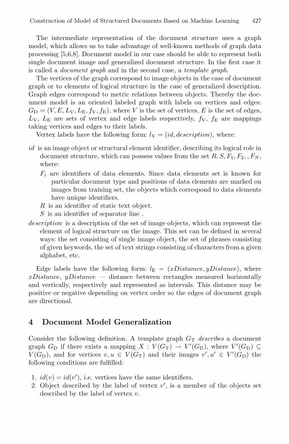
Construction of Model of Structured Documents Based on Machine Learning 427
The intermediate representation of the document structure uses a graphmodel, which allows us to take advantage of well-known methods of graph dataprocessing [5,6,8]. Document model in our case should be able to represent bothsingle document image and generalized document structure. In the first case itis called a document graph and in the second case, a template graph.
The vertices of the graph correspond to image objects in the case of documentgraph or to elements of logical structure in the case of generalized description.Graph edges correspond to metric relations between objects. Thereby the doc-ument model is an oriented labeled graph with labels on vertices and edges:GD = (V, E, LV, LE, fV, fE), where V is the set of vertices, E is the set of edges,LV, LE are sets of vertex and edge labels respectively, fV, fE are mappingstaking vertices and edges to their labels.
Vertex labels have the following form: lV = (id, description), where:
id is an image object or structural element identifier, describing its logical role indocument structure, which can possess values from the set R, S, F1, F2, , FN ,where:Fi are identifiers of data elements. Since data elements set is known for
particular document type and positions of data elements are marked onimages from training set, the objects which correspond to data elementshave unique identifiers.
R is an identifier of static text object.S is an identifier of separator line .
description is a description of the set of image objects, which can represent theelement of logical structure on the image. This set can be defined in severalways: the set consisting of single image object, the set of phrases consistingof given keywords, the set of text strings consisting of characters from a givenalphabet, etc.
Edge labels have the following form: lE = (xDistamce, yDistance), wherexDistance, yDistance — distance between rectangles measured horizontallyand vertically, respectively and represented as intervals. This distance may bepositive or negative depending on vertex order so the edges of document graphare directional.
4 Document Model Generalization
Consider the following definition. A template graph GT describes a documentgraph GD if there exists a mapping X : V (GT) → V ′(GD), where V ′(GD) ⊆V (GD), and for vertices v, u ∈ V (GT) and their images v′, u′ ∈ V ′(GD) thefollowing conditions are fulfilled:
1. id(v) = id(v′), i.e. vertices have the same identifiers.2. Object described by the label of vertex v′, is a member of the objects set
described by the label of vertex v.
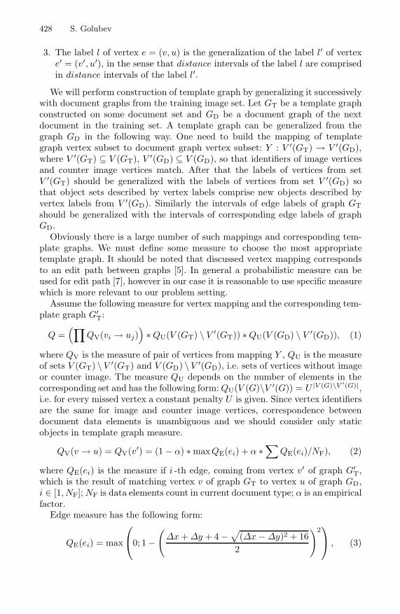
428 S. Golubev
3. The label l of vertex e = (v, u) is the generalization of the label l′ of vertexe′ = (v′, u′), in the sense that distance intervals of the label l are comprisedin distance intervals of the label l′.
We will perform construction of template graph by generalizing it successivelywith document graphs from the training image set. Let GT be a template graphconstructed on some document set and GD be a document graph of the nextdocument in the training set. A template graph can be generalized from thegraph GD in the following way. One need to build the mapping of templategraph vertex subset to document graph vertex subset: Y : V ′(GT) → V ′(GD),where V ′(GT) ⊆ V (GT), V ′(GD) ⊆ V (GD), so that identifiers of image verticesand counter image vertices match. After that the labels of vertices from setV ′(GT) should be generalized with the labels of vertices from set V ′(GD) sothat object sets described by vertex labels comprise new objects described byvertex labels from V ′(GD). Similarly the intervals of edge labels of graph GT
should be generalized with the intervals of corresponding edge labels of graphGD.
Obviously there is a large number of such mappings and corresponding tem-plate graphs. We must define some measure to choose the most appropriatetemplate graph. It should be noted that discussed vertex mapping correspondsto an edit path between graphs [5]. In general a probabilistic measure can beused for edit path [7], however in our case it is reasonable to use specific measurewhich is more relevant to our problem setting.
Assume the following measure for vertex mapping and the corresponding tem-plate graph G′
T:
Q =(∏
QV(vi → uj))∗ QU(V (GT) \ V ′(GT)) ∗ QU(V (GD) \ V ′(GD)), (1)
where QV is the measure of pair of vertices from mapping Y , QU is the measureof sets V (GT) \ V ′(GT) and V (GD) \ V ′(GD), i.e. sets of vertices without imageor counter image. The measure QU depends on the number of elements in thecorresponding set and has the following form: QU(V (G)\V ′(G)) = U |V (G)\V ′(G)|,i.e. for every missed vertex a constant penalty U is given. Since vertex identifiersare the same for image and counter image vertices, correspondence betweendocument data elements is unambiguous and we should consider only staticobjects in template graph measure.
QV(v → u) = QV(v′) = (1 − α) ∗ maxQE(ei) + α ∗∑
QE(ei)/NF), (2)
where QE(ei) is the measure if i -th edge, coming from vertex v′ of graph G′T,
which is the result of matching vertex v of graph GT to vertex u of graph GD,i ∈ [1, NF]; NF is data elements count in current document type; α is an empiricalfactor.
Edge measure has the following form:
QE(ei) = max
⎛
⎝0; 1 −(
Δx + Δy + 4 −√(Δx − Δy)2 + 162
)2⎞
⎠ , (3)

Construction of Model of Structured Documents Based on Machine Learning 429
where Δx = Width(xDistance)/W , Width(xDistance) is the width of the in-terval xDistance if edge ei, W is the characteristic interval width which is aboutpage size; the same is for Δy. This empirical measure is chosen from the follow-ing considerations. First, the function isolines must be concave, i.e. the measureof edge with intervals (for example) Δx = 1, Δy = 0 should be higher thanmeasure of edge with intervals Δx = 1/2, Δy = 1/2. Second, the measure mustbe close to 1 for edges resulting from correct object matching (Δx and Δy aresufficiently less than 1), and decline substantially while Δx and Δy get closerto 1. In our case the isolines are hyperbolas y = 4
x+a− a, a ∈ [1, 2]. The edge
measure function plot in area Δx ∈ [0, 1], Δy ∈ [0, 1] is a surface obtained by“sliding” hyperbola y = 4
x+1 − 1, z = 0 along parabola z = 1 − x2, x = y.With template measure being defined, the problem is to find a vertex mapping
between graphs with the best measure. This can be done in the following way:
– We will sequentially choose corresponding pairs for vertices of template graphusing search tree. Search tree node corresponds to decision of matching ver-tex vi to vertex uj or leaving vertex vi without match.
– For each nonterminal node and the corresponding tree path we will definepartial measure QP, which in contrast to Q does not take into account un-matched vertices, i.e. QU(V (GT) \ V ′(GT)) depends only on examined ver-tices of template graph, and QU(V (GD) \ V ′(GD)) is omitted.
– The tree search is performed in the order of descending of path measure.Since the path measure cannot increase with adding new nodes to the path,then the measure of current path is an upper estimate of all extensions if thispath. Thus, the search method may be based on the Dijkstra’s algorithm fortrees.
5 Experimental Evaluation
Efficiency of suggested recognition method was tested using cross-validationtechnique with increasing size of the training set. Testing document set wassorted randomly. On each iteration the first n documents were used as the train-ing set and the (n + 1) -th document was used to test recognition quality. Thepercentage of recognition errors was calculated. The test was performed severaltimes with different sorting of document set, then the average error percentagefor n -th iteration was calculated. This allows us to estimate the required size ofthe training set and the minimum error percentage the system can reach. Fig. 1shows the dependence of error percentage on the size of the training set.
It can be seen that for semi-fixed forms with moderate structure variationsthe system needs 5-10 training samples to achieve sufficient precision of about95% (5% of errors). For more complex forms with grater structure variations (socalled flex-forms) larger training set is needed (at least 20 document samples).The recognition precision in this case is only 75-80%. This in insufficient for usingthe system in the automatic mode. However, since the result of training process isthe FlexiLayout document description, the document model may still be adjustedmanually. This allows one to increase recognition quality to appropriate level.

430 S. Golubev
0 2 4 6 8 10 12 14 16 18 20 22 24 26 280
10
20
30
40
50
60
70
Learned document examples
Err
ors
,%
Forms with moderate structure variations
Forms with high structure variations
Fig. 1. Dependence of recognition errors percentage on training set size
6 Conclusion
A graph document model and structured documents recognition framework wasproposed. We showed that the application of machine learning techniques inFlexiLayout document recognition system allows one to significantly reduce timecosts for creating document model while maintaining sufficient recognition qual-ity. Experiments showed that automatically generated document model allowsthe FlexiLayout system to recognize semi-structured documents with high pre-cision. In case of flex-forms with significant structure variations the documentdescription must be adjusted manually after being generated. However, evenin this case the usage of automatic construction of document model results inconsiderable time saving. The further study will be aimed at increasing therecognition quality for complex documents with high structure variations.
References
1. Farrow, G.S.D., et al.: Model Matching in Intelligent Document Understanding. In:Proc. of ICDAR 1995 (1995)
2. Hirayama, Y.: Analyzing Form Images by Using Line-Shared-Adjacent Cell Rela-tions. In: Proc. of IAPR 1996 (1996)
3. Yuan, J., Tang, Y.Y., Suen, C.Y.: Four Directional Adjacency Graphs (FDAG) andTheir Application in Locating Fields in Forms. In: Proc. of ICDAR 1995 (1995)
4. Zuyev, K.A.: System for Identification of Structure of Printed Documents, Candi-date of Science Dissertation, MGUL (in Russian) (1999)

Construction of Model of Structured Documents Based on Machine Learning 431
5. Cook, D., Holder, L.: Mining Graph Data. Wiley Interscience, Hoboken (2006)6. Kuramochi, M., Karypis, G.: An efficient algorithm for discovering frequent sub-
graphs, Tech. Rep. 02-026 Minneapolis, University of Minnesota (2002)7. Neuhaus, M., Bunke, H.: A probabilistic approach to learning costs for graph edit
distance. In: Proceedings 17th International Conference on Pattern Recognition,vol. 3 (2004)
8. Yan, X., Han, J.: gSpan: Graph-Based Substructure Pattern Mining. In: Proc. IEEEInternational Conference on Data Mining (ICDM 2002), Los Alamitos (2002)

Segmental K-Means Learning with Mixture
Distribution for HMM Based HandwritingRecognition
Tapan Kumar Bhowmik, Jean-Paul van Oosten, and Lambert Schomaker
Faculty of Mathematics and Natural Sciences, University of Groningen, [email protected], [email protected], [email protected]
Abstract. This paper investigates the performance of hidden Markovmodels (HMMs) for handwriting recognition. The Segmental K-Meansalgorithm is used for updating the transition and observation probabili-ties, instead of the Baum-Welch algorithm. Observation probabilities aremodelled as multi-variate Gaussian mixture distributions. A determinis-tic clustering technique is used to estimate the initial parameters of anHMM. Bayesian information criterion (BIC) is used to select the topol-ogy of the model. The wavelet transform is used to extract features froma grey-scale image, and avoids binarization of the image.
1 Introduction
Hidden Markov models (HMMs) are a common classification technique for timeseries and sequences in areas such as speech recognition, bio-informatics andhandwriting recognition. HMMs are used to model processes which behave ac-cording to the Markov property: The next state is only influenced by the currentstate, not by the past.
Using mixture models as the observation probabilities has been proven tobe very successful in handwriting recognition. Baum-Welch and Segmental K-means are algorithms for training HMMs [1,2]. Baum-Welch, although proven [3]to converge is not ideal: the convergence claim is proven theoretically, but empiri-cally, there are still conditions where convergence does not occur, or computationrestarts are otherwise needed. These restarts can greatly increase the, alreadylengthy, duration of training. As a first improvement, Segmental K-means areused with single Gaussian observation distributions. However, a simple exampleof a character image illustrates that distributions are multivariate. This paperproposes to use Segmental K-means with multi-variate Gaussian mixture obser-vation distributions. Segmental K-means has the advantage over Baum-Welchthat not every possible path is updated, only the most likely (Viterbi) path [2],which has a positive effect on computation time.
Because of its great importance, the initialisation of model parameters isinvestigated in this paper as well and a deterministic method is introduced toaddress this problem. Ideally, all segmentation is avoided, in the x-y space, butin luminance space as well. Therefore, algorithms are needed which can handle
S.O. Kuznetsov et al. (Eds.): PReMI 2011, LNCS 6744, pp. 432–439, 2011.c© Springer-Verlag Berlin Heidelberg 2011

Segmental K-Means Learning with Mixture Distribution for HMM 433
grey-scale. This is important in situations with low-quality images, such as inthe Monk system [4] for historical manuscript retrieval.
The primary goal of this paper is not getting the best performance, but ratherto see whether the combination of segmental K-means, the solution to the ini-tialisation problem and grey-scale features is feasible for use in handwritingrecognition.
2 Features
2.1 Feature Extraction with Wavelet Transform
The wavelet transform is a tool that finds application in many areas includingimage processing. Due to the multi-resolution property, it decomposes the sig-nal at different scales. For a given image, the wavelet transform produces onelow frequency subband image reflecting an approximation of the original imageand three high frequency components of the image reflecting the detail. Theapproximation component is used here as a normalization image in the presentrecognition problem. In our experiment, we have considered Daubechies waveletlowpass filter with four coefficients [0.4830, 0.8365, 0.2241,−0.1294] [5]. For a rawinput image we first calculate as much as possible the smallest rectangle objectregion of the image, then normalize it to a square image of size 64× 64 with aninterpolation technique. The wavelet decomposition algorithm with the abovelowpass filter is applied to this normalized image to get 32× 32 image. To makethe pixel values with range [0, 255], a scaling factor is used. The 32 × 32 scaledimage is again divided into 16 blocks each of size 8 × 8. The 64 pixel values ofeach block are considered as the initial feature vector. This pipeline is shown inFig. 1 for the digit “0” (zero).
(a) (b) (c) (d)
Fig. 1. (a) Original image of digit “0” (b) 64 × 64 normalized pixel image (c) 32 × 32wavelet-decomposed image and (d) corresponding image 4 × 4 grid of 8 × 8 wavelet-values
In this paper, the goal is to exploit the good character representation with thewavelet feature within a hidden Markov scheme. Therefore, a virtual time axisneeds to be constructed. An observation sequence is obtained by moving throughthe image from top to bottom, from left to right. This order is arbitrary, but agood first approach with regards to making segments.

434 T.K. Bhowmik, J.P. van Oosten, and L.R.B. Schomaker
2.2 Feature Reduction with PCA
In mathematical terms, feature reduction problem can be stated as: given thep-dimensional random variable x = (x1, x2, ...xp)T , find a lower dimensionalrepresentation of it, y = (y1, y2, ...yd)T with d ≤ p, that captures contentin the original data, according to some criteria. Let us assume that we haven observations, each being a realization of the p-dimensional random variablex = (x1, x2, ...xp)T with mean μ = E(x) = (μ1, μ2, ...μp)T , μi = 1
n
∑xi and
covariance matrix Σp×p = E(x − μ)(x − μ)T = 1n
∑(xi − μi)(xi − μi)T where
i = 1, 2, ..., p. Let Φi = (Φi1, Φi2, ...Φip)T be the eigen vector corresponding toeigen value λi of Σp×p, where i = 1, 2, ..., p, λi ≥ λj for all i < j and all theeigen vectors are mutually orthogonal for different λi. The Karhunen-Loeve lin-ear transform on the basis of new coordinate system whose axis along Φi isdefined as yi = Φi1x1 + Φi2x2 + ... + Φipxp, i = 1, 2, ..., d(d ≤ p), where yi isthe ith principal component. Since a lower component is less significant than ahigher one, depending upon the value of λi, lower components yi(i > d) can beremoved to reduce the dimension of features.
In this experiment for each block out of 8 × 8 = 64 features, the 16 mostsignificant components are chosen for the actual feature vector. Since number ofblocks is 16 (4 × 4), the total number of feature vectors is 16, each with a sizeof 16 features. In our HMM framework each feature vector is considered as anobservation symbol (Oi). So for an input image we get an observation sequenceO = O1, O2, ..., O16 with each observation having 16 dimensions.
3 HMM Parameter Estimation
An HMM consists of three sets of parameters λ = (π, A, B), where π is the initialstate probability distribution, A is the state transition probability distributionmatrix and B is the observation symbol probability distribution. The modelingof handwritten characters with HMMs can be regarded as the estimation ofmodel parameters λc for each character class c which represents almost thecharacteristic of input sequence of data of that particular class. The estimationof model parameters involves mainly three steps: selection of topology, estimationof initial parameters of model λ, based on topology and finally re-estimate λ insuch a way that it maximizes the probability P (O|λ) i.e., P (O|λ) ≥ P (O|λ),where λ is the re-estimated model.
3.1 Topology Selection and Initial Parameter Estimation
Before going to estimate the model parameters we need to define the topologyof the model which means the number of states, the number of mixture com-ponent per state (if observation probability is realized from Gaussian mixturedistributions) and the transition between states for the model. Here we alwaysconsider ergodic (fully connected states transition) topology for transition be-tween states. The number of states and the number of mixture component per

Segmental K-Means Learning with Mixture Distribution for HMM 435
state are chosen randomly from a range of possible values of number of state andnumber of mixture component. Let N be the number of states and M the numberof mixture components per state. Also assume that Qt is a random variable withN possible values 1, 2, ...N, representing a discrete state. Then we can defineA = aij = P (Qt = j/Qt−1 = i), a hidden and time independent stochastictransition matrix and π = πi = P (Qt=1 = i), the probability of beingin state i at time t = 1. Let a particular observation sequence be describedas O = (O1 = o1, ..., OT = oT ). The probability of a particular observationat a particular time t for state j be described by: bj(ot) = P (Ot = ot/Qt =j). The complete collection of parameters for all observation distributions isrepresented by B = bj(.). Let us assume that probability of observation for aparticular state is emitted from a Gaussian mixture distribution. So we can writebj(ot) =
∑Mk=1 cjkN (ot|μjk, Σjk) =
∑Mk=1 cjkbjk(ot), where M is the number of
components in the mixture.
Initialization of Mixtures through PCA based K-means Clustering[6]:Let X = x1,x2, ...,xn be the set of n observations, each of dimension d.For initializing N mixtures with each having M components, the data X hasbeen partitioned into K(= NM ) clusters C11, C12, ..., C1M , C21, ..., CNM. Thegoal of the K-means clustering is to find an exclusive partition in such a waythat the criterion value SSE =
∑Nj=1
∑Mk=1
∑xi∈Cjk
‖xi − μjk‖ (where μjk =1
njk
∑xi∈Cjk
xi denotes the mean of cluster Cjk and njk denotes the number ofinstances in Cjk) is minimized. Since the first principal direction (the eigen vectorcorresponding to the largest eigen value of the covariance matrix Σd×d) is thedirection which contributes the most to the SSE, it is a good candidate directionfor splitting the cluster. Starting from a single cluster, divide it into two sub-clusters, choose the sub-cluster with the largest within-cluster SSEjk as the nextcluster to partition, repeat the process until K clusters are produced. At eachsplit stage, for the selected cluster Cjk, we divide it into two sub-clusters C
(1)jk
and C(2)jk according to the following rule: for any xi ∈ Cjk , if yi (the projected
value of xi in first principle direction of xi ∈ Cjk) ≤ yi (mean of yi), assign xi toC
(1)jk , otherwise, assign xi to C
(2)jk . The mean value of each cluster is considered
as the initial cluster center. Once we get the initial cluster centers, run K-meansclustering to get the final clusters. For each cluster Cjk we then calculate meanμjk and covariance matrix Σjk. And cjk has been calculated by cjk = njk∑
k njk.
These are the initial parameters for the mixtures.
Initialization of initial state probability and state transition probabil-ity: Initial state probabilities and state transition probabilities have been chosenrandomly in such a way that they satisfy the following criteria:
∑i πi = 1 and∑
j aij = 1.

436 T.K. Bhowmik, J.P. van Oosten, and L.R.B. Schomaker
3.2 Re-estimation of Model Parameter through Segmental K-Means
We now define the following variables before describing the Segmental K-Meansalgorithm:
αt(i) = P (O1 = o1, ..., Ot = ot, Qt = i|λ), (1)
is the probability of seeing the partial observation sequence, o1, o2, ..., ot, (untiltime t) and ending up in state i at time t, given the model λ.
βt(i) = P (Ot+1 = ot+1, ..., OT = oT |Qt = i, λ), (2)
is the probability of the ending partial observation sequence, ot+1, ot+2, ..., oT
given that we started at state i at time t and the model λ.
ξt(i, j) =P (Qt = i, Qt+1 = j|O, λ)
P (O|λ)=
αt(i)aijbj(ot+1)βt+1(j)∑Ni
∑Nj αt(i)aijbj(ot+1)βt+1(j)
, (3)
is the probability of being in state i at time t and being state j at time t + 1,given the model λ and observation sequence O.
γt(i) = P (Qt = i|O, λ) =αt(i)βt(i)∑N
j=1 αt(j)βt(j)=
N∑
j=1
ξt(i, j), (4)
is the probability of being in state i at time t, given the observation sequence O,and the model λ.
Segmental K-Means Algorithm:
The Baum-Welch algorithm defines ξt(i, j) for all states i and j. In contrast,the segmental k-means algorithm finds the most likely state sequence using theViterbi algorithm and calculates ξt(i, j) only over the states found in the mostlikely state sequence. The algorithm works as follows:
For an input observation sequence o = (o1, o2, ..., oT )
1. Calculate αt(i) and βt(i) through the Forward-Backward algorithm, whichis described explicitly in [1]. To prevent rounding errors in implementations,αt(i) and βt(i) need to be scaled, as discussed in [7].
2. Estimate ξt(i, j)Find the optimal state sequence for the input sequence o with the Viterbialgorithm [1] and then assign each observation ot to a particular state ac-cording to the Viterbi state sequence. Then,
ξt(i, j)=
1 if observation ot assigned to state i and ot+1 assigned to state j0 otherwise
3. Estimate γt(i) (the probability of being in state i at time t) from ξt(i, j) (theprobability of being in state i at time t and state j at time t + 1), accordingto equation (4) and in particular, γT (i) =
∑Nj=1 ξT−1(i, j).

Segmental K-Means Learning with Mixture Distribution for HMM 437
4. Update the model parameters
πi = γ1(i), (5)
the expected relative frequency spent in state i at time t = 1.
aij =∑T−1
t=1 ξt(i, j)∑T−1t=1 γt(i)
, (6)
the expected number of transitions from state i to state j relative to theexpected total number of transitions away from state i. We now define theprobability that the kth component of the ith mixture generated observationot as γt(i, k) = γt(i)
cikbik(ot)bi(ot)
, then
cik =∑T
t=1 γt(i, k)∑T
t=1 γt(i)(7)
μik =∑T
t=1 γt(i, k)ot∑Tt=1 γt(i, k)
(8)
Σik =∑T
t=1 γt(i, k)(ot − μik)(ot − μik)T
∑Tt=1 γt(i, k)
(9)
In case of multiple observation sequences, let us assume that if L be the num-ber of sequences with Tl be the length of the sequence l, then the equationsabove become:
πi =∑L
l=1 γl1(i)
L
aij =∑L
l=1
∑Tl−1t=1 ξl
t(i, j)∑Ll=1
∑Tl−1t=1 γl
t(i)
cik =∑L
l=1
∑Tl
t=1 γlt(i, k)
∑Ll=1
∑Tl
t=1 γlt(i)
μik =∑L
l=1
∑Tl
t=1 γlt(i, k)ol
t∑Ll=1
∑Tl
t=1 γlt(i, k)
Σik =∑L
l=1
∑Tl
t=1 γlt(i, k)(ol
t − μik)(olt − μik)T
∑Ll=1
∑Tl
t=1 γlt(i, k)
From Step-1 to Step-4 is repeated until any observation ot is reassigned anew state in Step-2. Step 1 to step 4 is repeated as long as any observationis reassigned to a new state in step 2.

438 T.K. Bhowmik, J.P. van Oosten, and L.R.B. Schomaker
4 Experimental Results
The following experiments are performed on three datasets. The first two arehandwritten Bangla numerals and basic characters, the third is a MNIST datasetof 70 000 handwritten arabic numerals. The Bangla numerals dataset consistsof 10 000 training instances and 2 000 instances for testing. The Bangla basiccharacters dataset has 45 classes and the number of training instances are 500per class, and 100 for testing. Finally, the MNIST dataset is used as well, with60 000 training instances and 10 000 testing instances. The following accuraciescan be reported on the previously mentioned test sets, using the selected modelsas described in the Model Selection section: 96.25% for Bangla numerals, 80.00%for Bangla basic characters and 97.19% for MNIST dataset. The accuracy onsame dataset of basic characters is relatively better than the accuracy is foundpreviously on single stage classification with SVM classifiers [5].
4.1 Model Selection
An important but difficult task is to choose a relevant number of componentsor a number of hidden states in the HMM when observation probabilities areemitted from a finite mixture distribution. Many criteria (BIC, ICL, PML, etc.)or procedures [8] have been proposed to answer this open question. But there isno guarantee that any particular criterion will work satisfactory on a particulardataset. In this study we have used BIC criterion[9] for selecting the numberof states and the number of mixture per state in HMM. If the number of statein the model is N and the number of components in the mixture is M , thenaccording to BIC criterion BIC(λ) = logP (X |λ) − 1
2ν(λ)log(n), where ν(λ) isthe number of free parameters in the model and n is the size of the observationset X generating model λ and λ is the Maximum Likelihood estimate of themodel λ. Here ν(λ) = N(M d(d+1)
2 +Md+(M−1))+(N 2−1), d is the dimensionof the observation. The first term M d(d+1)
2 is the number of free parameters forcovariance matrix of a mixture, the second term Md is for mean, the third term(M − 1) is for the coefficient of each mixture and the last term (N 2 − 1) is forstate probabilities (in the context of ergodic model).
As an example, Fig. 2 shows the BIC values for different numbers of statesand mixture components for the model of the Bangla numeral zero and Fig. 3shows the corresponding model accuracy in the Bangla numerals test set whenother competitive models (except zero) are kept constant. From this figure, wecan see that the first maximum value of the BIC curve always gives the highestaccuracy. In this case, the models λ(4, 8), λ(6, 5) and λ(8, 4) are the models withthe highest accuracy, on the basis of the first maxima point of the BIC curve.Since λ(4, 8) produces the maximal BIC value with respect to other two models(λ(6, 5) and λ(8, 4)), λ(4, 8) has been chosen as the final model for the numeralzero.

Segmental K-Means Learning with Mixture Distribution for HMM 439
2 4 6 8 10 12 14 16−3.04
−3.02
−3
−2.98
−2.96
−2.94
−2.92
−2.9
−2.88
−2.86x 10
5
Number of States
Acc
urac
y(%
)
No. of Mixture Components: 4No. of Mixture Components: 6No. of Mixture Components: 8
Fig. 2. BIC for different number ofstates
2 4 6 8 10 12 14 1687
88
89
90
91
92
93
94
95
Number of States
Acc
urac
y(%
)
No. of Mixture Components: 4No. of Mixture Components: 6No. of Mixture Components: 8
Fig. 3. Accuracy for different numberof states
5 Conclusion
The learning framework of the Segmental K-Means algorithm for HMMs withGaussian mixture observation densities has been described. A deterministicmethod to initialize the model parameter has been presented as well. The mainadvantage of this framework is that it can easily be switched to the Baum-Welchlearning algorithm, which is used conventionally to learn the HMM parameters.The only change in the Segmental K-Means algorithm is step 3. A grey-scalefeature has been implemented for recognition of isolated handwritten charac-ters. Initial recognition results show that using the segmental k-means learningmethod for HMMs is quite efficient for handwriting recognition.
References
1. Rabiner, L.: A tutorial on hidden markov models and selected applications in speechrecognition. Trans. on. IEEE 77(2), 257–286 (1989)
2. Juang, B.H., Rabiner, L.: The segmental k-means algorithm for estimating param-eters of hidden markov models. IEEE Trans. on ASSP 38(9), 1639–1641 (1990)
3. Wu, C.F.J.: On the convergence properties of the EM algorithm. The Annals ofStatistics 11(1), 95–103 (1983)
4. van der Zant, T., Schomaker, L., Haak, K.: Handwritten-word spotting using bio-logically inspired features. IEEE Trans. on PAMI 30(11), 1945–1957 (2008)
5. Bhowmik, T.K., Ghanty, P., Roy, A., Parui, S.K.: Svm-based hierarchical architec-tures for handwritten bangla character recognition. International Journal on Docu-ment Analysis and Recognition(IJDAR) 12(2), 97–108 (2009)
6. Su, T., Dy, J.: A deterministic method for initializing k-means clustering. In: Proc.of The 16th IEEE Int. Conf. on Tools with Artificial Intelligence, pp. 784–786 (2004)
7. Rahimi, A.: An erratum for a tutorial on hidden markov models and selected appli-cations in speech recognition. In: Online article (2000)
8. Celeux, G., Durand, J.B.: Selecting hidden markov model state number with cross-validated likelihood. Computational Statistics 23(4), 541–564 (2008)
9. Biem, A.: A model selection criterion for classification: Application to hmm topologyoptimization. In: Proceedings of the 7th ICDAR, pp. 104–108 (2003)
Feature Set Selection for On-Line Signatures
Using Selection of Regression Variables
Desislava Boyadzieva and Georgi Gluhchev
IICT-BAS, Sofia, [email protected], [email protected]
http://iict.bas.bg
Abstract. In this paper we approach feature set selection phase in sig-nature verification by applying the method for selection of regressionvariables based on Mallows Cp criterion for regression. In this way weidentify best feature subsets of various sizes for each user of our databaseon the basis of his/her ten genuine and ten random forgery on-line signa-tures. Among these subsets we select the best subset that have Cp valueclosest to p, where p is the number of regression coefficients. Thus, weobtain for each user the best feature subset of a different size. Our aim isto check whether there are common features among best feature subsetsfor all users which will justify the removal of the rest features from theinitial feature set. The results obtained with the database of 140 signa-tures collected from fourteen users demonstrated that we cannot restrictto common feature set valid for all users but instead of that we have toconsider each user best feature set separately in signature verification.
Keywords: Signature verification, feature selection, on-line signatures,selection of regression variables, Mallows Cp criterion.
1 Introduction
Signatures are recognized and accepted modality for authentication. Signatureverification is the process of confirming the identity of a user based on thehandwritten signature of the user as a form of behavioral biometrics [1]. Differentapproaches to signature verification are considered in survey paper [3]. Over 100features used in signature verification are presented in [3].
Since some features demonstrate higher discriminatory capability than others,features selection should be performed after feature extraction. Feature selectionis defined as the process of selecting k most discriminatory features out of pavailable ones (k ≤ p) and it aims to identify and remove as much irrelevant andredundant information as possible. A review of the work on feature set selectionfor signatures is performed in [4].
In this paper we investigate the problem of feature set selection for on-linesignatures by applying the method for selection of regression variables based onMallows Cp criterion to identify best feature subsets of various sizes for each ofthe fourteen users of our database on the basis of his/her ten genuine and ten
S.O. Kuznetsov et al. (Eds.): PReMI 2011, LNCS 6744, pp. 440–445, 2011.c© Springer-Verlag Berlin Heidelberg 2011
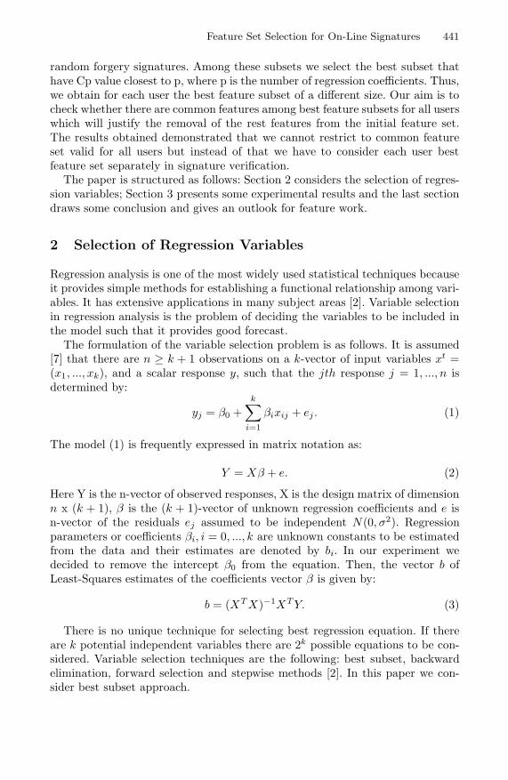
Feature Set Selection for On-Line Signatures 441
random forgery signatures. Among these subsets we select the best subset thathave Cp value closest to p, where p is the number of regression coefficients. Thus,we obtain for each user the best feature subset of a different size. Our aim is tocheck whether there are common features among best feature subsets for all userswhich will justify the removal of the rest features from the initial feature set.The results obtained demonstrated that we cannot restrict to common featureset valid for all users but instead of that we have to consider each user bestfeature set separately in signature verification.
The paper is structured as follows: Section 2 considers the selection of regres-sion variables; Section 3 presents some experimental results and the last sectiondraws some conclusion and gives an outlook for feature work.
2 Selection of Regression Variables
Regression analysis is one of the most widely used statistical techniques becauseit provides simple methods for establishing a functional relationship among vari-ables. It has extensive applications in many subject areas [2]. Variable selectionin regression analysis is the problem of deciding the variables to be included inthe model such that it provides good forecast.
The formulation of the variable selection problem is as follows. It is assumed[7] that there are n ≥ k + 1 observations on a k-vector of input variables xt =(x1, ..., xk), and a scalar response y, such that the jth response j = 1, ..., n isdetermined by:
yj = β0 +k∑
i=1
βixij + ej . (1)
The model (1) is frequently expressed in matrix notation as:
Y = Xβ + e. (2)
Here Y is the n-vector of observed responses, X is the design matrix of dimensionn x (k + 1), β is the (k + 1)-vector of unknown regression coefficients and e isn-vector of the residuals ej assumed to be independent N(0, σ2). Regressionparameters or coefficients βi, i = 0, ..., k are unknown constants to be estimatedfrom the data and their estimates are denoted by bi. In our experiment wedecided to remove the intercept β0 from the equation. Then, the vector b ofLeast-Squares estimates of the coefficients vector β is given by:
b = (XT X)−1XTY. (3)
There is no unique technique for selecting best regression equation. If thereare k potential independent variables there are 2k possible equations to be con-sidered. Variable selection techniques are the following: best subset, backwardelimination, forward selection and stepwise methods [2]. In this paper we con-sider best subset approach.

442 D. Boyadzieva and G. Gluhchev
A number of criteria have been proposed for selecting the best subset orsubsets of independent variables in linear regression analysis. Mallows proposedCp as a criterion to decide on suitable subset among contending subsets. It is ameasure of the standardized total squared error defined as:
Cp =RSSp
σ2− (n − 2p). (4)
In this equation RSSp denotes residual sum of squares for the particularregression with p variables including the intercept, if any. σ2 is an estimate ofresidual mean square σ2 for full regression:
σ2 =1
n − k
n∑
j=1
(yj −k∑
i=1
βixij)2. (5)
If a model is adequate, i.e. does not suffer from lack of fit, then E(RSSp) =(n − p)σ2 and the following is true for that model:
E(Cp) ≈ p. (6)
This means that we expect Cp value to be about p. A plot of Cp versus pdisplays the adequate models as points close to the line Cp = p. Subsets withsmall values of Cp and values of Cp close to p are considered good.
Hocking and Leslie [5] further describe a method which allows thus subsetto be identified after consideration of only a small fraction of all
(kp
)possible
subsets of size p. LaMotte and Hocking [6] modified this algorithm in a way thatmoderately large problems can be treated with minimum of computation. Thealgorithm specifies the subset of size r to be deleted. In the following, the termsr-subset and p-subset will always refer, respectively, to subsets being deleted andsubsets being retained.
The method for selection of best subset is based on m-variable reductions, i.e.reductions in the regression sum of squares due to eliminating subsets of size mfrom the k-variable equation. Typically 1 ≤ m ≤ 4 and m = 1 in the originalmethod [5]. These m-variable reductions are used to determine the best r-subsetto be removed, for r > m. The reduction in the regression sum of squares dueto removing a set of r variables is given by:
Redr = RSSp − RSSk. (7)
The set of r variables for which this reduction is minimum specifies the subsetof size p (p = k − r) variables in the regression to be retained for which residualsum of squares is minimum. It is suggested in [5] that Cp statistic can also becomputed by using this reduction in the following way:
Cp =Redr
σ2− (2p − k). (8)

Feature Set Selection for On-Line Signatures 443
The steps of the generalized algorithm are as follows [6]: First, the k-variableequation is fitted with all variables present and the reductions in the regres-sion sum of squares, called univariate reduction, due to deleting each of thek-variables, are calculated. If a single variable, say ith is removed from the re-gression, its univariate reduction is given by:
Θi = σ2t2i . (9)
t2i =b2i
σ2bi
. (10)
The square of t-statistic associated with ith regression coefficient is denotedby t2i and the standard error of the estimated coefficient bi is denoted by σbi .The standard errors of the estimated coefficients are the square roots of thediagonal elements of the coefficient covariance matrix. After this, the variablesare relabeled according to the order of these univariate reductions. Having thevariables relabeled, the reductions in the regression sum of squares due to all ofthe
(km
)subsets of size m are evaluated. These are called m-variable reductions.
Each subset of size m is denoted by the subscripts of the variables in thatsubset in increasing order. That is, a m-subset is described as (i1, i2, ..., im)where 1 ≤ ij ≤ k and i1 ≤ i2 ≤ . . . ≤ im. Next these m-variable reductionsare ordered in increasing order of magnitude and are used to define stages forinspecting the r-subsets. Only those m-subsets whose first index is (r − m + 1) or greater are used to define a stage and hence we evaluate only them. Ther-subsets in a stage defined by an m-subset contain r indices consisting of thoseindices in the defining m-subset and r − m indices which are less than the firstindex in the m-subset. There are total of
(k−r+m
m
)stages defined in this way. The
stages are numbered according to the magnitude of the m-variable subset whichdefine them. Thus Stage 1 will consist of r-subsets defined by the m-subset withsmallest reduction.
In general, at the qth stage we evaluate the reductions due to all subsetsdefined in the qth stage and ask if the smallest reduction in the regression sumof squares computed for an r-subset obtained in all Stages before the qth stage(1, 2, . . . , q ) is less than the reduction due to the m-subset defining Stage (q+1).If so, we terminate having identified the best subset of size p obtained by thecorresponding r-subset and if not we proceed to Stage (q + 1).
3 Experiment
The database for our experiment contains 140 signatures collected from fourteenusers. All ten signatures of each user are acquired by using a digitizing tabletWacom Intuos3 A5 PTZ-630 having a resolution of 5080 lines per inch and anacquisition area of the pad of 152.4 x 210.6 mm and sampling rate of 200 pointsper second. Signature raw data is obtained using the .NET Tablet PC SDK 1.7in a C# software program. Having raw data, we evaluate all the features listedin Table 1.

444 D. Boyadzieva and G. Gluhchev
Table 1. Signature features
A1 height A2 height to widthratio
A3 number of points
A4 distance betweeninitial and centerpoint
A5 distancebetween end andcenter point
A6 angle of the linebetween centerand initial points
A7 angle of the linebetween centerand end points
A8 angle of the linebetween initialand end points
A9 distance betweenleftmost and cen-ter points
A10 angle of the linebetween centerand leftmostpoints
A11 angle of the linebetween centerand rightmostpoints
A12 distance betweenleftmost and ini-tial points
A13 distance betweenrightmost andend points
A14 angle of the lineangle of the linebetween leftmostand initial points
A15 angle of the linebetween end andrightmost points
The number of features is k = 15 and the number of signatures is n = 20 (tengenuine and ten random forgeries). For each user we construct a txt file. Each lineof that file contains signature features values separated by a semicolon followedby 1 (if genuine, i.e. first class) or -1 (if forgery, i.e. second class). The randomforgeries for a given users are just randomly selected signatures of the rest users.Our software program processes each of these fourteen files by performing themethod described in Section 2 and finds the best subset of size p (p = k − r)for variable values of r (3 < r < 13 ). Among these subsets we select the subsetthat have Cp value closest to p. These subsets for each user are listed in Table 2.
Table 2. Best p-subsets for each user
User No Size of p-subset Best p-subset
1 6 A2;A5;A7;A12;A13;A15
2 9 A3;A5;A6;A7;A8;A9;A10;A11;A12
3 11 A2;A4;A5;A6;A7;A8;A9;A10;A13;A14;A15
4 11 A1;A3;A4;A6;A7;A8;A9;A11;A12;A13;A15
5 5 A1;A2;A5;A9;A15
6 6 A4;A8;A9;A10;A12;A147 7 A1;A2;A5;A8;A11;A12;A13
8 9 A1;A2;A3;A4;A5;A8;A9;A10;A15
9 11 A2;A5;A6;A7;A8;A9;A11;A12;A13;A14;A15
10 8 A4;A6;A9;A10;A11;A12;A13;A14
11 9 A1;A3;A4;A5;A6;A7;A9;A11;A13
12 11 A1;A2;A3;A4;A5;A6;A7;A9;A10;A11;A15
13 10 A1;A2;A3;A5;A6;A8;A10;A11;A12;A14
14 10 A1;A2;A3;A4;A5;A7;A8;A9;A10;A11

Feature Set Selection for On-Line Signatures 445
These results demonstrate that the number of features is significantly reducedfor some users but there are not common features among best feature subsetsfor all users which will justify the removal of the rest features from the initialfeature set. That is because all the features have approximately equal numberof occurrences in best subsets. The results demonstrated that we cannot restrictto common feature set valid for all users but instead of that we have to considereach user best feature set separately in signature verification.
4 Conclusion
In this paper we present a method for feature set selection based on MallowsCp criterion for regression and conduct an experiment in order to test it with adatabase of 140 signatures from fourteen users. The obtained results demonstratethat this approach can be used for feature set reduction for a particular userbefore his/her signature verification. Probably the small number of features doesnot allow the presence of common features for all users. Therefore, the focus ofour future work will be the application of the method for selection of regressionvariables for larger feature set. Also, we will experiment with skilled signatureforgeries and investigate the problem further.
Acknowledgements
This work is supported by the European Social Fund and Bulgarian Ministryof Education, Youth and Science under Operative Program Human ResourcesDevelopment, Grant BG051PO001-3.3.04/40.
References
1. Nalwa, V.S., Ekeland, I.: Automatic on-line signature verification. Proceedings ofthe IEEE 85, 213–239 (1997)
2. Chatterjee, S., Hadi, A.: Regression Analysis by Example, 4th edn. New York (2006)3. Leclerc, F., Plamondon, R.: Automatic signature verification: the state of the art
1989-1993. International Journal of Pattern Recognition and Artificial Intelligence 8,643–660 (1994)
4. Richiardi, J., Ketabdar, H., Drygajlo, A.: Local and Global Feature Selection forOn-line Signature Verification. In: Eighth International Conference on DocumentAnalysis and Recognition (ICDAR 2005), pp. 625–629 (2005)
5. Hocking, R.R., Leslie, R.n.: Selection of the Best Subset in Regression Analysis.Technometrics 9, 531–540 (1967)
6. LaMotte, L.R., Hocking, R.R.: Computational Efficiency in the Selection of Regres-sion Variables. Technometrics 12, 83–93 (1970)
7. Hocking, R.R.: The Analysis and Selection of Variables in Linear Regression. Bio-metrics 32, 1–50 (1976)
8. Mallows, C.L.: Some Comments on Cp. Technometrics 15, 661–675 (1973)
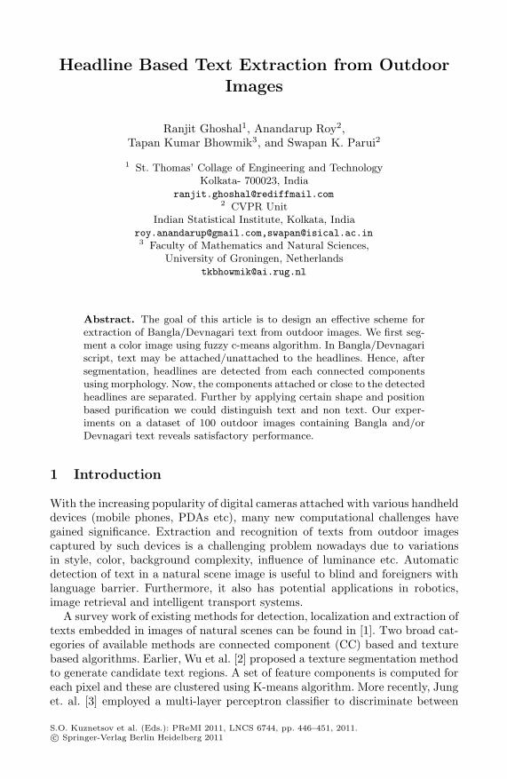
Headline Based Text Extraction from Outdoor
Images
Ranjit Ghoshal1, Anandarup Roy2,Tapan Kumar Bhowmik3, and Swapan K. Parui2
1 St. Thomas’ Collage of Engineering and TechnologyKolkata- 700023, India
[email protected] CVPR Unit
Indian Statistical Institute, Kolkata, [email protected],[email protected] Faculty of Mathematics and Natural Sciences,
University of Groningen, [email protected]
Abstract. The goal of this article is to design an effective scheme forextraction of Bangla/Devnagari text from outdoor images. We first seg-ment a color image using fuzzy c-means algorithm. In Bangla/Devnagariscript, text may be attached/unattached to the headlines. Hence, aftersegmentation, headlines are detected from each connected componentsusing morphology. Now, the components attached or close to the detectedheadlines are separated. Further by applying certain shape and positionbased purification we could distinguish text and non text. Our exper-iments on a dataset of 100 outdoor images containing Bangla and/orDevnagari text reveals satisfactory performance.
1 Introduction
With the increasing popularity of digital cameras attached with various handhelddevices (mobile phones, PDAs etc), many new computational challenges havegained significance. Extraction and recognition of texts from outdoor imagescaptured by such devices is a challenging problem nowadays due to variationsin style, color, background complexity, influence of luminance etc. Automaticdetection of text in a natural scene image is useful to blind and foreigners withlanguage barrier. Furthermore, it also has potential applications in robotics,image retrieval and intelligent transport systems.
A survey work of existing methods for detection, localization and extraction oftexts embedded in images of natural scenes can be found in [1]. Two broad cat-egories of available methods are connected component (CC) based and texturebased algorithms. Earlier, Wu et al. [2] proposed a texture segmentation methodto generate candidate text regions. A set of feature components is computed foreach pixel and these are clustered using K-means algorithm. More recently, Junget. al. [3] employed a multi-layer perceptron classifier to discriminate between
S.O. Kuznetsov et al. (Eds.): PReMI 2011, LNCS 6744, pp. 446–451, 2011.c© Springer-Verlag Berlin Heidelberg 2011

Headline Based Text Extraction from Outdoor Images 447
text and non-text pixels. Considering Bangla/Devnagari script, Bhattacharya et.al. [4] proposed a scheme based on analysis of CCs for extraction of Devnagariand Bangla texts from camera captured outdoor images. Also a few criteria forrobust filtering of text components have been proposed. Bangla and Devnagariare two most popular Indian scripts used by more than 200 and 500 millionpeople respectively in the Indian subcontinent. An unique and common charac-teristic of these two scripts is the existence of certain headlines that act as aninterlink among symbols of a word. We here, take an interest into color imagesembedding text. We first extract a number of color and shape based featuresfrom an input color image. The fuzzy c-means clustering is applied on thesefeatures, for segmentation (Sect. 2). After color image segmentation, headlinesare detected from each CCs using morphology on the skeleton image (Sect. 3).Afterwards, the CCs attached with these headlines are separated. These sepa-rated components may contain both text and non-text. We apply certain shapeand position based purification in order to distinguish between text and non text(Sect. 4). However some text portions, that are not connected with headline, willnot be separated by the above procedure. To cope this, we increase the area ofthe bounding box of each CC to a specified limit. The portions that lie inside thismodified bounding box are now studied against the previous criteria to obtaintext (Sect. 5).
Concerning the dataset, to the best known, no benchmark dataset of outdoorimages consisting Bangla and/or Devnagari is available. The present study isbased on a set of 100 outdoor images. Initial tests (Sect. 6) show well separationof texts from the images.
2 Color Image Segmentation
Color image segmentation is our first step of text extraction. The fuzzy c-meansalgorithm is used for color image segmentation. Before applying c-means, weextract some features from the normalized RGB image. Let us consider a pixel pi
of the image. Then pi can be described by the tuple (ri, gi, bi) i.e. the normalizedR, G and B values. Besides, these three color values, we take another shape basedfeature of pi. Inside an object (text here), intensity of pixels are assumed to behomogenous. We consider an n×n window surrounding pi. Let βi be the numberof pixels having same intensity as pi inside the n × n window. Then βi is ouranother feature. Combining, the feature vector (fi) corresponding to the pixel pi
is: fi = (ri, gi, bi, βi). These features are sent to the fuzzy c-means clusteringprocedure.
3 Morphology Based Headline Detection
Most of the Bangla and/or Devnagari characters are connected by the headline.Hence, in order to extract the Bangla and/or Devnagari text portions we shoulddetect the headline that joins them. Here, we apply mathematical morphologyoperation to obtain the lines inside the image. Further, applying some filtering

448 R. Ghoshal et al.
we are able to detect the headline. The procedure works as follows. At first suf-ficiently small and large CCs are removed. For each remaining CCs, the skeletonimage is constructed by morphological operation. Let us denote the skeletonimage by A. With the skeleton image, we perform morphological opening oper-ation to extract straight lines. It is evident that opening of an image A with alinear structuring element B can effectively identify the horizontal line segmentspresent in a CC. However, a suitable choice of the length of this structuringelement is crucial for processing at the latter stages and we empirically set thislength as 21 pixels for the present dataset. The effect of skeletonisation removespixels on the boundaries of the image but does not allow components to breakapart. After skeletonisation, only the required pixels remain and thus a less num-ber of lines detected. However, if no such lines are detected, we need to applymorphology on the original CC. Also, we may encounter a component smallenough that we could not find any horizontal line. Such components remain asit is.
Now we have a set of lines over the image. We next apply some simple criteriato separate out possible headlines. Let a detected line be denoted by Li. LetHu and Hl be the heights of the portions of the corresponding CCs lie at theupper and at the lower half of the line Li. Bangla characters mostly lie at thelower portion of the headline, only a small portion may reside at the upper ofthe headline. So, for a headline Li we should have Hu < Hl. Thus at the nextstep we sort out all the lines Li for which Hu < Hl. These lines mostly representthe headlines.
4 Headline Attached Text Portion Separation
After finding the headlines, the components attached with these headlines areseparated. These components may include text as well as non-text. However,applying some text specific conditions we are able to separate out text compo-nents. These conditions are described below. All the concerned components aresubjected to these conditions in the same sequence as given. One important notehere, is, the thresholds specified in one condition are found after performing theprevious conditions. Thresholds may differ if the sequence is altered.
1. Removal of boundary attached connected components: Generally, text likepatterns are not attached with boundary of the image. So, we first removeall boundary attached CCs using morphological reconstruction.
2. Elongatedness ratio: For elongatedness ratio (ER) we use the measure de-signed by Roy et. al. [5]. Empirically it is found that a component with ERvalue greater than 5 is a text part.
3. Number of holes: Usually, text like patterns contain less number of holesthan non-text patterns. Using the Euler number, we calculate the numberof holes inside a component. Found empirically, a text component has lessthan 9 holes.
4. Aspect ratio: The aspect ratio of a non-text component is either very smallor very large. We found by experiments, that the aspect ratio of a textcomponent becomes less than 0.3 or greater than 2.0.
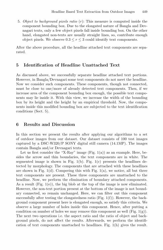
Headline Based Text Extraction from Outdoor Images 449
5. Object to background pixels ratio (r): This measure is computed inside thecomponent bounding box. Due to the elongated nature of Bangla and Dev-nagari texts, only a few object pixels fall inside bounding box. On the otherhand, elongated non-texts are usually straight lines, so, contribute enoughobject pixels. We observe 0.3 ≤ r ≤ 3 could identify text components.
After the above procedure, all the headline attached text components are sepa-rated.
5 Identification of Headline Unattached Text
As discussed above, we successfully separate headline attached text portions.However, in Bangla/Devnagari some text components do not meet the headline.Now we consider such components. These components, though not connected,must be close to one/more of already detected text components. Then, if weincrease area of the component bounding box enough, the possible text compo-nents may lie inside it. With this view, we increase the width of the boundingbox by its height and the height by an empirical threshold. Now, the compo-nents inside this modified bounding box are subjected to the text identificationconditions (Sect. 5).
6 Results and Discussion
In this section we present the results after applying our algorithms to a setof outdoor images from our dataset. Our dataset consists of 100 test imagescaptured by a DSC-W320/P SONY digital still camera (14.1MP). The imagescontain Bangla and/or Devnagari texts.
Let us first consider the “X-Ray” image (Fig. 1(a)) as an example. Here, be-sides the arrow and thin boundaries, the text components are in white. Thesegmented image is shown in Fig. 1(b). Fig. 1(c) presents the headlines de-tected by morphology. The components that are attached with these headlinesare shown in Fig. 1(d). Compering this with Fig. 1(a), we notice, all but threetext components are present. These three components are unattached to theheadline. Now, we perform the elimination of boundary attached components.As a result (Fig. 1(e)), the big blob at the top of the image is now eliminated.However, the non-text portion present at the bottom of the image is not bound-ary connected, so remain unchanged. Here, we can filter out this componentsuccessfully after testing the elongatedness ratio (Fig. 1(f)). However, the back-ground component present here is elongated enough, so satisfy this criteria. Weobserve a large number of holes inside this component. Hence, after putting acondition on number of holes we may remove this component as well (Fig. 1(g)).The next two operations i.e. the aspect ratio and the ratio of object and back-ground pixels, do not affect the results. Afterwards, we perform the identifi-cation of text components unattached to headlines. Fig. 1(h) gives the result.
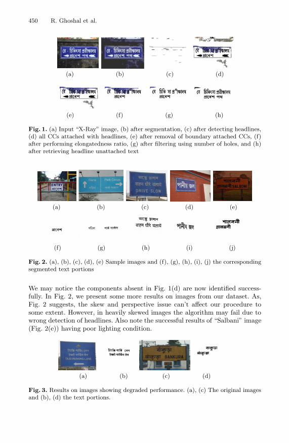
450 R. Ghoshal et al.
(a) (b) (c) (d)
(e) (f) (g) (h)
Fig. 1. (a) Input “X-Ray” image, (b) after segmentation, (c) after detecting headlines,(d) all CCs attached with headlines, (e) after removal of boundary attached CCs, (f)after performing elongatedness ratio, (g) after filtering using number of holes, and (h)after retrieving headline unattached text
(a) (b) (c) (d) (e)
(f) (g) (h) (i) (j)
Fig. 2. (a), (b), (c), (d), (e) Sample images and (f), (g), (h), (i), (j) the correspondingsegmented text portions
We may notice the components absent in Fig. 1(d) are now identified success-fully. In Fig. 2, we present some more results on images from our dataset. As,Fig. 2 suggests, the skew and perspective issue can’t affect our procedure tosome extent. However, in heavily skewed images the algorithm may fail due towrong detection of headlines. Also note the successful results of “Salbani” image(Fig. 2(e)) having poor lighting condition.
(a) (b) (c) (d)
Fig. 3. Results on images showing degraded performance. (a), (c) The original imagesand (b), (d) the text portions.

Headline Based Text Extraction from Outdoor Images 451
Table 1. The precision and recall computation for our dataset
No. ofStatus
Total Correctly WronglyPrecision Recall
Images text recognized text recognized text
62 Perfectly extracted 307 307 27 91.91% 100.00%
32Partially/extracted
147 91 29 75.83% 61.90%with some non text
06 Poor performance 27 09 31 22.50% 33.33%
100 481 407 87 82.38% 84.61%
The images in Fig. 3 show poor performance. The two images have headlineunattached text portions that are not restored. The precision and recall valuesof our algorithm obtained on the basis of the present set of 100 images arerespectively 82.38% and 84.61%. Detailed results are presented in Table 1.
7 Conclusion
This article provides a methodology that aids automatic extraction of visual textentities embedded in complex outdoor images. The proposed method is not verysensitive to image color, text font, skewness and perspective effects. Moreoverit analyzes only headline attached CC adding a few CC which are closed tothe headline. So, it becomes computationally efficient for real applications. Thismethod can be extended to scanned documents also. The results shown aresignificant based on a laboratory made dataset. In future, we shall study the useof machine learning tools to improve the performance.
References
1. Liang, J., Doermann, D., Li, H.: Camera based analysis of text and documents: asurvey. Int. Journ. on Doc. Anal. and Recog (IJDAR) 7, 84–104 (2005)
2. Wu, V., Manmatha, R., Riseman, E.M.: Textfinder: An automatic system to de-tect and recognize text in images. IEEE Trans. on Pattern Analysis and MachineIntelligence 21, 1224–1229 (1999)
3. Jung, K., Kim, I.K., Kurata, T., Kourogi, M., Han, H.J.: Text scanner with textdetection technology on image sequences. In: Proc. of Int. Conf. on Pattern Recog-nition, vol. 3, pp. 473–476 (2002)
4. Bhattacharya, U., Parui, S.K., Mondal, S.: Devanagari and bangla text extractionfrom natural scene images. In: Proc. of the Int. Conf. on Document Analysis andRecognition, pp. 171–175 (2009)
5. Roy, A., Parui, S.K., Paul, A., Roy, U.: A color based image segmentation andits application to text segmentation. In: Proc. of Ind. Conf. on Computer Vision,Graphics & Image Processing, pp. 313–319 (2008)

Incremental Methods in Collaborative Filtering
for Ordinal Data
Elena Polezhaeva
Lomonosov Moscow State University, Moscowlena [email protected]
Abstract. In modern collaborative filtering applications initial data aretypically very large (holding millions of users and items) and come in realtime. In this case only incremental algorithms are practically efficient.In this paper a new algorithm based on the symbiosis of IncrementalSingular Value Decomposition (ISVD) and Generalized Hebbian Algo-rithm (GHA) is proposed. The algorithm does not require to store theinitial data matrix and effectively updates user/item profiles when a newuser or a new item appears or a matrix cell is modified. The results ofexperiments show how root mean square error (RMSE) depends on thenumber of algorithm’s iterations and data amount.
Keywords: Collaborative filtering, singular value decomposition, Gen-eralized Hebbian algorithm, sparse matrix, large data, ordinal data, in-cremental data.
1 Introduction
Collaborative Filtering (CF) is used in recommender systems and CustomerRelationship Management System (CRM) for personalization. Initial data arerepresented by a sparse matrix Y = (yur)n×d, in which rows correspond ton users, columns — to d items (documents, films, etc.). Each matrix cell containsinformation about the usage of an item by a user. So matrix cell may be a rating,a sum paid by user, a mark about visiting site (0 or 1), etc.
The aim is to predict for any user his preferences towards items or, in otherwords, to fill any empty cell in the initial matrix.
The thin singular value decomposition (SVD) [1] is effective because it usesa compressed representation of the data. Reduced data (profiles) are formed forusers and items, then not all data are held. In modern collaborative filteringapplications initial data are typically very large (holding millions of users anditems), sparse and come in real time. So the requirement of incrementality isvery important. It should be possible to update stored data is case of appearingof a new user/item(1) or a new value in a matrix cell(2). Usually it is proposedto solve only one of these incremental problems. In works of Brand [1] new itemsand ratings are added efficiently. In paper [2] algorithm efficiently incorporatesinto the model new users or new ratings but doesn’t handle the addition of newitems.
S.O. Kuznetsov et al. (Eds.): PReMI 2011, LNCS 6744, pp. 452–457, 2011.c© Springer-Verlag Berlin Heidelberg 2011
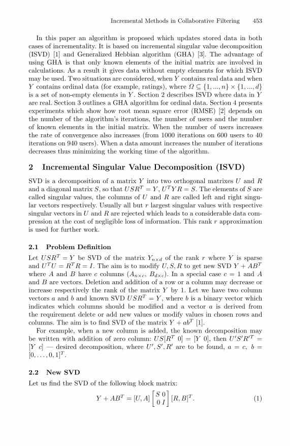
Incremental Methods in Collaborative Filtering 453
In this paper an algorithm is proposed which updates stored data in bothcases of incrementality. It is based on incremental singular value decomposition(ISVD) [1] and Generalized Hebbian algorithm (GHA) [3]. The advantage ofusing GHA is that only known elements of the initial matrix are involved incalculations. As a result it gives data without empty elements for which ISVDmay be used. Two situations are considered, when Y contains real data and whenY contains ordinal data (for example, ratings), where Ω ⊆ 1, ..., n × 1, ..., dis a set of non-empty elements in Y . Section 2 describes ISVD where data in Yare real. Section 3 outlines a GHA algorithm for ordinal data. Section 4 presentsexperiments which show how root mean square error (RMSE) [2] depends onthe number of the algorithm’s iterations, the number of users and the numberof known elements in the initial matrix. When the number of users increasesthe rate of convergence also increases (from 1000 iterations on 600 users to 40iterations on 940 users). When a data amount increases the number of iterationsdecreases thus minimizing the working time of the algorithm.
2 Incremental Singular Value Decomposition (ISVD)
SVD is a decomposition of a matrix Y into two orthogonal matrixes U and Rand a diagonal matrix S, so that USRT = Y , UT Y R = S. The elements of S arecalled singular values, the columns of U and R are called left and right singu-lar vectors respectively. Usually all but r largest singular values with respectivesingular vectors in U and R are rejected which leads to a considerable data com-pression at the cost of negligible loss of information. This rank r approximationis used for further work.
2.1 Problem Definition
Let USRT = Y be SVD of the matrix Yn×d of the rank r where Y is sparseand UT U = RT R = I. The aim is to modify U, S, R to get new SVD Y + ABT
where A and B have c columns (An×c, Bd×c). In a special case c = 1 and Aand B are vectors. Deletion and addition of a row or a column may decrease orincrease respectively the rank of the matrix Y by 1. Let we have two columnvectors a and b and known SVD USRT = Y , where b is a binary vector whichindicates which columns should be modified and a vector a is derived fromthe requirement delete or add new values or modify values in chosen rows andcolumns. The aim is to find SVD of the matrix Y + abT [1].
For example, when a new column is added, the known decomposition maybe written with addition of zero column: US[RT 0] = [Y 0], then U ′S ′R′T =[Y c] — desired decomposition, where U ′, S′, R′ are to be found, a = c, b =[0, . . . , 0, 1]T .
2.2 New SVD
Let us find the SVD of the following block matrix:
Y + ABT = [U, A][S 00 I
][R, B]T . (1)

454 E. Polezhaeva
Let P be an orthogonal basis of column space A = (I−UUT )A = A−UUTA.Then QR-decomposition is applied to A: A = PRA, where P is orthonormal, RA
is upper triangular, RA = PT (I − UUT )A. QR-decomposition of matrix [U, A]is:
[U, P ][I UT A0 RA
]= [U, A], (2)
which can be found from modified Gram–Schmidt orthogonalization [4].Similarly, let Q be an orthogonal basis of column space B − RRT B, then
QRB = (I − RRT )B where Q is orthonormal , RB is upper triangular, RB =QT (I − RRT )B.
Let us represent Y + ABT as a product of three matrixes:
Y + ABT = [U, P ][I UT A0 RA
] [S 00 I
] [I RT B0 RB
]T
[R, Q]T
= [U, P ]
([S 00 0
]+
[UT ARA
] [RT BRB
]T
︸ ︷︷ ︸K
)[R, Q]T ;
K =[S 00 0
]+
[(UT A)(BT R) (UT A)RT
B
RA(BT R) RARTB
].
Let U ′S′R′T be SVD of matrix K of rank (r + c). Making diagonalizationof K: U ′T KR′ = S′, new matrixes U ′, S′, R′ are formed. Then the modificationof SVD from rank r to rank (r + c) can be written as:
Y + ABT =([U P ]U ′)S ′([R Q]R′)T
. (3)
But instead of making operations with matrixes with big sizes new SVD ofY + ABT containing five matrixes is used:
Un×rU′r×rSr×rR
′Tr×rR
Tr×d, (4)
where UU ′, RR′, U, U ′ are orthonormal.If only one column or row are added following modifications are done: for
new SVD (a — n-dimensional vector, b — d-dimensional vector) modifiedGram–Schmidt orthogonalization is used:
z = UT a; p = a − Uz;
w = RT b; q = b − Rw;
Then K have simple representation and effective diagonalization may befound:
K =[S 00 0
]+
[zwT z‖q‖
‖p‖wT ‖p‖‖q‖]
.
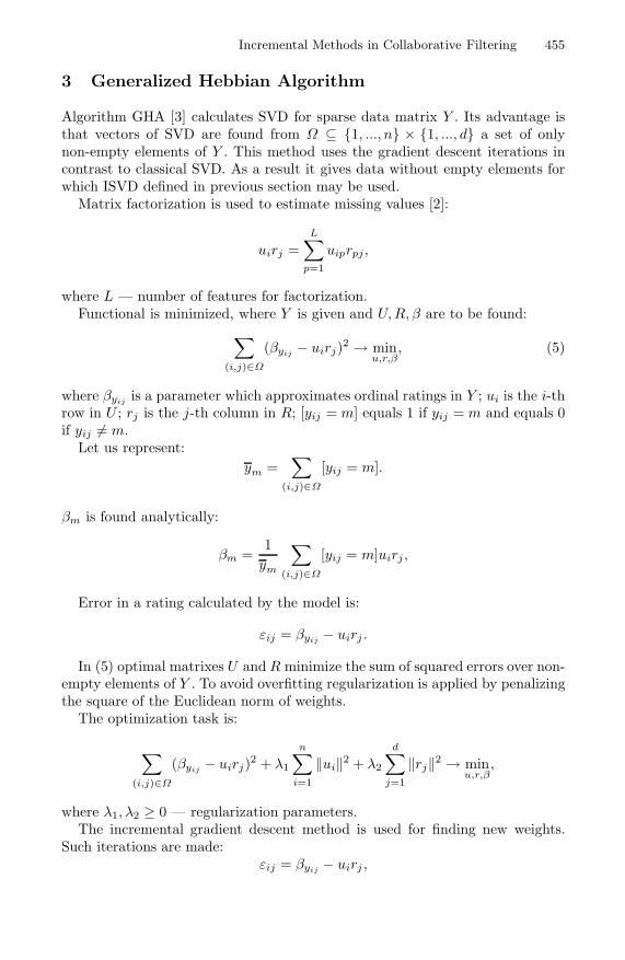
Incremental Methods in Collaborative Filtering 455
3 Generalized Hebbian Algorithm
Algorithm GHA [3] calculates SVD for sparse data matrix Y . Its advantage isthat vectors of SVD are found from Ω ⊆ 1, ..., n × 1, ..., d a set of onlynon-empty elements of Y . This method uses the gradient descent iterations incontrast to classical SVD. As a result it gives data without empty elements forwhich ISVD defined in previous section may be used.
Matrix factorization is used to estimate missing values [2]:
uirj =L∑
p=1
uiprpj ,
where L — number of features for factorization.Functional is minimized, where Y is given and U, R, β are to be found:
∑
(i,j)∈Ω
(βyij − uirj)2 → minu,r,β
, (5)
where βyij is a parameter which approximates ordinal ratings in Y ; ui is the i-throw in U ; rj is the j-th column in R; [yij = m] equals 1 if yij = m and equals 0if yij = m.
Let us represent:ym =
∑
(i,j)∈Ω
[yij = m].
βm is found analytically:
βm =1
ym
∑
(i,j)∈Ω
[yij = m]uirj ,
Error in a rating calculated by the model is:
εij = βyij − uirj .
In (5) optimal matrixes U and R minimize the sum of squared errors over non-empty elements of Y . To avoid overfitting regularization is applied by penalizingthe square of the Euclidean norm of weights.
The optimization task is:
∑
(i,j)∈Ω
(βyij − uirj)2 + λ1
n∑
i=1
‖ui‖2 + λ2
d∑
j=1
‖rj‖2 → minu,r,β
,
where λ1, λ2 ≥ 0 — regularization parameters.The incremental gradient descent method is used for finding new weights.
Such iterations are made:εij = βyij − uirj ,
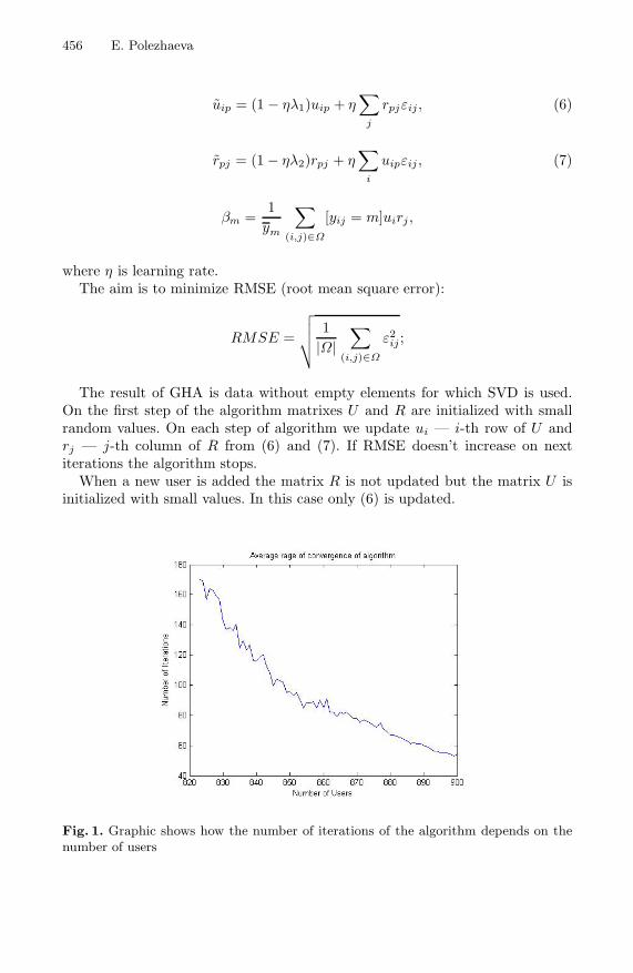
456 E. Polezhaeva
uip = (1 − ηλ1)uip + η∑
j
rpjεij , (6)
rpj = (1 − ηλ2)rpj + η∑
i
uipεij , (7)
βm =1
ym
∑
(i,j)∈Ω
[yij = m]uirj ,
where η is learning rate.The aim is to minimize RMSE (root mean square error):
RMSE =
√√√√ 1|Ω|
∑
(i,j)∈Ω
ε2ij ;
The result of GHA is data without empty elements for which SVD is used.On the first step of the algorithm matrixes U and R are initialized with smallrandom values. On each step of algorithm we update ui — i-th row of U andrj — j-th column of R from (6) and (7). If RMSE doesn’t increase on nextiterations the algorithm stops.
When a new user is added the matrix R is not updated but the matrix U isinitialized with small values. In this case only (6) is updated.
Fig. 1. Graphic shows how the number of iterations of the algorithm depends on thenumber of users

Incremental Methods in Collaborative Filtering 457
4 Experiments
Experiments were made on MovieLens data: 943 users, 1682 items, 100000 knownratings. Time factor and data amount have an effect on the rate of convergenceof the algorithm. The best results were achieved on rank-15 basis, η = 0.001and λ = 0.025: after 41 iterations RMSE = 0.923 . Brand in his work [5]achieved MAE = 0.7910 using only ISVD and rank-14 basis. It is very interestingthat all β ≥ 0 and they increase (even if we don’t impose conditions on β):β1 = 2.52; β2 = 3.03; β3 = 3.28; β4 = 3.63; β5 = 3.96. When the number of usersincreases the rate of convergence also increases (from 1000 iterations on 600 usersto 40 iterations on 940 users) (Fig.1). When a data amount increases the numberof iterations decreases thus minimizing the working time of the algorithm.
5 Results
The proposed method solves two incremental problems in CF and enables toupdate users’ and items’ profiles when new rows and columns are added andelements in Y are modified. Two tasks have been solved: when data are real orordinal. When a new user is added there is no need to retrain the entire model.Addition of a new item is a simple task in which a diagonalizable matrix iscalculated.
References
1. Brand, M.: Fast Low-rank modifications of the thin singular value decomposition.Linear Algebra and Its Applications 415(1), 20–30 (2006)
2. Takacs, G., Pilaszy, I., Nemeth, B., Tikk, D.: Scalable Collaborative Filtering Ap-proaches for Large Recommender Systems. The Journal of Machine Learning Re-search 10, 623–656 (2009)
3. Gorrell, G.: Generalized Hebbian Algorithm for Incremental Singular Value Decom-position in Natural Language Processing. In: Proceedings of EACL (2006)
4. Golub, G.: Matrix Computations, p. 728. Johns Hopkins University Press (1996)5. Brand, M.: Fast online SVD revisions for lightweight recommender systems. In:
SIAM International Conference on Data Mining (SDM) (2003)

A Scheme for Attentional Video Compression
Rupesh Gupta and Santanu Chaudhury
Dept. of EE, Indian Institute of Technology Delhi, New Delhi, [email protected], [email protected]
Abstract. In this paper an improved, macroblock (MB) level, visualsaliency algorithm, aimed at video compression, is presented. A Rel-evance Vector Machine (RVM) is trained over 3 dimensional featurevectors, pertaining to global, local and rarity measures of conspicu-ity, to yield probabalistic values which form the saliency map. Thesesaliency values are used for non-uniform bit-allocation over video frames.A video compression architecture for propagation of saliency values, sav-ing tremendous amount of computation, is also proposed.
1 Introduction
The acuity of the human eye is limited to only 1-2 of visual angle. This meansthat when viewed from a recommended distance of 1.2 m, the eye can crisplyperceive only a 2 cm radial region (computed as 1.2×tan(2/2)) on a standarddefinition 32 inch LCD. Also, a recent eye-tracking study [1] on inter-observersaliency variations in task-free viewing of natural images has concluded thatimages known to have salient regions generate highly correlated saliency maps fordifferent viewers. However, correctly estimating the points of human eye fixationstill remains a challenge. Itti et. al. [2] model visual attention as a combinationof low level features pertaining to the degree of dissimilarity between a regionand its surroundings. Novel center-surround approaches like [3] model saliency asthe fraction of dissimilar pixels in concentric annular regions around each pixel.Hou et. al. [4] take a completely different approach, suppressing the response tofrequently occurring features while capturing deviances. Other transform domainapproaches like [5,6] follow a similar line of thought. Although these approacheswork on psychological patterns with high accuracy, they often fail to detectsalient objects in real life images. Some failure cases of these approaches will beshown in our comparison results in Fig. 2.
The failure of these approaches can be attributed to Gestalts grouping prin-ciple which concerns the effect produced when the collective presence of a setof elements becomes more meaningful than their presence as separate elements.Thus, we model saliency as a combination of low level, as well as high level fea-tures which become important at the higher-level visual cortex. Many authorslike [7] resort to a linear combination of features such as contrast, skin color, etc.,but do not provide any explanation for the weights chosen. Hence, we proposea learning based feature integration algorithm where we train an RVM with 3dimensional feature vectors to output probabalistic saliency values.
S.O. Kuznetsov et al. (Eds.): PReMI 2011, LNCS 6744, pp. 458–465, 2011.c© Springer-Verlag Berlin Heidelberg 2011

A Scheme for Attentional Video Compression 459
One of the earliest automated (as opposed to gaze contingent), visual saliencybased, video compression model was proposed by Itti in [8]. In [8] a small num-ber of virtual foveas attempt to track the salient objects, over the video frames;and the non-salient regions are Gaussian blurred to achieve compression. Guo et.al. [5] use their PQFT approach for proto-object detection, and apply a multi-resolution wavelet domain foveation filter suppressing coefficients correspond-ing to background. Selective blurring can however lead to unpleasing artifactsand generally scores low on subjective evaluation. A novel bit allocation model,achieving compression while preserving visual quality is presented in [9] which weadopt here. In all these compression approaches, the saliency map is computedfor each frame which is avoidable considering the inherent temporal redundancyin videos. We propose here a video coding architecture, incorporating visualsaliency propagation, to save on a large amount of saliency computation, andhence time. This architecture is most effective for natural video sequences.
The rest of this paper is organized as follows. In Sect. 2, we describe the stepsfor computing the saliency map. Since all video coding operations are MB based,we learn saliency at MB level to save on unnecessary computation. Section 3describes a video coding architecture in which various issues relating to saliencypropagation/ re-calculation and bit allocation are addressed. We conclude withsome conclusions and directions for future research in Sect. 4
2 Generation of Saliency Map
We use color spatial variance, center-surround multi scale ratio of dissimilar-ity and pulse DCT to construct 3 feature maps. Then, a soft, learning basedapproach is used to arrive at the final saliency map.
2.1 Global Conspicuity: Color Spatial Variance
The lesser a particular color is globally present in a frame, the more it is likelyto catch the viewers attention. However, a color sparsely distributed over theentire frame need not be conspicuous owing to Gestalts principles. Hence, spatialvariance of colors can be employed as a measure of global conspicuity. We followthe method given in [10], based on representation of color clusters by Gaussianmixture models to calculate their spatial variance, to get this feature map. Thefeature map is normalized to the range [0,1]
2.2 Local Conspicuity: Multi-scale Ratio of Dissimilarity
The ‘pop-out’ effect has, since long [2], been attributed to the degree of dissim-ilarity between a stimulus and its surroundings. A simple method to accuratelycapture local saliency has been recently proposed in [3]. In this method, a multi-scale filter is designed to simulate the visual field. A summation of the fractionof dissimilar pixels in concentric ring-like regions around each pixel gives a mea-sure of conspicuity. We use this method to construct our second feature map.

460 R. Gupta and S. Chaudhury
However, this approach is slow, since a large number of computations and com-parisons are carried out for every pixel. Noting that background pixels generallyhave very low values of saliency, computation of saliency for these pixels is su-perfluous. Hence, we first run a SIFT algorithm and locate the keypoints in theimage, which are salient not only spatially but also across different scales. Wetake one keypoint at a time and compute its saliency using [3]. If the saliency ofthis point is above a threshold (0.4 here, required since a keypoint may lie on acluttered background), we start growing a region from that point. The saliencyvalue of neighboring pixels is used as region membership criterion and all pixelsvisited are marked so that they are not re-visited when a different seed pointis chosen. We stop when the distance between the new pixel and region meanexceeds a threshold (0.2 here). This feature map is also normalized to [0,1].
2.3 Rarity Conspicuity: Pulse Discrete Cosine Transform
A biologically plausible, real time model simulating lateral inhibition in thereceptive field has been proposed in [6]. It has also been shown to outperformother transform domain approaches like [5] both in terms of speed as well asaccuracy over psychological patterns. We apply the pulse DCT algorithm tosmoothened images to produce our rarity feature map. A Gaussian blurred imagesimulates the scene viewed from a distance and thus finer edge details in acluttered background are not noticed, leading to a sparser feature map. Wenormalize it to the range [0,1].
2.4 Learning to Integrate the Feature Maps
The steps followed for combining the 3 feature maps are as follows. First, weselected 30 images, of size 300×400, encompassing the failure cases of each ofthe 3 feature maps. 5 viewers were asked to mark each part of the image theyconsidered salient. In accordance with [1], our images (mostly taken from [10])had well-defined salient regions and hence the markings turned out to be exactlythe same for almost all images. Then, an MB level, 3 dimensional training data(total 450×30 points) was prepared taking average values of each of the 3 featuremaps over each MB of size 16×16. A target class label ’1’ was assigned to an MBif more than half of the pixels of that MB were marked salient; else class label’0’ was assigned. Next, we trained an RVM over this training data as a binaryclassification problem. Here we must point out that we are not really interestedin a binary label (salient/non-salient) but the relative saliency value of each MBwhich will later be used for bit allocation. A potential advantage of RVM overSVM, which is desired here, is that it provides posterior probabilities. Also, RVMhas better generalization ability and its sparser kernel function leads to fasterdecisions. The probabilistic outputs of the RVM formed our final saliency map.
To test the machine, we generated a testing data from 120 images (450×120points) and evaluated the saliency maps obtained against ground truth. Variousauthors like Bruce et. al. [11] have used area under the ROC curves to quantifythe quality of their algorithms. The ROC curve obtained on our own ground

A Scheme for Attentional Video Compression 461
truth data is shown in Fig. 1. Also shown in the same figure is a comparison ofour result with another leading graph based visual saliency approach [12], whichhas been shown to outperform various other approaches like [2]. We obtaineda 0.90048 (s.e. 0.00136) area under the curve compared to 0.87009 (s.e. 00161)for [12]. In the context of application of saliency to video compression, an FN(actually salient but classified non-salient) is costlier compared to an FP. Avery low FN rate, less than 2%, at the cut-off point reflects the potential of ouralgorithm for such applications. Some results and comparisons with [12] and [11]are shown in Fig. 2. A comparison with [3] and [6] is inherent in these results asour local and rarity feature maps respectively. It is apparent that our approachis better or at least at par with these other high-ranking approaches.
Fig. 1. ROC curves for our approach and [12] obtained by varying thresholds onsaliency values
Fig. 2. (a) Input image, (b) global, (c) local [3], (d) rarity [6] feature maps, (e) ourresized saliency map, (f) saliency map obtained from [12] and (g) [11]
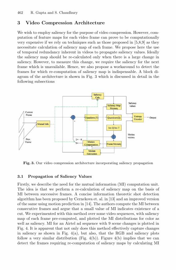
462 R. Gupta and S. Chaudhury
3 Video Compression Architecture
We wish to employ saliency for the purpose of video compression. However, com-putation of feature maps for each video frame can prove to be computationallyvery expensive if we rely on techniques such as those proposed in [5,8,9] as theynecessitate calculation of saliency map of each frame. We propose here the useof temporal redundancy inherent in videos to propagate saliency values. Ideallythe saliency map should be re-calculated only when there is a large change insaliency. However, to measure this change, we require the saliency for the nextframe which is unavailable. Hence, we also propose a workaround to detect theframes for which re-computation of saliency map is indispensable. A block di-agram of the architecture is shown in Fig. 3 which is discussed in detail in thefollowing subsections
Fig. 3. Our video compression architecture incorporating saliency propagation
3.1 Propagation of Saliency Values
Firstly, we describe the need for the mutual information (MI) computation unit.The idea is that we perform a re-calculation of saliency map on the basis ofMI between successive frames. A concise information theoretic shot detectionalgorithm has been proposed by Cernekova et. al. in [13] and an improved versionof the same using motion prediction in [14]. The authors compute the MI betweenconsecutive frames and argue that a small value of MI indicates existence of acut. We experimented with this method over some video sequences, with saliencymap of each frame pre-computed, and plotted the MI distributions for color aswell as saliency. MI for an Airtel ad sequence with 9 scene changes is plotted inFig. 4. It is apparent that not only does this method effectively capture changesin saliency as shown in Fig. 4(a), but also, that the RGB and saliency plotsfollow a very similar distribution (Fig. 4(b)). Figure 4(b) implies that we candetect the frames requiring re-computation of saliency maps by calculating MI

A Scheme for Attentional Video Compression 463
over the color channels. The frame where a large change is detected should becoded as an I frame (or I MBs in H.264) and saliency re-computed for this frameand stored. The method has been found to work best on natural video sequences.
Fig. 4. (a) MI plot for saliency maps, (b) MI plots of RGB and saliency overlaid. AnAirtel ad sequence with 9 cuts is used here.
For P frames, we make use of motion vectors to approximate saliency values.We select an MB in the current frame and look for the best match in the referenceframe. This best match may or may not exactly overlap an MB in the referenceframe, but we have the saliency values for only non overlapping 16×16 MBs.Therefore, we take a weighted average of the saliency values of each of the MBsunder the best match region the in reference frame, as the saliency value for theMB in current frame. The weights correspond to the amount of area overlap asshown in Fig. 5
Fig. 5. Image illustrating a weighted averaging of saliency values, the orange, blue,yellow, green colors denote the amount of overlap and hence weights
464 R. Gupta and S. Chaudhury
3.2 Selection of Quantization Parameters
Once the saliency map is obtained, bits may be non-uniformly distributed acrossa frame. We require a function which can optimally tune the quantization pa-rameters of salient and non-salient MBs to achieve compression, i.e, reduce rate(R), without any significant loss of perceptual quality, i.e, constant distortion(D). In [9], this is posed as a global optimization problem and solved using themethod of Lagrange multipliers. The final result for quantization step Qistep forthe ith MB having a saliency value wi is given as:
Qistep =Ws
wiSQstep . (1)
where W is the sum of saliency values over all MBs, s is the area of MBi (16×16here), S is the area of entire frame and Qstep is a fixed value depending onthe amount of distortion tolerable. This formula implies that the quantizationstep size should be inversely proportional to the saliency value which is com-pletely justified. We present here a short verification of how this formulationachieves compression without compromising on perceptual quality. Assuming aR-D function [15] for an MBi is given by:
Di = σ2i e−γRi or Ri =
1γ
log
(σ2
i
Di
). (2)
where σ2i is variance of encoding signal and γ is a constant coefficient. Ignoring
the constant term γ and taking σ2i = 1/α we get:
Ri = log
(1
αDi
). (3)
Now, the average rate R is calculated as∑N
i=1 sRi/S, where N is the number ofMBs. Noting that Di ∝ Qistep, we get after replacing Qistep by (1):
R =Ns
S
[log
(1
αQstep
)+ log
((w1.w2...wN )
1N
w1 + w2 + ... + wN
)+ log
(S
s
)]. (4)
From the above equation it is clear that the first term denotes the rate if everyMB was quantized with the same parameter Qstep, the second term is always ≤ 0by the AM-GM inequality and the third term is a constant. Thus R is reduced.It can also be readily observed from (1) that overall D (
∑wiDi/W ) remains
constant. We limit the Qistep to minimum and maximum values of max(0.5 ×Qstep, Qistep) and min(1.5 × Qstep, Qistep) respectively. Also, we smoothen oursaliency map using a Gaussian filter before computing the quantization step.This serves two purposes, firstly, it ensures that the salient object/region iscovered completely and secondly, it ensures a smooth transition from salient tonon-salient regions.

A Scheme for Attentional Video Compression 465
4 Conclusion
A vast amount of research has gone into modelling of the human visual systemwith each model having its own merits and shortcomings. The potential whichlies in an integration of these models has been demonstrated by the accuracy ofour results. A simple and effective learning based approach for such a unificationhas been presented. Though we make use of only 3 features, this model is easilyextendible to more features if desired. We computed saliency at MB level tosave computation, however our model is equally applicable at pixel level. Thecompression framework proposed, to approximate saliency of P frames, can savea lot of computation, speeding-up compression. We plan to integrate our it intothe H.264 coding system which remains a challenge owing to the complex modedecision metrics and hybrid coding structures in this standard [16].
References
1. Engelke, U., Maeder, A., Zepernick, H.J.: Analysing Inter-observer Saliency Vari-ations in Task-Free Viewing of Natural Images. In: ICIP, pp. 1085–1088 (2010)
2. Itti, L., Koch, C., Niebur, E.: A Model of Saliency-Based Visual Attention forRapid Scene Analysis. IEEE Trans. PAMI 20(11), 1254–1259 (1998)
3. Huang, R., Sang, N., Liu, L., Tang, Q.: Saliency Based on Multi-scale Ratio ofDissimilarity. In: ICPR, pp. 13–16 (2010)
4. Hou, X., Zhang, L.: Saliency Detection: A Spectral Residual Approach. In: CVPR,pp. 1–8 (2007)
5. Guo, C., Zhang, L.: A Novel Multiresolution Spatiotemporal Saliency DetectionModel and Its Applications in Image and Video Compression. IEEE Trans. ImageProc. 19(1), 185–198 (2010)
6. Yu, Y., Wang, B., Zhang, L.: Pulse Discrete Cosine Transform for Saliency-BasedVisual Attention. In: ICDL, pp. 1–6 (2009)
7. Chiang, J., Hsieh, C., Chang, G., Jou, F., Lie, W.: Region-of-Interest Based RateControl Scheme with Flexible Quality on Demand. In: ICME, pp. 238–242 (2010)
8. Itti, L.: Automatic Foveation for Video Compression Using a Neurobiological Modelof Visual Attention. IEEE Trans. Image Proc. 13(10), 1304–1318 (2004)
9. Li, Z., Qin, S., Itti, L.: Visual Attention Guided Bit Allocation in Video Compres-sion. Image and Vision Computing 29(1), 1–14 (2011)
10. Liu, T., Sun, J., Zheng, N.-N., Tang, X., Shum, H.-Y.: Learning to Detect a SalientObject. In: CVPR, pp. 1–8 (2007)
11. Bruce, N.D.B., Tsotsos, J.K.: Saliency Based on Information Maximization. In:NIPS, pp. 155–162 (2006)
12. Harel, J., Koch, C., Perona, P.: Graph-Based Visual Saliency. In: NIPS, pp. 545–552 (2006)
13. Cernekova, Z., Pitas, I., Nikou, C.: Information Theory-Based Shot Cut/Fade De-tection and Video Summarization. IEEE Trans. CSVT 16(1), 82–91 (2006)
14. Krulikovska, L., Pavlovic, J., Polec, J., Cernekova, Z.: Abrupt Cut Detection Basedon Mutual Information and Motion Prediction. In: ELMAR, pp. 89–92 (2010)
15. Bhaskaran, V., Konstantinides, K.: Image and Video Compression Standards: Al-gorithms and Architectures. Springer, Heidelberg (1997)
16. Chen, Z., Lin, W., Ngan, K.N.: Perceptual Video Coding: Challenges and Ap-proaches. In: ICME, pp. 784–789 (2010)
Using Conceptual Graphs for Text Mining in
Technical Support Services
Michael Bogatyrev and Alexey Kolosoff
Tula State University,Lenin ave. 92, 300600 Tula, Russia
[email protected], [email protected]
Abstract. Text mining problems of natural text classification and factextraction are important in developing information systems for TechnicalSupport Services. An approach which is based on joining acquisition ofconceptual graphs and keywords search technique is presented to theirsolution. Conceptual graphs have been created from e-mail queries sentto Technical Support Service. Correct conceptual graphs acquired from e-mail texts represent facts and situations which become patterns to searchin systems resources to resolve users problems. Experimental results ofimplementing proposed approach are presented.
Keywords: natural language texts classification, conceptual graphs,correctness of conceptual graphs, technical support services.
1 Introduction
Text mining strategies share many techniques such as machine learning, naturallanguage processing, text categorization, clustering, filtering, etc. These tech-niques can be classified as ones which use texts words and others which usesemantic models constructed from text. Two known strategies, Latent Seman-tic Analysis (LSA) [1] and Formal Concept Analysis (FCA) [2] illustrate thatdifference. LSA uses term-document matrices which describe the occurrences ofterms in textual documents and has been created from documents words. FCAuses conceptual models - conceptual graphs [3] and conceptual structures (for-mal concept lattices) which are formal models. The mentioned strategies alsohave different mathematical nature: LSA is founded on geometry and statisticswhereas FCA is founded on logic and algebra (the lattice theory).
Traditionally only one approach, based on keywords or formal models, is ap-plied in industrial text mining systems. Nevertheless modern problems of textualanalysis may have significant complexity and it becomes necessary to apply hy-brid approaches to solve them.
In our work namely that complex problem is investigated. As the result wedecided to apply keywords technique and conceptual graphs in our Text Miningsystem. Although each separate technique does not solve the problem, theircombination produces good preliminary results.
S.O. Kuznetsov et al. (Eds.): PReMI 2011, LNCS 6744, pp. 466–471, 2011.c© Springer-Verlag Berlin Heidelberg 2011

Using Conceptual Graphs for Text Mining in Technical Support Services 467
2 Problem Statement
Technical Support Services (TSS) have been intended to help users to solvespecific problems with a product - electronics, goods or software. Users sendqueries to TSS as natural language e-mail texts. It is needed to resolve queriesand to find an appropriate decision represented as help topics, useful URLs ore-mail reply. As a rule the system’s reply is prepared manually by support teamusing system’s resources as it is shown on Fig.1.
Questions &
Answers Database
Forums
Web Form
Self-Help Resources DB (Help, FAQ, How To, etc.)
Support Team
Search Engine
User queries:natural language
e-mail texts
System’s reply:Documents or URLs
Fig. 1. The structure of a Technical Support Service
When the number of queries significantly grows, automation of creating TSSreplies becomes very important. That automation is implemented in the TSSSearch Engine shown on Fig.1.
There are two basic text mining problems solved by the Search Engine. Thefirst one is the problem of natural text classification. The second is the problemof fact extraction. These problems have some peculiarities. The query text mustbe classified according to various resources of the TSS. TSS database containsdocumentation, help topics, e-mails of queries and replies. To find an appropriatedecision it is needed to refer to all these resources. The decision may exist asan example answer ready to be sent to a user or it can be constructed fromseparate pieces. Fact extraction problem is to find two kinds of objects in thequery texts: things which being analyzed text is about and situations which tookusers attention.
3 General Approach to Solution
Considering the problems of natural text classification and fact extraction de-scribed in the previous section, we propose the following general approach totheir solution:

468 M. Bogatyrev and A. Kolosoff
1. Having a flow of user e-mail queries we nevertheless do not apply classicalmachine learning technique because the style and contents of queries arevery individual. But it is worth to collect queries and corresponding repliesin the system’s database to apply them in further analysis. So, a kind ofself-learning is possible in the system.
2. Things and situations described in a query are represented by words andphrases. So we need to find keywords in the query text which correspondto terms described in system’s database texts. Since learning technique isimpossible in the system, another way of keywords extraction is needed. Textfiltering is standard and evidently necessary technique for e-mail texts innatural language. We apply term filtering to find direct terms correspondingto the terms described in systems database texts. For example, the driverword in a query in the software TSS has high probability to be the term. So atext containing this word can be classified as referring to the topic ”Drivers”in the system’s database texts. To implement term filtering a thesaurus asan additional resource must be created in the system.
3. Text filtering is not exhaustive technique for classification. Besides terms, aquery text contains many words which can also be useful for analysis. Thepersonal style of an author has certain representation in query text as a setof specific words and language grammar distortions (slang). Nevertheless ouranalysis of real queries shows that the following heuristic principle is valid:despite the personal style, every author uses grammatically correct phraseswhen describes problematic situations. Therefore semantics of these gram-matically correct phrases in a query text may represent useful informationabout situations we need to extract. We apply conceptual graphs for mod-elling semantics of sentences or phrases of the text and use their conceptsand relations for further analysis.
Conceptual graphs acquisition from natural language texts is the problem whichhas no closed solution for arbitrary texts. We assume that the following circum-stances cause the success of creating conceptual graphs:
1. query texts are not long and all their sentences may be processed for acqui-sition in appropriate time;
2. grammatically correct phrases in the sentences produce correct conceptualgraphs possibly being sub graphs in incorrect conceptual graph of the wholesentence.
The following rough criterion of correctness of conceptual graph is admissiblehere: correct conceptual graph has no isolated concepts. An isolated concept is aconcept which has no connection to any relation.
4 System Implementation and Experimental Results
The TSS Text Mining system works according to the following stages.

Using Conceptual Graphs for Text Mining in Technical Support Services 469
1. Text documents indexing. All TSS documents have been indexed ac-cording to selected terms. These terms represent topics and main notes pre-sented in system documentation. Terms are either single words or severalwords phrases (no more than 4 words). Term weights are calculated via thewell-known tf-idf formula [4]. The TSS complex index is the only additionalmodification of TSS information resource realized in standard database tech-nology (MS SQL Server).
2. Conceptual graphs acquisition and processing. Conceptual graphs areapplied as an instrument of extracting keywords and key phrases accordingto the principle described below.
3. Search relevant documents in TSS database. Keywords and keyphrases corresponding to each e-mail text and extracted by conceptualgraphs processing have been used as queries for full-text search in TSS in-dexed database.
Consider the last two stages in some detail.
4.1 Conceptual Graphs Acquisition and Processing
We use our software [5] for conceptual graphs acquisition from natural languagetexts. The software is based on existing approaches of lexical, morphological andsemantic analysis. Semantic roles labeling [6] is applied as the main instrumentfor constructing relations in acquisition algorithm. The acquisition algorithmworks with our recently developed controllable grammatical templates. Usingthese templates, it is possible to adapt acquisition algorithm as to certain lan-guage grammar (Russian or English in the current version of the system) as tosome peculiarities of concrete language. User interface has also tools for recog-nizing incorrect conceptual graphs.
Conceptual graphs being acquired from all sentences of a query text are ap-plied to detect keywords and key phrases. As a rule, incorrect conceptual graphsindicate that there is no useful information in processed text. For example, con-ceptual graph acquired from the ”Thanks in advance” phrase, G1 = [advance:”][thank:”]1 is incorrect since it has no relation. TSS user can handle any acquiredgraph by using interface tools including visualization. That helps finding possiblyvalid keywords in incorrect conceptual graphs.
All acquired correct conceptual graphs considered as potential source of key-words and key phrases for the next search. Concepts connected with the agentrelation may represent terms and have been picked as keywords. Some termmay consist of several words, for example Remote Agent Service. The relationgenitive in its graph G2 = [remote*a:”] [service*b:”] [agent*c:”] (genitive?b?c)(attribute?c?a) indicates that Agent Service is the single whole. All graphshaving simple structure with genitive and attribute relations are considered assources of keywords and key phrases.
1 Here we use the CGIF format [3] for representing conceptual graphs.

470 M. Bogatyrev and A. Kolosoff
It is known that relations in conceptual graphs have linguistic meaning atfirst. But some of them can directly indicate a situation. That is the loca-tion relation and it is also considered as key phrases indicator. For example,it is illustrated by the phrase ”stop on error” and its conceptual graph G3 =[error*a:”][stop*b:”](location?b?a) .
4.2 Search Relevant Documents
All keywords and key phrases extracted by conceptual graphs processing are thentreated as queries for full-text search in TSS indexed database. For each e-mailtext they constitute a query vector. We devoted special attention to applyingLSA search strategy for such queries. We also compared it with other methodswhich use ranking functions of Okapi BM25 [7], SQL Server iFTS [8] and rankingfunction of Google. An experiment was conducted on the textual database withmore than 7000 help topics belonging to online help systems of three differentsoftware products. Employees of the products vendor company were asked torate (from 1 to 4) the quality of search results (including their ranking) fortop 10 most popular queries retrieved from the users queries statistics. A shortsummary is presented in the table below.
Table 1. Search results ratings for 10 most popular queries
Search Query LSA Okapi BM25 SQL Server iFTS Google
working with grids 3 1 4 4load testing 4 2 3 3web testing 4 3 2 3Remote Agent Service 4 2 2 4name mapping template 4 3 3 2stop on error 3 2 4 4object not found 3 4 4 3UI Automation Silverlight 4 4 4 3testing flash applications 4 4 3 4web service testing 4 4 3 4Total (max. 40): 37 29 32 34
Here Google refers to Google web search in the online help systems of threedifferent software products (with URLs filtering). As one can see from the table,the LSA search gives the best result. We can explain it by the following informalconclusion: Latent Semantic Analysis pretends to detect texts which are seman-tically similar. Conceptual graphs processing produces a set of keywords whichare semantically connected. So, the query produced with conceptual graphs hascertain portion of semantics which can resonate with semantics of TSS docu-ments. It seems that LSA, according to its mathematical nature, is namely thatmethod which can find such peculiar semantic resonance of texts.
Using Conceptual Graphs for Text Mining in Technical Support Services 471
5 Conclusion and Future Work
Hybrid approach to textual analysis in Technical Support Services is presented.It is based on using conceptual graphs for extracting keywords and key phrasesfrom query text and applying standard full-text search technique. Experimen-tal results show that conceptual graphs represent a valid tool for extractingkeywords and key phrases since this tool provides semantic connection betweenwords in key phrases. Conceptual graphs technique usually produces less numberof keywords and key phrases than there are in a query text that shortens thetime for further search.
Future development of presented technology is planned on the way of creatingadditional information resource in the TSS system. This resource will be in theform of conceptual lattice. Having conceptual lattices as system’s informationresource, we will apply conceptual graphs as immediate queries in search strategyaccording to the principles of FCA.
References
1. Landauer, T., Foltz, P.W., Laham, D.: Introduction to Latent Semantic Analysis.Discourse Processes 25, 259–284 (1998)
2. Ganter, B., Wille, R.: Formal Concept Analysis. Mathematical Foundations.Springer, Heidelberg (1999)
3. Sowa, J.F.: Conceptual Structures: Information Processing in Mind and Machine.Addison-Wesley, London (1984)
4. Salton, G., McGill, M.J.: Introduction to modern information retrieval. McGraw-Hill, New York (1983)
5. Bogatyrev, M.Y., Mitrofanova, O.A., Tuhtin, V.V.: Building Conceptual Graphsfor Articles Abstracts in Digital Libraries. In: Fourth Conceptual Structures ToolInteroperability Workshop (CS-TIW 2009) at 17th International Conference on Con-ceptual Structures (ICCS 2009), Moscow, pp. 50–57 (2009)
6. Gildea, D., Jurafsky, D.: Automatic labeling of semantic roles. Computational Lin-guistics 28, 245–288 (2002)
7. Robertson, S., Walker, S., Jones, S., et al.: Okapi at TREC-3. In: Proceedings ofthe Third Text Retrieval Conference (TREC 1994), Gaithersburg, USA (1994)
8. Langit, L., Goff, K., Mauri, D., Malik, S.: Smart Business Intelligence Solutions withMicrosoft SQL Server 2008. Microsoft Press (2009)

Erratum: Evaluation of Semantic Term and Gene Similarity Measures
Michal Kozielski and Aleksandra Gruca
Silesian University of Technology, Akademicka 16, 44-100 Gliwice, Poland michal.kozielski,[email protected]
S.O. Kuznetsov et al. (Eds.): PReMI 2011, LNCS 6744, pp. 406–411, 2011. © Springer-Verlag Berlin Heidelberg 2011 ––––––––––––––––––––––––––––––––––––––––––––––––––––––––––––––––––––––––––––––––––––––
DOI 10.1007/978-3-642-21786-9_76 By mistake, the following funding information was not included in the original version of the paper: Acknowledgments. This paper was partially supported by the European Community through the European Social Fund. _______________________________________________ The original online version for this chapter can be found at http://dx.doi.org/10.1007/978-3-642-21786-9_66 _______________________________________________

Author Index
Acharya, Tinku 186Agrawal, Rakesh 1
Bandyopadhyay, Oishila 122Bandyopadhyay, Sanghamitra 412Banerjee, Minakshi 167Banerjee, Mohua 339Baragona, Roberto 382Basu, Amrita 154Ben Ahmed, Mohamed 370Bhandari, Dinabandhu 280Bhattacharya, Anindya 394Bhattacharya, Bhargab B. 122Bhattacharyya, Dhruba K. 110Bhattacharyya, Malay 412Bhowmik, Subrata 311Bhowmik, Tapan Kumar 432, 446Biswas, Rajarshi 86Biswas, Sambhunath 86Bogatyrev, Michael 466Bolkhovityanov, Alexander 248Bong, Chin Wei 92Bouguila, Nizar 364Boutemedjet, Sabri 364Boyadzieva, Desislava 440Brodic, Darko 418Bui, The Duy 116
Chakraborty, Debarati 193Chanda, Bhabatosh 122Charrad, Malika 370Chaudhury, Santanu 154, 206, 213, 458Chepovskiy, Andrey 248Chervonenkis, Alexei Ya. 21Choudhury, Lopamudra 154Chowdhury, Manish 167
Das, Sudeb 286Das, Suprabhat 220De, Rajat K. 388, 394, 400Desarkar, Maunendra Sankar 268Descombes, Xavier 142Dey, Lipika 60Dobrov, Boris 235Dogra, Debi Prosad 160
Doroshenko, Jaser 130Dulkin, Lev 130Dutta, Soma 80Dutta Majumder, D. 324Dutta Roy, Sumantra 154
Felizardo, Rui 3Fenner, Trevor 3
Gaonkar, Bhakti 60Garg, Vikram 206Ghosh, Anupam 388Ghosh, Ashish 173, 318Ghosh, Shantanu 154Ghosh, Susmita 98, 318Ghoshal, Ranjit 446Gluhchev, Georgi 440Goel, Piyush 299Gollapudi, Sreenivas 1Golovachev, Sergey 351Golubev, Sergey 424Gopal, Madan 206Goswami, A. 324Gruca, Aleksandra 406, E1Guha, Prithwijit 200Gultyaeva, Tatyana A. 30Gupta, Rupesh 458
Hariharan, Divya 186Hassan, Ehtesham 206Hubballi, Neminath 36
Ivahnenko, Andrey 66
Jiang, Feng 333Joshi, Rahul 268
Kaiser, Tim B. 43Kannan, Anitha 1Karan, Sankar 324Kenthapadi, Krishnaram 1Khan, Md. Aquil 339Kharitonov, Evgeny 358Kim, Sang-Woon 74Kolosoff, Alexey 466

474 Author Index
Komech, Sergey 142Kozielski, Michal 406, E1Krasotkina, Olga V. 24Kumskov, Mikhail 49Kundu, Lopamudra 280Kundu, Malay Kumar 167, 286, 293Kundu, Suman 242
Lall, Brejesh 154, 213Lam, Hong Yoong 92Le, Thanh Ha 116Lepskiy, Alexander 54Loukachevitch, Natalia 235
Maiti, Arpan Kumar 293Maiti, Saptaditya 274Majumdar, Arun Kumar 160Mandal, Aditi 318Mandal, Deba P. 274Maniyar, Amit 154Masaki, Evensen E. 74Maulik, Ujjwal 412Michalak, Marcin 345Mirkin, Boris 3Mitra, Pabitra 104, 220, 274Mitra, Sushmita 186Mottl, Vadim V. 24Mukherjee, Jayanta 160Mukherjee, Suchandra 160Mukhopadhyay, Jayanta 104, 299Murthy, C.A. 242
Nandi, Debyani 148Nandi, Sukumar 36Nascimento, Susana 3Nayak, Losiana 400Nguyen, Duy Khuong 116Novitskiy, Valeriy I. 261
Oommen, B. John 13Ozturk, Pinar 227
Pal, Rajarshi 104Pal, Sankar K. 242, 280Pande, Nipun 200Parekh, Nita 376Parui, Swapan K. 148, 446
Patra, Bidyut Kr. 36Perevoznikov, Aleksandr 49Permiakov, Evgenii 49Plastinin, Anatoliy 136Polezhaeva, Elena 452Popov, Alexander A. 30Prasath, Rajendra 227Prashanth, R. 154
Rigoll, Gerhard 305Roy, Anandarup 148, 446Roy, Moumita 98Roy, Utpal 148Roytberg, Mikhail 17
Sahoo, Chitta Ranjan 305Salakhutdinov, Viktor 130Salamat, Nadeem 180Sanchez, A. 305Sapre, Manasi 376Sarkar, Sudeshna 268Sarmah, Sauravjyoti 110Schmidt, Stefan E. 43Schomaker, Lambert 432Shamshurin, Ivan 254Shestov, Alexey 49Sikora, Beata 345Sikora, Marek 345Singh, Arun 160Singh, Ashish 154Smetanin, Yury 130Subudhi, Badri Narayan 173Sur, Arijit 299Sural, Shamik 160, 305
Turkov, Pavel A. 24
Uma Shankar, B. 193
van Oosten, Jean-Paul 432Venkatesh, M.S. 213Vorontsov, Konstantin 66
Zahzah, El-hadi 180Zhou, Lin 333Ziou, Djemel 364