lecture notes, fytn03 computational physics
TRANSCRIPT

FYTN03HT08
Lecture Notes, FYTN03Computational Physics
1 Introduction
Numerical methods in physics is simple. Just take your formula and replace every-thing looking like δx with ∆x. This also implies
∫→ ∑
, ie.
∫ b
a
f(x)dx ≈N∑
n=0
∆xf(a + n∆x),
with N∆x = b − a.
When we do this we introduce an error. The smaller ∆x the smaller the (truncation)error, but the required computational time also increases since we have to do a largernumber of function evaluations.
To understand the truncation error we typically simply consider the Taylor expansion:
f(x + ∆x) =∞∑
n=0
∆xn
n!f (n)(x).
This is all you need to know.
Almost.
To reliably do numerical physics computations you need to have lots of experienceand learn lots of tricks. Especialy important is to understand tricks involving pseudorandom numbers. You also need to learn how to write programs. In this course youwill learn a lot of tricks. You will gain a beginning of experience. You will, howevernot learn programming.
1
2 Errors. Interpolation and Extrapolation.
[NR: 1.3, 3.0, 3.1, 5.7 (3.2, 3.3)]
2.1 Errors
Numerical calculations are done in integer or floating-point arithmetic. Integer arith-metic is exact, whereas floating-point arithmetic has roundoff errors.
The floating-point representation looks like
s · M · 2p
s signM mantissap integer exponent
Any real number can be represented this way, and the representation becomes uniqueif we require eg. that 1
2≤ M < 1 for any non-zero number.
On the computer, each floating-point number becomes a string of bits, each bit being0 or 1. Suppose the number of bits per floating-point number (the “wordlength”) is32, with 1 sign bit, 8 bits for p and 23 bits for M . p and M may then (for example)be represented as
p = x7 · 27 + x6 · 26 + ... + x0 · 20 − 27
︸ ︷︷ ︸
−27,−27+1,...,27−1
xi ∈ 0, 1
M = y1 · 2−1 + y2 · 2−2 + ... + y23 · 2−23 yi ∈ 0, 1
Roundoff errors arise because the number of yi’s is finite.
How large are the roundoff errors? The number 1 can be represented exactly (x7 =x0 = y1 = 1, the other bits zero). The smallest number > 1 that can be representedexactly is 1 + 2−22 (x7 = x0 = y1 = y23 = 1, the other bits zero). This givesus an estimate of the typical relative precision ε of 32-bit floating-point numbers:ε ∼ 2−22 ∼ 10−7.
C has two data types for floating-point numbers, float and double. The size of afloat or a double is not specified by the language. To find out the size, one can usethe function sizeof which returns the number of bytes for a given type (1 byte = 8bits).
2
In a C program you also have access to the precision, in you #include the standardheader file float.h: FLT_EPSILON gives the precision for float and DBL_EPSILON
gives the precision for double
Roundoff errors are especially troublesome when subtracting two numbers with smallrelative difference. Consider eg. one of the solutions of the equation ax2 + bx+ c = 0:
x = −b −√
b2 − 4ac
2a
for√
ac ≪ b. Here the trick is simple. Just multiply with b +√
b2 − 4ac in bothdenominator and nominator:
x = −b −√
b2 − 4ac
2a× b +
√b2 − 4ac
b +√
b2 − 4ac= − 2c
b +√
b2 − 4ac.
In addition to roundoff errors, most numerical calculations contain errors due toapproximations, such as discretization or truncation of an infinite series. Such errorsare called truncation errors. Truncation errors are errors that would persist even ona hypothetical computer with infinite precision.
Example: Numerical derivation.
Suppose a derivative f ′(x) is calculated by using
f (x + h) = f (x) + hf ′ (x) +h2
2f ′′ (x) + ...
f ′ (x) =f (x + h) − f (x)
h+ O (h)
• The truncation error is εt ∼ h |f ′′ (x)|.
• The roundoff errors in f (x + h) and f (x) are & ε|f(x)|, where ε is the relativefloating-point precision. Therefore, a lower bound on the total roundoff errorεr is εr & ε|f(x)|/h.
Note that h large ⇒ εt large, whereas h small ⇒ εr large.
For the total relative error, we get the estimate
εr + εt
|f ′| &h |f ′′| + ε |f | /h
|f ′| =1
|f ′|
[(√
h |f ′′| −√
ε |f | /h)2
+ 2√
ε |f ′′f |]
3

With an optimal choice of h (so that the square vanishes), this becomes
εr + εt
|f ′| &√
ε
√
|f ′′f |f ′2
So, the error is O(ε1/2) rather than O(ε), which does make a difference: ε = 10−7 ⇒ε1/2 ≈ 3 · 10−4.
How can we improve on this?
1. One way is to derive a better approximation of the derivate by direct manipu-lation of the Taylor expansion.
f (x + h) = f (x) + hf ′ (x) +h2
2f ′′ (x) +
h3
3!f ′′′ (3) + ...
f (x − h) = f (x) − hf ′ (x) +h2
2f ′′ (x) − h3
3!f ′′′ (3) + ...
f (x + h) − f (x − h)
2h= f ′ (x) +
h2
3!f ′′′ (x) +
h4
5!f (5) (x) + ...
The truncation error is O(h2) for this “central difference”, which is one orderbetter than for the “forward difference” in the example above (as a result, thetotal error scales as ε2/3 for the central difference, as can be easily verified).
2. Another possibility is to use Richardson extrapolation.
2.2 Richardson Extrapolation
Suppose we want to determine a quantity a0 that satisfies
a0 =limh→0
a (h)
where h may be thought of as a step-size parameter. Suppose further that
1. the functional form of a(h) is known to be a (h) = a0 + a1h2 + a2h
4 + ...
2. the value a (h) is known for h = h0, 2h0, 22h0, . . .
(a0 could be a derivate and a(h) the central-difference approximation).
4

We can then obtain an improved estimator a(h) of a0 in the following way:
a(h) = a0 + a1h2 + a2h
4 + O(h6)a(2h) = a0 + 4a1h
2 + 16a2h4 + O (h6)
⇒ 4a (h) − a (2h) = 3a0 − 12a2h4 + O
(h6
)
⇒ a (h) ≡ 4a (h) − a (2h)
3= a0 − 4a2h
4 + O(h6
)
a(h) is an improved estimator of a0 because the truncation error is O(h4) instead ofO(h2).
We can now go on to eliminate the h4 term by forming
ˆa (h) ≡ 16a (h) − a (2h)
15= a0 + O
(h6
)(verify this!)
and so on. To calculate ˆa(h) for one value h = h0, we need to know a(h) for h = h0,2h0 and 4h0.
a(4h0)ց
a(2h0) → a(2h0)ց ց
a(h0) → a(h0) → ˆa(h0)
Comments
The same procedure can be applied for more general versions of the assumptions 1and 2. The precise form of the expressions for a and ˆa will then change.
Examples of methods that use this technique are Romberg’s integration method andthe Burlirsh-Stoer method for ordinary differential equations.
2.3 Interpolation and Extrapolation
Suppose we are given a set of data points (xi, yi), i = 1, 2, . . . , N , and want to findan approximating or interpolating function f(x; cj), where the cj’s are parameters.For a given functional form of f , the task then is to find optimal parameters cj.
Suppose f is taken to be a polynomial of degree M − 1,
f (x; cj) = c1 + c2x + ... + cMxM−1
5

Whether or not it is possible to find cj’s such that
f (xi; cj) = yi , i = 1, 2, ..., N ⇔
c1 + c2x1 + ... + cMxM−11 = y1
...c1 + c2xN + ... + cMxM−1
N = yN
depends on N and M — we have a linear system of N equations for the M unknownparameters cj.
• M > NThis case is the least interesting one — there are too many parameters.
• M = NIn this case, there is a unique solution which is given by the Lagrange interpo-lation formula
f (x) =(x − x2) (x − x3) · · · (x − xN)
(x1 − x2) (x1 − x3) · · · (x1 − xN)· y1 + ... +
(x − x1) · · · (x − xN−1)
(xN − x1) · · · (xN − xN−1)· yN
=N∑
i=1
∏
j 6=i(x − xj)∏
j 6=i(xi − xj)yi
provided that xi 6= xj whenever i 6= j (geometrically: through any two pointsthere is a unique straight line or first-degree polynomial; through any threepoints there is unique second-degree polynomial; etc.).
• M < NIn general, there is no solution in this case, so one must approximate ratherthan interpolate. This is often done by using the method of least squares; thatis, the cj’s are determined by minimizing
N∑
i=1
[f(xi; cj) − yi]2
Taking f(x, cj) to be a polynomial is a convenient choice, for example, in numericalintegration. However, it is far from always the best choice when it comes to approx-imating functions (consider, for example, the function (1 − x)−1 = 1 + x + x2 + . . .).Two alternatives to polynomials are rational functions and cubic splines.
Rational functions
6

• Interpolation.Example: Assume that there are three data points (xi, yi) and that f(x; cj) =(x − c1)/(c2x + c3). Interpolation then amounts to solving a linear system ofthree equations for the cj’s:
f(xi; cj) = yi ⇔ c1 + c2xiyi + c3yi = xi i = 1, 2, 3
In general we can use any rational polynomial
Rµν(x) =Pµ(x)
Qν(x)=
1 +∑µ
1 pixi
∑ν0 qjxj
,
where we choose µ + ν + 1 equal to the number of points N and arrive at theequation system
1 +
µ∑
1
pixik − yk
ν∑
0
qjxjk = 0
• Pade approximation. Suppose we want to approximate a function g(x) andknow g(x) as well as a number of derivatives g′(x), g′′(x), ... for x = 0. Inthe Pade method, the approximating function f(x; cj) is rational, and theparameters cj are determined so that
f (x = 0; cj) = g (0) ,dk
dxkf (x = 0; cj) =
dkg (0)
dxk
up to highest possible order k.
Cubic spline-interpolation
Let a = x1 < x2 < ... < xN = b. The cubic spline function is obtained by using onecubic polynomial for each subinterval [xi, xi+1]. These polynomials are put togetherin such a way that the resulting function as well as its first two derivatives becomecontinuous over the whole interval a 6 x 6 b.
This will give us N − 1 functions with four parameters each, ie. 4(N − 1) unknown.We have 2(N − 1) equations forcing each function to go through the two connectingpoints and 2(N − 2) equations for the continuity of the first and second derivatives.This means we will have to specify two more conditions, eg. the third derivatives forthe last and first point.
Note that splines may severely misrepresent functions which contain kinks, or if thepoints have some statistical fluctuations around function values. In the latter caseone should use function fitting rather than interpolation (see appendix).
7

3 Numerical integration (quadrature)
[NR: 4.0, 4.1, 4.2, 4.3, 4.5 (4.4, 4.6)]
We will discuss several methods for calculating integrals. For an integral
I =
b∫
a
f (x) dx
all these methods can be written in the form
I ≈∑
i
Aif (xi)
Ai weightsxi abscissas
As mentioned in the introduction, the more points we use, the better the precisionand the longer the computing time. So let’s try to choose the points, xi, as efficientlyas possible, and let’s see if we can find some tricks to allow us to reduce the numberof points without reducing the precision. Here we will investigate three differentpossibilities:
1. Equidistant xi’s (section 3.1).
2. Gaussian quadrature, where the xi’s are zeros of polynomials (section 3.2).
3. Monte Carlo, where the xi’s are randomly chosen (section 4.4).
Another possibility is to use methods for ordinary differential equations. This can bedone because I = y(b), where y(x) denotes the solution to the initial value problem
dy
dx= f(x) y(a) = 0
This can be a good approach if the integral is dominated by a few sharp peaks.
3.1 Equidistant xi
3.1.1 Trapezoidal Rule, Simpson’s Rule,. . .
Consider
I =
xN∫
x1
f (x) dx fi ≡ f (xi) xi+1 = xi + h, i = 1, . . . , N − 1
8

• The trapezoidal rule.Use a linear approximation of f(x) on each subinterval [xi, xi+1]:
f(x) ≈ xi+1 − x
hfi +
x − xi
hfi+1 ⇒
xi+1∫
xi
f (x) dx ≈ h
2(fi + fi+1)
From the expansion
f (x) = fi + (x − xi) f ′ (xi) + O(h2
)= fi + (x − xi)
fi+1 − fi
h+ O
(h2
)
it follows that the truncation error in f(x) is O(h2). This in turn suggests thatthe integral has an error of O(h3) (the length of the interval is h). Adding upthe intervals to a fixed integration region will give us O(1/h) intervals and thetotal error of the integral will be O(h2)
• The Simpson rule.This method is similar, but uses second-degree instead of first-degree polynomi-als. This means that three points are needed for the interpolation, which makesit necessary to look at intervals [xi, xi+2]. Lagrange’s interpolation formula andintegration give:
xi+2∫
xi
f (x) dx ≈ h
3(fi + 4fi+1 + fi+2)
The same kind of error estimate as above indicates that the truncation error isO(h4) in this case. It turns out, however, that the actual error is smaller thanthat, O(h5), thanks to cancellation.
9

So far, we looked at subintervals. The full integral is obtained by adding the resultsfor the subintervals. Consider, for simplicity, the trapezoidal rule.
1. Closed formula. Apply the result above to each of the subintervals, which inparticular means that the end points x1 and xN are used. This gives
xN∫
x1
f (x) dx ≈ h(
12f1 + f2 + ... + fN−1 + 1
2fN
)
The truncation error should not be worse than ∼ Nh3 ∼ h2 (the total lengthxN − x1 = (N − 1)h is fixed).
2. Open formula. Here, to avoid using the end points, the two end intervals aretreated differently. This is necessary if f has an end-point singularity (eg.∫ 1
0dx/
√x), or has a limiting value at the endpoint (eg. sin(x)/x at 0). For the
end intervals, the following estimates can be used:
x2∫
x1
f (x) dx ≈ hf2 + O(h2
)xN∫
xN−1
f (x) dx ≈ hfN−1 + O(h2
)
The fact that the estimates for these two subintervals are poorer does not affectthe scaling of the total truncation error, which remains O(h2) when adding twoO(h2) terms.
3.1.2 Romberg’s Method = Trapezoidal Rule + Richardson Extrapola-tion
Romberg’s method is based on the Euler-Maclaurin summation formula, which westate without proof. Let
T (h) = h(12f1 + f2 + ... + fN−1 + 1
2fN)
10

be the closed trapezoidal rule. The Euler-Maclaurin summation formula says that
T (h) −xN∫
x1
f(x)dx = c1h2 + c2h
4 + . . .
where
ck =B2k
(2k)!
(f (2k−1) (xN) − f (2k−1) (x1)
)
Bn are Bernoulli numbers, defined byt
et − 1=
∞∑
n=0
Bntn
n!
ie. Bn = dn
dtn
(t
et−1
)|t=0
In particular, this result shows that the truncation error of the trapezoidal rule con-tains only even powers of h. If we use Richardson extrapolation, we will thereforegain two powers of h at each step. The situation is exactly the same as for thecentral-difference approximation of a derivative, so from the results in section 2.2, itimmediately follows that
T (h) =4T (h) − T (2h)
3=
xN∫
x1
f (x) dx + O(h4
)
ˆT (h) =
16T (h) − T (2h)
15=
xN∫
x1
f (x) dx + O(h6
)
Comments
• The Euler-Maclaurin formula
– For fixed h, the sum on the RHS does not necessarily approach the LHSas the number of terms tends to infinity (it is an asymptotic series).
– The formula is sometimes useful in the opposite direction — to calculatea sum by replacing it with an integral.
– There is an analogous formula for the open trapezoidal rule.
• Trapezoidal rule + 1 Richardson step = Simpson’s ruleTo see this, consider an arbitrary subinterval [xi, xi+2]:
T (2h) = h (fi + fi+2)T (h) = h (1
2fi + fi+1 + 1
2fi+2)
11
⇒ T (h) = 43T (h) − 1
3T (2h) = . . . =
h
3(fi + 4fi+1 + fi+2)
︸ ︷︷ ︸
Simpson’s formula
3.2 Gaussian Quadrature
Let f be a polynomial of degree < N . Lagrange’s interpolation formula tells us that
f(x) =N∑
i=1
Li(x)f(xi) Li(x) =∏
j 6=i
x − xj
xi − xj
for all possible choices of x1, . . . , xN such that xi 6= xj if i 6= j. This implies that, forall such f , the integration formula
b∫
a
f (x) w (x) dx ≈N∑
i=1
f (xi)
b∫
a
Li (x) w (x) dx
︸ ︷︷ ︸
≡Ai
is exact. Here, w(x) ≥ 0 is an arbitrary “weight” function and it can, of course,be put to 1, but it can also be set to some other function. Eg. consider a functionwhich has an integrable singularity which is known to behave like 1/
√x as x → 0,
then we can use w(x) = 1/√
x and replace f(x) by√
xf(x) which may be betterapproximated by a polynomial.
In Gaussian quadrature, this formula becomes exact for all polynomials with degree< 2N , by a careful choice of the xi’s.
To see how this works, we need to define orthogonality. Using the same a, b and w(x)as in the integration formula, we define the scalar product of two arbitrary functionsf and g by
〈f |g〉 =
b∫
a
f (x) g (x) w (x) dx ,
and we say that f and g are orthogonal if 〈f |g〉 = 0. For any given scalar product, itis possible to construct a sequence of orthogonal polynomials ϕ0, ϕ1, ... with degrees0, 1, . . . (ϕn has degree n) by using the Gram-Schmidt method:
• ϕ0 (x) = 1
12

• ϕ1 (x) = x + aϕ0 (x) 〈ϕ1|ϕ0〉 = 0 ⇒ a = − 〈ϕ0|x〉〈ϕ0|ϕ0〉
• ϕ2 (x) = x2 + bϕ1 (x) + cϕ0 (x)
〈ϕ2|ϕ1〉 = 〈ϕ2|ϕ0〉 = 0 ⇒ b = −〈ϕ1|x2〉〈ϕ1|ϕ1〉
and c = −〈ϕ0|x2〉〈ϕ0|ϕ0〉
• . . .
• ϕi+1(x) = (x − ai)ϕi(x) − biϕi−1(x)
⇒ ai =〈xϕi|ϕi〉〈ϕi|ϕi〉
and bi =〈ϕi|ϕi〉
〈ϕi−1|ϕi−1〉,
• . . .
By construction, ϕi+1 is orthogonal to ϕi and ϕi−1. With induction we can then alsoshow that if ϕi is orthogonal to all ϕj with j < i, so is ϕi+1. We have for n > 1
〈ϕi+1|ϕi−n〉 = 〈(x − ai)ϕi − biϕi−1|ϕi−n〉 = 〈xϕi|ϕi−n〉 = 〈ϕi|xϕi−n〉
which is zero since xϕi−n can be written as a linear combination of polynomials ofdegree j < i.
In NR 4.5 you will find formulas for the orthogonal polynomials corresponding tosome useful weight functions.
Suppose that ϕN is the Nth-degree polynomial obtained by the Gram-Schmidt pro-cedure, for the particular scalar product defined above. The Gaussian quadrature-theorem says that if x1, ..., xN are taken to be the zeros of ϕN , then the integrationformula
b∫
a
f (x) w (x) dx ≈N∑
i=1
Aif (xi) Ai =
b∫
a
Li (x) w (x) dx
is exact for all polynomials with degree < 2N (it can be shown that a < xi < b forall i).
“Proof”: Let f be an arbitrary polynomial with degree < 2N . We can then writef = qϕN + r for some polynomials q and r with degree < N . It follows that (insimplified notation)
∫
fw =
∫
qϕNw +
∫
rw
13

where∫
qϕNw = 0 because q is a linear combination of ϕ0, ..., ϕN−1, all of which areorthogonal to ϕN . The second term on the RHS can be written as
∫
rw =N∑
i=1
Air (xi)
because we know that this formula is exact for polynomials with degree < N . But
N∑
i=1
Air (xi) =N∑
i=1
Aif (xi) −N∑
i=1
Aiq (xi) ϕN (xi)︸ ︷︷ ︸
0
,
where ϕN(xi) = 0 because of the choice of xi’s. This completes the proof.
Example: Determine x1, x2, A1 and A2 so that the formula
1∫
−1
f (x) dx ≈ A1f (x1) + A2f (x2)
becomes exact for all polynomials with degree < 4.
Solution: Use Gaussian quadrature (with N = 2). The relevant scalar product is
〈f |g〉 =
1∫
−1
f (x) g (x) dx (w (x) ≡ 1)
The orthogonal polynomials are known in this case, so we do not have to carry outthe Gram-Schmidt procedure. They are called Legendre polynomials and the firstthree are given by
P0 (x) = 1; P1(x) = x; P2 (x) = 12
(3x2 − 1
);
and the following are given by
(i + 1)Pi+1(x) = (2i + 1)xPi(x) − iPi−1(x)
The desired abscissas x1 and x2 are the zeros of P2(x),
x1 = − 1√3
and x2 =1√3
.
14

The weights A1 and A2 can be determined by simply performing the integrals in thedefinition above. Another, slightly simpler, way is to use that the integration formulamust be exact for the functions f(x) = 1 and f (x) = x, which gives
A1 + A2 =
1∫
−1
dx = 2
− 1√3A1 +
1√3A2 =
1∫
−1
xdx = 0
⇒ A1 = A2 = 1
With these x1, x2, A1 and A2, the integration formula becomes exact for all polyno-mials with degree < 4.
4 Random Numbers and Monte Carlo
[NR: 7.0, 7.1, 7.2, 7.3, 7.6, 7.8 (only importance sampling in 7.8)]
Monte Carlo calculation is a widely used term that can mean different things. Com-mon to such calculations is that random numbers are involved.
• Monte Carlo calculation can mean simulation of a process that indeed is stochas-tic in nature (for example, scattering processes).
• But it can also be a calculation of an integral or a sum, in which the randomnumbers serve just as a computational tool. This type of Monte Carlo calcu-lation is common, for example, in statistical physics, where it can be used tocalculate ensemble averages.
The plan of this section is as follows. We begin with some basics on random variablesand probability theory. We then discuss methods for generating random numbers onthe computer. Finally, we discuss Monte Carlo integration and summation.
15

4.1 Random variables
4.1.1 Some Definitions
A random variable X is defined by its probability distribution (or frequency function)p(x) ≥ 0 which has the following properties1
p(x)dx = Px < X < x + dx = the probability that x < X < x + dx
b∫
a
p (x) dx = Pa < X < b
∞∫
−∞
p (x) dx = 1 (normalization)
The average 〈f(X)〉 of an arbitrary function f(X) is defined as
〈f (X)〉 =
∞∫
−∞
f (x) p (x) dx
Some standard quantities for characterizing the distribution of a random variable Xare:
• The mean
〈X〉 =
∞∫
−∞
xp (x) dx
which in general is not the same as the most probable value.
1Throughout the text, P· · · denotes the probability that the statement within curly bracketsis true.
16

• The variance
σ2X = 〈(X − 〈X〉)2〉 = 〈X2〉 − 2〈X〉2 + 〈X〉2 = 〈X2〉 − 〈X〉2
which is a measure of the fluctuations in X. The square root of the variance,σX , is the standard deviation.
• Higher-order moments 〈Xn〉 (n = 1, 2, 3, . . .).
Example: The normal distribution with mean µ and variance σ2 is given by
p (x) =1√
2πσ2e−
(x−µ)2
2σ2
(verify that the mean and variance indeed are µ and σ2, respectively)
The simultaneous distribution p(x, y) of two random variables X and Y is called thejoint distribution of these variables, and is defined by
p (x, y) dxdy = Px < X < x + dx and y < Y < y + dy .
Some useful one-dimensional distributions that can be obtained from p(x, y) are:
• The marginal distributions in x and y:
p (x) =
∞∫
−∞
p (x, y) dy p (y) =
∞∫
−∞
p (x, y) dx
• The conditional probabilities p(x|y) and p(y|x).
p(x|y) is the probability of x given y. For each y, p(x|y) is a normalized distributionin x. The function x 7−→ p(x, y) is proportional to p(x|y) but is not normalized. Theprecise relation between these two functions of x is given by Bayes’ rule, which saysthat
p (x, y) = p (x|y) p (y) ( = p(y|x)p(x) ) .
Two random variables X and Y are independent if
p (x, y) = p (x) p (y) .
If so, then p(x|y) = p(x, y)/p(y) = p(x) for all y.
17

Two random variables X and Y are uncorrelated if
〈(X − 〈X〉)(Y − 〈Y 〉)〉 = 〈XY 〉 − 〈X〉〈Y 〉 = 0 .
Independence is stronger than uncorrelatedness; if X and Y are independent, itimmediately follows that
〈XY 〉 = 〈X〉〈Y 〉so X and Y are then uncorrelated, too.
The converse is not true, as the following example shows.
Example of uncorrelated but dependent random variables.Let X and Y be independent binary random numbers both with possible values 0and 1, and assume that pX(0) = pX(1) = pY (0) = pY (1) = 1/2. Put U = X + Y andV = |X − Y |. There are four equally probable states of this system:
X Y probability U V0 0 1/4 0 00 1 1/4 1 11 0 1/4 1 11 1 1/4 2 0
The marginal distributions of U and V are:
pU (0)pU (1)pU (2)
=
1/41/21/4
(pV (0)pV (1)
)
=
(1/21/2
)
U and V are dependent, because
p (U = 0, V = 1) = 0 6= pU (0) pV (1) .
U and V are nevertheless uncorrelated, because
〈UV 〉 = 14· 0 + 1
4· 1 + 1
4· 1 + 1
4· 0 = 1
2
〈U〉 = 14· 0 + 1
2· 1 + 1
4· 2 = 1
〈V 〉 = 12· 0 + 1
2· 1 = 1
2
⇒ 〈UV 〉 = 〈U〉〈V 〉
4.1.2 Sums of Independent and Identically Distributed Random Vari-ables
Suppose X1, . . . , XN are independent and identically distributed (iid) random vari-ables with mean µ and variance σ2. What is then the distribution of their sum? Thisquestion has a surprisingly simple answer in the limit N → ∞.
18

This result, called the central limit theorem, says that the random variable
SN =X1 + ... + XN − Nµ
σ√
N
becomes normally distributed with zero mean and unit variance as N → ∞.
“Proof”: Let us sketch how to prove this. For this purpose, it is convenient tointroduce the so-called characteristic function Φ(k) for the random variable
SN =1
N(X1 + . . . + XN) − µ ,
defined asΦ(k) = 〈eikSN 〉 .
Φ(k) is the Fourier transform of the probability distribution pN(s) of SN , which meansthat pN(s) can be obtained as the inverse Fourier transform of Φ(k),
Φ (k) =
∞∫
−∞
eikspN(s)ds ⇒ pN(s) =1
2π
∞∫
−∞
e−iksΦ (k) dk
For large N , ln Φ(k) can be estimated in the following way:
ln Φ (k) = ln 〈eikN
(X1−µ) · · · eikN
(XN−µ)〉= N ln 〈e
ikN
(X−µ)〉 (the Xi’s are iid)
= N ln〈1 +ik
N(X − µ) +
1
2
(ik
N
)2
(X − µ)2 + O(N−3
)〉
= N ln
[
1 − k2
2N2σ2 + O
(N−3
)]
∼ −k2σ2
2NN → ∞
So, Φ(k) ∼ e−k2σ2
2N as N → ∞, which gives
pN(s) ∼ 1
2π
∞∫
−∞
e−ikse−k2σ2
2N dk =
u = kσ√2N
=
=1
2π
√2N
σ
∞∫
−∞
e−(u2+iu√
2Ns/σ)du =
=1
2π
√2N
σ
∞∫
−∞
e−(u+i
sσ
r
N2
)2
du
︸ ︷︷ ︸√π
·e−s2N2σ2
19

pN(s) ∼ 1√
2πσ2/Ne− s2
2σ2/N N → ∞
This implies that the rescaled variable SN indeed is normally distributed with zeromean and unit variance for large N .
It is very important to note that in this derivation we never looked at the precise formof the probability distribution of the individual Xi’s — the result holds irrespective ofthe precise form of this distribution. This makes the central limit theorem extremelyuseful.
4.1.3 Confidence intervals
Suppose we make N measurements of some quantity µ and that these can be viewedas independent and identically distributed random variables Xi with
〈Xi〉 = µ
〈X2i 〉 − 〈Xi〉2 = σ2
for i = 1, . . . , N . The average
MN =1
N(X1 + ... + XN)
provides an unbiased estimator of µ, since 〈MN〉 = µ. A not unreasonable error baron this estimate is MN ± σMN
, where σMNis given by
σ2MN
= 〈(MN − 〈MN〉)2〉 =1
N2
∑
i
(〈X2i 〉 − 〈Xi〉2) =
σ2
N.
However, there are two problems with this error estimate.
The first one is how to estimate the unknown quantity σMN. This is relatively easy.
If we put
YN =1
N
∑
i
[
Xi −1
N
∑
j
Xj
]2
=1
N
∑
i
X2i −
(
1
N
∑
i
Xi
)2
then
〈YN〉 =1
N
∑
i
〈X2i 〉 −
1
N2
∑
i,j
〈XiXj〉 =
=
(1
N− 1
N2
)∑
i
〈X2i 〉
︸︷︷︸
σ2+µ2
− 1
N2
∑
i6=j
〈XiXj〉︸ ︷︷ ︸
µ2
=N − 1
Nσ2 = (N − 1)σ2
MN
20
This implies that
1
N − 1YN =
1
N(N − 1)
∑
i
[
Xi −1
N
∑
j
Xj
]2
provides an unbiased estimator of σ2MN
; that is, 〈YN〉/(N − 1) = σ2MN
.
The second and more fundamental problem is how to assign a probabilistic meaningto the error bar. This can be done by making use of the central limit theorem, whichsays that SN = (MN − µ)/σMN
becomes normally distributed with zero mean andunit variance for large N . This means that
P |MN − µ| < σMN = P
−1 <MN − µ
σMN
< 1
≈ 1√2π
1∫
−1
e−t2/2dx ≈ 0.683
for large N . Hence, the probability is 68% that µ is in the interval MN ± σMN.
In other words, if we assign MN a statistical error of σMN, then we have chosen a
confidence level is 68%. An error of 2σMNcorresponds to a confidence level of 95%.
4.1.4 Moments and Cumulants
Let Φ(k) = 〈eikX〉 be the characteristic function for a random variable X. A Taylorexpansion of the exponential function yields
Φ (k) =∞∑
n=0
(ik)n
n!〈Xn〉
where 〈Xn〉 is the nth moment of X.
Closely related to the moments are the so-called cumulants, which are denoted by〈Xn〉c, n = 1, 2, . . .. The cumulants are defined by the Taylor expansion of ln Φ(k):
ln Φ (k) =∞∑
n=1
(ik)n
n!〈Xn〉c
By expanding the LHS of this equation in terms of the moments, it is possible to seethe connection between cumulants are moments. It turns out that the nth cumulant〈Xn〉c can be expressed in terms of the first n moments. For the first two cumulants,one finds (verify this)
〈X〉c = 〈X〉〈X2〉c = 〈X2〉 − 〈X〉2
21

It may seem unnecessary to introduce these quantities that anyhow can be expressedin terms of the moments. However, the cumulants have two important propertiesthat make them quite useful:
• The cumulants provide a simple measure of how close a given distribution is tothe normal distribution, because all cumulants of order three and higher vanishfor the normal distribution.
• Cumulants of independent variables are additive; if X and Y are independentand Z = X + Y , then
〈Zn〉c = 〈Xn〉c + 〈Y n〉cfor all n.
4.2 Transforming Random Numbers
On the computer, one typically has access to some random number generator thatdelivers (pseudo) random numbers R uniformly distributed between 0 and 1,
p(r) =
1 0 < r < 10 otherwise
Such random numbers are sometimes called rectangularly distributed.
In this subsection, we look at how to obtain random numbers with other distributions,assuming that we have uniformly distributed random numbers at our disposal. Thequestion of how to generate uniformly distributed random numbers is briefly discussedin the next subsection.
4.2.1 The Transformation Method
Let X be an arbitrary random variable with distribution pX(x) and suppose Y =f(X), where f is a monotonous function. What is then the distribution pY (y) of Y ?
Let PX(x) and PY (y) denote the cumulative distributions of X and Y , respectively;that is,
PX (x) = PX ≤ x =
x∫
−∞
pX (t) dt and PY (y) = PY ≤ y =
y∫
−∞
pY (t) dt .
22

If y = f(x) is an increasing function of x, then
PX(x) = PY (y) ⇒ pX(x) =dPX
dx=
dPY
dy
dy
dx= pY (y)
dy
dx
If, on the other hand, y = f(x) is a decreasing function of x, then
PX(x) = 1 − PY (y) ⇒ pX(x) = −pY (y)dy
dx
This shows that the relation between pX(x) and pY (y) can be written as
pX(x) = pY (y)
∣∣∣∣
dy
dx
∣∣∣∣
for all monotonous f (and the expression remains valid in higher dimensions if |dy/dx|is thought of as the Jacobian).
Assume now that X = R is uniformly distributed between 0 and 1. What shouldthen the transformation function f look like in order for Y = f(R) to have a certaindistribution pY (y)? Look for an increasing f . The cumulative distributions mustthen satisfy
PY (y) = PR(r) =
r∫
−∞
pR(t)dt = r ⇒ y = P−1Y (r) (0 ≤ r ≤ 1)
which means that f = P−1Y . Since 1 − R and R have the same distribution, we can
equally well take Y = P−1Y (1 − R). This makes Y a decreasing function of R.
This way of generating random numbers with different distributions will be calledthe transformation method.
23

Example 1: The exponential distribution.
Suppose we have access to random numbers R uniformly distributed between 0 and1 and want random numbers with the distribution
p(y) =
λe−λy y ≥ 00 y < 0
(λ > 0)
Use the transformation method. The first step is to calculate the cumulative distri-bution
P (y) =
y∫
−∞
p (t) dt =[−e−λt
]y
0= 1 − e−λy
The transformation r → y is then obtained by solving
P (y) = PR(r) = r ⇒ 1 − e−λy = r ⇒ y = −1
λln (1 − r)
So, Y = −λ−1 ln(1 − R) has the desired distribution.
Example 2: The Box-Muller method for normally distributed random numbers.
The transformation method cannot be directly applied to the distribution
p(y) =1√2π
e−y2/2 (assume, for simplicity, zero mean and unit variance)
because we cannot get a closed expression for P (y). It turns out, however, that thisproblem can be circumvented by considering two independent variables Y1 and Y2
with the same distribution p(y),
p (y1, y2) =1
2πe−(y2
1+y22)/2 .
In polar coordinates (ρ, θ), this distribution becomes
p (ρ, θ) = p (y1, y2)
∣∣∣∣
∂ (y1, y2)
∂ (ρ, θ)
∣∣∣∣
︸ ︷︷ ︸
ρ
=ρ e−ρ2/2
︸ ︷︷ ︸
p(ρ)
· 1
2π︸︷︷︸
p(θ)
.
The fact that this distribution factorizes, p(ρ, θ) = p(ρ)p(θ), implies that ρ and θ canbe generated independently.
24
• The θ distribution is uniform. Take θ = 2πR1, where R1 is uniformly distributedbetween 0 and 1.
• Use the transformation method for ρ.
P (ρ) =
ρ∫
0
te−t2/2dt = 1 − e−ρ2/2 = r ⇒ ρ =√
−2 ln(1 − r)
So, ρ can be obtained as ρ =√
−2 ln(1 − R2), where R2 is another uniformlydistributed random number between 0 and 1.
A transformation back to Cartesian coordinates gives us two independent randomnumbers with the desired distribution:
Y1 =
√
−2 ln(1 − R2) cos 2πR1
Y2 =√
−2 ln(1 − R2) sin 2πR1
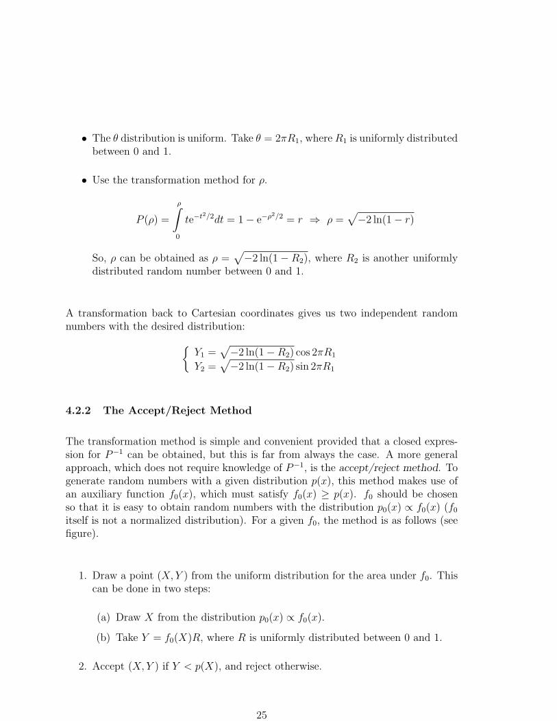
4.2.2 The Accept/Reject Method
The transformation method is simple and convenient provided that a closed expres-sion for P−1 can be obtained, but this is far from always the case. A more generalapproach, which does not require knowledge of P−1, is the accept/reject method. Togenerate random numbers with a given distribution p(x), this method makes use ofan auxiliary function f0(x), which must satisfy f0(x) ≥ p(x). f0 should be chosenso that it is easy to obtain random numbers with the distribution p0(x) ∝ f0(x) (f0
itself is not a normalized distribution). For a given f0, the method is as follows (seefigure).
1. Draw a point (X,Y ) from the uniform distribution for the area under f0. Thiscan be done in two steps:
(a) Draw X from the distribution p0(x) ∝ f0(x).
(b) Take Y = f0(X)R, where R is uniformly distributed between 0 and 1.
2. Accept (X,Y ) if Y < p(X), and reject otherwise.
25

The accepted points (X,Y ) obtained this way will be uniformly distributed in theregion under p. This implies that the X component of the accepted points has thedistribution p(x).
Example: Kahn’s method for normally distributed random numbers.
Consider the distribution
p(x) =
21√2π
e−x2/2 x ≥ 0
0 x < 0
(if a random number with this distribution is given a random sign, a normally dis-tributed random number is obtained).
Use the accept/reject method with
f0 (x) =
√
2
πe−x+1/2 x ≥ 0
0 x < 0
This choice of f0 is OK since
p(x)
f0(x)= e−(x−1)2/2 ≤ 1 ,
and the corresponding probability distribution is
p0(x) =f0(x)
∫ ∞−∞ f0(x)dx
=
e−x x ≥ 00 x < 0
We now follow the steps above:
26

1. Draw (X,Y ) in the area under f0. If R1 and R2 are uniformly distributedbetween 0 and 1, we can put
(a) X = − ln R1 (exponential distribution; see previous example).
(b) Y = f0(X)R2.
2. Accept ifY < p(X) ⇔ R2 < e−(X−1)2/2
This gives us a simple two-step “algorithm”:
1. Put X = − ln R1.
2. Accept X if R2 < e−(X−1)2/2.
How efficient is this method? This depends crucially on the acceptance rate, whichis the area under p (which is 1) divided by the area under f0. In this particularexample, we find an acceptance probability of
1√
2e
π
∞∫
0
e−xdx
≈ 0.76 .
4.2.3 The Veto Algorithm
The ‘radioactive decay’ type of problems is very common. In this kind of problemsthere is one variable t, which may be thought of as giving a kind of time axis alongwhich different events are ordered. The probability that ‘something will happen’ (anucleus decay) at time t is described by a function f(t), which is non-negative in therange of t values to be studied. However, this naıve probability is modified by theadditional requirement that something can only happen at time t if it did not happenat earlier times t′ < t. (The original nucleus cannot decay once again if it alreadydid decay; possibly the decay products may decay in their turn, but that is anotherquestion.)
The probability that nothing has happened by time t is expressed by the functionN (t) and the differential probability that something happens at time t by P(t). Thebasic equation then is
P(t) = −dNdt
= f(t)N (t) .
27

For simplicity, we shall assume that the process starts at time t = 0, with N (0) = 1.
The above equation can be solved easily if one notes that dN /N = d lnN :
N (t) = N (0) exp
−∫ t
0
f(t′) dt′
= exp
−∫ t
0
f(t′) dt′
,
and thus
P(t) = f(t) exp
−∫ t
0
f(t′) dt′
.
With f(t) = c this is nothing but the textbook formula for radioactive decay. Inparticular, at small times the correct decay probability, P(t), agrees well with theinput one, f(t), since the exponential factor is close to unity there. At larger t, theexponential gives a dampening which ensures that the integral of P(t) never canexceed unity, even if the integral of f(t) does. The exponential can be seen as theprobability that nothing happens between the original time 0 and the final time t. Inthe parton-shower language of Quantum Chromo Dynamics, this corresponds to theso-called Sudakov form factor.
If f(t) has a primitive function with a known inverse, it is easy to select t valuescorrectly:
∫ t
0
P(t′) dt′ = N (0) −N (t) = 1 − exp
−∫ t
0
f(t′) dt′
= 1 − R ,
which has the solution
F (0) − F (t) = ln R =⇒ t = F−1(F (0) − ln R) .
If f(t) is not sufficiently nice, one may again try to find a better function g(t), withf(t) ≤ g(t) for all t ≥ 0. However to use the normal accept/reject method withthis g(t) would not work, since the method would not correctly take into accountthe effects of the exponential term in P(t). Instead one may use the so-called vetoalgorithm:
1. start with t0 = 0;
2. select ti = G−1(G(ti−1) − ln R), i.e. according to g(t), but with the constraintthat ti > ti−1,
3. compare a (new) R with the ratio f(ti)/g(ti); if f(ti)/g(ti) ≤ R, then return topoint 2 for a new try;
28

4. otherwise ti is retained as final answer.
It may not be apparent why this works. Consider, however, the various ways in whichone can select a specific time t. The probability that the first try works, t = t1, i.e.that no intermediate t values need be rejected, is given by
P0(t) = exp
−∫ t
0
g(t′) dt′
g(t)f(t)
g(t)= f(t) exp
−∫ t
0
g(t′) dt′
,
where the ratio f(t)/g(t) is the probability that t is accepted. Now consider the casewhere one intermediate time t1 is rejected and t = t2 is only accepted in the secondstep. This gives
P1(t) =
∫ t
0
dt1 exp
−∫ t1
0
g(t′) dt′
g(t1)
[
1 − f(t1)
g(t1)
]
exp
−∫ t
t1
g(t′) dt′
g(t)f(t)
g(t),
where the first exponential times g(t1) gives the probability that t1 is first selected,the square brackets the probability that t1 is subsequently rejected, the followingpiece the probability that t = t2 is selected when starting from t1, and the final factorthat t is retained. The whole is to be integrated over all possible intermediate timest1. The exponentials together give an integral over the range from 0 to t, just as inP0, and the factor for the final step being accepted is also the same, so therefore onefinds that
P1(t) = P0(t)
∫ t
0
dt1 [g(t1) − f(t1)] .
This generalizes. In P2 one has to consider two intermediate times, 0 ≤ t1 ≤ t2 ≤t3 = t, and so
P2(t) = P0(t)
∫ t
0
dt1 [g(t1) − f(t1)]
∫ t
t1
dt2 [g(t2) − f(t2)]
= P0(t)1
2
(∫ t
0
[g(t′) − f(t′)] dt′)2
.
The last equality is most easily seen if one also considers the alternative region 0 ≤t2 ≤ t1 ≤ t, where the roles of t1 and t2 have just been interchanged, and the integraltherefore has the same value as in the region considered. Adding the two regions,however, the integrals over t1 and t2 decouple, and become equal. In general, forPi, the i intermediate times can be ordered in i! different ways. Therefore the totalprobability to accept t, in any step, is
P(t) =∞∑
i=0
Pi(t) = P0(t)∞∑
i=0
1
i!
(∫ t
0
[g(t′) − f(t′)] dt′)i
29

= f(t) exp
−∫ t
0
g(t′) dt′
exp
∫ t
0
[g(t′) − f(t′)] dt′
= f(t) exp
−∫ t
0
f(t′) dt′
, (1)
which is the desired answer.
If the process is to be stopped at some scale tmax, i.e. if one would like to remainwith a fraction N (tmax) of events where nothing happens at all, this is easy to includein the veto algorithm: just iterate upwards in t at usual, but stop the process if noallowed branching is found before tmax.
Usually f(t) is a function also of additional variables ~x. The methods of the precedingsection are easy to generalize if one can find a suitable function g(t, ~x) with f(t, ~x) ≤g(t, ~x). The g(t) used in the veto algorithm is the integral of g(t, ~x) over ~x. Each timea ti has been selected also an ~xi is picked, according to the conditional probabilityg(~x|ti), and the (t, ~x) point is accepted with probability f(ti, ~xi)/g(ti, ~xi).
4.3 Random Number Generators
Random numbers are generally pseudo random numbers on the computer, obtainedby a deterministic algorithm. Whether or not these random numbers are “randomenough” depends on both the algorithm used and the problem at hand. The useof deterministic algorithms may seem strange, but has two major advantages, speedand reproducibility. Reproducibility can be a valuable property when debugging aprogram.
Most programming languages provide some built-in random number generator, butthere are sometimes good reasons not to use these. One possible reason is portability.Another possible reason is that built-in random number generators are not seldomof quite poor quality.
4.3.1 The Linear Congruential Method
A widely used deterministic algorithm for generating random numbers is the linearcongruential method; many random number generators rely on this algorithm orvariants of it.
In its simplest version, this method uses a recursion formula of the form
ij+1 = aij + c mod m
30

to generate a sequence i1, i2, . . . of integers. Putting xj = ij/m, we obtain a nor-malized sequence x1, x2, . . . of numbers between 0 and 1. The hope is that thesenumbers, for a suitable choice of the integer parameters a, c and m (see table inNR), will behave as approximately independent and uniformly distributed randomnumbers.
Clearly, these xj’s are not independent, and therefore it is important to test howstrong the correlations between the xj’s are. One way to do this is as follows.
• x1, x2, . . . should be uniformly distributed on the unit interval from 0 to 1.
• (x1, x2), (x3, x4), . . . should be uniformly distributed on the unit square.
...
• (x1, . . . , xn), (xn+1, . . . , x2n), . . . should be uniformly distributed on the unitcube in n dimensions.
For the linear congruential method with c = 0, it can be shown that all possiblen-tuples (xj+1, . . . , xj+n) fall onto one of at most (n! m)1/n different hyperplanes.This number is not very large; if we, for example, take m = 232 and n = 10, then(n! m)1/n ≈ 42. This shows that this method exhibits correlations that definitely maycause problems in applications where many random numbers are needed.
It is also worth noting that the recursion formula above is periodic, with a period ofm or smaller, so m should be very large.
There are methods that are better than this one; for a discussion, see NR. Neverthe-less, it should be kept in mind that random number generators are not perfect, andthey should be chosen with care in applications where lots of random numbers areneeded.
4.4 Monte Carlo Integration and Summation
Example: Monte Carlo calculation of π.
Consider the first quadrant of the unit circle. Its area (= π/4) can be written as
I =
∫
first quadrant
dxdy
31

Let us see how this integral can be estimated by using random numbers.
Suppose we have N random points drawn from the uniform distribution on the unitsquare. For each point i, we introduce a binary random variable χi such that χi = 1if point i is in the first quadrant of the unit circle, and χi = 0 otherwise. The meanof each χi is I, the area of the first quadrant (since the area of the square is 1). Itfollows that
1
N
N∑
i=1
χi =1
Nno. of points in the first quadrant → I N → ∞
which gives us a method for estimating I (and thereby π).
Let us now generalize this by considering
I =
∫
f(x)p(x)dx
where f(x) is an arbitrary function and p(x) is some probability distribution. Assumethat X1, . . . , XN are independent random variables, all with the distribution p(x).f(X1), . . . , f(XN) are then independent and identically distributed random variables.This means, according to the central limit theorem, that
IN =1
N
N∑
i=1
f(Xi)
is approximately normally distributed for large N , with
• mean 〈IN〉 =
∫
f(x)p(x)dx = I
• variance σ2N = (〈f(X)2〉 − 〈f(X)〉2)/N → 0 as N → ∞
32

Hence, IN may be used as an estimator of I for large N . The method can beimmediately generalized to higher dimensions.
Sums can be dealt with in a similar way. Consider
S =∑
i
f(i)p(i)
where f(i) is an arbitrary function and p(i) is some discrete probability distribution.If I1, . . . , IN are independent random numbers with the distribution p(i), we canestimate S by using
S ≈ SN =1
N
N∑
k=1
f(Ik)
for large N .
4.4.1 Convergence Rate
What about the efficiency of Monte Carlo integration? Let us compare the efficencyof this method in one dimension, D = 1, with that of the Simpson rule.
Consider an integral over an interval of length L, and let Tε denote the amount ofcomputer time needed to achieve an accuracy of O(ε).
• Simpson’s rule
ε ∼ h4 (h step size)Tε ∝ no. of function values ∼ L/h
⇒ Tε ∼ ε−1/4
• Monte Carlo
ε ∼ N−1/2 (N no. of points)Tε ∝ N
⇒ Tε ∼ ε−2
This comparison shows that the convergence of the Monte Carlo method is typicallymuch slower than that of the Simpson rule for D = 1. The strength of the MonteCarlo method is its generality. If, for example, D is large or the boundary of theintegration region is complex, there often are few alternatives to Monte Carlo.
33
4.4.2 Importance Sampling
A Monte Carlo calculation of a given integral
I =
∫
f(x)dx
may use random numbers drawn from any probability distribution p(x) > 0. In fact,with X1, . . . , XN drawn from any given p(x) > 0, we may estimate I as
I =
∫f(x)
p(x)p(x)dx ≈ Ip
N =1
N
N∑
i=1
f(Xi)
p(Xi)
The mean of the estimator IpN is, of course, independent of p, 〈Ip
N〉 = I. The variance〈(Ip
N)2〉 − 〈IpN〉2 depends, by contrast, strongly on p. In order to have a reasonable
performance, it is therefore crucial to make a careful choice of p.
In principle, it is known what the optimal choice of p is, namely p(x) ∝ |f(x)| (seeNR 7.8). In practice, this is of little help because finding the proportionality constantin this relation is as difficult as finding the integral we want to compute. However, itis often possible to make an educated guess of p that is useful, although not perfect.
Example: The Ising model.
The Ising model is a simple model for ferromagnetism. The system consists of Nbinary spin variables σi = ±1 that live on a lattice. In the absence of an externalmagnetic field, the energy E of a configuration σ = (σ1, . . . , σN) is given by
E = −J∑
〈ij〉σiσj
where the sum runs over all nearest-neighbor pairs on the lattice. The thermodynamicbehavior of the system is governed by the Boltzmann weight
p(σ) ∝ e−E(σ)/kT
where k is Boltzmann’s constant and T the temperature. The average of an observableO, the total magnetization say, at temperature T is given by
〈O〉 =∑
σ
O(σ)p(σ) =
∑
σ
O(σ)e−E(σ)/kT
∑
σ
e−E(σ)/kT
34

How can we calculate such an average?
• Exactly, by exhaustive enumeration of all possible states? No, because thenumber of states, 2N , is too large; already for N = 100 (which is a very smallsystem), there are 2100 ∼ (103)10 = 1030 possible states.
• “Naive” Monte Carlo? Here, we would draw configurations σ(1), . . . , σ(J) fromthe uniform distribution p0(σ) = 1/2N = constant, and estimate
〈O〉 ≈(
1
J
J∑
j=1
O(σ(j))e−E(σ(j))/kT
)
×(
1
J
J∑
j=1
e−E(σ(j))/kT
)−1
But E is an extensive quantity, which means that there will be huge fluctuationsin e−E/kT . As a result, the variance is very large and the convergence very slow.
• Importance sampling. If instead we draw σ(1), . . . , σ(J) from the Boltzmanndistribution p(σ), then we can use an estimate
〈O〉 ≈ 1
J
J∑
j=1
O(σ(j))
that does not contain any Boltzmann factor e−E/kT . This is typically an enor-mous improvement. The next question then is how to generate Boltzmanndistributed configurations. A widely used method for this is the Metropolisalgorithm.
4.5 The Metropolis Algorithm
Consider a system with state or configuration space T , and suppose we want tosample some distribution p(σ), σ ∈ T . For simplicity, we assume T to be discrete (asin the Ising model).
The Metropolis algorithm can be thought of as a guided random walk in the statespace T ,
σ1 → σ2 → σ3 → . . .
Here, σn denotes the state of the system at “time” n. The guidance is such that theprobability distribution pn of σn approaches p for large n; that is,
limn→∞
pn(σ) = p(σ) . (2)
35

This is meant to hold irrespective of what the initial distribution p1 is.
A fundamental property of the Metropolis algorithm is that pn+1 is entirely deter-mined by pn; in order to determine pn+1, we do not have to know where the systemwas at time n − 1, n − 2, . . .. A stochastic process with this property is called aMarkov chain. For a Markov chain, the time evolution can be described in terms of atransition matrix W (σ, σ′); W (σ, σ′) being the conditional probability of finding thesystem in state σ at time n + 1, given that it was in state σ′ at time n. Anotherimportant property of the Metropolis algorithm is that the transition matrix W (σ, σ′)does not change with time n.
These two properties imply that the time evolution of pn is given by a simple vector-matrix equation,
pn+1(σ) =∑
σ′
W (σ, σ′)pn(σ′) (3)
with a constant (n independent) matrix W .
The key question now is how to ensure that pn → p as n → ∞, equation (1). Usefulinformation about this can be obtained from the theory for general Markov chainswith constant transition matrices (“stationary” Markov chains). For a general processof this type, it can be shown that equation (1) does hold independent of the initialdistribution if the following two conditions are met:
1. The distribution p is stationary. This means that pn = p ⇒ pn+1 = p. An-other way to say this is that p should be an eigenvector of the matrix W witheigenvalue 1; that is,
p(σ) =∑
σ′
W (σ, σ′)p(σ′) (for all σ)
2. The process is ergodic. Loosely speaking, this means that each state can bereached from each other state. A somewhat more precise formulation of thiscondition can be found in the hand-out for the first computer exercise.
We are not going to prove that these two requirements are sufficient to ensure thatequation (1) holds, but to give an idea of how it works, we will prove two weakerstatements. For this purpose, we need to define the distance between two arbitrarydistributions pa and pb, which can be taken as
‖pa − pb‖ =∑
σ
|pa(σ) − pb(σ)|
36

Statement 1: Suppose p is stationary. Then the distance ‖pn − p‖ is a non-increasingfunction of n.
Proof: Using equation (2) and that p is stationary, we obtain
‖pn+1 − p‖ =∑
σ
| pn+1(σ) − p(σ)|
=∑
σ
∣∣∣
∑
σ′
W (σ, σ′)(pn(σ′) − p(σ′))∣∣∣
6∑
σ
∑
σ′
W (σ, σ′)|pn(σ′) − p(σ′)|
= ‖ pn − p‖( ∑
σ
W (σ, σ′) = 1)
Statement 2: Suppose, in addition to the stationarity of p, that W (σ, σ′) > 0 for allσ, σ′ and that pn 6= p. Then the inequality above is strict,
‖ pn+1 − p‖ < ‖ pn − p‖
Proof: That pn 6= p implies that pn(σ′) − p(σ′) takes on both positive and negativevalues, since pn and p both are normalized distributions. The same must then betrue for W (σ, σ′)(pn(σ′) − p(σ′)), since W (σ, σ′) > 0 for all σ, σ′. From this followsthat the inequality must be strict.
The Metropolis algorithm provides a simple and general way to ensure that condition1 above is met. This is achieved by designing the basic update of the system in sucha way that detailed balance is fulfilled, a condition that is stronger than the condition1 above. How this is done is discussed in the hand-out for the first computer exercise.
Comments
For simplicity, we have here considered discrete systems. The Metropolis algorithmcan be easily applied to continuous systems, too.
The fact that the states generated by the Metropolis algorithm are not independentmakes this method fundamentally different from methods such as the simple trans-formation and accept/reject methods. Methods like these two are sometimes calledstatic, and methods like the Metropolis algorithm are then called dynamic.
37

5 Optimization (minimization/maximization)
[NR: 9.6, 10.0, 10.1, 10.4, 10.5, 10.6, 10.9]
Optimization is a wide field. Sometimes there exists a well-established method thatcan be used in a black-box manner, but many optimization problems are true chal-lenges.
Suppose we want to minimize some function f(x) in D dimensions, x ∈ RD. How toproceed depends on a number of things, such as
• What is the dimensionality D?
• Are there constraints on x?
• Is the problem linear or non-linear?
• Is f such that minimization is a smooth downhill process, or are there traps inthe form of local minima?
• Do we want the global minimum of f , or is it sufficient to make a local mini-mization?
• Do we have access to derivatives of f?
In this section, we first look at a simple and general scheme called simulated annealingthat can be tried if the aim is to make a global optimization (section 5.1). We thendiscuss a few different methods for local optimization; first, the downhill simplexmethod without derivatives (section 5.2), and then the conjugate-gradient and quasi-Newton methods that do use derivatives (sections 5.3.2 and 5.3.3). We end with afew words on optimization in the presence of constraints (section 5.4).
But first of all, a general remark on precision. Suppose we want to minimize a functionf(x) (assume, for simplicity, D = 1). A Taylor expansion about the minimum xmin
givesf(x) ≈ f(xmin) + 1
2(x − xmin)
2 f ′′(xmin) (x near xmin)
since f ′(xmin) = 0. Near xmin, the roundoff error in f(x) is & ε|f(xmin)|, where ε isthe relative floating-point precision. If now |x−xmin| is so small that |f(x)−f(xmin)|is comparable to the roundoff error, then we cannot expect to be able to come closerto xmin, irrespective of what search method we use. This gives an estimate of thesmallest possible error, ∆x, in xmin:
38
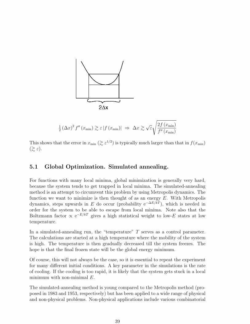
12(∆x)2 f ′′ (xmin) & ε |f (xmin)| ⇒ ∆x &
√ε
√
2f (xmin)
f ′′ (xmin)
This shows that the error in xmin (& ε1/2) is typically much larger than that in f(xmin)(& ε).
5.1 Global Optimization. Simulated annealing.
For functions with many local minima, global minimization is generally very hard,because the system tends to get trapped in local minima. The simulated-annealingmethod is an attempt to circumvent this problem by using Metropolis dynamics. Thefunction we want to minimize is then thought of as an energy E. With Metropolisdynamics, steps upwards in E do occur (probability e−∆E/kT ), which is needed inorder for the system to be able to escape from local minima. Note also that theBoltzmann factor ∝ e−E/kT gives a high statistical weight to low-E states at lowtemperature.
In a simulated-annealing run, the “temperature” T serves as a control parameter.The calculations are started at a high temperature where the mobility of the systemis high. The temperature is then gradually decreased till the system freezes. Thehope is that the final frozen state will be the global energy minimum.
Of course, this will not always be the case, so it is essential to repeat the experimentfor many different initial conditions. A key parameter in the simulations is the rateof cooling. If the cooling is too rapid, it is likely that the system gets stuck in a localminimum with non-minimal E.
The simulated-annealing method is young compared to the Metropolis method (pro-posed in 1983 and 1953, respectively) but has been applied to a wide range of physicaland non-physical problems. Non-physical applications include various combinatorial
39

optimization problems, such as the traveling salesman problem. In this problem,there are N cities to be visited, and each city is to be visited precisely once. The taskis to minimize the distance that the salesman has to travel. Solving this problem ex-actly is possible only for small N , because the number of alternative routes, (N −1)!,grows rapidly with N . With simulated annealing it becomes possible to study largerN . A simulated-annealing program for this problem can be found in NR 10.9.
5.2 Local Optimization without Derivatives.The Downhill Simplex Method
When searching for the minimum of a function f(x) in D dimensions, it is of help toknow the gradient ∇f(x), because −∇f(x) is the direction in which the decrease off(x) is fastest (locally). In what direction should one search if the gradient ∇f(x)is not available?
A simple and general scheme that does not rely on information on the gradient is thedownhill simplex method. A simplex is a geometrical object with one more vertexthan dimension: a line segment for D = 1, a triangle for D = 2, a tetrahedron forD = 3, and so on. In the downhill simplex method, the simplex is a dynamic objectthat can grow and shrink. When it reaches a minimum, it gives up and shrinks downaround it.
The method proceeds iteratively, starting from some simplex with vertices x1, . . . ,xD+1
which we assume ordered so that f(xD+1) ≤ f(xD) ≤ . . . ≤ f(x1). The elementarymove can be seen as an attempt to improve the worst point, x1, and is as follows.
Calculate the center of the face defined by the points x2, . . . ,xD+1,
xmean ≡ 1
D
D+1∑
i=2
xi
Since all these D points are better than x1, it makes sense to try to move x1 in thedirection of xmean. Therefore, the next step is to reflect x1 across this face to
xa = xmean + (xmean − x1)
40

Whether this point is accepted or not depends on the value of f(xa):
• If f(xD+1) < f(xa) < f(x2), replace x1 by xa.
• If f(xa) < f(xD+1), try a larger step (the direction seems good) to
xb = xmean + 2(xmean − x1)
x1 is then replaced by the best of xa and xb.
• If f(xa) > f(x2), try instead a smaller step to
xc = xmean + 12(xmean − x1)
If f(xc) < f(x2), replace x1 by xc. Otherwise, try an even smaller step to
xd = xmean − 12(xmean − x1)
If f(xd) < f(x2), replace x1 by xd. If this attempt also fails, the simplex is toolarge to give a good idea of what direction to choose. Therefore, we now giveup and shrink all the vertices towards the best one
xi → xi + 12(xD+1 − xi) i = 1, . . . , D
This update is iterated untill the values are no longer improving, according to somestopping criterion.
41

5.3 Local Optimization with Derivatives
5.3.1 Successive Line Minimizations
Many methods for multidimensional minimization are based on successive line mini-mizations. Usually, the gradient of the function is used to decide on what lines to beconsidered. The actual minimization along each of these lines may or may not usederivatives.
For one-dimensional minimization, there exist methods that are relatively robust andfast. Assume that we have such a method at our disposal and want to minimize afunction f(x), x ∈ RD. We may then proceed as follows.
1. Pick a starting point x0 and a direction h0.
2. Determine λ0 by minimization of f along the line λ 7→ x0 + λh0.
3. Put x1 = x0 + λ0h0 and select a new direction h1.
4. Determine λ1 by minimization of f along the line λ 7→ x1 + λh1.
5. . . .
But what directions hi should we use?
• The D basis vectors ei?No, we don’t want to be restricted to these directions (see figure in NR 10.5).
• hi = −∇f(xi)?This is called steepest descent and may seem like a natural choice. However,this method has an unwanted property that tends to make it inefficient (seefigure in NR 10.6): consecutive directions hi and hi+1 are, by construction,orthogonal. To see this, note that xi+1 is obtained by minimizing f along theline λ 7→ xi + λhi, which implies that
0 =df(xi + λhi)
dλ
∣∣∣λ=λi
= ∇f(xi+1) ·d(xi + λhi)
dλ= (−hi+1) · hi
Conjugate directions
42

Near minima, quadratic approximations are generally good. Let us therefore considera quadratic function
f(x) = 12x · Ax − b · x + c
x and b ∈ RD
A symmetric, positive definite D × D matrixc number
(A is assumed positive definite so that f has a minimum). If we were to minimizethis f by successive line minimizations, how should we then choose the directions hi?
When minimizing f , we are searching for an x at which all the components of thevector ∇f(x) = Ax − b vanish. By construction, one component of ∇f(xi+1) hasto be zero, ∇f(xi+1) · hi = 0. Can we by a suitable choice of the hi’s see to that∇f(xi+1) · hi−1 = 0, too?
hi−1 · ∇f(xi+1) = hi−1 · [A(xi + λihi) − b] =
= hi−1 · [∇f(xi) + λiAhi]
= λihi−1 · Ahi
So,hi−1 · ∇f(xi+1) = 0 if hi−1 · Ahi = 0
hi−1 and hi are called conjugate, or A orthogonal, if this condition is fulfilled.
5.3.2 The Conjugate Gradient Method
This is a method based on successive line minimizations in which the directions hi
are conjugate if the function is quadratic. This makes the method efficient for suchfunctions. For a general function, the method is expected to work well if we aresufficiently close to the minimum.
The algorithm is simple to formulate. For convenience, put gi = −∇f(xi), where f isthe function to be minimized. Let x0 be an arbitrary starting point and take h0 = g0.Pairs (x1, h1), (x2, h2),. . . are then generated by using the recursion formulas:
xi+1 = xi + λihi where λi is determined by line minimization
hi+1 = gi+1 + γihi where γi =gi+1 · gi+1
gi · gi
(with γi = 0 this would be the steepest descent method).
The choice of the parameter γi is such that if
f(x) = 12x · Ax − b · x + c
43

(as above), then hi · Ahi+1 = 0 and also hi+1 · Ahi = 0, since A is symmetric.
In fact we will show something more general, namely that for such f , the followingorthogonality relationships hold
hi · Ahj = 0 (i 6= j)gi · gj = 0 (i 6= j)gi · hj = 0 (i > j)
and that we can write
λi =gi · hi
hi · Ahi
=gi · gi
hi · Ahi
(i = 0, 1, . . .)
We will prove this using induction, i.e. assuming it holds for all i, j ≤ n, we will showthat it holds also for i, j ≤ n + 1.
First we look at some general relationships, noting that hi ·gi+1 = 0 by construction.
So, we have
0 = hi·gi+1 = hi·(b−Axi+1) = hi·(b−Axi−λiAhi) = hi·(gi−λiAhi) = hi·gi−λihi·Ahi
and
λi =gi · hi
hi · Ahi
.
Also,gi · hi = gi · gi + γi−1gi · hi−1 = gi · gi
so we can write
0 = hi+1 · Ahi = (gi+1 + γihi) ·gi − gi+1
λi
where we know that gi+1 · gi = 0, hi · gi+1 = 0 and hi · gi = gi · gi, so
0 =1
λi
(γigi · gi − gi+1 · gi+1) ⇒ γi =gi+1 · gi+1
gi · gi
Now, assuming that gi · gj = hi ·Ahj = 0 for all i 6= j with i, j ≤ n (this is certainlytrue for n = 1) we need to show that it is true for all i 6= j with i, j ≤ n + 1:
gn+1 · gi = gn · gi − λnhn · Agi = −λnhn · Agi.
For i = 0 and i = n this is zero, otherwise we have
= −λnhn · A(hi − γi−1hi−1) = 0.
44

Similarly we have for hn+1 · Ahi, which is zero for i = n, otherwise
hn+1 · Ahi = gn+1 · Ahi + γnhn · Ahi = gn+1 ·gi − gi+1
λi
= 0.
We also need to show that everything holds for n = 1:
Clearly g1 · h0 = g1 · g0 = 0. Also
h0 · Ah1 = h1 · Ah0 = (g1 + γ0g0) ·g0 − g1
λ0
=1
λ0
(γ0g0 · g0 − g1 · g1) = 0 .
In particular, this shows that the vectors gi are pairwise orthogonal. This can holdfor at most D different gi 6= 0 in D dimensions. Hence, gi = 0 for some i ≤ D. But ifgi = 0, then xi is the solution we want. This means that the method needs at most Dsteps to find the minimum. This holds when the function is quadratic. For a generalf the orthogonality relations are at best approximate, and there is no guarantee ofconvergence within a finite number of steps. In this case, the recursion formulas areiterated untill some stopping criterion is fulfilled. Note that the algorithm is writtenin such a way that it can be directly applied to general functions f .
Solution of linear equations by the conjugate gradient method
Suppose we want to solve a linear equation system
Ax = b
where A is a symmetric, positive definite matrix. One approach to this problem isto make use of the fact that the solution must be the minimum xmin of the function
f(x) = 12x · Ax − b · x ,
because xmin satisfies∇f(xmin) = Axmin − b = 0
So, in principle, we can solve our linear algebra problem by using a minimizationmethod such as the conjugate-gradient method. Is this a good approach? It can becomputationally convenient if the matrix A is large but sparse (that is, A has manyelements but relatively few of them are nonzero). The reason that the conjugategradient method is interesting in this case is that the matrix A enters the algorithmonly through expressions of the type A × (vector), which makes it relatively easy totake advantage of the sparseness of the matrix.
45

5.3.3 The Quasi-Newton Method
Minimizing f(x) can be viewed as solving ∇f(x) = 0, which is a system of D generallynon-linear equations,
∂1f(x) = 0...∂Df(x) = 0
Suppose we are at some point x. A Taylor expansion about this point gives
f(x′) = f(x) + (x′ − x) · ∇f(x) + 12(x′ − x) · A(x)(x′ − x) + . . .
where A(x) is the so-called Hessian matrix with elements Aij(x) = ∂i∂jf(x). Bytaking the gradient with respect to the primed variables of both sides of this equation,we obtain
∇f (x′) = 0 + ∇f(x) + A(x)(x′ − x) + . . .
From this we see that if the omitted higher-order terms can be neglected, and if x′
is given by
x′ − x = −A−1(x) · ∇f(x) ,
then we have ∇f(x′) = 0. The Newton method would be to iterate this equation tillsome stopping criterion is fulfilled.2
This method has, however, two disadvantages: first, the second derivatives ∂i∂jfare needed; and second, the equation system A(x)y = ∇f(x) must be solved fory = A−1(x) · ∇f(x) at each step. Usually, this makes the method impractical, butthere are exceptions, like the Levenberg-Marquardt method for χ2 minimization.
The so-called quasi-Newton method circumvents these two problems. This methodis based on successive line minimizations and can be written as
xi+1 = xi − λiHi · ∇f(xi) ,
where the parameter λi is determined by line minimization, and Hi is a D×D matrixconstructed so that Hi → A−1 as i → ∞. For details, see NR 10.7.
The quasi-Newton method is often comparable in efficiency to the conjugate-gradientmethod, but requires more memory if D is large; the memory requirement scales asD2 for the quasi-Newton method and as D for the conjugate-gradient method.
2The “standard” Newton method for a one-dimensional problem g(x) = 0 is given by the recur-sion formula x′ − x = −g(x)/g′(x).
46

5.4 Constrained minimization
5.4.1 Linear optimization/linear programming
Constrained minimization with a linear cost function and linear constraints is referredto as linear optimization or linear programming. For such problems there is a well-established method called the Simplex method, which is described in NR 10.8.
For a simple example of such a problem, consider the cost function f(x1, x2) = x1+x2
with the constraints
2x1 + x2 ≤ 2 x1 + 2x2 ≤ 2 x1, x2 ≥ 0
Since the gradient ∇f = (1, 1) is constant, the desired minimum must be somewhereon the boundary, and it is easy to see that the solution is (x1, x2) = (0, 0).
5.4.2 Lagrange multiplier
Suppose we want to minimize a function f(x) subject to the constraint u(x) = 0,x ∈ RD. One possible approach is to look for stationary points of the auxiliaryfunction f(x, λ) = f(x)+λu(x), where λ is called a Lagrange multiplier. A stationarypoint of this function is a solution of the D + 1 equations
0 = ∇xf(x, λ) = ∇f(x) + λ∇u(x)
0 =∂f
∂λ= u(x)
The last equation is just the constraint, which says that x must fall onto the hy-persurface defined by u(x) = 0. The gradient ∇u(x) is normal to this surface. Thefirst D equations imply that ∇f(x) is parallel (or anti-parallel) to ∇u(x). If t is an
47

arbitrary unit vector in the tangential plane of the surface u(x) = 0, it follows that
∂f
∂t= t · ∇f = 0 .
This means that the derivative of f is zero in every “allowed” direction, which isprecisely what we want.
This method is widely used in analytical calculations. As a numerical method, ithas the disadvantage that a system of generally non-linear equations must be solved,which can be tricky.
5.4.3 Soft constraints
Consider the same task once more; minimize f(x) subject to the constraint u(x) = 0.A method that often works better numerically than the previous one is to introducethe constraint in a soft manner, by forming the auxiliary function
f(x, Λ) = f(x) + Λu(x)2
This function is to be minimized. Numerically, this is generally more convenient thansolving a system of equations. The desired solution is obtained by extrapolatingresults for large Λ, xΛ, to Λ = ∞, x = limΛ→∞ xΛ. Note that the penalty termΛu(x)2 grows large as Λ → ∞ unless x satisfies u(x) = 0.
6 Ordinary Differential Equations (ODE)
[NR: 16.0, 16.1, 16.3, 16.6 (16.2, 16.4, 16.7)]
48

6.1 Introduction
This section deals with numerical integration of ODEs. We will discuss methods forsolving systems of first-order ODEs
dy1
dx= f1 (x, y1, . . . , yn)
...dyn
dx= fn (x, y1, . . . , yn)
for given initial values of all the components yi at some “time” x0 (for a discussionof boundary value problems, see chapter 17 of NR). In vector notation, this initialvalue problem can be written as
dy
dx= f(x,y) y(x0) = y0 .
Looking only at first-order ODEs is not a strong limitation, because any nth orderODE of the form
dny
dxn= f
(
x, y,dy
dx, . . . ,
dn−1y
dxn−1
)
can be written as a system of first-order ODEs by the transformation
y1 = y
y2 =dy
dx...
yn =dn−1y
dxn−1
⇒
dy1
dx= y2
dy2
dx= y3
...dyn
dx= f (x, y1, . . . , yn)
For convenience, we will often assume that n = 1. This does not mean that thesemethods work only for n = 1; on the contrary, generalizing to n > 1 is typically easy.
Example: Consider the one-dimensional Newton equation
md2x
dt2= −V ′(x)
Putting x1 = x and x2 = dx/dt, we obtain the first-order ODEs
dx1/dt = x2
dx2/dt = −V ′(x1)/m
49

which are the corresponding Hamilton equations.
(Hamilton’s equations of motion are given by dx/dt = ∂H/∂p and dp/dt = −∂H/∂x,where p = m dx/dt and H = p2/2m + V (x).)
6.2 Euler’s Method
Consider the first-order ODEdy
dx= f(x, y) .
To solve this equation numerically, we discretize x using a step size h:
xn = x0 + nh n = 0, 1, . . .yn = y (xn)
Approximating the derivative with a simple forward difference,
dy
dx
∣∣∣x=xn
=yn+1 − yn
h+ O (h) ,
we obtain the recursion formula
yn+1 = yn + hf(xn, yn) .
This can be used to calculate yn for arbitrary n, starting from a given y0.
This is called the Euler method. Its local truncation error is ∼ h2 (one step), whichmakes the global truncation error ∼ h (this is how the error scales for a fixed totallength in x).
A method whose global error scales as hn is called an nth-order method, so the Eulermethod is a first-order method.
Low-order methods require small step sizes h, which makes the required number ofsteps large. Therefore, the computational cost tends to be high.
6.3 Taylor Expansion
A straightforward way to reduce the truncation error is to make use of the Taylorexpansion
y (xn + h) = yn + hdy
dx
∣∣∣∣x=xn
+h2
2
d2y
dx2
∣∣∣∣x=xn
+ . . .
50

where dy/dx = f and
d2y
dx2=
df
dx= ∂xf + ∂yf · dy
dx= ∂xf + ∂yf · f .
Keeping the first three terms we obtain
y (xn + h) = yn + hf (xn, yn) +h2
2[∂xf (xn, yn) + f (xn, yn) ∂yf (xn, yn)] + O
(h3
)
which is a second-order method, or one order better than the Euler method. Clearly,the same procedure can be used to obtain higher-order methods. This approach has,however, the disadvantage that higher and higher derivatives of the function f willbe needed.
6.4 The Runge-Kutta Method
The Runge-Kutta method avoids this problem — no derivatives of f are needed.Instead, the estimator yn+1 is constructed using values of f itself at carefully chosenpoints between xn and xn+1. By increasing the number of points, the order of themethod can be increased.
6.4.1 Second-Order Runge-Kutta (local error ∼ h3)
Consider the ansatz
k1 = hf (xn, yn)
k2 = hf (xn + mh, yn + mk1)
yn+1 = yn + ak1 + bk2
which combines two different f values and has three parameters: a, b and m.
The idea is to determine these three parameters so that the error becomes as smallas possible. For this purpose, we make a Taylor expansion of yn+1 about x = xn:
51

k2 = hf(xn, yn) + mh2∂xf (xn, yn) + mh2f (xn, yn) ∂yf (xn, yn) + O(h3
)⇒
yn+1 = yn + (a + b) hf (xn, yn) + bmh2 (∂xf (xn, yn) + f (xn, yn) ∂yf (xn, yn)) + O(h3)
By comparing this expression with the Taylor expansion of the exact solution y(xn+h)(see above), we see that the local error becomes O(h3) if
a + b = 1 and bm = 1/2
This is the best that can be achieved with this ansatz — to eliminate the O(h3) errorterm we would need more points.
The two equations for a, b and m have a one-parameter family of solutions. We can,for example, take
a = 0, b = 1, m = 12
as in NR, or
a = b = 12, m = 1
which is called Heun’s method.
6.4.2 Fourth-Order Runge-Kutta
Higher-order Runge-Kutta methods can be obtained by adding more points. Thisgives improved accuracy at the cost of increased complexity. A very popular com-promise is the fourth-order scheme given by Eq. 16.1.3 in NR, which requires fourf evaluations. One reason that this scheme is so popular is that in order to get afifth-order scheme, it turns out that six (and not five) points are needed.
52

k1 = hf(xn, yn)
k2 = hf(xn + h/2, yn + k1/2)
k3 = hf(xn + h/2, yn + k2/2)
k4 = hf(xn + h, yn + k3)
yn+1 = yn + k1/6 + k2/3 + k3/3 + k4/6 + O(h5)
6.5 Adaptive Step Size
So far, we have assumed that the step size h is held constant throughout the integra-tion. However, the function f(x, y) may be very different in different parts of space.As a result, there may exist both “easy” regions where a large step can be used and“difficult” ones where a much smaller step size is required.
Therefore, it is often very useful to vary the step size. A natural choice is to vary thestep size in such a way that the local error is kept at a constant level. For that, weneed to have an estimate of the local error.
A convenient way to estimate the local error is by step doubling. This means thatwe repeat all calculations using a step size twice as large. By comparing the twocalculations, we get an estimate of the local error.
To see how this works, consider fourth-order Runge-Kutta, for which the local errorscales as h5. Let y(x + h; h/2) and y(x + h; h) denote the estimates of the exactsolution y(x + h) that are obtained by using two steps of size h/2 and one step ofsize h, respectively. For small h, these estimates should behave as
y(x + h; h/2) − y(x + h) ∼(
h
2
)5
c(x) + O(h6)
y(x + h; h) − y(x + h) ∼ h5c(x) + O(h6)
where c(x) is some unknown function. The quantity ∆ = |y(x+h; h)−y(x+h; h/2)|provides a rough estimate of the error in y(x + h; h). To keep the local error undercontrol, we may require that ∆ < ∆tol, where ∆tol is a predetermined tolerance level.
If ∆ > ∆tol, we redo the calculation using a smaller step size h′. How small the newstep size h′ should be can be estimated by using that ∆ ∼ h5. This gives
h′ ≈ S
(∆tol
∆
)1/5
h
53

where h is the step size that gave us ∆. S is a “safety” factor that is supposed to beless than 1.
If, on the other hand, ∆ ≪ ∆tol, the step size should be increased. How much it canbe increased can also be estimated by using that ∆ ∼ h5.
The gain from using an adaptive step size can be huge compared to the cost of theadditional calculations that are needed to keep track of the local error.
6.6 The Modified Midpoint Method
Consider the same first-order ODE as before,
dy
dx= f(x, y) .
A central-difference approximation of the derivative,
dy
dx
∣∣∣x=xn
=yn+1 − yn−1
2h+ O
(h2
),
gives us the so-called midpoint method,
yn+1 = yn−1 + 2hf(xn, yn) ,
with a local error of O(h3). This is a “two-point” method, in which both yn and yn−1
are needed in order to obtain yn+1.
(Compare this with the second order Runge-Kutta method with a = 0: yn+1 =yn + hf(xn + h/2, yn + hf(xn, yn)/2) ”=” yn + hf(xn+1/2, yn+1/2))
The modified midpoint method has three components:
1. An initial Euler step to get a second starting value:
y1 = y0 + hf(x0, y0)
2. N − 1 steps with the midpoint method:
yn+1 = yn−1 + 2hf(xn, yn) n = 1, . . . , N − 1
3. A “correction” of the last value yN :
y(x0 + H; h) = 12(yN + yN−1 + hf (xN , yN))
where H = Nh. y(x0 + H; h) is the final estimate, for step size h, of the exactsolution y(x0 + H).
54

For fixed x0 and H and even N , it has been shown (by Gragg) that
y (x0 + H; h) − y (x0 + H) = c1h2 + c2h
4 + ...
In other words, the truncation error contains only even powers of h, a situation wehave encountered before (see Romberg’s integration method). This property makesthe method well suited for Richardson extrapolation.
The so-called Bulirch-Stoer method is based on the modified midpoint method and aRichardson-like extrapolation (but with rational functions rather than polynomials).This method can be a good choice if high accuracy is needed.
6.7 Predictor-Corrector Methods
All methods discussed so far have been explicit in that yn+1 could be calculated ina direct manner, given one or more input values. There are also implicit methods,in which an equation must be solved in order to obtain yn+1. Implicit methods havetheir advantages, as will be seen below in the discussion of stability. A simple exampleof an implicit method is obtained by applying the trapezoidal rule for integration tothe equation dy/dx = f(x, y). This gives
yn+1 − yn =
xn+1∫
xn
f (x, y) dx ≈ h
2[f(xn, yn) + f(xn+1, yn+1)] (i)
This equation for yn+1 can be solved by using Newton’s method for root finding.Another possibility is to use functional iteration. Consider the recursion formula
y(k+1) = g(y(k)) g(y) ≡ yn +h
2[f(xn, yn) + f(xn+1, y)] (ii)
The solution yn+1 to equation (i) is a fixed point of this formula; that is, yn+1 =g(yn+1). If y(k) is close to yn+1, we may linearize the recursion formula:
y(k+1) = g(yn+1 + y(k) − yn+1
)
≈ g (yn+1) +(y(k) − yn+1
) h
2∂yf (xn+1, yn+1)
⇒ y(k+1) − yn+1 ≈(y(k) − yn+1
) h
2∂yf (xn+1, yn+1)
This shows that if our initial guess y(0) is close enough to yn+1 for the linearizationto be OK, and if h is small enough that |h∂yf(xn+1, yn+1)/2| < 1, then |y(k) − yn+1|decreases with k. The desired value yn+1 can then be found by iteration.
55

Predictor-corrector methods use some recursion formula like (ii) to improve on aninitial guess of yn+1. The recursion formula is applied a fixed number of times,and not until some convergence criterion is fulfilled, which makes predictor-correctormethods explicit rather than implicit.
A simple example of a predictor-corrector method, based on the trapezoidal rule, is:
y(0) = yn + hf(xn, yn) “predictor” step
yn+1 = y(1) = yn +h
2[f(xn, yn) + f(xn+1, y
(0))] “corrector” step
Note that this is equivalent to the second order Runge–Kutta with a = b = 1/2 andm = 1.
A widely used, more advanced predictor-corrector method is the Adams-Bashforth-Moulton method (see NR 16.7).
6.8 Stability
If n > 1, it may happen that different components yi evolve at very different speeds.The problem is then called stiff. Stiff problems are generally hard to solve.
Example: Considerdy
dx= −Ay y(0) = y0
where y is a vector with two components and A is a 2 × 2 matrix. Assume that
Avi = λivi (i = 1, 2) λ2 ≫ λ1 > 0
and that y0 = c1v1 + c2v2 for some c1, c2. The exact solution is then given by
y(x) = c1e−λ1xv1 + c2e
−λ2xv2
as can be easily verified. Here, the second term decays much faster than the firstone, because λ2 ≫ λ1. As a result, the second term is not very relevant if we areinterested in “timescales” x & 1/λ1.
Suppose we want to solve this problem numerically by using the Euler method. Thisgives us the recursion formula
yn+1 = yn + h(−Ayn) = (1 − hA)yn
56

(where 1 denotes the unit matrix) which can be easily solved:
yn = (1 − hA)ny0 =
= c1(1 − hA)nv1 + c2(1 − hA)nv2
= c1(1 − hλ1)nv1 + c2(1 − hλ2)
nv2
If we take the limit h → 0 for fixed x = nh, we should recover the exact solution,and this is indeed the case, because
(1 − hλi)n = (1 − λix/n)n → e−λix n → ∞ (h → 0) .
Stability requires that |1−hλi| ≤ 1 for i = 1, 2 (otherwise two solutions correspondingto slightly different initial values will diverge exponentially), and for this to hold itis necessary to take h very small if λ2 is large,
1 − hλ2 ≥ −1 ⇒ h ≤ 2/λ2 .
Suppose now we want to study the behavior at large “timescales”, x & 1/λ1. Thenumber of steps needed will then be very large, x/h & λ2/2λ1. Note that it is therapidly decaying, “uninteresting” component that dictates what step size we can use.
The Implicit Euler Method
If instead of a forward difference we use a backward difference to approximate thederivative,
dy
dx
∣∣∣x=xn
≈ yn − yn−1
h,
we obtain the so-called implicit Euler method. This may look like a minor modifi-cation, but the stability properties change drastically. The recursion formula for theimplicit Euler method is
yn = yn−1 + h(−Ayn) ⇒ yn = (1 + hA)−1yn−1
which has the solution
yn = c1(1 + hλ1)−nv1 + c2(1 + hλ2)
−nv2 .
Again, it is easy to verify that the exact solution is recovered as h → 0 for fixedx = nh. The relative error in the second term will be large unless h is very small, butthis time this error is small in absolute numbers — |1/(1 +λih)| ≤ 1 for all h > 0, sothe stability problems have disappeared. This is a major advantage compared to theprevious method. The disadvantage is that we have to solve an implicit equation foryn for each n, which can be prohibitively time-consuming.
57

Example: Stiff problems are common in physics, especially for systems with manydegrees of freedom. As a not obvious example of a stiff problem, consider an idealring polymer with potential energy
V = 12
N∑
i=1
(xn − xn+1)2 (xN+1 = x1)
and monomer units of mass 1.
The equations of motion for this system are (n = 1, . . . , N)
d2xn
dt2= −∇xn
V =
= −12∇xn
[(xn − xn−1)
2 + (xn − xn+1)2 + xn independent terms
]
= xn−1 + xn+1 − 2xn
The general solution can be written as
xn(t) = A + Bt +N−1∑
k=1
[Ck cos
(2πkn
N− ω(k)t
)+ Dk sin
(2πkn
N− ω(k)t
)]
where A, B, Ck and Dk are constant vectors (determined by the initial conditions)and ω(k) = 2 sin πk/N . The fastest mode corresponds to k = N/2 (if N even) andhas a frequency of ωmax = 2. The k = 1 and k = N − 1 modes are the slowest ones,with a frequency of ωmin = 2 sin π/N .
Now, if a method like the explicit Euler method is applied to this system, then thestep size must satisfy 1 & hωmax for the integration to be stable. This means thata large number of steps will be needed in order to see a significant change in modeswith ω = ωmin, which are those with longest wavelength; the number of steps requiredto integrate up to t = 1/ωmin is
1/ωmin
h&
ωmax
ωmin
=1
sin(π/N)∼ N
π→ ∞ N → ∞
58
So, the number of steps needed to explore the long-wavelength or large-scale prop-erties of the system increases with N . The computer time required for each stepincreases, of course, too.
6.9 Molecular Dynamics (MD)
Classical MD (where quantum-mechanical and relativistic effects are ignored) amountsto integrating Newton’s or Hamilton’s equations of motion for a system of particles,
H =N∑
i=1
p 2i
2mi
+ V (x1, . . . ,xN)
dxi
dt= pi/mi
dpi
dt= −∇xi
V (i = 1, . . . , N)
MD simulations can be used to study both transport and equilibrium properties, andare widely used not least in chemistry. The potential V may contain, for example,Coulomb interactions and van der Waals terms.
Integrating the equations of motion above leaves, of course, the energy E = Hinvariant (dH/dt = 0), as can be easily verified. Nevertheless, molecular dynamicscan be used for calculating equilibrium averages in the canonical ensemble, where theenergy is fluctuating. Such an average can be written as
〈O〉 =
∫
Oρcand3Nxd3Np
ρcan =e−E/kT
∫
e−E/kTd3Nxd3Np
To be able to do this, it is clear that some mechanism must be added to enablethe system to make jumps in energy. One solution is to use a so-called Andersenthermostat, which gives us the two-component algorithm:
1) Ordinary MD; that is, integration of the equation of motions.
2) “Stochastic collisions”. At randomly chosen or predetermined times t, the mo-menta of the particles are refreshed, by drawing new values from the equilibriumdistribution:
pi → p′i where P (p′
i) ∝ exp(−(p′
i)2/2mikT
)
59

Having added these collisions, canonical ensemble averages can be obtained as timeaverages:
∫
Oρcand3Nxd3Np = lim
T→∞
1
T
T∫
0
O (x (t) , p (t)) dt
Assuming that the process is ergodic, this can be justified by showing that ρcan isstationary. That ρcan is stationary under the stochastic collisions is obvious, sincethe new p′
i is drawn from this distribution. That ρcan is stationary under integrationof the equations of motion follows from Liouville’s theorem. This theorem says thatthe flow in phase space (6N -dimensional) under the equations of motion is such thatthe time evolution of a distribution ρ(x, p, t) must satisfy
dρ
dt=
∂ρ
∂t+
N∑
i=1
(
∇xiρ · dxi
dt+ ∇pi
ρ · dpi
dt
)
= 0 .
So, ρ doesn’t change along the trajectories in phase space (the flow is incompress-ible). If ρ = ρ(H(x, p), t), it can be easily shown that the sum in the expression fordρ/dt vanishes, which implies that ∂ρ/∂t = 0. In particular, this shows that ρcan isstationary, ∂ρcan/∂t = 0.
6.10 Numerical Integration of the Equations of Motion
Suppose we integrate the equations of motion above from time 0 to some time t. Thisdefines a mapping T (t) of phase space onto itself:
T (t) : R6N ∋ (x(0), p(0)) 7→ (x(t), p(t)) ∈ R6N
Two important properties of this mapping are:
60
• By Liouville’s theorem, it conserves phase space volume — the Jacobian
∣∣∣∣
∂(x(t), p(t))
∂(x(0), p(0))
∣∣∣∣= 1
• It is time reversible in the sense that
(xA, pA) 7→ (xB, pB) ⇒ (xB,−pB) 7→ (xA,−pA)
When using a discretized version of the equation of motions, these properties aregenerally lost — they hold approximately only. There are, however, discretizationmethods such that these two properties remain exact.
6.10.1 The Leapfrog Method
This method is not very accurate (the local error is O(h3)), but has the advantagethat it is time reversible and preserves phase space volume. It combines two differentelementary steps that represent Euler steps in x and p, respectively:
Ex(h) :
xi(t) 7→ xi(t + h) = xi(t) + hpi/mi
pi(t) 7→ pi(t + h) = pi(t)
Ep(h) :
xi(t) 7→ xi(t + h) = xi(t)pi(t) 7→ pi(t + h) = pi(t) − h∇xi
V (t)
for i = 1, ..., N .
Let S denote the mapping
xi → xi
pi → −pi(i = 1, . . . , N)
An arbitrary mapping M is then time reversible (see above) if M−1 = SMS. It canbe easily verified that Ex(h) and Ep(h) both have this property, but
[Ex (h) Ep (h)]−1 = Ep (h)−1 Ex (h)−1
= SEp (h) Ex (h) S 6= SEx (h) Ep (h) S
The leapfrog method L(h) is obtained by taking a symmetric product,
L(h) = Ex(h/2)Ep(h)Ex(h/2)
61
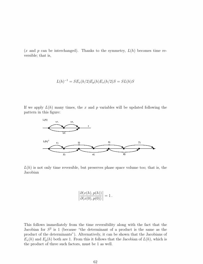
(x and p can be interchanged). Thanks to the symmetry, L(h) becomes time re-versible; that is,
L(h)−1 = SEx(h/2)Ep(h)Ex(h/2)S = SL(h)S
If we apply L(h) many times, the x and p variables will be updated following thepattern in this figure:
L(h) is not only time reversible, but preserves phase space volume too; that is, theJacobian
∣∣∣∣
∂(x(h), p(h))
∂(x(0), p(0))
∣∣∣∣= 1 .
This follows immediately from the time reversibility along with the fact that theJacobian for S2 is 1 (because “the determinant of a product is the same as theproduct of the determinants”). Alternatively, it can be shown that the Jacobians ofEx(h) and Ep(h) both are 1. From this it follows that the Jacobian of L(h), which isthe product of three such factors, must be 1 as well.
62

7 Partial Differential Equations (PDE)
[NR 19.0, 19.1, 19.2, 19.5, 19.6 (19.3, 19.4)]
7.1 Introduction
Our discussion of PDEs will focus on three simple but important equations: thediffusion or heat equation, the Poisson equation and the wave equation. The Poissonequation differs from the other two in that there is no time dependence; this equationis solved for given boundary conditions. The diffusion and wave equations involvetime and can be solved by evolving a given initial state in time, subject to givenboundary conditions.
The methods to be discussed are finite-difference methods, in which the system isput on a space-time grid and the derivatives are approximated with finite differences.This is a simple and useful approach, but there exist many other methods too.
An approach that is widely used, for example, in structural mechanics, is finite-element methods. Here, the desired function u(x, t) is expanded in some basis func-tions ϕi(x),
u(x, t) ≈N∑
i=1
ai(t)ϕi(x)
The task then is to determine the expansion coefficients ai(t), by some suitable crite-rion. Each basis function ϕi(x) is nonzero only in a local neighborhood (an element).
There are also variational methods. Many physical PDE problems can be reformu-lated as variational problems; the desired function u(x, t) is an extremum of someintegral I,
δI[u(x, t)] = δ
∫
dDxF [u(x, t)] = 0
(for an example, see hand-out for computer exercise 3). If we expand ϕi(x) as above,this criterion gives a set of N equations for the expansion coefficients, ∂I/∂ai = 0,which are called the Rayleigh-Ritz equations. If each basis function ϕi(x) is nonzeroonly in a small element, this is a finite-element method, but this does not have to bethe case.
63

7.2 The Diffusion Equation
Consider a system of particles undergoing random collisions in d dimensions. Letu(x, t) be the particle density at time t (x ∈ Rd). The random motion of the particlesgives rise to a particle flow, or current, given by
j(x, t) = −D(x)∇u(x, t) ,
where D is the so-called diffusion coefficient. The dimensions of u and j are 1/lengthd
and 1/time·lengthd−1, respectively, so D has dimension length2/time. In equilibrium,the net particle flow is zero, j = 0, and the distribution u is uniform.
From particle number conservation follows (via Gauss’ theorem) that the currentmust obey a continuity equation,
∂u
∂t+ ∇ · j = 0 ⇒ ∂u
∂t= ∇ · (D∇u) .
If there is also an external force F(x) = −∇U(x) acting on the particles, where U isa potential, then the particles will have a drift velocity vdrift = µF, where µ is calledthe mobility. The drift causes a particle flow, described by the current jdrift = uvdrift,and the total current now becomes j = −D∇u + jdrift. In equilibrium, the currentvanishes, which implies that
∇u =µu
DF .
But we know that u is given by u ∝ e−U/kT in equilibrium. Combining these twoequilibrium equations, we obtain D = µkT , which is called the Einstein relation. Itfollows that the time evolution of u in the presence of an external force F is given bythe equation
∂u
∂t= ∇ ·
[
D
(
∇u +1
kTuF
)]
.
In our discussion, we will make the simplifying assumptions that there is no externalforce, F = 0, and that the diffusion coefficient D is constant. The equation can thenbe written as
∂u
∂t= D∆u
(
∆u = ∇ · ∇u =d∑
i=1
∂2u
∂x2i
)
where ∆ is called the Laplace operator. We may furthermore assume that D = 1 (bya suitable choice of units).
64

7.2.1 Example of an Exact Solution
It can be easily verified that
u(x, t) =1√4πt
e−x2/4t
solves the one-dimensional diffusion problem 3
∂u
∂t=
∂2u
∂x2
u(x, t) → δ(x) t ց 0
This shows how a distribution initially localized at x = 0 evolves in time underdiffusive dynamics. The distribution is Gaussian with mean 〈x〉 = 0 for all t > 0,and the variance increases linearly with t, 〈x2〉 = 2t.
7.2.2 A Simple Finite-Difference Scheme
As a first example of a finite-difference scheme for the one-dimensional diffusionequation, consider the following approximation:
u (xj, tn) = unj
un+1j − un
j
h≈ ∂u
∂t=
∂2u
∂x2≈ un
j+1 − 2unj + un
j−1
a2
3The “delta function” δ(x) has the characteristic properties that∫∞
−∞δ(x)dx = 1 and that
δ(x) = 0 if x 6= 0.
65

This difference equation becomes particularly simple if the step sizes h and a arechosen so that h/a2 = 1/2, which gives
un+1j = 1
2
(un
j+1 + unj−1
).
Schematically, this equation can be written as
Suppose we start from a state with one unj = 1 and all the others zero, to mimic the
exact calculation above. By iterating our discrete equation for the time evolution,we obtain the solution
x →
t ↓0 0 0 0 1 0 0 0 00 0 0 1
20 1
20 0 0
0 0 14
0 24
0 14
0 00 1
80 3
80 3
80 1
80
which has similarities with the exact solution above.
7.2.3 A More Systematic Approach
Let us now solve the same one-dimensional problem in a more systematic manner.To that end, we first discretize x only. Put
uj(t) = u(xj, t) (xj = ja)
∂2u
∂x2
∣∣∣x=xj
≈ uj+1 − 2uj + uj−1
a2
The diffusion equation then becomes a system of first-order ODEs,
du
dt= Au ,
66

where u(t) is a vector with components uj(t) and the matrix A is given by
A =1
a2
. . . . . . . . . 01 −2 1
1 −2 1
0. . . . . . . . .
We have encountered this type of problem before. Three possible methods for solvingthe system of equations are (un = u(tn), tn = nh):
1. The explicit Euler method
un+1 − un
h= Aun ⇒ un+1 = (1 + hA)un
2. The implicit Euler method
un+1 − un
h= Aun+1 ⇒ un+1 = (1 − hA)−1un
3. The trapezoidal rule
un+1 − un =
∫ tn+1
tn
du
dtdt ≈ h
2(Aun + Aun+1) ⇒
un+1 = (1 − h
2A)−1(1 +
h
2A)un
This is called the Crank-Nicolson method.
The explicit and implicit Euler methods are first order in time, whereas the Crank-Nicolson method is second order. We know, however, that the order of the method isnot the only issue in a problem like this; we must also look at the stability properties.
7.2.4 von Neumann Stability Analysis
For the continuous diffusion equation ∂u/∂t = ∂2u/∂x2, it is possible to find solutionsof the form u(x, t) = T (t)X(x). These are given by u = e−ω(k)teikx, where ω(k) = k2.For a discretized version of the equation, we can make a similar ansatz,
un = ξ(k)nu(k) ,
67

where ξ(k) is a number corresponding to e−ω(k)h, and u(k) is a vector with components
u(k)j = eikxj , corresponding to the function eikx. It is not unreasonable to expect u(k) to
be an eigenvector of the matrix A, because eikx is an eigenfunction of the “operator”∂2/∂x2 (with eigenvalue −k2), and A is our discretized version of this operator. Adirect calculation shows that this is indeed the case:
(Au(k))j =1
a2(eikxj−1 − 2eikxj + eikxj+1)
= − 1
a2
(2 − e−ika − eika
)
︸ ︷︷ ︸
λk
u(k)j
So,
Au(k) = λku(k) λk = − 4
a2sin2 ka
2
Note that λk ≈ −k2 if ka ≪ 1.
Assuming that the initial state can be written as a superposition of solutions of theform un = ξ(k)nu(k), we can now draw conclusions about the stability of the threemethods mentioned above.
1. Explicit Euler
ξ(k)n+1u(k) = ξ(k)n(1 + hA)u(k) ⇒ ξ(k) = 1 + hλk
Stability requires that |ξ(k)| 6 1 for all k, so we must have (note that λk 6 0)
1 + hλk > −1 ⇔ 2h
a2sin2 ka
26 1 (all k)
This holds for all k only if h 6 a2/2. This is a severe restriction. For the exactsolution, we saw that the width of the distribution scaled as
√time. This means
that the number of steps needed before the distribution reaches a given widthL scales as
no. of steps = time/h ∼ L2/h & (L/a)2
2. Implicit Euler
ξ(k)n+1u(k) = ξ(k)n(1 − hA)−1u(k) ⇒ ξ(k) =1
1 − hλk
Since λk 6 0, it immediately follows that 0 6 ξ(k) 6 1 for all k and h > 0.Hence, the method is stable for any h > 0.
68
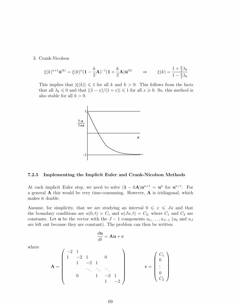
3. Crank-Nicolson
ξ(k)n+1u(k) = ξ(k)n(1 − h
2A)−1(1 +
h
2A)u(k) ⇒ ξ(k) =
1 + h2λk
1 − h2λk
This implies that |ξ(k)| 6 1 for all k and h > 0. This follows from the factsthat all λk 6 0 and that |(1 − x)/(1 + x)| 6 1 for all x > 0. So, this method isalso stable for all h > 0.
7.2.5 Implementing the Implicit Euler and Crank-Nicolson Methods
At each implicit Euler step, we need to solve (1 − hA)un+1 = un for un+1. Fora general A this would be very time-consuming. However, A is tridiagonal, whichmakes it doable.
Assume, for simplicity, that we are studying an interval 0 6 x 6 Ja and thatthe boundary conditions are u(0, t) = C1 and u(Ja, t) = C2, where C1 and C2 areconstants. Let u be the vector with the J − 1 components u1, . . . , uJ−1 (u0 and uJ
are left out because they are constant). The problem can then be written
du
dt= Au + c
where
A =
−2 11 −2 1 0
1 −2 1. . . . . . . . .
0 1 −2 11 −2
c =
C1
0...0C2
69

The (J − 1)× (J − 1)-matrix A is called tridiagonal because it has nonzero elementsonly in three bands along its diagonal. The matrix 1−hA is tridiagonal too, and thismakes it possible to solve the equation (1 − hA)x = y for x in O(J) operations, byGauss elimination. This figure illustrates how this is done for an arbitrary tridiagonalN × N -matrix:
b1 c1
a2 b2 c2
a3 b3 c3
. . . . . . . . .
−a2/b1
← →
b1 c1
0 b′2 = b2 − a2c1/b1 c2
a3 b3 c3
. . . . . . . . .
−a3/b′2
←→ . . . →
b1 c1
b′2 c2
b′3 c3
. . . . . .
b′N−1 cN−1
b′N
"
−cN−1/b′N
→ . . .
There are ≈ N steps “downwards” and ≈ N steps “upwards” and each step requiresO(1) operations, which makes the total cost O(N).
In the Crank-Nicolson method, there is also a tridiagonal system of equations to besolved at each step. The same method can be used in this case.
7.2.6 Higher Dimensions
So far, we have restricted ourselves to one-dimensional diffusion (d = 1). Formally, itis straightforward to extend these methods to higher d. To illustrate that, considerthe two-dimensional diffusion problem
∂u
∂t=
∂2u
∂x2+
∂2u
∂y2
70

with fixed boundary conditions, u = 0. Assume, for simplicity, that the region studiedis rectangular. We can then discretize x and y as follows.
xj = ja (j = 0, . . . , J)
yl = la (l = 0, . . . , L)
ujl(t) = u(xj, yl, t)
dujl
dt≈ uj+1l + uj−1l + ujl+1 + ujl−1 − 4ujl
a2
Put all “internal” (non-constant) ujl in a vector with a single index i, which may bedefined as i = (j − 1)(L − 1) + l − 1.
We can then write the discretized diffusion equation as
du
dt= Au (+ constant vector if there are nonzero boundary values)
The Crank-Nicholson method, for example, can be directly applied to this equation,which gives
un+1 = (1 − h2A)−1(1 + h
2A)un .
Formally, this looks precisely as before. However, the matrix A now has 5 bandsinstead of 3, which makes the problem computationally harder. The cost of thecalculation of un+1 scales linearly with the number of rows or columns of the matrixin this case too, but this number is larger, (J − 1) · (L− 1), and the prefactor in thisscaling law is higher when the number of bands is 5 instead of 3.
The Alternating Direction Implicit method (ADI)
ADI is a method that, like the Crank-Nicolson method, is second order in time andstable for all h > 0. The advantage of ADI compared to Crank-Nicolson is that it
71

works with tridiagonal matrices. This can be achieved by splitting the matrix A intotwo terms,
A = Ax + Ay ,
where Ax and Ay correspond to ∂2/∂x2 and ∂2/∂y2, respectively. Both Ax and Ay
are tridiagonal. To be able to take advantage of that, each ADI step is split into twosubsteps:
un+1/2 = un + h
2(Axu
n+1/2 + Ayun)
un+1 = un+1/2 + h2(Axu
n+1/2 + Ayun+1)
“implicit in x, explicit in y′′
“explicit in x, implicit in y′′
There are two equation systems to be solved, one for each substep, and they are bothtridiagonal,
(1 − h2Ax)u
n+1/2 = (1 + h2Ay)u
n
(1 − h2Ay)u
n+1 = (1 + h2Ax)u
n+1/2
The method can be summarized in one equation by eliminating un+1/2, which gives
un+1 = (1 − h2Ay)
−1(1 + h2Ax)(1 − h
2Ax)
−1(1 + h2Ay)u
n
7.3 The Poisson Equation
Consider the Poisson equation
∆u(x) = ∇ · ∇u(x) = −ρ(x) x ∈ Ω
with the boundary condition u(x) = f(x), x ∈ ∂Ω (∂Ω denotes the boundary of Ω).Such a condition that specifies u itself on the boundary (f is a given function) iscalled a Dirichlet boundary condition.
This boundary-value problem appears at different places in physics. An exampleis electrostatics. u is then the electrostatic potential and ρ the charge density (insuitable units).
Suppose we want to solve this problem by finite differencing. The problem is thentransformed into a linear algebra problem of the form Au = b, where A, as before,corresponds to ∆ and b is a vector that is determined by ρ and the function f in theboundary condition.
Solving this system of equations is, in principle, straightforward. The problem is thesize of the system; if, for example, we are in d = 2 and work with a 1000× 1000 grid,then there are 106 u components and 1012 elements in the matrix A. This makes itnecessary to make use of the fact that A is sparse (that is, only a tiny fraction of itselements are nonzero).
72

7.3.1 Relaxation Methods
A widely used strategy for solving the boundary value problem above is to let thesystem evolve in a fictitious time τ with diffusive dynamics. We then consider thediffusion problem
∂u
∂τ= ∆u + ρ x ∈ Ω, τ > 0
u = f x ∈ ∂Ω, τ > 0some initial condition τ = 0
where ρ and f are the same as in the original problem. In general, u will approacha stationary state as τ → ∞; that is, ∂u/∂τ → 0 as τ → ∞. This stationary state isthe desired solution.
Suppose we evolve u in τ by using a finite-difference method of the form
un+1 = Tun + constant vector .
The matrix T is called the iteration matrix. The convergence rate is governed by thespectral radius ρT of this matrix, defined by
ρT = maxeigenvalues λ of T
|λ| .
To see this, we first note that the desired solution must correspond to a fix point ofthe recursion formula. Denote this fix point by uf . The deviation from the fix pointsatisfies
un+1 − uf = T(un − uf) .
which implies that|un − uf | ∼ ρn
T n → ∞(unless the projection of u0 − uf onto the eigenvector with maximum |λ| happens tobe zero). This first of all shows that the method will converge if ρT < 1. We also seethat for the convergence to be fast, ρT should be as small as possible.
7.3.2 The Jacobi method
A simple relaxation method is the Jacobi method, which is obtained by using anEuler step in τ . The method is given by
un+1 = Tun + ρ ,
73

where the iteration matrix T = 1 + hA and the vector ρ represents the chargedensity ρ(x) (for simplicity, we assume that f = 0). As usual, the matrix A is ourapproximation of the Laplace operator ∆. It is the same as before.
Assume that we are in two dimensions and that the region Ω is a square,
Ω = (x, y); 0 6 x, y 6 Ja
It is then easy to find the eigenvalues and eigenvectors of A, which are given by
Av(kx,ky) = λkx,kyv(kx,ky) kx, ky = 1, . . . , J − 1
λkx,ky= − 4
a2
(
sin2 kxπ
2J+ sin2 kyπ
2J
)
v(kx,ky)jl = sin
jkxπ
Jsin
lkyπ
J
The eigenvalues of the iteration matrix T are given by
λTkx,ky
= 1 + hλkx,ky.
It is clear that λTkx,ky
6 1, since λkx,ky6 0. The lowest eigenvalue of T is
λTJ−1,J−1 = 1 + hλJ−1,J−1 ≈ 1 − 2
4h
a2.
This shows that in order to have ρT 6 1, we must take h 6 a2/4. In the Jacobimethod, one takes h = a2/4. With this choice, the time evolution is given by
un+1jl =
1
4(un
j+1l + unj−1l + un
jl+1 + unjl−1) +
a2
4ρjl .
To find ρT and thereby the convergence rate, we note that
max λTkx,ky
= 1 + hλ1,1 = 1 − 2 sin2 π
2J≈ 1 − π2
2J2
min λTkx,ky
= 1 + hλJ−1,J−1 = 1 − 2 sin2 (J − 1)π
2J= cos
(J − 1)π
J≈ −1 +
π2
2J2
So, ρT ≈ 1 − π2/2J2. The number of iterations, r, required to reduce the error by afactor 10−p satisfies
ρrT ∼ 10−p ⇒ r ≈ −p ln 10
ln ρT
≈ 2p ln 10
π2J2 .
Hence, the number of iterations scales quadratically with J . This makes the methodtoo slow to be of direct practical interest.
74

7.3.3 The Gauss-Seidel Method
This method is very similar to the Jacobi method. The only difference is that “new”u values are used as soon as they become available. This gives a slightly betterconvergence rate, but the scaling of the required number of iterations with systemsize remains quadratic.
The Gauss-Seidel method can be written as
un+1jl =
1
4(un
j+1l+ un+1j−1l↑
+unjl+1+ un+1
jl−1↑
) +a2
4ρjl
The Jacobi and Gauss-Seidel method are slow but important as starting points formore advanced methods.
Successive overrelaxation (SOR; see computer exercise 3) is based on the Gauss-Seidelmethod. It is almost as simple as the Gauss-Seidel method to implement, but muchmore efficient — the number of iterations needed scales as J rather than J2, providedthat the overrelaxation parameter ω is carefully chosen.
Multigrid methods (see NR) are more advanced. They are very efficient, but alsomore complicated than SOR to implement.
7.3.4 The Fourier Transform Method
Consider the boundary value problem
∂2u
∂x2+
∂2u
∂y2= −ρ 0 < x < X, 0 < y < Y
u(0, y) = u(X, y), u(x, 0) = u(x, Y ) periodic boundary conditionsu(0, 0) = u0
75

A very efficient method for this problem can be obtained by using Fourier decompo-sition:
u(x, y) =∞∑
kx=−∞
∞∑
ky=−∞u(kx, ky)e
2πi
„
kxxX
+kyy
Y
«
u (kx, ky) =1
XY
∫ X
0
dx
∫ Y
0
dyu(x, y)e−2πi
„
kxxX
+kyy
Y
«
Do the same for ρ(x, y). Insertion into the Poisson equation gives
−4π2[ (
kx
X
)2+
(ky
Y
)2 ]
u (kx, ky) = −ρ (kx, ky) ,
which is a simple algebraic equation for u, in place of the original differential equation.
This gives us a three-step “algorithm” for solving the given problem:
1. Transform ρ → ρ.
2. Calculate u(kx, ky) by using the algebraic equation above for all (kx, ky) 6= (0, 0).For kx = ky = 0, u is determined by the additional condition u(0, 0) = u0.
3. Transform u → u.
Numerically, these calculations are done using discrete Fourier transforms,
fn =1√N
N∑
k=1
fke2πikn
N fk =1√N
N∑
n=1
fne−2πikn
N
With the method of Fast Fourier Transform (FFT), the cost of a transform fn 7→ fk
(or vice versa) becomes ∼ N ln N rather than N2.
This makes this method very fast. However, it requires that the region considered isrectangular, which is a strong limitation (although the boundary conditions do nothave to be periodic).
7.4 Waves
The one-dimensional wave equation
∂2u
∂t2− v2∂2u
∂x2= 0
76

describes, for example, the transverse motion of a free string. This can be seen byconsidering a small string element dx. The string is assumed to be homogeneouswith a linear density ρ, so the mass of the small element is ρdx. Furthermore, it isassumed that the tension T is constant, and that the motion is “small” in the sensethat the angle θ in the figure below stays small. The equation for the transversemotion of the small element then is
ρdx∂2u
∂t2= T sin θ|x+dx − T sin θ|x ≈ T tan θ|x+dx − T tan θ|x ⇒
ρdx∂2u
∂t2≈ T
∂u
∂x
∣∣∣x+dx
− T∂u
∂x
∣∣∣x≈ Tdx
∂2u
∂x2⇒ ∂2u
∂t2≈ T
ρ
∂2u
∂x2(v =
√
T/ρ)
The one-dimensional wave equation can be solved by changing variables to ξ = x−vtand η = x + vt. The equation then becomes
∂2u
∂ξ∂η= 0 ⇒ u = f(ξ) + g(η) = f(x − vt) + g(x + vt) ,
where the functions f and g are determined by the initial values of u itself and thevelocity ∂u/∂t (the equation is second order in time). f(x−vt) and g(x+vt) representright- and left-moving waves, respectively (v > 0).
77

Instead of the wave equation, we will, for simplicity, consider
∂u
∂t+ v
∂u
∂x= 0 ,
which has right-moving solutions only; the same change of variables as before gives
∂u
∂η= 0 ⇒ u = f(ξ) = f(x − vt) .
It is instructive to solve this problem by separation of variables, which means thatwe write the solution as a superposition of solutions of the form u(x, y) = X(x)T (t).This ansatz gives
X ′(x)
X(x)= −1
v
T ′(t)
T (t)≡ ik = constant ⇒ X(x) ∝ eikx, T (t) ∝ e−ikvt ,
where the constant k must be real for X to remain bounded as x → ±∞. This showsthat uk(x, t) = ei(kx−ω(k)t), where ω(k) = kv, is a solution to the given equation forall real k. The general solution can be written as a continuous superposition of suchsolutions,
u(x, t) =1√2π
∫ ∞
−∞c(k)ei(kx−ω(k)t)dk ,
where c(k) is determined by initial data. Suppose a (right-moving) “wave packet” isexpressed in this way. The fact that ω(k) = kv implies that all plane-wave compo-nents uk of the wave packet have the same phase velocity (v). This in turn impliesthat the wave packet propagates without changing shape.
If the phase velocity vf = ω(k)/k were k dependent, then the shape of a wave packetwould change with time. This is called dispersion.
This may be further generalized by considering a complex ω(k) = Ω(k)−iγ(k), whereΩ and γ both are real. In this case, it can be shown (by using Parseval’s formula)that
∫ ∞
−∞|u(x, t)|2dx =
1
2π
∫ ∞
−∞
∣∣∣∣
∫ ∞
−∞c(k)ei(kx−ω(k)t)dk
∣∣∣∣
2
dx
=1
2π
∫ ∞
−∞dx dk dk′c(k)c(k′)ei(kx−ω(k)t)e−i(k′x−ω(k′)t)
=1
2π
∫ ∞
−∞dk dk′c(k)c(k′)ei(ω(k′)−ω(k))t)
∫ ∞
−∞dxeix(k−k′)
=
∫ ∞
−∞|c(k)|2e−2γ(k)tdk .
78

From this result we see that the normalization∫|u|2dx is preserved as long as ω is
real (γ = 0). If, on the other hand, γ > 0, the normalization integral decreases withtime. This is called damping.
7.4.1 Discrete waves
Let us now look at how to solve the equation ∂u/∂t = −v∂u/∂x by finite differencing.As usual, we put un
j = u(xj, tn), where xj = ja and tn = nh. For the space derivative,we use a central difference,
∂u
∂x
∣∣∣t=tn
=un
j+1 − unj−1
2a+ O(a2)
The Euler Method
With an Euler step in time, we get
un+1j − un
j
h= −v
unj+1 − un
j−1
2a⇒ un+1
j = unj − hv
2a(un
j+1 − unj−1)
To check the stability of the method, we make a von Neumann ansatz, unj = ξ(k)neikxj .
This gives
ξ(k) = 1 − hv
2a(eika − e−ika) = 1 − i
hv
asin ka ⇒
|ξ(k)|2 = 1 +
(hv
a
)2
sin2 ka > 1
showing that |unj | = |ξ(k)|n grows exponentially with n for all h > 0. So, this method,
which may not seem unreasonable, is a disaster — it is always unstable.
The Lax Method
The method above can be improved by a simple modification, which gives the so-called Lax method. The modification is that un
j is replaced by the average of unj+1
and unj−1. This gives
un+1j =
1
2(un
j+1 + unj−1) −
hv
2a(un
j+1 − unj−1) .
This time the ansatz unj = ξ(k)neikxj gives
ξ(k) =1
2(eika + e−ika) − hv
2a(eika − e−ika) = cos ka − i
hv
asin ka ,
and from the figure below it can be seen that |ξ(k)| 6 1 for all k if hv/a 6 1. So, themethod is stable if h 6 a/v. How does the discrete solution behave?
79

The k dependence of ξ(k) corresponds to an ω(k) given by
ξ(k) = e−iω(k)h = cos ka − ihv
asin ka .
If hv/a = 1, we see that hω = ka. So, ω = ka/h = kv, which happens to be theexact result.
If, on the other hand, hv/a < 1, then
|ξ|2 = e−2hγ = cos2 ka +
(hv
a
)2
sin2 ka < 1 .
This means that γ > 0, so the discrete solution is, in contrast to the exact one,damped. The damping is, however, small if ka is small. The real part Ω of ω satisfies
hΩ = arctan
((hv/a) sin ka
cos ka
)
≈ arctan hvk ≈ hvk
if ka is small. This shows that ω(k) for the discrete solution is approximately correctif the wavelength is much larger than a, so that ka ≪ 1. Short-wavelength modeshave large relative errors but are damped, so these errors do not destroy the long-wavelength properties of the solution.
The Leapfrog Method
The Lax method is first order in time and second order in space. A method that issecond order in time too can be obtained by using a central-difference approximationfor the time derivative, which gives
un+1j = un−1
j − vh
a
(un
j+1 − unj−1
).
80
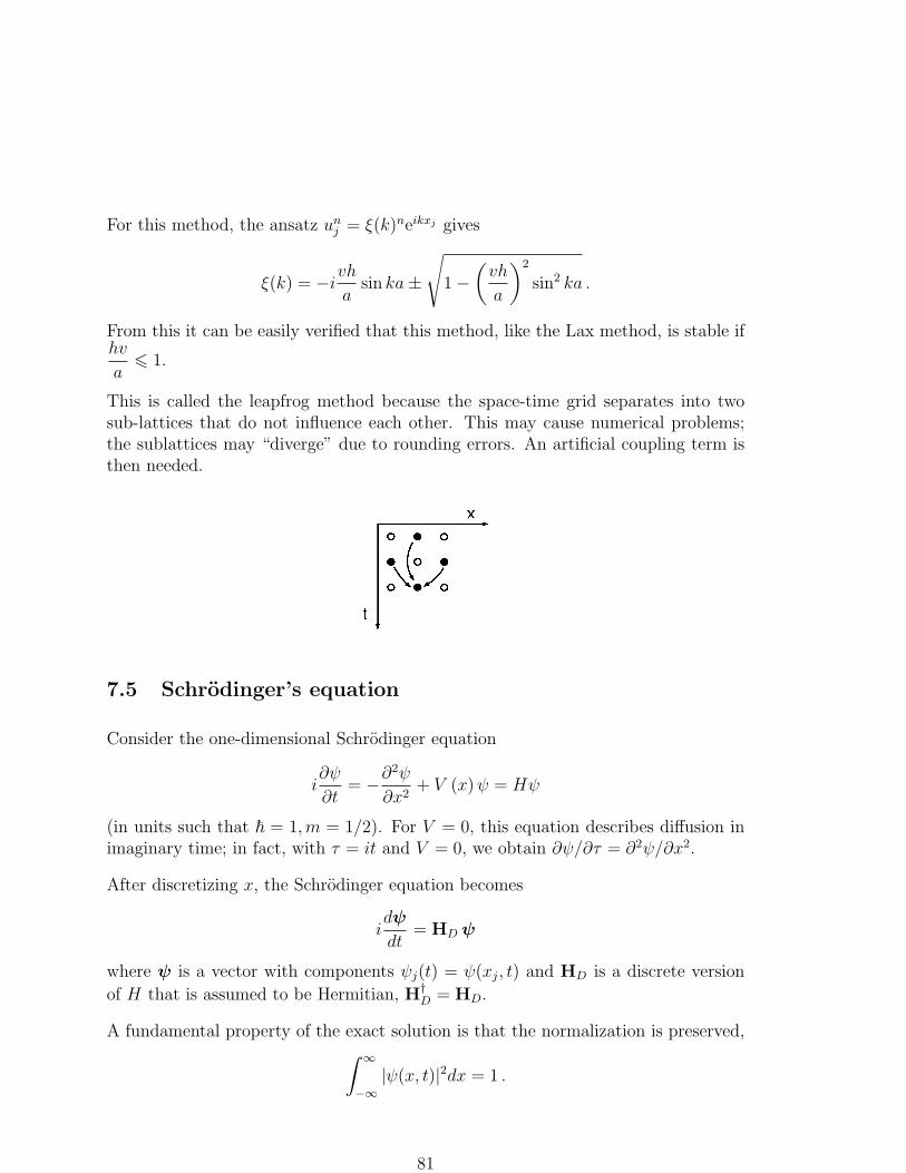
For this method, the ansatz unj = ξ(k)neikxj gives
ξ(k) = −ivh
asin ka ±
√
1 −(
vh
a
)2
sin2 ka .
From this it can be easily verified that this method, like the Lax method, is stable ifhv
a6 1.
This is called the leapfrog method because the space-time grid separates into twosub-lattices that do not influence each other. This may cause numerical problems;the sublattices may “diverge” due to rounding errors. An artificial coupling term isthen needed.
7.5 Schrodinger’s equation
Consider the one-dimensional Schrodinger equation
i∂ψ
∂t= −∂2ψ
∂x2+ V (x) ψ = Hψ
(in units such that ~ = 1,m = 1/2). For V = 0, this equation describes diffusion inimaginary time; in fact, with τ = it and V = 0, we obtain ∂ψ/∂τ = ∂2ψ/∂x2.
After discretizing x, the Schrodinger equation becomes
idψ
dt= HD ψ
where ψ is a vector with components ψj(t) = ψ(xj, t) and HD is a discrete version
of H that is assumed to be Hermitian, H†D = HD.
A fundamental property of the exact solution is that the normalization is preserved,∫ ∞
−∞|ψ(x, t)|2dx = 1 .
81

Does this remains true after discretizing x? The discrete analog is
d
dt(ψ†ψ) =
(1
iHDψ
)†ψ +
1
iψ†HDψ = 0 .
The eigenvalues EI of HD are real, since HD is Hermitian. Denote the eigenvectorsby ψI ,
HDψI = EIψI .
The eigenvectors may be assumed to be orthonormal.
Let us now consider three possible ways of discretizing t.
1. The explicit Euler method gives
ψn+1 = ψn − ihHDψn = Tψn ,
where the iteration matrix T = 1 − ihHD. The eigenvalues of T are λI =1 − ihEI and satisfies |λI | > 1 for all I. Suppose now
ψ0 =∑
I
cIψI ⇒ ψn =∑
I
cIλnI ψI .
From the fact that the eigenvectors are orthonormal, it follows that the nor-malization
|ψn|2 = ψn†ψn =∑
I
|cI |2λ2nI .
This implies that |ψn|2 is not constant, but increases exponentially with n (forlarge n).
2. With an implicit Euler step instead, we obtain
ψn+1 = ψn − ihHDψn+1 ⇒ ψn+1 = Tψn
with T = (1 + ihHD)−1. The eigenvalues of T are this time given by λI =1/(1 + ihEI), so |λI | 6 1 for all I. It follows that |ψn|2 decreases steadily withn.
3. Finally, we consider the Crank-Nicholson method (or trapezoidal rule),
ψn+1 = ψn +h
2(−iHDψn − iHDψn+1) ,
which can be written ψn+1 = Tψn with
T =
(
1 + ih
2HD
)−1 (
1 − ih
2HD
)
.
82

The eigenvalues of this T are
λI =1 − i
h
2EI
1 + ih
2EI
.
Since λI is a ratio between two numbers that are the complex conjugates of eachother, it follows that |λI | = 1 (for all I), and therefore that |ψn|2 is constant.So, the Crank-Nicolson method has the advantage that the normalization ispreserved.
8 Appendix: χ2 Minimization
[NR 15.5]
When discussing minimization, we mentioned the Newton method for root finding.This method can be used to solve the equation system ∇f(x) = 0, and thereby findthe minimum of a given cost function f . Usually, this is an impractical method, butit is useful for function fitting.
Suppose we want to fit a set of data points (xi, yi) with errors σi, i = 1, . . . , N , to afunction y(x; a), where a = (a1, . . . , aM) are parameters (M < N). This is usuallydone by minimizing
χ2(a) =N∑
i=1
(yi − y(xi, a)
σi
)2
with respect to a.
If the function y depends linearly on the parameters ai, this amounts to solvinga relatively simple linear algebra problem. To see this, assume that y is a linearcombination of some basis functions ϕk,
y(x; a) =M∑
k=1
akϕk(x) .
χ2 can then be expressed as
χ2(a) =N∑
i=1
(
yi −∑M
k=1 akϕk(xi)
σi
)2
=N∑
i=1
(
bi −M∑
k=1
Aikak
)2
= |b − Aa|2 ,
83

where A is the matrix with elements Aik = ϕk(xi)/σi and b is the vector withcomponents bi = yi/σi. Putting ∇χ2(a) = 0, we get a linear equation system for theparameters ai,
ATAa = ATb .
These equations are called the normal equations and can be solved, for example, bysingular value decomposition (SVD; see NR 2.6 and p. 676).
If y is a non-linear function of the parameters ai, it is necessary to take a differentapproach. A popular choice is to use the Levenberg-Marquardt method, which canbe thought of as a combination of steepest descent and the Newton method. In theLevenberg-Marquardt method, we need the gradient of χ2,
∂χ2
∂ak
= −2N∑
i=1
yi − y(xi, a)
σ2i
∂y(xi, a)
∂ak
as well as the Hessian,
∂2χ2
∂ak∂al
= 2N∑
i=1
1
σ2i
[∂y(xi, a)
∂ak
∂y(xi, a)
∂al
− (yi − y(xi, a))∂2y(xi, a)
∂ak∂al
]
.
Here the last term should be small if we are near the minimum and the fit is good(it vanishes if y depends linearly on the parameters). For convenience, this term isneglected, which does not affect the final ak values and which gives
∂2χ2
∂ak∂al
≈ Akl = 2N∑
i=1
1
σ2i
∂y(xi, a)
∂ak
∂y(xi, a)
∂al
.
Put
βk = −1
2
∂χ2
∂ak
αkl =1
2Akl δak = a′
k − ak .
In this notation, a steepest descent step has the form δak = constant · βk. TheLevenberg-Marquardt method does not use a proper steepest descent step but rather
δak =1
λαkk
βk ,
where λ is a parameter (see below) and αkk is introduced because the different com-ponents ak may behave very differently; dividing by αkk makes sense dimensionally.Note that αkk is guaranteed to be positive because we are using the simplified versionof the Hessian.
84

A Newton step can be written as
a′ = a − A(a)−1∇χ2(a) ⇒∑
l
αklδal = βk .
The Levenberg-Marquardt method can be seen as an elegant way to interpolate be-tween these two types of step, by changing the parameter λ. This is achieved byconsidering
∑
kl
αklδal = βk where αkl =
αkk(1 + λ) k = lαkl k 6= l
For λ → 0, this becomes a Newton step, because the matrices αkl and αkl are thesame in this limit. For large λ, on the other hand, we get a modified steepest descentstep, because the diagonal elements dominate the matrix αkl.
The idea is to start with a large λ which gives a steepest descent-like step, and thengradually decrease λ as we get closer to the minimum, so that the step becomes moreand more Newton-like.
Schematically, the algorithm can be written as:
1. Pick some initial a and a large λ.
2. Solve the equation system for δa and calculate χ2(a + δa).
3. If χ2(a + δa) < χ2(a), update a to anew = a + δa, decrease λ, and continue at2. If χ2(a + δa) ≥ χ2(a), increase λ (decrease the step size) and go back to 2without changing a.
Iterate till some stopping criterion is fulfilled.
85