lecture notes for fast fourier transform - boston …straubin/scicomp_2011/fftlecture.pdfthe...
TRANSCRIPT

Lecture Notes for Fast Fourier Transform
CS227-Scientific Computing
November 16, 2011

Part I: What it Does

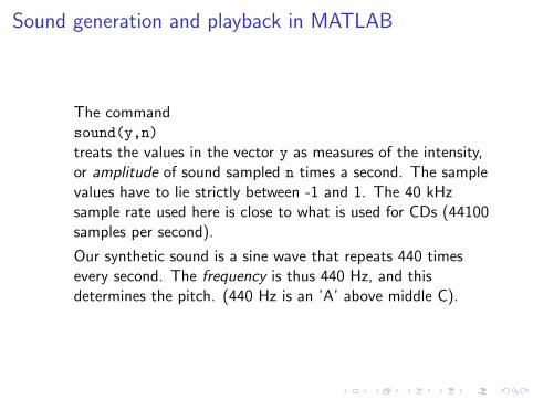
Sound generation and playback in MATLAB
Try the following commands:
>> t=linspace(0,1,40000);>> y1=cos(2*pi*440*t);>> sound(y1,40000)
Sound generation and playback in MATLAB
The commandsound(y,n)treats the values in the vector y as measures of the intensity,or amplitude of sound sampled n times a second. The samplevalues have to lie strictly between -1 and 1. The 40 kHzsample rate used here is close to what is used for CDs (44100samples per second).
Our synthetic sound is a sine wave that repeats 440 timesevery second. The frequency is thus 440 Hz, and thisdetermines the pitch. (440 Hz is an ’A’ above middle C).

Superimposing sinusoids
Now let’s add another, higher-pitched, tone on top of thisone, and listen to the result:
>> y2=sin(2*pi*660*t);>> y=(y1+y2)/2;>> sound(y,40000)
Note that we average the two sets of amplitudes so that thesample values don’t go outside the range (−1, 1).
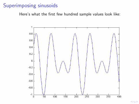
Superimposing sinusoids
Here’s what the first few hundred sample values look like:

Superimposing sinusoids
Just for fun, let’s add a little noise:
>> z=0.7*y+0.1*randn(1,40000);

Extracting frequencies from the signal
The plots above display the signal as amplitude vs. time. Butthere is also a way to display the data as amplitude vs.frequency. For this we use the MATLAB function fft. Thisstands for Fast Fourier Transform.
>> trans = fft(z);>> trans(1:3)
ans =
-19.0792 7.4440 + 1.3015i 14.2555 +13.1185i
fft returns a vector of complex numbers of the same size asits argument.

Extracting frequencies from the signal
Let’s plot the magnitudes of these complex numbers:
trans=fft(z);plot(1:40000,abs(trans));
It’s not very revealing, but let’s zoom in for a closeup:

Extracting frequencies from the signal
The big spikes are at 440 Hz and 660 Hz, right where we putthem! The added noise makes small contributions at a lot ofdifferent frequencies, so it appears like grass growing at thebottom of the picture.

Extracting frequencies from the signal
You’ll note that in the original figure, there are two identicalspikes at the far right end of the plot. The Fourier transformis symmetric about a frequency equal to half the samplingrate. You can view the information in the right-hand half asartifacts of the mathematical method used to produce thetransform. (We’ll see shortly why this is.) The real frequencyinformation is in the left-hand half.
If you weighted the two sinusoidal components differently, thiswould be reflected in the differing height of the spikes.

Part II: How Does this Work (and what’swith the complex numbers?)

Some basics about the complex numbers
We represent the point (a, b) in the plane as a + bi , acomplex number.
If we declare i · i = −1, then we can add and multiply any twopoints in the plane. Addition is just ordinary vector addition,but to multiply two such complex numbers, we multiply theirmagnitudes (i.e., their lengths) and add the angles that theymake with the positive x-axis.
Why is this? Because a point a distance of r from the originmaking an angle of θ with the positive x-axis has coordinates(r cos θ, r sin θ).

So to get the multiplication to work out right with i2 = −1we would have to have:
(r1 cos θ1 + i · r1 sin θ1) · (r2 cos θ2 + i · r2 sin θ2) =
r1r2((cos θ1 cos θ2 − sin θ1 sin θ2) + i(cos θ1 sin θ2 + sin θ1 cos θ2)) =
r1r2(cos(θ1 + θ2) + i(sin(θ1 + θ2)).
Amazingly, it all works out. Multiplication is associative anddistributive, every nonzero element has a multiplicativeinverse, etc.
The multiplicative inverse of z = x + iy is x−iyx2+y2 = z̄
|z|2 .
z̄ = x − iy is called the complex conjugate of z .

Complex Multiplication

Complex Exponentiation
But there is more amazement to come. Imagine a particlemoving counterclockwise around the unit circle with a speedof 1 unit per second. It starts at the point(1, 0) = 1 + 0 · i = 1, so at time t its position isz(t) = cos t + i · sin t. This is our basic picture for thesimplest kind of periodic motion–for sinusoids. This has aperiod of 2π seconds and a fequency of 1
2π hertz.
The particle’s velocity vector at time t points in a directionperpendicular to z(t) and has a magnitude of 1. It’s just z(t)rotated 90 degrees counterclockwise; that is, the velocity isi · z(t).
Complex Exponentiation
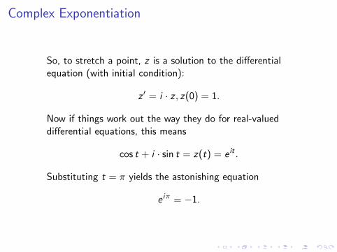
So, to stretch a point, z is a solution to the differentialequation (with initial condition):
z ′ = i · z , z(0) = 1.
Now if things work out the way they do for real-valueddifferential equations, this means
cos t + i · sin t = z(t) = e it .
Substituting t = π yields the astonishing equation
e iπ = −1.

The Fourier Transform matrix
Let us choose an integer n > 0, and let ω = e2πin . Note that
ω−1 = ω̄.
The numbers 1, ω, ω2, . . . , ωn−1 are the n distinct nth roots of1. Geometrically, they are the vertices of a regular n-sidedpolygon inscribed inside the unit circle, with one vertex at thepoint (1, 0).
Physically, you can think of the numbers 1, ω, ω2, . . . as thepositions of a point at times 0, 1
n ,2n , etc. This represents
sinusoidal motion with a period of 1 and a frequency of 1cycle per time unit.
Similarly, the sequence 1, ω2, ω4, . . . represents sinusoidalmotion with twice the frequency (2 cycles per time unit);1, ω3, ω6, . . . motion with frequency of 3 cycles per time unit,etc.
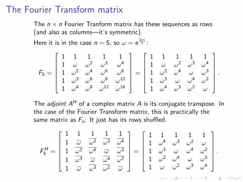
The Fourier Transform matrix
The n × n Fourier Tranform matrix has these sequences as rows(and also as columns—it’s symmetric).
Here it is in the case n = 5, so ω = e2πi
5 :
F5 =
1 1 1 1 11 ω ω2 ω3 ω4
1 ω2 ω4 ω6 ω8
1 ω3 ω6 ω9 ω12
1 ω4 ω8 ω12 ω16
=
1 1 1 1 11 ω ω2 ω3 ω4
1 ω2 ω4 ω ω3
1 ω3 ω ω4 ω2
1 ω4 ω3 ω2 ω
.The adjoint AH of a complex matrix A is its conjugate transpose. Inthe case of the Fourier Transform matrix, this is practically thesame matrix as Fn: It just has its rows shuffled.
FH5 =
1 1 1 1 1
1 ω ω2 ω3 ω4
1 ω2 ω4 ω ω3
1 ω3 ω ω4 ω2
1 ω ω3 ω2 ω
=
1 1 1 1 11 ω4 ω3 ω2 ω1 ω3 ω ω4 ω2
1 ω2 ω4 ω ω3
1 ω ω2 ω3 ω4
.

The Fourier Transform matrix
The magic is that FHn is (almost) the same as F−1
n . (There’s anadditional constant factor.)
To see why, let’s take the dot product of column j of Fn withcolumn k of FH
n , We get
1 + ω(j−k) + ω2(j−k) + · · ·+ ω(n−1)(j−k).
We can use a little trick to show this sum is equal to 0. It’s justthe identity
xn − 1 = (x − 1)(1 + x + · · ·+ xn−1).
If we substitute x = ω(j−k), the left-hand side is 1-1= 0. However, ifj 6= k , then x 6= 1, so the second factor on the right-hand side is 0.
On the other hand, if j = k then every term in the dot product is 1,so the sum is equal to n. Thus we have
Fn · FHn = FH
n · F = nI .
The Fourier Transform
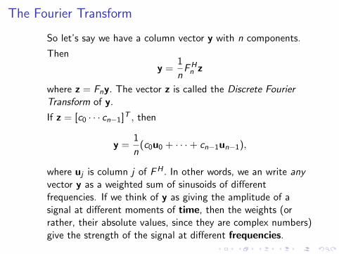
So let’s say we have a column vector y with n components.
Then
y =1
nFH
n z
where z = Fny. The vector z is called the Discrete FourierTransform of y.
If z = [c0 · · · cn−1]T , then
y =1
n(c0u0 + · · ·+ cn−1un−1),
where uj is column j of FH . In other words, we an write anyvector y as a weighted sum of sinusoids of differentfrequencies. If we think of y as giving the amplitude of asignal at different moments of time, then the weights (orrather, their absolute values, since they are complex numbers)give the strength of the signal at different frequencies.

The Fourier Transform
Let’s give a few examples of this. Suppose first n = 100, so
that ω = e2πi100 .
Consider the vector
y = (1, cos2π
10, cos
2 · 2π10
, . . . , cos99 · 2πi
10).
We can write
y =1
2((1, ω10, ω20, . . . , ω99·10) + (1, ω−10, ω−20, . . . , ω−99·10))

The Fourier Transform
From what we observed earlier,
F100y
has the value n in the 11th and the 91st components. (Thisaccounts for the symmetry we observed in the transform.)
If we apply the transform instead to the vector
y′ = (1, cos2π
11, cos
2 · 2π11
, . . . , cos99 · 2πi
11),
then F100y′ no longer exhibits the massive cancellation we sawin computing F100y. But it is close, which is what we observedin our original example.

Part III: The Discrete Fourier Transform inMATLAB

The Fourier Transform
The Discrete Fourier Transform is a terrific tool for signalprocessing (along with many, many other applications).However the catch is that to compute Fny in the obvious way,we have to perform n2 complex multiplications. If we aretransforming a vector with 40,000 components (1 second ofsampled audio on a CD), we need 1.6 billion suchmultiplications.
In 1965. James Cooley and John Tukey published analgorithm for computing this that used only n · log2 nmultiplications. With n = 40, 000, this is about 600 thousandmultiplications, which is almost three thousand times fasterthan the obvious method.
The so-called Fast Fourier Transform is not a differenttransform from the DFT, it’s just a different way ofcomputing it.

MATLAB fft and ifft
In MATLAB you just typez = fft(y)to get a complex vector z that is the DFT of y. The inversetransform, which, as we have seen, is almost the same thing, isgotten byy = ifft(z).

Example: Extracting periodic information from climatedata
The Fourier transform was used to analyze 28 years of hourlytemperature data, in degrees Fahrenheit, from a weatherstation in Colorado. You can see the seasonal variation, withlow temperatures in the winter (the data start January 1,1976) and high temperatures in the summer.
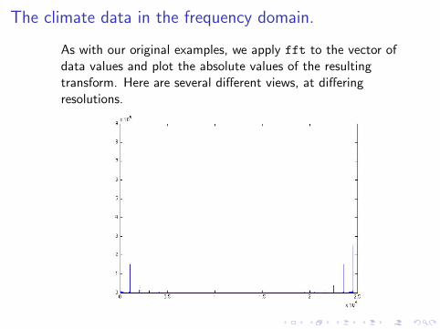
The climate data in the frequency domain.
As with our original examples, we apply fft to the vector ofdata values and plot the absolute values of the resultingtransform. Here are several different views, at differingresolutions.

The climate data in the frequency domain.
The full transform exhibits the kind of symmetry we alwayssee when we transform real-valued data.
The general rule is this: if we number the components of thetransform z0, . . . , zn−1, then for j > 0,
zj = z̄n−j .
This means|zj | = |zn−j |,
which accounts for the symmetry when we plot it.

The climate data in the frequency domain.

The climate data in the frequency domain.
The closeup of the left-hand end of the plot shows the largeDC component at x = 1. This gives no information abouttemperature data.
The next large spike occurs at x = 29. Since we have toadjust by 1 (because MATLAB indexes vectors starting at 0),this corresponds to a frequency of 28. But 28 what? It is 28cycles per the complete sampling interval—in this case, 28cycles per 28 years, or 1 cycle per year. This is the annualtemperature fluctuation.
What about the smaller spikes to the right? The next two ofthese occur at x = 57 and x = 85, corresponding tofrequencies of 56 and 84 cycles in the interval, or 2 cycles peryear and 3 cycles per year. Such ‘overtones’ at integermultiples of the fundamental frequency are common in thistransformed data.

The climate data in the frequency domain.

The climate data in the frequency domain.
When we zoom out we see spikes at x ≈ 10230 and smallmultiples thereof. What is this?
The entire sampling interval contains 245448 samples.245448 = 10227× 24, so this represents exactly 10227 days.
Thus these spikes correspond to a frequency of one cycle perday.
The Fourier transform shows very clearly the dailytemperature fluctuation superimposed on the yearly cycle.