lecture notes - arxiv.org notes ws 2009/2010 max lein september 3, ... 8.5 semiclassical limit ......
TRANSCRIPT
Weyl Quantization and SemiclassicsLecture Notes
WS 2009/2010
Max Lein∗
September 3, 2010
Zentrum MathematikLehrstuhl M5
Boltzmannstr. 385747 Garching
arX
iv:1
009.
0444
v1 [
mat
h-ph
] 1
Sep
201
0

Acknowledgements
I would like to thank Herbert Spohn for his encouragement, support and cutting the redtape. Chapters 3 and 4 follow closely his ‘Quantendynamik’ from 2005. Furthermorethe physical arguments presented in Chpater 7 to arrive at the proper formulation of thesemiclassical limit (which I feel is the most important part) in is based on his lecture.
Furthermore, I would like to express my gratitude towards Martin Fürst and DavidSattlegger who were very helpful in improving the lecture.
iii

iv

Contents
1 Introduction 1
2 Physical Frameworks 52.1 Hamiltonian framework of classical mechanics . . . . . . . . . . . . . . . . . . 52.2 Quantum mechanics . . . . . . . . . . . . . . . . . . . . . . . . . . . . . . . . . . 132.3 Comparison of the two frameworks . . . . . . . . . . . . . . . . . . . . . . . . . 192.4 Properties of quantizations . . . . . . . . . . . . . . . . . . . . . . . . . . . . . . 20
3 Hilbert spaces 233.1 Prototypical Hilbert spaces: L2(Rd) and `2(Zd) . . . . . . . . . . . . . . . . . . 233.2 Abstract Hilbert spaces . . . . . . . . . . . . . . . . . . . . . . . . . . . . . . . . . 243.3 Orthonormal bases and orthogonal subspaces . . . . . . . . . . . . . . . . . . . 273.4 Subspaces (⊕) and product spaces (⊗) . . . . . . . . . . . . . . . . . . . . . . . 333.5 Linear functionals, dual space and weak convergence . . . . . . . . . . . . . . 353.6 Important facts on Lp(Rd) . . . . . . . . . . . . . . . . . . . . . . . . . . . . . . . 40
4 Linear operators 434.1 Bounded operators . . . . . . . . . . . . . . . . . . . . . . . . . . . . . . . . . . . 434.2 Adjoint operator . . . . . . . . . . . . . . . . . . . . . . . . . . . . . . . . . . . . . 464.3 Unitary operators . . . . . . . . . . . . . . . . . . . . . . . . . . . . . . . . . . . . 484.4 Selfadjoint operators . . . . . . . . . . . . . . . . . . . . . . . . . . . . . . . . . . 55
5 Schwartz functions and tempered distributions 575.1 Schwartz functions . . . . . . . . . . . . . . . . . . . . . . . . . . . . . . . . . . . 575.2 Tempered distributions . . . . . . . . . . . . . . . . . . . . . . . . . . . . . . . . . 65
6 Weyl calculus 716.1 The Weyl system . . . . . . . . . . . . . . . . . . . . . . . . . . . . . . . . . . . . . 726.2 Weyl quantization . . . . . . . . . . . . . . . . . . . . . . . . . . . . . . . . . . . . 746.3 The Wigner transform . . . . . . . . . . . . . . . . . . . . . . . . . . . . . . . . . 786.4 Weyl product . . . . . . . . . . . . . . . . . . . . . . . . . . . . . . . . . . . . . . . 866.5 Asymptotics . . . . . . . . . . . . . . . . . . . . . . . . . . . . . . . . . . . . . . . 916.6 Application: Diagonalization of the Dirac equation . . . . . . . . . . . . . . . 95
v

Contents
7 The semiclassical limit 99
8 Theory of multiscale systems 1118.1 Physics of molecules: the Born-Oppenheimer approximation . . . . . . . . . 1118.2 The adiabatic trinity . . . . . . . . . . . . . . . . . . . . . . . . . . . . . . . . . . 1188.3 Intermezzo: Weyl calculus for operator-valued functions . . . . . . . . . . . . 1228.4 Effective quantum dynamics: adiabatic decoupling to all orders . . . . . . . 123
8.4.1 Construction of the projection . . . . . . . . . . . . . . . . . . . . . . . . 1248.4.2 Construction of the intertwining unitary . . . . . . . . . . . . . . . . . 1268.4.3 The effective hamiltonian . . . . . . . . . . . . . . . . . . . . . . . . . . 1278.4.4 Effective Dynamics . . . . . . . . . . . . . . . . . . . . . . . . . . . . . . . 129
8.5 Semiclassical limit . . . . . . . . . . . . . . . . . . . . . . . . . . . . . . . . . . . . 131
vi

1 Introduction
This lecture will elaborate on what a quantization is. If classical phase space, i. e. thespace of possible positions and momenta, is T ∗Rd
x∼= Rd
x ×Rdp , we give a concrete solution.
Roughly speaking, we generalize Dirac’s prescription to replace x by “multiplication withx ,”
( xϕ)(x) := x ϕ(x), ϕ ∈ L2(Rd),
and momentum by a “derivative with respect to x”
(pϕ)(x) :=−iħh∇xϕ(x), ϕ ∈ L2(Rd)∩C 1(Rd).
Dirac’s recipe only works if we are quantizing functions of x or p and their linear combi-nations, e. g. H(x , p) = 1
2mp2+V (x) becomes H = H( x , p) =− ħh2
2m∆x+V ( x), and it needs
to be supplemented with an “operator ordering prescription:” what is the quantization ofx · p? Possible solutions are
x · p, p · x = x · p− iħh idL2 , 12
x · p+ p · x
,
all of which are different operators and the first two are not even symmetric (= hermitian).Choosing an operator ordering is necessary, because x and p do not commute,
i[pl , x j] = ħhδl j .
The physical constant ħh has a fixed value and units and it measures the “degree of non-commutativity” of position and momentum. On the other hand, can we find the functionwhose quantization is, say, x · p =
∑dl=1 x l pl? One way to look at it is to find a product ]ħh
which emulates the operator product on the level of functions, i. e.
d∑
l=1
Øx l]ħhpl =d∑
l=1
x l pl .
On the one hand, this product must inherit the non-commutativity of the operator product,but on the other, if “ħh is small,” x l]pl should be approximately given by x l pl . One ofthe major reasons to study ]ħh is that we can use it to derive corrections in perturbation
1
1 Introduction
expansions: if we can find an expansion of the product ]ħh in ħh, we can “expand the operatorproduct:”
f g =Õf ]ħhg =∞∑
n=0
ħhnÙ( f ]ħhg)(n) + small error
We will make all of the above mathematically rigorous in this lecture and explain thesymbols properly. This idea was first proposed by Littlejohn and Weigert [LW93] (whoare theoretical physicists) and used both in a mathematically rigorous fashion and in the-oretical physics to derive currents in crystals that are subjected to electromagnetic fields[PST03a], piezocurrents [PST06, Lei05], guiding center motion of particles in electro-magnetic fields [Mü99], the non- and semirelativistic limit of the Dirac equation [FL08]and many others.
The second main point of this lecture is the semiclassical limit (“ħh → 0”): for ħh = 0, pand x commute. However, a priori it is not at all clear how and why this implies classicalbehavior. Let H(x , p) = 1
2mp2+ V (x) be a classical hamiltonian. If we start at t = 0 at the
point (x0, p0) in phase space, Hamilton’s equations of motion
x =+∇pH = pm
p =−∇x H =−∇x V
with initial conditions (x0, p0) determine a unique classical trajectory
x(t), p(t)
. Thequantum dynamics of a particle whose initial state is described by the wave function ψ0
is given by the Schrödinger equation,
iħh∂
∂ tψħh(t) = Hψħh(t) =
− 12m(−iħh∇x)
2 + V ( x)
ψħh(t), ψħh(0) =ψ0 ∈ L2(Rd). (1.1)
If in order to “take the semiclassical ħh → 0,” we naïvely set ħh = 0 in the Schrödingerequation, we get the unintelligible equation
0= V ( x)ψ0(t)
which implies trivial dynamics. The reason is that the actual solution requires a bit morethought. There are simple ansätze such as WKB functions, coherent states and otherwave packet approaches1, but this suggests that only special (“good”) initial states havea good semiclassical limit. First of all, why should nature “choose” such rather specialinitial conditions? Wave packet approaches are usually based on the Ehrenfest theorem
1A wave packet is a sharply peaked wave function whose envelope function varies slowly, just like in the caseof a WKB function. The center of the wave packet is interpreted as “semiclassical position” and the time-derivative of this center gives the classical velocity.
2
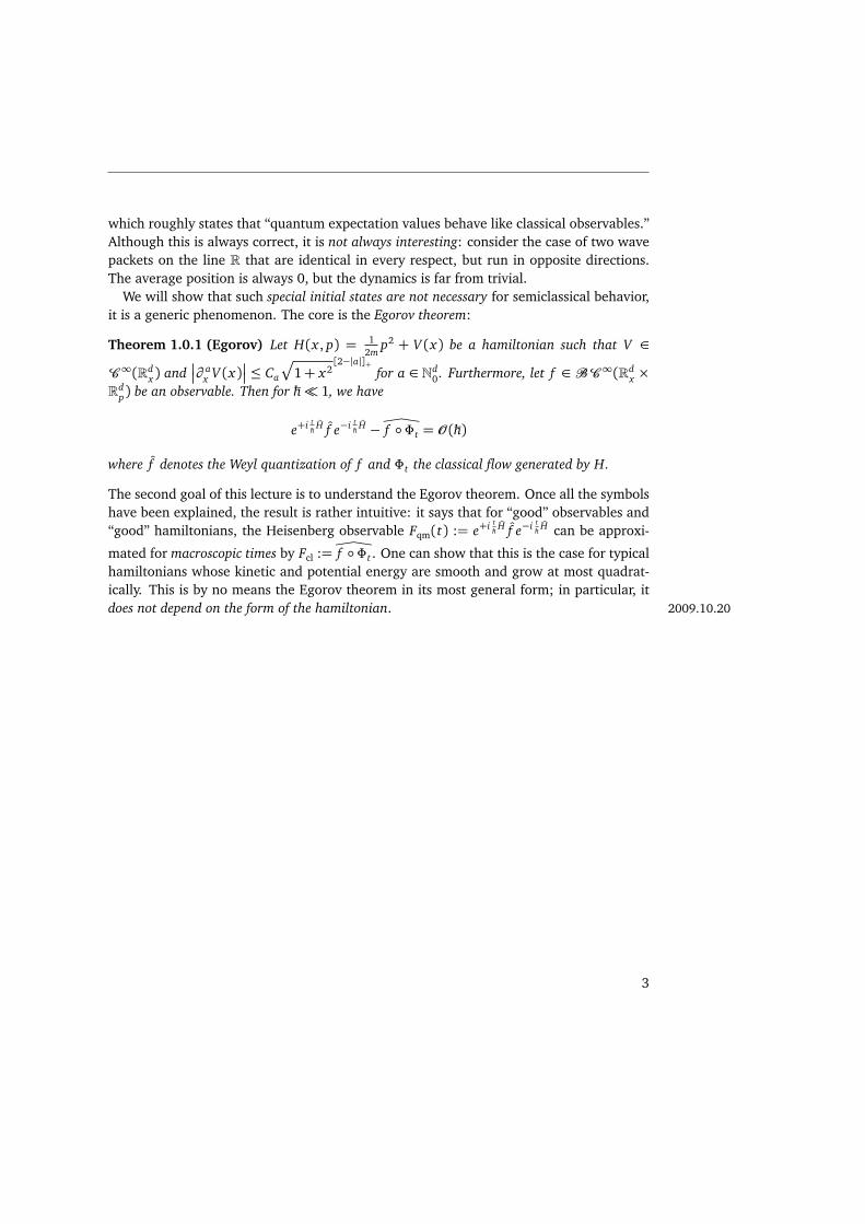
which roughly states that “quantum expectation values behave like classical observables.”Although this is always correct, it is not always interesting: consider the case of two wavepackets on the line R that are identical in every respect, but run in opposite directions.The average position is always 0, but the dynamics is far from trivial.
We will show that such special initial states are not necessary for semiclassical behavior,it is a generic phenomenon. The core is the Egorov theorem:
Theorem 1.0.1 (Egorov) Let H(x , p) = 12m
p2 + V (x) be a hamiltonian such that V ∈
C∞(Rdx) and
∂ ax V (x)
≤ Ca
p
1+ x2[2−|a|]+
for a ∈ Nd0 . Furthermore, let f ∈ BC∞(Rd
x ×Rd
p) be an observable. Then for ħh 1, we have
e+i tħh H f e−i t
ħh H −Øf Φt = O (ħh)
where f denotes the Weyl quantization of f and Φt the classical flow generated by H.
The second goal of this lecture is to understand the Egorov theorem. Once all the symbolshave been explained, the result is rather intuitive: it says that for “good” observables and“good” hamiltonians, the Heisenberg observable Fqm(t) := e+i t
ħh H f e−i tħh H can be approxi-
mated for macroscopic times by Fcl :=Øf Φt . One can show that this is the case for typicalhamiltonians whose kinetic and potential energy are smooth and grow at most quadrat-ically. This is by no means the Egorov theorem in its most general form; in particular, itdoes not depend on the form of the hamiltonian. 2009.10.20
3

1 Introduction
4

2 Physical Frameworks
Understanding of quantization requires knowledge of classical and quantum mechanics. Aquantization procedure is not merely a method to “consistently assign operators on L2(Rd)to functions on phase space,” but rather a collection of procedures. A nice overview of thetwo frameworks can be found in the first few sections of chapter 5 in [Wal08] and we willgive a condensed account here: physical theories consist roughly of three parts:
(i) A state space: states describe the current configuration of the system and need to beencoded in a mathematical structure.
(ii) Observables: they represent quantities physicists would like to measure. Related tothis is the idea of spectrum as the set of possible outcomes of measurements as wellas expectation values (if ones deals with distributions of states).
(iii) An evolution equation: usually, one is interested in the time evolution of states aswell as observables. As energy is the observable conjugate to time, energy functionsgenerate time evolution.
2.1 Hamiltonian framework of classical mechanics
For simplicity, we only treat classical mechanics of a spinless point particle moving in Rd ,for the more general theory, we refer to [MR99, Arn89]. In any standard lecture onclassical mechanics, at least two points of views are covered: lagrangian and hamiltonianmechanics.
We will only treat hamiltonian mechanics here: the dynamics is generated by the so-called hamilton function H : Rd
x × Rdp −→ R which describes the energy of the system
for a given configuration. Here, Rdx ×R
dp is also known as phase space. Since only energy
differences are measurable, the hamiltonian H ′ := H + E0, E0 ∈ R, generates the samedynamics as H. This is obvious from the hamiltonian equations of motion,
x(t) = +∇pH
x(t), p(t)
(2.1)
p(t) =−∇x H
x(t), p(t)
,
5

2 Physical Frameworks
which can be rewritten in matrix notation as
J
x(t)p(t)
:=
0 −idRd
+idRd 0
x(t)p(t)
=
∇x
∇p
H
x(t), p(t)
. (2.2)
The matrix J appearing on the left-hand side is often called symplectic form and leadsto a geometric point of view of classical mechanics. For fixed initial condition (x0, p0) ∈Rd
x ×Rdp at time t0 = 0, i. e. initial position and momentum, the hamiltonian flow
Φ : Rt ×Rdx ×R
dp −→ Rd
x ×Rdp (2.3)
maps (x0, p0) onto the trajectory which solves the hamiltonian equations of motion,
Φt(x0, p0) =
x(t), p(t)
,
x(0), p(0)
= (x0, p0).
If the flow exists for all t ∈ Rt , it has the following nice properties: for all t, t ′ ∈ Rt and(x0, p0) ∈ Rd
x ×Rdp , we have
(i) Φt
Φt ′(x0, p0)
= Φt+t ′(x0, p0),
(ii) Φ0(x0, p0) = (x0, p0), and
(iii) Φt
Φ−t(x0, p0)
= Φt−t(x0, p0) = (x0, p0).
Mathematically, this means Φ is a group action of Rt (with respect to time translations) onphase space Rd
x ×Rdp . This is a fancy way of saying:
(i) If we first evolve for time t and then for time t ′, this is the same as evolving for timet + t ′.
(ii) If we do not evolve at all in time, nothing changes.
(iii) The system can be evolved forwards or backwards in time.
The existence of the flow is usually proven via the Theorem of Picard and Lindelöf. Itholds in much broader generality and is no easier to prove if we specialize to X = (x , p)and R2d = Rd
x ×Rdp .
Theorem 2.1.1 (Picard-Lindelöf) Let F be a continuous vector field, F ∈ C (U ,Rn), U ⊆Rn open, which defines a system of differential equations,
X = F(X ). (2.4)
Assume for a certain initial condition X0 ∈ U there exists a ball Bρ(X0) :=
X ∈ Rn | |X −X0| < ρ
⊆ U, ρ > 0, such that F is Lipschitz on Bρ(X0), i. e. there exists L > 0 whichsatisfies
F(X )− F(X ′)
≤ L
X − X ′
6

2.1 Hamiltonian framework of classical mechanics
for all X , X ′ ∈ Bρ(X0). Then the initial value problem, equation (2.4) with X (0) = X0, has aunique solution t 7→ X (t) for times |t| ≤ T := min
ρ/Vmax, 1/2L
where the maximal velocityis defined as Vmax := supX∈Bρ(X0)|F(X )|.
Multiplying the hamiltonian equations of motion (2.2) by the inverse of the symplecticform, we get the vector field F explicitly in terms of the gradients of H with respect to xand p.
Proof We only sketch the proof here since it is part of the standard course on analysis(for physicists) or differential equations (for mathematicians). It consists of three steps:
We can rewrite the initial value problem equation (2.4) with X (0) = X0 as
X (t) = X0 +
∫ t
0
ds F(X (s))
This equation can be solved iteratively: we define X0(t) := X0 and the n+ 1th iterationXn+1(t) :=
P(Xn)
(t) in terms of the so-called Picard map
P(Xn)
(t) := X0 +
∫ t
0
ds F(Xn(t)).
If t ∈ [−T,+T] and T > 0 is chosen to be small enough, P :X −→X is a contraction onthe space of trajectories which start at X0,
X :=n
Y ∈ C
[−T,+T], Bρ(X0)
Y (0) = X0
o
.
X is a complete metric space if we use
d(Y, Z) := supt∈[−T,+T]
Y (t)− Z(t)
Y, Z ∈ X
to measure distances between trajectories. A map P : X −→ X is a contraction if for allY, Z there exists C < 1 such that
d
P(Y ), P(Z)
≤ C d(Y, Z).
If the Picard iteration is a contraction on X , since it is complete, the sequence (Xn) con-verges to the unqiue solution of (2.4) X = P(X ) by the Banach fix point theorem.
To show that P is really a contraction, we need to treat both possible choices of T : thefirst, T ≤ ρ/Vmax implies that the trajectory cannot leave the ball Bρ(X0). For any Y ∈ X ,we have
P(Y )− X0
=
∫ t
0
ds F(Y (s))
≤ t Vmax ≤ T Vmax < ρ.
7

2 Physical Frameworks
The second condition, T ≤ 1/2L, together with the Lipschitz property ensure that it is alsoa contraction with C = 1/2: for any Y, Z ∈ X , we have
d
P(Y ), P(Z)
= supt∈[−T,+T]
∫ t
0
ds
F(Y )
(t)−
F(Z)
(t)
≤ T L supt∈[−T,+T]
Y (t)− Z(t)
≤ 12L
L d(Y, Z) = 12d(Y, Z)
This concludes the proof.
Corrolary 2.1.2 If the vector field F satisfies the Lipschitz condition globally, i. e. there existsL > 0 such that
F(X )− F(X ′)
≤ L
X − X ′
holds for all X , X ′ ∈ Rn, then t 7→ Φt(X0) exists globally for all t ∈ Rt and X0 ∈ Rn.
Proof For every X0 ∈ Rn, we can solve the initial value problem at least for |t| ≤ 1/2L.Since
F(X0)
≤
F(0)
+ L
X0
implies that if we choose our ball large enough, i. e. for any ρ >
X0
+|F(0)|/L, the condition|t| ≤ ρ/Vmax is automatically satisfied,
ρ
Vmax≥
ρ
|F(0)|+ L(
X0
+ρ)≥
1
2L.
Hence, we can patch local solutions together using the group property Φt Φt ′ = Φt+t ′ ofthe flow to obtain global solutions.
Another important fact is that the flow Φ inherits the smoothness of the vector field whichgenerates it.2009.10.21
Theorem 2.1.3 Assume the vector field F is k times continuously differentiable, F ∈ C k(U ,Rn),U ⊆ Rn. Then the flow Φ associated to (2.4) is also k times continuously differentiable,i. e. Φ ∈ C k[−T,+T]× V, U
where V ⊂ U is suitable.
Proof We refer to Chapter 3, Section 7.3 in [Arn92].
The above results immediately apply to the hamiltonian equations of motion:
Corrolary 2.1.4 Let H = 12m
p2 + V (x) be the hamiltonian which generates the dynamicsaccording to equation (2.2) such that ∇x V satisfies a global Lipschitz condition
∇x V (x)−∇x V (x ′)
≤ L
x − x ′
∀x , x ′ ∈ Rdx .
Then the hamiltonian flow Φ exists for all t ∈ Rt .
8

2.1 Hamiltonian framework of classical mechanics
Classical states Pure states in classical mechanics are simply points in phase space: apoint particle’s state at time t is characterized by its position x(t) and momentum p(t).More generally, one can consider distributions of initial conditions which are relevant instatistical mechanics, for instance.
Definition 2.1.5 (Classical states) A classical state is a probability measure µ on phasespace, that is a positive Borel measure1 which is normed to 1,
µ(U)≥ 0 for all Borel sets U ⊆ Rdx ×R
dp
µ(Rdx ×R
dp) = 1.
Pure states are point measures, i. e. if (x0, p0) ∈ Rdx ×R
dp , then the associated pure state is
given by µ(x0,p0)(·) := δ(x0,p0)(·) = δ(· − (x0, p0)).2
Observables Observables f such as position, momentum, angular momentum and en-ergy are smooth functions on phase space with values in R, f ∈ C∞(Rd
x ×Rdp ,R). If we
compose observables with the flow, we can work with time-evolved observables
f (t) := f Φt : Rdx ×R
dp −→ R
where Φ is the flow generated by some suitable hamiltonian H. If
x(t), p(t)
is the tra-jectory associated to the initial conditions (x0, p0), then
f (t)
(x0, p0) = f
Φt(x0, p0)
=f
x(t), p(t)
gives the value of the observable at time t. This is analogous to the Heisen-berg picture in quantum mechanics: observables are evolved in time and states stay con-stant. The possible outcomes of measurements is given by the
Definition 2.1.6 (Spectrum of an observable) The spectrum of a classical observables, i. e. theset of possible outcomes of measurements, is given by
spec f := f (Rdx ×R
dp) = im f .
If we are given a classical state µ, then the expected value Eµ of an observable f for thedistribution of initial conditions µ is given by
Eµ
f (t)
:=
∫
Rdx×R
dp
dµ(x , p) f
Φt(x , p)
=
∫
Rdx×R
dp
dµ
Φ−t(x , p)
f (x , p)
=Eµ(t)( f ).
1Unfortunately we do not have time to define Borel sets and Borel measures in this context. We refer theinterested reader to chapter 1 of [LL01]. Essentially, a Borel measure assigns a “volume” to “nice” sets,i. e. Borel sets.
2Here, δ is the Dirac distribution which we will consider in detail in Chapter 5.
9
2 Physical Frameworks
The right-hand side corresponds to the Schrödinger picture where states are evolved intime and not observables: the time-evolved state µ(t) associated to µ is defined by µ(t) :=µ Φ−t .
Time evolution Now to the dynamics: we have already defined the time-evolved observ-able f (t). Which equation generates its time evolution?
Proposition 2.1.7 Let f ∈ C∞(Rdx ×R
dp ,R) be an observable and Φ the hamiltonian flow
which solves the equations of motion (2.2) associated to a hamiltonian H ∈ C∞(Rdx×R
dp ,R)
which we assume to exist globally in time for all (x0, p0) ∈ Rdx ×R
dp . Then
d
dtf (t) =
H, f (t)
(2.5)
holds where
f , g
:=∑d
l=1
∂plf ∂x l
g − ∂x lf ∂pl
g
is the so-called Poisson bracket.
Proof Theorem 2.1.3 implies the smoothness of the flow from the smoothness of thehamiltonian. This means f (t) ∈ C∞(Rd
x × Rdp ,R) is again a classical observable. By as-
sumption, all initial conditions lead to trajectories that exist globally in time.3 For (x0, p0),we compute the time derivative of f (t) to be
d
dtf (t)
(x0, p0) =d
dtf
x(t), p(t)
=d∑
l=1
∂x lf Φt(x0, p0) x l(t) + ∂pl
f Φt(x0, p0) pl(t)
∗=
d∑
l=1
∂x lf Φt(x0, p0)∂pl
H Φt(x0, p0)+
+ ∂plf Φt(x0, p0)
−∂x lH Φt(x0, p0)
=
H(t), f (t)
.
In the step marked with ∗, we have inserted the hamiltonian equations of motion. Com-pared to equation (2.5), we have H instead of H(t) as argument in the Poisson bracket.However, by setting f (t) = H(t) in the above equation, we see that energy is a conservedquantity,
d
dtH(t) =
H(t), H(t)
= 0.
Hence, we can replace H(t) by H in the Poisson bracket with f and obtain equation (2.5).3A slightly more sophisticated argument shows that the Proposition holds if the hamiltonian flow exists only
locally in time.
10

2.1 Hamiltonian framework of classical mechanics
The proof immediately leads to the notion of conserved quantity:
Definition 2.1.8 (Conserved quantity/constant of motion) An observable f ∈ C∞(Rdx×
Rdp ,R) which is invariant under the flow Φ generated by the hamiltonian H ∈ C∞(Rd
x ×Rd
p ,R), i. e.
f (t) = f (0),
or equivalently satisfies
d
dtf (t) =
H, f (t)
= 0,
is called conserved quantity or constant of motion.
As is very often in physics and mathematics, we have completed the circle: starting fromthe hamiltonian equations of motion, we have proven that the time evolution of observ-ables is given by the Poisson bracket. Alternatively, we could have started by postulating
d
dtf (t) =
H, f (t)
for observables and we would have arrived at the hamiltonian equations of motion byplugging in x and p as observables. Another important fact is Liouville’s Theorem whichstates that the hamiltonian flow preserves phase space volume:
Theorem 2.1.9 (Liouville) The hamiltonian vector field is divergence free, i. e. the hamil-tonian flow preserves volume in phase space of bounded subsets V of Rd
x ×Rdp with smooth
boundary ∂ V . In particular, the functional determinant of the flow is constant and equal to
det
DΦt(x , p)
= 1
for all t ∈ Rt and (x , p) ∈ Rdx ×R
dp .
Remark 2.1.10 We will need a fact from the theory of dynamical systems: if Φt is theflow associated to a differential equation X = F(X ) with F ∈ C 1(Rd , Rd), then
d
dtDΦt(X ) = DF(X )DΦt(X ), DΦt
t=0 = idRd ,
holds for the differential of the flow. As a consequence, one can prove
d
dt
det DΦt(X )
= tr
DF
Φt(X )
det
DΦt(X )
= div F
Φt(X )
det
DΦt(X )
,
and det
DΦt
t=0 = 1. We refer to [Dre07, Chapter 1.6] for details and proofs.
11

2 Physical Frameworks
Figure 2.1: Phase space volume is preserved under the hamiltonian flow.
Proof Let H be the hamiltonian which generates the flow Φt . Let us denote the hamilto-nian vector field by
XH =
+∇pH−∇x H
.
Then a direct calculation yields
div XH =d∑
l=1
∂x l
+∂plH
+ ∂pl
−∂x lH
= 0
and the hamiltonian vector field is divergence free. This implies the hamiltonian flow Φt
preserves volumes in phase space: let V ⊆ Rdx ×R
dp be a bounded region in phase space (a
Borel subset) with smooth boundary. Then for all −T ≤ t ≤ T for which the flow exists,we have
d
dtVol
Φt(V )
=d
dt
∫
Φt (V )
dx dp
=d
dt
∫
V
dx ′ dp′ det
DΦt(x′, p′)
.
Since V is bounded, we can bound det
DΦt
and its time derivative uniformly. Thus, caninterchange integration and differentiation and apply Remark 2.1.10,
d
dt
∫
V
dx ′ dp′ det
DΦt(x′, p′)
=
∫
V
dx ′ dp′d
dtdet
DΦt(x′, p′)
=
∫
V
dx ′ dp′ div XH
Φt(x′, p′)
︸ ︷︷ ︸
=0
det
DΦt(x′, p′)
= 0.
12
2.2 Quantum mechanics
Hence ddt
Vol (V ) = 0 and the hamiltonian flow conserves phase space volume. The func-tional determinant of the flow is constant as the time derivative vanishes,
d
dtdet
DΦt(x′, p′)
= 0,
and equal to 1,
det
DΦt(x′, p′)
t=0 = det idRdx×R
dp= 1.
This concludes the proof.
With a different proof relying on alternating multilinear forms, the requirements on V canbe lifted, see e. g. [KS04, Satz 29.3 and Satz 29.5].
Corrolary 2.1.11 Let µ be a state on phase space Rdx ×R
dp and Φt the flow generated by a
hamiltonian H ∈ C∞(Rdx ×R
dp) which we assume to exist for |t| ≤ T where 0 < T ≤ ∞ is
suitable. Then µ(t) is again a state.
Proof Since Φt is continuous, it is also measurable. Thus µ(t) = µ Φ−t is also a Borelmeasure on Rd
x ×Rdp (Φ−t exists by assumption on t). In fact, Φt is a diffeomorphism on
phase space. Liouville’s theorem not only ensures that the measure µ(t) remains positive,but also that it is normalized to 1: let U ⊆ Rd
x ×Rdp be a Borel subset. Then we conclude
µ(t)
(U) =
∫
U
d
µ(t)
(x , p) =
∫
U
dµ
Φ−t(x , p)
=
∫
Φ−t (U)
dµ(x , p)≥ 0
where we have used the positivity of µ and the fact that Φ−t(U) is again a Borel set bycontinuity of Φ−t . If we set U = Rd
x×Rdp and use the fact that the flow is a diffeomorphism,
we see that Rdx×R
dp is mapped onto itself, Φ−t(Rd
x×Rdp) = R
dx×R
dp , and the normalization
of µ leads to
µ(t)
(Rdx ×R
dp) =
∫
Φ−t (Rdx×R
dp)
dµ(x , p) =
∫
Rdx×R
dp
dµ(x , p) = 1
This concludes the proof.
2.2 Quantum mechanics
While position and momentum characterize the state of a classical particle, both are notsimultaneously measurable with arbitrary precision in a quantum system. This is forbidden
13
2 Physical Frameworks
by Heisenberg’s uncertainty principle,
∆ψ x∆ψ p ≥ħh2
,
where
∆ψ x :=p
Varψ( x) :=p
ψ, ( x − ⟨ψ, xψ⟩)2ψ
and∆ψ p :=p
Var(p) are the standard deviations of position and momentum with respectto the state ψ. They quantify how sharply the wave function ψ is peaked in positionand momentum space. Either we can pinpoint the location with increased precision (re-duce the standard deviation ∆ψ x) or measure the particle’s momentum more accurately(reduce ∆ψ p). In contrast, the variance (and thus the standard deviation) of a classical2009.10.22observable with respect to a pure state vanishes,
Varδ(x0,p0)( f ) :=Eδ(x0,p0)
( f −Eδ(x0,p0)( f ))2)
= Eδ(x0,p0)( f 2)−Eδ(x0,p0)
( f )2
= f 2(x0, p0)− f (x0, p0)2 = 0.
Quantum particles simultaneously have wave and particle character: the Schrödingerequation
iħh∂
∂ tψ(t) = Hψ(t), ψ(t) ∈ L2(Rd),ψ(0) =ψ0,
is structurally very similar to a wave equation. H is the so-called hamilton operator (hamil-tonian for short) and is typically given by
H =1
2m(−iħh∇x)
2 + V ( x).
Here m > 0 is the mass of the particle and V the potential it has been subjected to. Thephysical constant ħh relates the energy of a particle with the associated wavelength andhas units of [energy · time].
Pure states are described by wave functions, i. e. complex-valued, square integrablefunctions
ψ ∈ L2(Rd) :=n
ψ : Rd −→ C
ψ measurable,
∫
Rd
dx
ψ(x)
2<∞
o
/∼ . (2.6)
L2(Rd) with the usual scalar product
φ,ψ
:=
∫
Rd
dx φ(x)∗ψ(x) (2.7)
14

2.2 Quantum mechanics
and norm
ψ
:=p
ψ,ψ
is the prototype of a Hilbert space. ∼ means we identify twofunctions if they agree almost everywhere. We will discuss this space in much more detailin Chapter 3 and we focus on the physical content rather than mathematics. In physicstext books, one usually encounters the the bra-ket notation: here
ψ
is a state and
x |ψ
is ψ(x). The scalar product of φ,ψ ∈ L2(Rd) is denoted by
φ|ψ
and corresponds to
φ,ψ
. Although bra-ket notation can be ambiguous, it is sometimes useful and in factused in mathematics every once in a while.
Physically,
ψ(x , t)
2is interpreted as the probability to measure a particle at time t in
(an infinitesimally small box located in) location x . If we are interested in the probabilitythat we can measure a particle in a region Λ ⊆ Rd , we have to integrate
ψ(x , t)
2over
Λ,
P(X (t) ∈ Λ) =∫
Λ
dx
ψ(x , t)
2. (2.8)
If we want to interpret
ψ
2as probability density, the wave function has to be normalized,
i. e.
ψ
=
È
∫
Rd
dx
ψ(x)
2= 1.
This point of view is called Born rule:
ψ
2could either be a mass or charge density – or
a probability density. To settle this, physicists have performed the double slit experimentwith an electron source of low flux. If
ψ
2were a density, one would see the whole
interference pattern building up slowly. Instead, one measures “single impacts” of elec-trons and the result is similar to the data obtained from experiments in statistics (e. g. theDalton board). Hence, we speak of particles.
Quantum observables Quantities that can be measured are represented by symmetric(hermitian) operators A on the Hilbert space (typically L2(Rd)), i. e. special linear maps
A : D(A)⊆ L2(Rd)−→ L2(Rd).
Here, D(A) is the domain of the operator since typical observables are not defined forall ψ ∈ L2(Rd). This is not a mathematical subtlety with no physical content, quite thecontrary: consider the observabble energy, typically given by
H =1
2m(−iħh∇x)
2 + V ( x),
then states in the domain
D(H) :=n
ψ ∈ L2(Rd)
Hψ ∈ L2(Rd)o
⊆ L2(Rd)
15
2 Physical Frameworks
are those of finite energy. For all ψ in the domain of the hamiltonian D(H) ⊆ L2(Rd), theexpectation value
ψ, Hψ
<∞
is bounded. Well-defined observables have domains that are dense in L2(Rd). Similarly,states in the domain D( x l) of the lth component of the position operator are those thatare “localized in a finite region” in the sense of expectation values.
Physically, results of measurements are real which is reflected in the selfadjointness ofoperators,4
H∗ = H.
The spectrum σ(H) ⊆ R is the set of all possible outcomes of measurements. Unfortu-nately, we cannot define the spectrum now, but we will do so in Chapter 4.1.
Typically one “guesses” quantum observables from classical observables: in d = 3, theangular momentum operator is given by
L = x ∧ p = x ∧ (−iħh∇x).
In the simplest case, one uses Dirac’s recipe (replace x by x and p by p = −iħh∇x) on theclassical observable angular momentum L(x , p) = x ∧ p. In other words, many quantumobservables are obtained as quantizations of classical observables: examples are position,momentum and energy. Moreover, the interpretation of, say, the angular momentum op-erator as angular momentum is taken from classical mechanics. This is an indication howimportant quantizations are conceptually.
In the definition of the domain, we have already used the definition of expectationvalue: the expectation value of an observable A with respect to a state ψ (which weassume to be normalized,
ψ
= 1) is given by
Eψ(A) :=
ψ, Aψ
. (2.9)
The expectation value is finite if the state ψ is in the domain D(A). The Born rule ofquantum mechanics tells us that if we repeat an experiment measuring the observable Amany times for a particle that is prepared in the state ψ each time, the statistical averagecalculated according to the relative frequencies converges to the expectation value Eψ(A).
Hence, quantum observables, selfadjoint operators on Hilbert spaces, are bookkeepingdevices that have two components:
(i) a set of possible outcomes of measurements, the spectrum σ(A), and
(ii) statistics, i. e. how often a possible outcome occurs.
If for two quantum observables A and B have the same spectrum and statistics, they havethe chance of being “equivalent.”
4A symmetric operator is selfadjoint if H∗ = H and D(H∗) = D(H), see Chapter 4.4.
16

2.2 Quantum mechanics
Quantum states Pure states are wave functions ψ ∈ L2(Rd), or rather, wave functionsup to a total phase: just like one can measure only energy differences, only phase shifts areaccessible to measurements. Hence, one can think of pure states as orthogonal projections
Pψ := |ψ⟩⟨ψ|= ⟨ψ, ·⟩ψ.
if ψ is normalized to 1,
ψ
= 1. Here, one can see the elegance of bra-ket notation vs.the notation that is “mathematically proper.” A generalization of this concept are densityoperators ρ (often called density matrices): density matrices are defined via the trace. If ρis a suitable linear operator and ϕnn∈N and orthonormal basis of L2(Rd), then we define
tr ρ :=∑
n∈N⟨ϕn, ρϕn⟩.
One can easily check that this definition is independent of the choice of basis and we willshow this in a later chapter. Clearly, Pψ has trace 1 and it is also positive in the sense that
ϕ, Pψϕ
≥ 0
for all ϕ ∈ L2(Rd). This is also the good definition for quantum states:
Definition 2.2.1 (Quantum state) A quantum state (or density operator/matrix) ρ is apositive operator of trace 1, i. e.
ψ, ρψ
≥ 0,
tr ρ = 1, ∀ψ ∈ L2(Rd).
If ρ is also an orthogonal projection, i. e. ρ2 = ρ, it is a pure state.5 Otherwise ρ is a mixedstate.
Example Letψ j ∈ L2(Rd) be two wave functions normalized to 1. Then for any 0< α < 1
ρ = αPψ1+ (1−α)Pψ2
= α|ψ1⟩⟨ψ1|+ (1−α)|ψ2⟩⟨ψ2|
is a mixed state as
ρ2 = α2|ψ1⟩⟨ψ1|+ (1−α)2|ψ2⟩⟨ψ2|++α(1−α)
|ψ1⟩⟨ψ1||ψ2⟩⟨ψ2|+ |ψ2⟩⟨ψ2||ψ1⟩⟨ψ1|
6= ρ.
Even if ψ1 and ψ2 are orthogonal to each other, since α2 6= α and similarly (1− α)2 6=(1−α), ρ cannot be a projection. Nevertheless, it is a state since tr ρ = α+ (1−α) = 1.Keep in mind that ρ does not project on αψ1 + (1−α)ψ2!
5Note that the condition tr ρ = 1 implies that ρ is a bounded operator while the positivity implies the selfad-jointness. Hence, if ρ is a projection, i. e. ρ2 = ρ, it is automatically also an orthogonal projection.
17

2 Physical Frameworks
Time evolution The time evolution is determined through the Schrödinger equation,
iħh∂
∂ tψ(t) = Hψ(t), ψ(t) ∈ L2(Rd), ψ(0) =ψ0,
ψ0
= 1. (2.10)
Alternatively, one can write ψ(t) = U(t)ψ0 with U(0) = idL2 . Then, we have
iħh∂
∂ tU(t) = HU(t), U(0) = idL2 .
If H were a number, one would immediately use the ansatz
U(t) = e−i tħh H (2.11)
as solution to the Schrödinger equation. If H is a selfadjoint operator, this is still true, buttakes a lot of work to justify rigorously if the domain of H is not all of L2(Rd) (the case ofunbounded operators, the generic case).
As has already been mentioned, we can evolve either states or observables in time andone speaks of the Schrödinger or Heisenberg picture, respectively. In the Schrödingerpicture, states evolve according to
ψ(t) = U(t)ψ0
while observables remain fixed. Conversely, in the Heisenberg picture, states are keptfixed in time and observables evolve according to
A(t) := U(t)∗ AU(t) = e+i tħh H Ae−i t
ħh H . (2.12)
Heisenberg observables satisfy
d
dtA(t) =
i
ħh
H, A(t)
(2.13)
which can be checked by plugging in the definition of A(t) and elementary formal manipu-2009.10.27lations. It is no coincidence that this equation looks structurally similar to equation (2.5)!
As a last point, we mention the conservation of probability: ifψ(t) solves the Schrödingerequation for some selfadjoint H, then we can check at least formally that the time evolu-tion is unitary and thus preserves probability,
d
dt
ψ(t)
2=
d
dt
ψ(t),ψ(t)
= 1
iħh Hψ(t),ψ(t)
+
ψ(t), 1iħh Hψ(t)
=i
ħh
ψ(t), H∗ψ(t)
−
ψ(t), Hψ(t)
=i
ħh
ψ(t), (H∗ − H)ψ(t)
= 0.
18
2.3 Comparison of the two frameworks
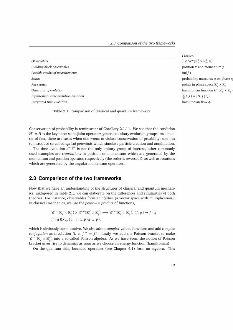
Classical Quantum
Observables f ∈ C∞(Rdx ×R
dp ,R) selfadjoint operators acting on Hilbert space L2(Rd)
Building block observables position x and momentum p position x and momentum p operators
Possible results of measurements im( f ) σ(A)
States probability measures µ on phase space Rdx ×R
dp density operators ρ on L2(Rd)
Pure states points in phase space Rdx ×R
dp wave functions ψ ∈ L2(Rd)
Generator of evolution hamiltonian function H : Rdx ×R
dp −→ R hamiltonian operator H
Infinitesimal time evolution equation ddt
f (t) = H, f (t) ddt
A(t) = iħh[H, A(t)]
Integrated time evolution hamiltonian flow φt e+i tħh H e−i t
ħh H
Table 2.1: Comparison of classical and quantum framework
Conservation of probability is reminiscent of Corollary 2.1.11. We see that the conditionH∗ = H is the key here: selfadjoint operators generate unitary evolution groups. As a mat-ter of fact, there are cases when one wants to violate conservation of proability: one hasto introduce so-called optical potentials which simulate particle creation and annihilation.
The time evolution e−i tħh H is not the only unitary group of interest, other commonly
used examples are translations in position or momentum which are generated by themomentum and position operator, respectively (the order is reversed!), as well as rotationswhich are generated by the angular momentum operators.
2.3 Comparison of the two frameworks
Now that we have an understanding of the structures of classical and quantum mechan-ics, juxtaposed in Table 2.1, we can elaborate on the differences and similarities of boththeories. For instance, observables form an algebra (a vector space with multiplication):in classical mechanics, we use the pointwise product of functions,
· :C∞(Rdx ×R
dp)×C
∞(Rdx ×R
dp)−→C
∞(Rdx ×R
dp), ( f , g) 7→ f · g
( f · g)(x , p) := f (x , p) g(x , p),
which is obviously commutative. We also admit complex-valued functions and add complexconjugation as involution (i. e. f ∗∗ = f ). Lastly, we add the Poisson bracket to makeC∞(Rd
x × Rdp) into a so-called Poisson algebra. As we have seen, the notion of Poisson
bracket gives rise to dynamics as soon as we choose an energy function (hamiltonian).On the quantum side, bounded operators (see Chapter 4.1) form an algebra. This
19
2 Physical Frameworks
algebra is non-commutative, i. e.
A · B 6= B · A.
Exactly this is what makes quantum mechanics different. Taking adjoints is the involutionhere and the commutator plays the role of the Poisson bracket. Again, once a hamiltonian(operator) is chosen, the dynamics of Heisenberg observables A(t) is determined by thecommutator of the A(t) with the hamiltonian H. If an operator commutes with the hamil-tonian, it is a constant of motion. This is in analogy with Definition 2.1.8 where a classicalobservable is a constant of motion if and only if its Poisson bracket with the hamiltonian(function) vanishes.
2.4 Properties of quantizations
Quantization is a problem of theoretical and mathematical physics, not a problem of na-ture. Quantum mechanics is simply more fundamental than classical mechanics and thereason we can guess the correct quantum mechanics comes from the fact that most ob-servables we are interested are macroscopic and have a good semiclassical limit. In a way,quantization is going backwards again. That is the reason why not every quantum observ-able has a classical analog. Spin, for instance, is purely a quantum mechanical conceptwith no semiclassical limit.
Since quantum mechanics is more deep and classical mechanics emerges as an approx-imation under certain conditions, there should be “more” quantum observables than clas-sical observables (although it is usually not possible to qualify what we mean by “more,”the frameworks and constructions are too different). In the simplest case, we start with analgebra of classical observables and “quantize them,” i. e. we associate them to operatorson a Hilbert space in a systematic fashion. Although this is what most people think is aquantization, we emphasize that this is only part of what really is a consistent quantizationprocedure.
Let us call the quantization map Op which promotes suitable functions on phase spaceto operators on L2(Rd). A number of requirements on Op seem natural:
Linearity The map Op should be linear, i. e. for two classical observables f , g ∈ Acl takenfrom the algebra of classical observables and α,β ∈ C, we should have
Op
α f + β g
= αOp( f ) + βOp(g) ∈ Aqm.
Here, Aqm is an algebra of quantum observables.
20
2.4 Properties of quantizations
Compatibility with involution Op should intertwine complex conjugation and taking ad-joints, i. e. for all f ∈ Acl
Op( f ∗) =Op( f )∗ ∈ Aqm.
Products The two products cannot be equivalent: the operator product is noncommuta-tive and hence for general f , g ∈ Acl
Op( f · g) 6=Op( f ) ·Op(g).
Instead, for suitable functions f , g, we can define a non-commutative product ] on the levelof functions on phase space such that
Op( f ]g) :=Op( f ) ·Op(g) ∈ Aqm.
A priori it is not at all clear whether f ]g ∈ Acl.
Poisson bracket and commutator Roughly, Poisson bracket and commutators play simi-lar roles and thus are analogs of one another,
f , g
¡i
ħh
Op( f ),Op(g)
.
Just like with the product, the quantization of the Poisson bracket usually does not coin-cide with with 1/iħh times the commutator. 2009.10.28
Small parameters One of the most important (and potentially confusing) aspects of thesemiclassical limit is the question of the small parameter. Planck’s constant ħh is a physicalconstant, i. e. its value is fixed and it has units. Any good small parameter should nothave units, e. g. the fine structure constant α ' 1/137 is a good small parameter. Hence,we cannot take the limit ħh→ 0. Other interpretations of the semiclassical limit point inthe right direction: in its earliest version, the semiclassical limit was the limit of “largequantum numbers.” Translated to a more modern setting, this means that the ratio oftypical energies to the energy level spacing is large. Rydberg states of hydrogen-like atoms,i. e. states for which the main quantum number is in the range n ¦ 50, are probablythe best-known example. Although this particular mechanism is limited to hamiltonianswith non-trivial discrete spectrum, it suggests the root cause of (semi)classical behavioris the existence of two scales and the semiclassical parameter which from now on we willdenote with ε is related to the ratio of these scales. We give two examples:
21
2 Physical Frameworks
(i) Separation of spatial scales. Quantum objects are typically much, much smallerthan “classical” objects and the ratio of typical quantum to typical classical lengthscales is small. External electromagnetic fields, for instance, vary on the macroscopicscale, i. e. they change slowly on the microscopic scale. In solid state physics, themicroscopic length scale is of the order of 10−100 Å (e. g. measured in terms of thetypical lattice spacing of a crystal or the localization length of a particle) while themacroscopic length scale is around 100 − 10−2 mm; hence, the separation of scalesis approximately ε ® 10−3.
(ii) Ratio of masses/Born-Oppenheimer-type systems. Born-Oppenheimer hamiltoniansare simply many-body hamiltonians which are used to model molecules. Here, thereare two types of particles: heavy (slow) nucleons and light (fast) electrons. Thesquare root of the ratio of electronic and nucleonic mass is small,
ε :=
r
me
mnuc®
r
1
2000,
and this is the reason why nucleons tend to behave classically. Born-Oppenheimersystems will be the main focus of Chapter 8.
However, we caution that the existence of small parameters – even in the right places –implies a semiclassical limit: if we take the semirelativistic limit of the Dirac equation,then ε = v0/c appears naturally in front of the gradient where v0 is a typical velocity andc is the speed of light. If v0 is well below c (the electron is much slower than the speedof light), no electron-positron pairs are created (since the kinetic energy is below the paircreation threshold of 2mc2) and electrons and positrons decouple. Hence, the ε → 0 limitneed not have the interpretation as semiclassical limit.
We see that the reason for different small parameters is that semiclassical behavior canbe due to very different physical mechanisms!
If the semiclassical parameter ε is small, we expect
Op( f · g) =Op( f ) ·Op(g) +O (ε)
as well as
Op
f , g
=1
iε
Op( f ),Op(g)
+O (ε).
The latter equation is key in the derivation of the semiclassical limit (the Egorov Theo-rem 7.1) whose validity can be tested by experiment.
For completeness, we mention that we could have quantized classical states instead ofobservables. This is the point of view of Berezin [Ber75].
22

3 Hilbert spaces
We will give a few basic facts on Hilbert spaces. This is not intended to be a replacementfor a lecture on functional analysis. For a more in depth look on the subject, we refer to[RS81, Wer05, LL01]
3.1 Prototypical Hilbert spaces: L2(Rd) and `2(Zd)
We have already introduced the space of square integrable functions on Rd ,
L 2(Rd) :=n
ϕ : Rd −→ C
ϕ measurable,
∫
Rd
dx
ϕ(x)
2<∞
o
,
when talking about wave functions. The Born rule states that
ψ(x)
2is to be interpreted
as a probability density on Rd for position. Hence, we are interested in solutions to theSchrödinger equation which are also square integrable. When we say integrable, we meanintegrable with respect to the Lebesgue measure [LL01, p. 6 ff.]. L 2(Rd) is a C-vectorspace, but
ϕ
2:=
∫
Rd
dx
ϕ(x)
2
is not a norm: there are functions ϕ 6= 0 for which
ϕ
= 0. Instead,
ϕ
= 0 onlyensures
ϕ(x) = 0 almost everywhere (with respect to the Lebesgue measure dx).
Almost everywhere is sometimes abbreviated with a. e. and the terms “almost surely”and “for almost all x ∈ Rd” can be used synonymously. If we introduce the equivalencerelation
ϕ ∼ψ :⇔
ϕ−ψ
= 0,
then we can define the vector space L2(Rd):
23
3 Hilbert spaces
Definition 3.1.1 (L2(Rd)) We define L2(Rd) as
L 2(Rd)/∼
where ∼ is the equivalence relation that identifies ϕ and ψ if
ϕ−ψ
= 0.
If ϕ1 ∼ ϕ2 are two normalized functions in L 2(Rd), then we get the same probabilitiesfor both: if Λ⊆ Rd is a measurable set, then
P1(X ∈ Λ) =∫
Λ
dx
ϕ1(x)
2=
∫
Λ
dx
ϕ2(x)
2= P2(X ∈ Λ).
This is proven via the triangle inequality and the Cauchy-Schwartz inequality (we willprove the latter in the next chapter):
0≤
P1(X ∈ Λ)− P2(X ∈ Λ)
=
∫
Λ
dx
ϕ1(x)
2 −∫
Λ
dx
ϕ2(x)
2
=
∫
Λ
dx
ϕ1(x)−ϕ2(x)∗ϕ1(x)−
∫
Λ
dx ϕ2(x)∗ ϕ1(x)−ϕ2(x)
≤∫
Λ
dx
ϕ1(x)−ϕ2(x)
ϕ1(x)
−∫
Λ
dx
ϕ2(x)
ϕ1(x)−ϕ2(x)
≤
ϕ1 −ϕ2
ϕ1
+
ϕ2
ϕ1 −ϕ2
= 0
Very often, another space is used in applications (e. g. in tight-binding models):
Definition 3.1.2 (`2(S)) Let S be a countable set. Then
`2(S) :=n
c : S −→ C
∑
j∈S c∗j c j <∞o
is the space of square-summable sequences.
On `2(S) the scalar product
c, c′
:=∑
j∈S c∗j c′j induces the norm ‖c‖ :=
p
⟨c, c′⟩. Withrespect to this norm, `2(S) is complete.2009.11.03
3.2 Abstract Hilbert spaces
We will only consider vector spaces over C, although much of what we do works just fineif the field of scalars is R.
24

3.2 Abstract Hilbert spaces
Definition 3.2.1 (Metric space) Let X be a set. A mapping d :X ×X −→ [0,+∞) withproperties
(i) d(x , y) = 0 exactly if x = y,
(ii) d(x , y) = d(y, x) (symmetry), and
(iii) d(x , z)≤ d(x , y) + d(y, z) (triangle inequality),
for all x , y, z ∈ X is called metric. We refer to (X , d) as metric space (often only denotedas X ). A metric space (X , d) is called complete if all Cauchy sequences (xn) (with respect tothe metric) converge to some x ∈ X .
A metric gives a notion of distance – and thus a notion of convergence and open sets (atopology): quite naturally, one considers the topology generated by open balls defined interms of d. There are more general ways to study convergence and alternative topologies(e. g. Fréchet topologies or weak topologies) can be both useful and necessary.
Example (i) Let X be a set and define
d(x , y) :=
(
1 x 6= y
0 x = y.
It is easy to see d satisfies the axioms of a metric and X is complete with respect tod. This particular choice leads to the discrete topology.
(ii) Let X =C ([a, b],C) be the space of continuous functions on an interval. Then onenaturally considers the metric
d∞( f , g) := supx∈[a,b]
f (x)− g(x)
= maxx∈[a,b]
f (x)− g(x)
with respect to which C ([a, b],C) is complete.
A more peculiar way of measuring distances – one which is adapted to the linear structureof vector spaces already – are norms.
Definition 3.2.2 (Normed space) LetX be a vector space. A mapping ‖·‖ :X −→ [0,+∞)with properties
(i) ‖x‖= 0 if and only if x = 0,
(ii) ‖αx‖= |α| ‖x‖, and
(iii)
x + y
≤ ‖x‖+
y
,
25
3 Hilbert spaces
for all x , y ∈ X , α ∈ C, is called norm. The pair (X ,‖·‖) is then referred to as normedspace.
A norm on X quite naturally induces a metric by setting
d(x , y) :=
x − y
for all x , y ∈ X . Unless specifically mentioned otherwise, one always works with themetric induced by the norm.
Definition 3.2.3 (Banach space) A complete normed space is a Banach space.
Example (i) The space X = C ([a, b],C) from the previous list of examples has anorm, the sup norm
f
∞ = supx∈[a,b]
f (x)
.
Since C ([a, b],C) is complete, it is a Banach space.
(ii) Another important example are the Lp spaces we will get to know in Chapter 3.6.
If we add even more structure, we arrive at the notion of
Definition 3.2.4 (pre-Hilbert space and Hilbert space) A pre-Hilbert space is a complexvector spaceH with scalar product
⟨·, ·⟩ :H ×H −→ C,
i. e. a mapping with properties
(i)
ϕ,ϕ
≥ 0 and
ϕ,ϕ
= 0 implies ϕ = 0 (positive definiteness),
(ii)
ϕ,ψ∗ =
ψ,ϕ
, and
(iii)
ϕ,αψ+χ
= α
ϕ,ψ
+
ϕ,χ
for all ϕ,ψ,χ ∈ H and α ∈ C. This induces a natural norm
ϕ
:=p
⟨ϕ,ϕ⟩ and metricd(ϕ,ψ) :=
ϕ−ψ
, ϕ,ψ ∈H . IfH is complete with respect to the induced metric, it is aHilbert space.
Example (i) Cn with scalar product
⟨z, w⟩ :=n∑
l=1
z∗j w j
is a Hilbert space.
26

3.3 Orthonormal bases and orthogonal subspaces
(ii) C ([a, b],C) with scalar product
f , g
:=
∫ b
a
dx f (x)∗ g(x)
is just a pre-Hilbert space, since it is not complete.
3.3 Orthonormal bases and orthogonal subspaces
Hilbert spaces have the important notion of orthonormal vectors and sequences which donot exist in Banach spaces.
Definition 3.3.1 (Orthonormal set) Let I be a countable index set. A family of vectorsϕkk∈I is called orthonormal set if for all k, j ∈ I
¬
ϕk,ϕ j
= δk j
holds.
As we will see, all vectors in a separable Hilbert spaces can be written in terms of acountable orthonormal basis. Especially when we want to approximate elements in aHilbert space by elements in a proper closed subspace, the vector of best approximationcan be written as a linear combination of basis vectors.
Definition 3.3.2 (Orthonormal basis) Let I be a countable index set. An orthonormal setof vectors ϕkk∈I is called orthonormal basis if and only if for all ψ ∈H , we have
ψ=∑
k∈I
⟨ϕk,ψ⟩ϕk.
If I is countably infinite, I ∼= N, then this means the sequence ψn :=∑n
j=1⟨ϕ j ,ψ⟩ϕ j ofpartial converges in norm to ψ,
limn→∞
ψ−∑n
j=1⟨ϕ j ,ψ⟩ϕ j
= 0
With this general notion of orthogonality, we have a Pythagorean theorem:
Theorem 3.3.3 (Pythagoras) Given a finite orthonormal family ϕ1, . . . ,ϕn in a pre-Hilbert spaceH and ϕ ∈H , we have
ϕ
2=∑n
k=1
⟨ϕk,ϕ⟩
2+
ϕ−∑n
k=1⟨ϕk,ϕ⟩ϕk
2.
27
3 Hilbert spaces
Proof It is easy to check that ψ :=∑n
k=1⟨ϕk,ϕ⟩ϕk and ψ⊥ := ϕ −∑n
k=1⟨ϕk,ϕ⟩ϕk areorthogonal and ϕ =ψ+ψ⊥. Hence, we obtain
ϕ
2= ⟨ϕ,ϕ⟩= ⟨ψ+ψ⊥,ψ+ψ⊥⟩= ⟨ψ,ψ⟩+ ⟨ψ⊥,ψ⊥⟩
=
∑nk=1⟨ϕk,ϕ⟩ϕk
2+
ϕ−∑n
k=1⟨ϕk,ϕ⟩ϕk
2.
This concludes the proof.
A simple corollary are Bessel’s inequality and the Cauchy-Schwarz inequality.
Theorem 3.3.4 LetH be a pre-Hilbert space.
(i) Bessel’s inequality holds: let
ϕ1, . . .ϕn
be a finite orthonormal sequence. Then
‖ψ‖2 ≥n∑
j=1
|⟨ϕ j ,ψ⟩|2.
holds for all ψ ∈H .
(ii) The Cauchy-Schwarz inequality holds, i. e.
|⟨ϕ,ψ⟩| ≤ ‖ϕ‖‖ψ‖
is valid for all ϕ,ψ ∈H
Proof (i) This follows trivially from the previous Theorem as ‖ψ⊥‖2 ≥ 0.
(ii) Pick ϕ,ψ ∈H . In case ϕ = 0, the inequality holds. So assume ϕ 6= 0 and define
ϕ1 :=ϕ
ϕ
which has norm 1. We can apply (i) for n= 1 to conclude
ψ
2 ≥
⟨ϕ1,ψ⟩
2=
1
ϕ
2
⟨ϕ,ψ⟩
2.
This is equivalent to the Cauchy-Schwarz inequality.
An important corollary says that the scalar product is continuous with respect to the normtopology. This is not at all surprising, after all the norm is induced by the scalar product!
Corrolary 3.3.5 LetH be a Hilbert space. Then the scalar product is continuous with respectto the norm topology, i. e. for two sequences (ϕn)n∈N and (ψm)m∈N that converge to ϕ andψ, respectively, we have
limn,m→∞
⟨ϕn,ψm⟩= ⟨ϕ,ψ⟩.
28
3.3 Orthonormal bases and orthogonal subspaces
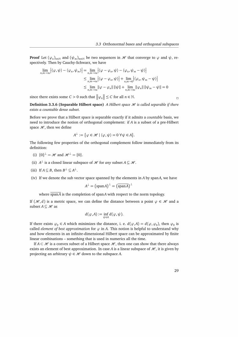
Proof Let (ϕn)n∈N and (ψm)m∈N be two sequences in H that converge to ϕ and ψ, re-spectively. Then by Cauchy-Schwarz, we have
limn,m→∞
⟨ϕ,ψ⟩ − ⟨ϕn,ψm⟩
= limn,m→∞
⟨ϕ−ϕn,ψ⟩ − ⟨ϕn,ψm −ψ⟩
≤ limn,m→∞
⟨ϕ−ϕn,ψ⟩
+ limn,m→0
⟨ϕn,ψm −ψ⟩
≤ limn,m→∞
‖ϕ−ϕn‖‖ψ‖+ limn,m→∞
‖ϕn‖‖ψm −ψ‖= 0
since there exists some C > 0 such that
ϕn
≤ C for all n ∈ N.
Definition 3.3.6 (Separable Hilbert space) A Hilbert spaceH is called separable if thereexists a countable dense subset.
Before we prove that a Hilbert space is separable exactly if it admits a countable basis, weneed to introduce the notion of orthogonal complement: if A is a subset of a pre-HilbertspaceH , then we define
A⊥ :=
ϕ ∈H | ⟨ϕ,ψ⟩= 0 ∀ψ ∈ A
.
The following few properties of the orthogonal complement follow immediately from itsdefinition:
(i) 0⊥ =H andH ⊥ = 0.
(ii) A⊥ is a closed linear subspace ofH for any subset A⊆H .
(iii) If A⊆ B, then B⊥ ⊆ A⊥.
(iv) If we denote the sub vector space spanned by the elements in A by span A, we have
A⊥ =
span A⊥ =
span A⊥
where span A is the completion of span A with respect to the norm topology.
If (H , d) is a metric space, we can define the distance between a point ϕ ∈ H and asubset A⊆H as
d(ϕ, A) := infψ∈A
d(ϕ,ψ).
If there exists ϕ0 ∈ A which minimizes the distance, i. e. d(ϕ, A) = d(ϕ,ϕ0), then ϕ0 iscalled element of best approximation for ϕ in A. This notion is helpful to understand whyand how elements in an infinite-dimensional Hilbert space can be approximated by finitelinear combinations – something that is used in numerics all the time.
If A⊂H is a convex subset of a Hilbert spaceH , then one can show that there alwaysexists an element of best approximation. In case A is a linear subspace ofH , it is given byprojecting an arbitrary ψ ∈H down to the subspace A.
29
3 Hilbert spaces
Theorem 3.3.7 Let A be a closed convex subset of a Hilbert space H . Then there exists foreach ϕ ∈H exactly one ϕ0 ∈ A such that
d(ϕ, A) = d(ϕ,ϕ0).
Proof We choose a sequence (ψn)n∈N in A with d(ϕ,ψn) =
ϕ−ψn
→ d(x , A). Thissequence is also a Cauchy sequence: we add and subtract ϕ to get
ψn −ψm
2=
(ψn −ϕ) + (ϕ−ψm)
2.
If H were a normed space, we could have to use the triangle inequality to estimate theright-hand side from above. However,H is a Hilbert space and by using the parallelogramidentity,1 we see that the right-hand side is actually equal to
ψn −ψm
2= 2
ψn −ϕ
2+ 2
ψm −ϕ
2 −
ψn +ψm − 2ϕ
2
= 2
ψn −ϕ
2+ 2
ψm −ϕ
2 − 4
12(ψn +ψm)−ϕ
2
≤ 2
ψn −ϕ
2+ 2
ψm −ϕ
2 − 4d(ϕ, A)n→∞−−→ 2d(ϕ, A) + 2d(ϕ, A)− 4d(ϕ, A) = 0.
By convexity, 12(ψn +ψm) is again an element of A. This is crucial once again for the
uniqueness argument. Letting n, m → ∞, we see that (ψn)n∈N is a Cauchy sequence inA which converges in A as it is a closed subset of H . Let us call the limit point ϕ0 :=limn→∞ψn. Then ϕ0 is an element of best approximation,
ϕ−ϕ0
= limn→∞
ϕ−ψn
= d(ϕ, A).
To show uniqueness, we assume that there exists another element of best approximationϕ′0 ∈ A. Define the sequence (ψn)n∈N by ψ2n := ϕ0 for even indices and ψ2n+1 := ϕ′0for odd indices. By assumption, we have
ϕ−ϕ0
= d(ϕ, A) =
ϕ−ϕ′0
and thus, byrepeating the steps above, we conclude (ψn)n∈N is a Cauchy sequence that converges tosome element. However, since the sequence is alternating, the two elements ϕ′0 = ϕ0 arein fact identical.
As we have seen, the condition that the set is convex and closed is crucial in the proof.Otherwise the minimizer may not be unique or even contained in the set.
Corrolary 3.3.8 Let E be a closed subvector space of the Hilbert space H . Then for anyϕ ∈H , there exists ϕ0 ∈ E such that d(ϕ, E) = d(ϕ,ϕ0).2009.11.04
1For all ϕ,ψ ∈H , the identity 2
ϕ
2+ 2
ψ
2=
ϕ+ψ
2+
ϕ−ψ
2holds.
30

3.3 Orthonormal bases and orthogonal subspaces
This is all very abstract. For the case of a closed subvector space E ⊆ H , we can expressthe element of best approximation in terms of the basis: not surprisingly, it is given by theprojection of ϕ onto E.
Theorem 3.3.9 Let E ⊆H be a closed subspace of a Hilbert space that is spanned by count-ably many orthonormal basis vectors ϕkk∈I . Then for any ϕ ∈ H , the element of bestapproximation ϕ0 ∈ E is given by
ϕ0 =∑
k∈I
⟨ϕk,ϕ⟩ϕk.
Proof It is easy to show that ϕ−ϕ0 is orthogonal to any ψ =∑
k∈I λkϕk ∈ E: we focuson the more difficult case when E is not finite dimensional: then, we have to approximateϕ0 and ψ by finite linear combinations and take limits. We call ϕ(n)0 :=
∑nk=1⟨ϕk,ϕ⟩ϕk
and ψ(m) :=∑m
l=1λl ϕl . With that, we have
ϕ−ϕ(n)0 ,ψ(m)
=D
ϕ−∑n
k=1⟨ϕk,ϕ⟩ϕk,∑m
l=1λl ϕl
E
=m∑
l=1
λl ⟨ϕ,ϕl⟩ −n∑
k=1
m∑
l=1
λl ⟨ϕk,ϕ⟩∗ ⟨ϕk,ϕl⟩
=m∑
l=1
λl ⟨ϕ,ϕl⟩
1−∑n
k=1 δkl
.
By continuity of the scalar product, Corollary 3.3.5, we can take the limit n, m→∞. Theterm in parentheses containing the sum is 0 exactly when l ∈ 1, . . . , m and 1 otherwise.Specifically, if n≥ m, the right-hand side vanishes identically. Hence, we have
ϕ−ϕ0,ψ
= limn,m→∞
ϕ−ϕ(n)0 ,ψ(m)
= 0,
in other words ϕ−ϕ0 ∈ E⊥. This, in turn, implies by the Pythagorean theorem that
ϕ−ψ
2=
ϕ−ϕ0
2+
ϕ0 −ψ
2 ≥
ϕ−ϕ0
2
and hence
ϕ−ϕ0
= d(ϕ, E). Put another way, ϕ0 is an element of best approximation.Let us now show uniqueness. Assume, there exists another element of best approximationϕ′0 =
∑
k∈I λ′kϕk. Then we know by repeating the previous calculation backwards that
ϕ−ϕ′0 ∈ E⊥ and the scalar product with respect to any of the basis vectors ϕk which spanE has to vanish,
0=
ϕk,ϕ−ϕ′0
= ⟨ϕk,ϕ⟩ −∑
l∈I
λ′l ⟨ϕk,ϕl⟩= ⟨ϕk,ϕ⟩ −∑
l∈I
λ′l δkl
= ⟨ϕk,ϕ⟩ −λ′k.
31

3 Hilbert spaces
This means the coefficients with respect to the basis ϕkk∈I all agree with those of ϕ0.Hence, the element of approximation is unique, ϕ0 = ϕ′0, and given by the projection ofϕ onto E.
Theorem 3.3.10 Let E be a closed linear subspace of a Hilbert spaceH . Then
(i) H = E ⊕ E⊥, i. e. every vector ϕ ∈ H can be uniquely decomposed as ϕ = ψ+ψ⊥
with ψ ∈ E, ψ⊥ ∈ E⊥.
(ii) E⊥⊥ = E.
Proof (i) By Theorem 3.3.7, for each ϕ ∈ H , there exists ϕ0 ∈ E such that d(ϕ, E) =d(ϕ,ϕ0). From the proof of the previous theorem, we see that ϕ⊥0 := ϕ−ϕ0 ∈ E⊥.Hence, ϕ = ϕ0 + ϕ⊥0 is a decomposition of ϕ. To show that it is unique, assumeϕ′0+ϕ
′0⊥ = ϕ = ϕ0+ϕ⊥0 is another decomposition. Then by subtracting, we are led
to conclude that
E 3 ϕ′0 −ϕ0 = ϕ⊥0 −ϕ
′0⊥ ∈ E⊥
holds. On the other hand, E ∩ E⊥ = 0 and thus ϕ0 = ϕ′0 and ϕ⊥0 = ϕ′0⊥, the
decomposition is unique.
(ii) It is easy to see that E ⊆ E⊥⊥. Let ϕ ∈ E⊥⊥. By the same arguments as above, wecan decompose ϕ ∈ E⊥⊥ ⊆H into
ϕ = ϕ0 + ϕ⊥0
with ϕ0 ∈ E ⊆ E⊥⊥ and ϕ⊥0 ∈ E⊥. Hence, ϕ − ϕ0 ∈ E⊥⊥ ∩ E⊥ = (E⊥)⊥ ∩ E⊥ = 0and thus ϕ = ϕ0 ∈ E.
Now we are in a position to prove the following important Proposition:
Proposition 3.3.11 A Hilbert space H is separable if and only if there exists a countableorthonormal basis.
Proof ⇐: The set generated by the orthonormal basis ϕ j j∈I , I countable, and coeffi-cients z = q+ ip, q, p ∈Q, is dense inH ,
n
∑nj=1z jϕ j ∈H
N 3 n≤ |I | , ϕ j ∈ ϕkk∈N, z j = q j + ip j , q j , p j ∈Qo
.
⇒: Assume there exists a countable dense subset D, i. e. D = H . If H is finite dimen-sional, the induction terminates after finitely many steps and the proof is simpler. Hence,
32

3.4 Subspaces (⊕) and product spaces (⊗)
we will assume H to be infinite dimensional. Pick a vector ϕ1 ∈ D \ 0 and normalizeit. The normalized vector is then called ϕ1. Note that ϕ1 need not be in D. By Theo-rem 3.3.10, we can split any ψ ∈ D into ψ1 and ψ⊥1 such that ψ1 ∈ span ϕ1 := E1,ψ⊥1 ∈ span ϕ1⊥ := E⊥1 and
ψ=ψ1 +ψ⊥1 .
pick a second ϕ2 ∈ D \ E1 (which is non-empty). Now we apply Theorem 3.3.9 (whichis in essence Gram-Schmidt orthonormalization) to ϕ2, i. e. we pick the part which isorthogonal to ϕ1,
ϕ′2 := ϕ2 − ⟨ϕ1, ϕ2⟩ϕ2
and normalize to ϕ2,
ϕ2 :=ϕ′2‖ϕ′2‖
.
This defines E2 := span ϕ1,ϕ2 andH = E2 ⊕ E⊥2 .Now we proceed by induction: assume we are given En = span ϕ1, . . . ,ϕn. Take
ϕn+1 ∈ D \ En and apply Gram-Schmidt once again to yield ϕn+1 which is the obtainedfrom normalizing the vector
ϕ′n+1 := ϕn+1 −n∑
k=1
⟨ϕk, ϕn+1⟩ϕk.
This induction yields an orthonormal sequence ϕnn∈N which is by definition an orthonor-mal basis of E∞ := span ϕnn∈N a closed subspace of H . If E∞ ( H , we can split theHilbert space into H = E∞ ⊕ E⊥∞. Then either D ∩ (H \ E∞) = ; – in which case D can-not be dense in H – or D ∩ (H \ E∞) 6= ;. But then we have terminated the inductionprematurely.
3.4 Subspaces (⊕) and product spaces (⊗)
There are several ways to split Hilbert spaces: in direct sums and direct products. Withthe same techniques, we can construct new ones from existing Hilbert spaces. In The-orem 3.3.10, we have shown that if E is a closed subspace, then H decomposes into adirect sum
H = E ⊕ E⊥.
That means any vector ϕ = ψ+ψ⊥ ∈ H can be uniquely decomposed into ψ ∈ E andψ⊥ ∈ E⊥. We now define the direct sum of two Hilbert spaces:
33

3 Hilbert spaces
Definition 3.4.1 (Direct sum ⊕) Let H1 and H2 be Hilbert spaces with scalar products⟨·, ·⟩1 and ⟨·, ·⟩2. Then we defineH1⊕H2 as the carteisan productH1×H2 of vector spacesendowed with the structure of a vector space in the following way: for any ϕ = (ϕ1,ϕ2),ψ=(ψ1,ψ2) ∈H1 ×H2 and α ∈ C, we define
(i) addition component-wise, ϕ+ψ= (ϕ1,ϕ2) + (ψ1,ψ2) := (ϕ1 +ψ1,ϕ2 +ψ2),
(ii) scalar multiplication component-wise, αϕ = α(ϕ1,ϕ2) := (αϕ1,αϕ2),
(iii) and the scalar product onH1 ⊕H2 is the sum of the two scalar products,
⟨ϕ,ψ⟩ := ⟨ϕ1,ψ1⟩1 + ⟨ϕ2,ψ2⟩2.
Proposition 3.4.2 The direct sumH1 ⊕H2 of two Hilbert spaces is a Hilbert space.
Proof One immediately checks that H1 ⊕H2 is a vector space. Completeness also fol-lows from the completeness of the components: let ϕ(n)n∈N be a Cauchy sequence withrespect to the norm induced by ⟨·, ·⟩. Writing out the definition, it is clear that this alsomeans each component ϕ(n)j n∈N, j = 1, 2, is a Cauchy sequence in H j which converges
to some ϕ j ∈H j . Hence, ϕ(n) −→ (ϕ1,ϕ2) as n→∞.
The other way to construct new Hibert spaces is taking tensor products: if ϕ1 ∈ H1 and2009.11.10ϕ2 ∈H2 are two vectors from two vector spaces, we can characterize ϕ1 ⊗ϕ2, the tensorproduct of ϕ1 and ϕ2, by the following defining properties: for any ϕ1,ψ1 ∈ H1 andϕ2,ψ2 ∈H2
ϕ1 ⊗ (ϕ2 +ψ2) = ϕ1 ⊗ϕ2 +ϕ1 ⊗ψ2
(ϕ1 +ψ1)⊗ϕ2 = ϕ1 ⊗ϕ2 +ψ1 ⊗ϕ2
holds. Scalars can be pushed back and forth between factors,
α(ϕ1 ⊗ϕ2) = (αϕ1)⊗ϕ2 = ϕ1 ⊗ (αϕ2).
The formal definition is a lot more complicated: one has to construct a big space wherevectors such as (αϕ1)⊗ ϕ2 and ϕ1 ⊗ (αϕ2) are distinct and then use equivalence rela-tions to implement the above characteristics. The constructed space is defined only up toisomorphism.
Definition 3.4.3 (Tensor product ⊗) Let H1 and H2 be two Hilbert spaces with scalarproducts ⟨·, ·⟩1 and ⟨·, ·⟩2. Then the tensor product H1 ⊗H2 is defined as the completion ofthe algebraic tensor product
H1 H2 :=n
∑nk=1λkϕ1 k ⊗ϕ2 k
n ∈ N, ϕ1 k ∈H1, ϕ2 k ∈H2, λk ∈ C∀1≤ k ≤ no
34

3.5 Linear functionals, dual space and weak convergence
with respect to the norm induced by the scalar product
⟨ϕ1 ⊗ϕ2,ψ1 ⊗ψ2⟩ := ⟨ϕ1,ψ1⟩1 ⟨ϕ2,ψ2⟩2, ∀ϕ1,ψ1 ∈H1, ϕ2,ψ2 ∈H2.
If ϕ1 kk∈I1and ϕ2 j j∈I2
are orthonormal bases of two separable Hilbert spacesH1 andH2, respectively, then
ϕ1 k ⊗ϕ2 j
k∈I1, j∈I2
is an orthonormal basis inH1 ⊗H2, i. e. every vector Ψ ∈H1 ⊗H2 can be written as∑
k∈I1j∈I2
ϕ1 k ⊗ϕ2 j ,Ψ
ϕ1 k ⊗ϕ2 j .
Example (i) A non-relativistic spin-1/2 particle lives in the Hilbert space L2(Rd ,C2).An easy, but very helpful exercise is to show the following equivalence (which cor-respond to different physical points of views):
L2(Rd ,C2)∼= L2(Rd)⊕ L2(Rd)∼= L2(Rd)⊗C2
Depending on the physical situation, these identification may be very helpful in solv-ing a problem.
(ii) Consider L2(Rd) ⊗ L2(Rd). This is the Hilbert space of two particles. If they areidentical, we have to restrict ourselves to the symmetric and antisymmetric subspace,depending on whether the particle in question is a boson or a fermion. Keep in mindthat in general, elements Ψ ∈ L2(Rd)⊗ L2(Rd) cannot be written as the product oftwo wave functions ϕ1,ϕ2 ∈ L2(Rd),
Ψ 6= ϕ1 ⊗ϕ2.
We will show in an exercise that L2(Rd)⊗ L2(Rd)∼= L2(Rd ×Rd).
3.5 Linear functionals, dual space and weak convergence
A very important notion is that of a functional. We have already gotten to know the freeenergy functional
Efree :D(Efree)⊂ L2(Rd)−→ [0,+∞)⊂ C,
ϕ 7→ Efree(ϕ) =1
2m
d∑
l=1
(−iħh∂x lϕ), (−iħh∂x l
ϕ)
.
This functional, however, is not linear, and it is not defined for all ϕ ∈ L2(Rd). Let usrestrict ourselves to a smaller class of functionals:
35
3 Hilbert spaces
Definition 3.5.1 (Bounded linear functional) Let X be a normed space. Then a map
L :X −→ C
is a bounded linear functional if and only if
(i) there exists C > 0 such that |L(x)| ≤ C ‖x‖ and
(ii) L(x +µy) = L(x) +µL(y)
hold for all x , y ∈ X and µ ∈ C.
A very basic fact is that boundedness of a linear functional is equivalent to its continuity.
Theorem 3.5.2 Let L : X −→ C be a linear functional on the normed space X . Then thefollowing statements are equivalent:
(i) L is continuous at x0 ∈ X .
(ii) L is continuous.
(iii) L is bounded.
Proof (i)⇔ (ii): This follows immediately from the linearity.
(ii)⇒ (iii): Assume L to be continuous. Then it is continuous at 0 and for ε = 1, we canpick δ > 0 such that
|L(x)| ≤ ε = 1
for all x ∈ X with ‖x‖ ≤ δ. By linearity, this implies for any y ∈ X \ 0 that
L δ
‖y‖ y
= δ
‖y‖
L(y)
≤ 1.
Hence, L is bounded with bound 1/δ,
L(y)
≤ 1δ
y
.
(iii)⇒ (ii): Conversely, if L is bounded by C > 0,
L(x)− L(y)
≤ C
x − y
,
holds for all x , y ∈ X . This means, L is continuous: for ε > 0 pick δ = ε/C so that
L(x)− L(y)
≤ C
x − y
≤ C ε
C= ε
holds for all x , y ∈ X such that
x − y
≤ ε/C.
36

3.5 Linear functionals, dual space and weak convergence
Definition 3.5.3 (Dual space) Let X be a normed space. The dual space X ∗ is the vectorspace of bounded linear functionals endowed with the norm
‖L‖∗ := supx∈X\0
|L(x)|‖x‖
= supx∈X‖x‖=1
|L(x)| .
Independently of whether X is complete, X ∗ is a Banach space.
Proposition 3.5.4 The dual space to a normed linear space X is a Banach space.
Proof Let (Ln)n∈N be a Cauchy sequence in X ∗, i. e. a sequence for which
Lk − L j
∗k, j→∞−−−→ 0.
We have to show that (Ln)n∈N converges to some L ∈ X ∗. For any ε > 0, there existsN(ε) ∈ N such that
Lk − L j
∗ < ε
for all k, j ≥ N(ε). This also implies that for any x ∈ X ,
Ln(x)
n∈N converges as well,
Lk(x)− L j(x)
≤
Lk − L j
∗ ‖x‖< ε ‖x‖ .
The field of complex numbers is complete and
Ln(x)
n∈N converges to some L(x) ∈ C.We now define
L(x) := limn→∞
Ln(x)
for any x ∈ X . Clearly, L inherits the linearity of the (Ln)n∈N. The map L is also bounded:for any ε > 0, there exists N(ε) ∈ N such that
L j − Ln
∗ < ε for all j, n≥ N(ε). Then
(L− Ln)(x)
= limj→∞
(L j − Ln)(x)
≤ limj //∞
L j − Ln
∗
x
< ε ‖x‖
holds for all n ≥ N(ε). Since we can write L as L = Ln + (L − Ln), we can estimate thenorm of the linear map L by ‖L‖∗ ≤ ‖Ln‖∗ + ε < ∞. This means L is a bounded linearfunctional on X .
In case of Hilbert spaces, the dualH ∗ can be canonically identified withH itself:
Theorem 3.5.5 (Riesz’ Lemma) LetH be a Hilbert space. Then for all L ∈H ∗ there existψL ∈H such that
L(ϕ) = ⟨ψL ,ϕ⟩.
In particular, we have ‖L‖∗ = ‖ψL‖.
37

3 Hilbert spaces
Proof Let ker L :=
ϕ ∈H | L(ϕ) = 0
be the kernel of the functional L and as such is aclosed linear subspace ofH . If ker L =H , then 0 ∈H is the associated vector,
L(ϕ) = 0= ⟨0,ϕ⟩.
So assume ker L (H is a proper subspace. Then we can splitH = ker L ⊕ (ker L)⊥. Pickϕ0 ∈ (ker L)⊥, i. e. L(ϕ0) 6= 0. Then define
ψL :=L(ϕ0)∗
‖ϕ0‖2 ϕ0.
We will show that L(ϕ) = ⟨ψL ,ϕ⟩. If ϕ ∈ ker L, then L(ϕ) = 0 = ⟨ψL ,ϕ⟩. One easilyshows that for ϕ = αϕ0, α ∈ C,
L(ϕ) = L(αϕ0) = α L(ϕ0)
= ⟨ψL ,ϕ⟩=D
L(ϕ0)∗
‖ϕ0‖2 ϕ0,αϕ0
E
= α L(ϕ0)⟨ϕ0,ϕ0⟩‖ϕ0‖2 = α L(ϕ0).
Every ϕ ∈H can be written as
ϕ =
ϕ−L(ϕ)L(ϕ0)
ϕ0
+L(ϕ)L(ϕ0)
ϕ0.
Then the first term is in the kernel of L while the second one is in the orthogonal comple-ment of ker L. Hence, L(ϕ) = ⟨ψL ,ϕ⟩ for all ϕ ∈ H . If there exists a second ψ′L ∈ H ,then for any ϕ ∈H
0= L(ϕ)− L(ϕ) = ⟨ψL ,ϕ⟩ − ⟨ψ′L ,ϕ⟩= ⟨ψL −ψ′L ,ϕ⟩.
This implies ψ′L =ψL and thus the element ψL is unique.To show ‖L‖∗ = ‖ψL‖, assume L 6= 0. Then, we have
‖L‖∗ = sup‖ϕ‖=1
L(ϕ)
≥
L ψL
‖ψL‖
=
ψL , ψL
‖ψL‖
= ‖ψL‖.
On the other hand, the Cauchy-Schwarz inequality yields
‖L‖∗ = sup‖ϕ‖=1
L(ϕ)
= sup‖ϕ‖=1
⟨ψL ,ϕ⟩
≤ sup‖ϕ‖=1
‖ψL‖‖ϕ‖= ‖ψL‖.
Putting these two together, we conclude ‖L‖∗ = ‖ψL‖.
38
3.5 Linear functionals, dual space and weak convergence
2009.11.11
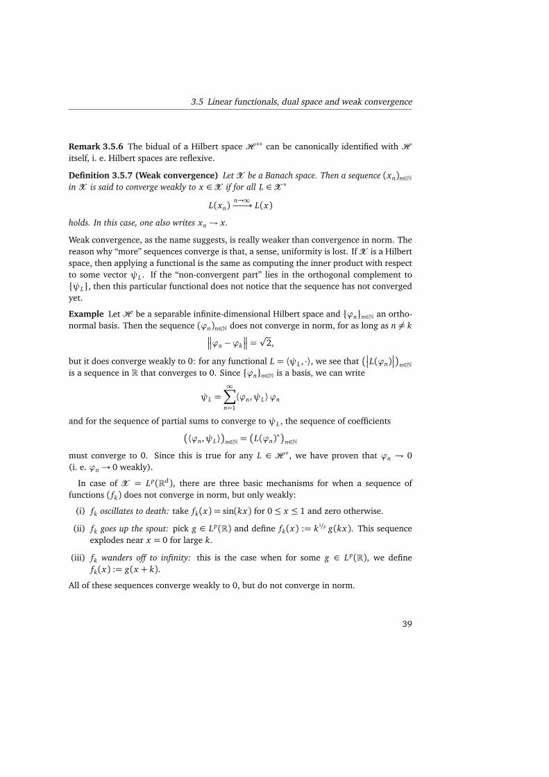
Remark 3.5.6 The bidual of a Hilbert space H ∗∗ can be canonically identified with Hitself, i. e. Hilbert spaces are reflexive.
Definition 3.5.7 (Weak convergence) Let X be a Banach space. Then a sequence (xn)n∈Nin X is said to converge weakly to x ∈ X if for all L ∈ X ∗
L(xn)n→∞−−→ L(x)
holds. In this case, one also writes xn * x.
Weak convergence, as the name suggests, is really weaker than convergence in norm. Thereason why “more” sequences converge is that, a sense, uniformity is lost. IfX is a Hilbertspace, then applying a functional is the same as computing the inner product with respectto some vector ψL . If the “non-convergent part” lies in the orthogonal complement toψL, then this particular functional does not notice that the sequence has not convergedyet.
Example LetH be a separable infinite-dimensional Hilbert space and ϕnn∈N an ortho-normal basis. Then the sequence (ϕn)n∈N does not converge in norm, for as long as n 6= k
ϕn −ϕk
=p
2,
but it does converge weakly to 0: for any functional L = ⟨ψL , ·⟩, we see that
L(ϕn)
n∈Nis a sequence in R that converges to 0. Since ϕnn∈N is a basis, we can write
ψL =∞∑
n=1
⟨ϕn,ψL⟩ϕn
and for the sequence of partial sums to converge to ψL , the sequence of coefficients
⟨ϕn,ψL⟩
n∈N =
L(ϕn)∗
n∈N
must converge to 0. Since this is true for any L ∈ H ∗, we have proven that ϕn * 0(i. e. ϕn→ 0 weakly).
In case of X = Lp(Rd), there are three basic mechanisms for when a sequence offunctions ( fk) does not converge in norm, but only weakly:
(i) fk oscillates to death: take fk(x) = sin(kx) for 0≤ x ≤ 1 and zero otherwise.
(ii) fk goes up the spout: pick g ∈ Lp(R) and define fk(x) := k1/p g(kx). This sequenceexplodes near x = 0 for large k.
(iii) fk wanders off to infinity: this is the case when for some g ∈ Lp(R), we definefk(x) := g(x + k).
All of these sequences converge weakly to 0, but do not converge in norm.
39
3 Hilbert spaces
3.6 Important facts on Lp(Rd)
For future reference, we collect a few facts on Lp(Rd) spaces. In particular, we will makeuse of dominated convergence frequently. We will give them without proof, they can befound in standard text books on analysis, see e. g. [LL01].
Definition 3.6.1 (Lp(Rd)) Let 1≤ p <∞. Then we define
L p(Rd) :=n
f : Rd −→ C
f measurable,
∫
Rd
dx
f (x)
p<∞
o
as the vector space of functions whose pth power is integrable. Then Lp(Rd) is the vectorspace
Lp(Rd) :=L p(Rd)/∼
consisting of equivalence classes of functions that agree almost everywhere. With the p norm
f
p :=∫
Rd
dx
f (x)
p1/p
it forms a normed space.
In case p =∞, we have to modify the definition a little bit.
Definition 3.6.2 (L∞(Rd)) We define
L∞(Rd) :=n
f : Rd −→ C
f measurable, ∃0< K <∞ :
f (x)
≤ K almost everywhereo
to be the space of functions that are bounded almost everywhere and
f
∞ := ess supx∈Rd
f (x)
:= inf
K ≥ 0
f (x)
≤ K for almost all x ∈ Rd.
Then the space L∞(Rd) := L∞(Rd)/ ∼ is defined as the vector space of equivalence classeswhere two functions are identified if they agree almost everywhere.
Theorem 3.6.3 (Riesz-Fischer) For any 1 ≤ p ≤ ∞, Lp(Rd) is complete with respect tothe ‖·‖p norm and thus a Banach space. If p = 2, L2(Rd) is also a Hilbert space with scalarproduct
f , g
=
∫
Rd
dx f (x)∗ g(x).
40

3.6 Important facts on Lp(Rd)
Theorem 3.6.4 For any 1≤ p ∞, the Banach space Lp(Rd) is separable.
Proof We refer to [LL01, Lemma 2.17] for an explicit construction. The idea is to approx-imate arbitrary functions by functions which are constant on cubes and take only valuesin the rational complex numbers.
Theorem 3.6.5 (Monotone Convergence) Let ( fk)k∈N be a sequence of non-decreasingfunctions in L1(Rd)with pointwise limit f defined almost everywhere. Define Ik :=
∫
Rd dx fk(x);then the sequence (Ik) is non-decreasing as well. If I := limk //∞ Ik < ∞, then I =∫
Rd dx f (x), i. e.
limk //∞
∫
Rd
dx fk(x) =
∫
Rd
dx limk //∞
fk(x) =
∫
Rd
dx f (x)
holds.
Theorem 3.6.6 (Dominated Convergence) Let ( fk)k∈N be a sequence of functions in L1(Rd)that converges almost everywhere pointwise to some f : Rd −→ C. If there exists a non-negative g ∈ L1(Rd) such that
fk(x)
≤ g(x) holds almost everywhere for all k ∈ N, then galso bounds
f
, i. e.
f (x)
≤ g(x) almost everywhere, and f ∈ L1(Rd). Furthermore, thelimit k //∞ and integration with respect to x commute and we have
limk //∞
∫
Rd
dx fk(x) =
∫
Rd
dx limk //∞
fk(x) =
∫
Rd
dx f (x).
41

3 Hilbert spaces
42

4 Linear operators
We will give a rough overview of operator theory. The most important section is that onselfadjointness which illuminates the connection between unitary evolution groups andselfadjoint operators.
4.1 Bounded operators
The simplest operators are bounded operators.
Definition 4.1.1 (Bounded operator) Let X and Y be normed spaces. A linear operatorT :X −→Y is called bounded if there exists M ≥ 0 with ‖T x‖Y ≤ M ‖x‖X .
Just as in the case of linear functionals, we have
Theorem 4.1.2 Let T : X −→ Y be a linear operator between two normed spaces X andY . Then the following statements are equivalent:
(i) T is continuous at x0 ∈ X .
(ii) T is continuous.
(iii) T is bounded.
Proof We leave it to the reader to modify the proof of Theorem 3.5.2.
We can introduce a norm on the operators which leads to a natural notion of convergence:
Definition 4.1.3 (Operator norm) Let T :X −→Y be a bounded linear operator betweennormed spaces. Then we define the operator norm of T as
‖T‖ := supx∈X‖x‖=1
‖T x‖Y .
The space of all bounded linear operators between X and Y is denoted byB(X ,Y ).
43

4 Linear operators
One can show that ‖T‖ coincides with
inf
M ≥ 0 | ‖T x‖Y ≤ M ‖x‖X ∀x ∈ X
= ‖T‖ .
The product of two bounded operators T ∈ B(Y ,Z ) and S ∈ B(X ,Y ) is again abounded operator and its norm can be estimated from above by
‖TS‖ ≤ ‖T‖‖S‖ .
If Y =X =Z , this implies that the product is jointly continuous with respect to the normtopology on X . For Hilbert spaces, the following useful theorem holds:
Theorem 4.1.4 (Hellinger-Toeplitz) Let A be a linear operator on a Hilbert spaceH withdense domain D(A) such that
ψ, Aϕ
=
Aψ,ϕ
holds for all ϕ,ψ ∈ D(A). Then D(A) =H if and only if A is bounded.
Proof ⇐: If A is bounded, then
Aϕ
≤ M
ϕ
for some M ≥ 0 and all ϕ ∈ H bydefinition of the norm. Hence, the domain of A is all ofH .
⇒: This direction relies on a rather deep result of functional analysis, the so-called OpenMapping Theorem and its corollary, the Closed Graph Theorem. The interested readermay look it up in Chapter III.5 of [RS81].
Let T, S be bounded linear operators between the normed spaces X and Y . If we define
(T + S)x := T x + Sx
as addition and
λ · T
x := λT x
as scalar multiplication, the set of bounded linear operators forms a vector space.
Proposition 4.1.5 The vector spaceB(X ,Y ) of bounded linear operators between normedspaces X and Y with operator norm forms a normed space. If Y is complete,B(X ,Y ) is aBanach space.
Proof The fact B(X ,Y ) is a normed vector space follows directly from the definition.To show that B(X ,Y ) is a Banach space whenever Y is, one has to modify the proof ofTheorem 3.5.4 to suit the current setting. This is left as an exercise.
Very often, it is easy to define an operator T on a “nice” dense subset D ⊆ X . Then thenext theorem tells us that if the operator is bounded, there is a unique bounded extensionof the operator to the whole space X . For instance, this allows us to instantly extend theFourier transform from Schwartz functions to L2(Rd) functions (see Proposition 5.1.9).
44
4.1 Bounded operators
Theorem 4.1.6 Let D ⊆ X be a dense subset of a normed space and Y be a Banach space.Furthermore, let T : D −→ Y be a bounded linear operator. Then there exists a uniquebounded linear extension T :X −→Y and ‖T‖= ‖T‖D .
Proof We construct T explicitly: let x ∈ X be arbitrary. Since D is dense in X , thereexists a sequence (xn)n∈N in D which converges to x . Then we set
T x := limn //∞
T xn.
First of all, T is linear. It is also well-defined: (T xn)n∈N is a Cauchy sequence in Y ,
T xn − T xk
Y ≤ ‖T‖D ‖xn − xk‖Xn,k //∞−−−−−→ 0,
where the norm of T is defined as
‖T‖D := supx∈D\0
‖T x‖Y‖x‖X
.
This Cauchy sequence in Y converges to some unique y ∈ Y as the target space is com-plete. Let (x ′n)n∈N be a second sequence in D that converges to x and assume the sequence(T x ′n)n∈N converges to some y ′ ∈ Y . We define a third sequence (zn)n∈N which alternatesbetween elements of the first sequence (xn)n∈N and the second sequence (x ′n)n∈N, i. e.
z2n−1 := xn
z2n := x ′n
for all n ∈ N. Then (zn)n∈N also converges to x and
Tzn
forms a Cauchy sequence thatconverges to, say, ζ ∈ Y . Subsequences of convergent sequences are also convergent andthey must converge to the same limit point. Hence, we conclude that
ζ= limn //∞
Tzn = limn //∞
Tz2n = limn //∞
T xn = y
= limn //∞
Tz2n−1 = limn //∞
T x ′n = y ′
holds and T x does not depend on the particular choice of sequence which approximatesx in D. It remains to show that ‖T‖= ‖T‖D : we can calculate the norm of T on the densesubset D and use that T |D = T to obtain
‖T‖= supx∈X‖x‖=1
‖T x‖= supx∈X\0
‖T x‖‖x‖
= supx∈D\0
‖T x‖‖x‖
= supx∈D\0
‖T x‖‖x‖
.
Hence, the norm of the extension T is equal to the norm of the original operator T .
45

4 Linear operators
The spectrum of an operator has been related to the set of possible outcomes of measure-ments (if the operator is selfadjoint).
Definition 4.1.7 (Spectrum) Let T ∈ B(X ) be a bounded linear operator on a Banachspace X . We define:
(i) The resolvent of T is the set ρ(T ) :=
λ ∈ C | T −λid is bijective
.
(ii) The spectrum σ(T ) := C \ρ(T ) is the complement of ρ(T ) in C.
One can show that for all λ ∈ ρ(T ), the map (T − λid)−1 is a bounded operator and thespectrum is a closed subset of C. One can show its σ(T ) is compact and contained in
λ ∈ C | |λ| ≤ ‖T‖
⊂ C.
4.2 Adjoint operator
IfX is a normed space, then we have definedX ∗, the space of bounded linear functionalson X . If T : X −→ Y is a bounded linear operator between two normed spaces, itnaturally defines the adjoint operator T ′ : Y ∗ −→X ∗ via
(T ′L)(x) := L(T x) (4.1)
for all x ∈ X and L ∈ Y ∗. In case of Hilbert spaces, one can associate the Hilbert spaceadjoint. We will almost exclusively work with the latter and thus drop “Hilbert space”most of the time.
Definition 4.2.1 (Hilbert space adjoint) Let H be a Hilbert space and A ∈ B(H ) be abounded linear operator on H . The antilinear isomorphism C : H −→ H ∗ taken fromTheorem 3.5.5 maps functionals on H onto the corresponding vectors, i. e. Cψ := ⟨ψ, ·⟩ =Lψ. Then the Hilbert space adjoint is defined as
A∗ := C−1A′C ,
or put differently
⟨A∗ϕ,ψ⟩ := ⟨ϕ, Aψ⟩
for all ϕ,ψ ∈H .2009.11.17
Proposition 4.2.2 Let A, B ∈B(H ) be two bounded linear operators on a Hilbert spaceHand α ∈ C. Then, we have:
(i) (A+ B)∗ = A∗ + B∗
46
4.2 Adjoint operator
(ii) (αA)∗ = α∗ A∗
(iii) (AB)∗ = B∗A∗
(iv) ‖A∗‖= ‖A‖
(v) A∗∗ = A
(vi) ‖A∗A‖= ‖AA∗‖= ‖A‖2
(vii) ker A= (im A∗)⊥, ker A∗ = (im A)⊥
Proof Properties (i)-(iii) follow directly from the defintion.To show (iv), we note that ‖A‖ ≤ ‖A∗‖ follows from
Aϕ
=
D
Aϕ‖Aϕ‖ , Aϕ
E
∗= sup‖L‖∗=1
L(Aϕ)
= sup‖ψL‖=1
A∗ψL ,ϕ
≤
A∗
ϕ
where in the step marked with ∗, we have used that we can calculate the norm frompicking the functional associated to Aϕ
‖Aϕ‖ : for a functional with norm 1, ‖L‖∗ = 1, thenorm of L(Aϕ) cannot exceed that of Aϕ
L(Aϕ)
= |⟨ψL , Aϕ⟩| ≤ ‖ψL‖‖Aϕ‖= ‖Aϕ‖.
Here, ψL is the vector such that L = ⟨ψL , ·⟩ which exists by Theorem 3.5.5. This theoremalso ensures ‖L‖∗ = ‖ψL‖. On the other hand, from
A∗ψL
=
LA∗ψL
∗ = sup‖ϕ‖=1
A∗ψL ,ϕ
≤ sup‖ϕ‖=1
ψL
Aϕ
= ‖A‖‖L‖∗ = ‖A‖‖ψL‖
we conclude ‖A∗‖ ≤ ‖A‖. Hence, ‖A∗‖= ‖A‖.(v) is clear. For (vi), we remark
‖A‖2 = sup‖ϕ‖=1
Aϕ
2= sup‖ϕ‖=1
ϕ, A∗Aϕ
≤ sup‖ϕ‖=1
A∗Aϕ
=
A∗A
.
This means
‖A‖2 ≤
A∗A
≤ ‖A∗‖‖A‖= ‖A‖2 .
47

4 Linear operators
which combined with (iv),
‖A‖2 =
A∗
2 ≤
AA∗
≤ ‖A‖
A∗
= ‖A‖2
implies ‖A∗A‖= ‖A‖2 = ‖AA∗‖. (vii) is left as an exercise.
Definition 4.2.3 LetH be a Hilbert space and A∈B(H ). Then A is called
(i) normal if A∗A= AA∗.
(ii) selfadjoint (or hermitian) if A∗ = A.
(iii) unitary if A∗A= idH = AA∗.
(iv) an orthogonal projection if A2 = A and A∗ = A.
(v) positive if
ϕ, Aϕ
≥ 0 for all ϕ ∈H .
4.3 Unitary operators
Unitary operators U have the nice property that
Uϕ, Uψ
=
ϕ, U∗Uψ
=
ϕ,ψ
for all ϕ,ψ ∈ H . In case of quantum mechanics, we are interested in solutions to theSchrödinger equation
id
dtψ(t) = Hψ(t), ψ(t) =ψ0,
for a hamilton operator which satisfies H∗ = H. Assume that H is bounded (this is reallythe case for many simple quantum systems). Then the unitary group generated by H,
U(t) = e−i tH ,
can be written as a power series,
e−i tH =∞∑
n=0
1
n!(−i t)n Hn
where H0 := id by convention. The sequence of partial sums converges in the operatornorm to e−i tH ,
N∑
n=0
1
n!(−i t)n Hn N //∞−−−−−→ e−i tH ,
48
4.3 Unitary operators
since we can make the simple estimate
∞∑
n=0
1
n!(−i t)n Hnψ
≤∞∑
n=0
1
n!|t|n
Hnψ
≤∞∑
n=0
1
n!|t|n ‖H‖n
ψ
= e|t|‖H‖
ψ
<∞.
This shows that the power series of the exponential converges in the operator norm inde-pendently of the choice of ψ to a bounded operator. Given a unitary evolution group, itis suggestive to obtain the hamiltonian which generates it by deriving U(t)ψ with respectto time. This is indeed the correct idea. The left-hand side of the Schrödinger equation(modulo a factor of i) can be expressed as a limit
d
dtψ(t) = lim
δ // 0
1δ
ψ(t +δ)−ψ(t)
.
This limit really exists, but before we compute it, we note that since
ψ(t +δ)−ψ(t) = e−i(t+δ)Hψ0 − e−i tHψ0 = e−i tHe−iδH − 1
ψ0,
it suffices to consider differentiability at t = 0: taking limits in norm ofH , we get
d
dtψ(0) = lim
δ // 0
1δ
ψ(δ)−ψ0
= limδ // 0
1
δ
∞∑
n=0
(−i)n
n!δnHnψ0 −ψ0
!
= limδ // 0
∞∑
n=1
(−i)n
n!δn−1Hnψ0 =−iHψ0.
Hence, we have established that e−i tHψ0 solves the Schrödinger condition with ψ(0) =ψ0,
id
dtψ(t) = Hψ(t).
However, this procedure does not work if H is unbounded (i. e. the generic case)! Beforewe proceed, we need to introduce several different notions of convergence of sequencesof operators which are necessary to define derivatives of U(t).
Definition 4.3.1 (Convergence of operators) Let An ∈ B(H ) be a sequence of boundedoperators. We say that the sequence converges to A∈B(H )
(i) uniformly/in norm if limn //∞
An − A
= 0.
(ii) strongly if limn //∞
Anψ− Aψ
= 0 for all ψ ∈H .
49
4 Linear operators
(iii) weakly if limn //∞
ϕ, Anψ− Aψ
= 0 for all ϕ,ψ ∈H .
Convergence of a sequence of operators in norm implies strong and weak convergence,but not the other way around. In the tutorials, we will also show explicitly that weakconvergence does not necessarily imply strong convergence.
Example With the arguments above, we have shown that if H = H∗ is selfadjoint andbounded, then t 7→ e−i tH is uniformly continuous.
If ‖H‖ = ∞ on the other hand, uniform continuity is too strong a requirement. If H =− 1
2∆x is the free Schrödinger operator on L2(Rd
x), then the Fourier transform F links theposition representation on L2(Rd
x) to the momentum representation on L2(Rdk). In this
representation, the free Schrödinger operator H simplifies to the multiplication operator
H = 12k2
acting on L2(Rdk). More elaborate mathematical arguments show that for any t ∈ R, the
norm of the difference between U(t) = e−i t 12
k2and U(0) = id
U(t)− id
= supk∈Rd
e−i t 12
k2− 1
= 2
is exactly 2 and U(t) cannot be uniformly continuous in t. However, if ψ ∈ L2(Rdk) is a
wave function, the estimate
U(t)ψ− ψ
2=
∫
Rdk
dk
e−i t 12
k2− 1
2 ψ(k)
2
≤ 22
∫
Rdk
dk
ψ(k)
2= 4
ψ
2
shows we can invoke the Theorem of Dominated Convergence to conclude U(t) is stronglycontinuous in t ∈ R.
Definition 4.3.2 (Strongly continuous one-parameter unitary group) A family of uni-tary operators U(t)t∈R on a Hilbert spaceH is called a strongly continuous one-parameterunitary group – or unitary group for short – if
(i) t 7→ U(t) is strongly continuous and
(ii) U(t)U(t ′) = U(t + t ′) as well as U(0) = idH
hold for all t, t ′ ∈ Rt .
50

4.3 Unitary operators
This is again a group representation of Rt just as in the case of the classical flow Φ. Theform of the Schrödinger equation,
id
dtψ(t) = Hψ(t),
also suggests that strong continuity/differentiability is the correct notion. Let us oncemore consider the free hamiltonian H =− 1
2∆x on L2(Rd
x). We have shown in the tutorialsthat its domain is
D(H) =
ϕ ∈ L2(Rdx) | −∆xϕ ∈ L2(Rd
x)
.
In Chapter 5, we will learn that D(H) is mapped by the Fourier transform onto
D(H) =
ψ ∈ L2(Rdk) | k
2ψ ∈ L2(Rdk)
.
Dominated Convergence can once more be used to make the following claims rigorous:for any ψ ∈ D(H), we have
limt // 0
it
U(t)− id)ψ− 12k2ψ
≤ limt // 0
it
U(t)− id)ψ
+
12k2ψ
. (4.2)
The second term is finite since ψ ∈ D(H) and we have to focus on the first term. On thelevel of functions,
limt // 0
it
e−i t 12
k2− 1
= id
dte−i t 1
2k2
t=0= 1
2k2
holds pointwise. Furthermore, by the mean value theorem, for any finite t ∈ R with|t| ≤ 1, for instance, then there exists 0≤ t0 ≤ t such that
1t
e−i t 12
k2− 1
= ∂t e−i t 1
2k2
t=t0=−i 1
2k2 e−i t0
12
k2.
This can be bounded uniformly in t by 12k2. Thus, also the first term can be bounded
by
12k2ψ
uniformly. By Dominated Convergence, we can interchange the limit t // 0and integration with respect to k on the left-hand side of equation (4.2). But then theintegrand is zero and thus the domain where the free evolution group is differentiablecoincides with the domain of the Fourier transformed hamiltonian, 2009.11.18
limt // 0
it
U(t)− id)ψ− 12k2ψ
= 0.
This suggests to use the following definition:
51

4 Linear operators
Definition 4.3.3 (Generator of a unitary group) A densely defined linear operator on aHilbert space H with domain D(H) ⊆ H is called generator of a unitary evolution groupU(t), t ∈ R, if
(i) the domain coincides with
áD(H) =n
ϕ ∈H
t 7→ U(t)ϕ differentiableo
= D(H)
(ii) and for all ψ ∈ D(H), the Schrödinger equation holds,
id
dtU(t)ψ= HU(t)ψ.
This is only one of the two implications: usually we are given a hamiltonian H and wewould like to know under which circumstances this operator generates a unitary evolutiongroup. We will answer this question conclusively in the next section with Stone’s Theorem.
Theorem 4.3.4 Let H be the generator of a strongly continuous evolution group U(t), t ∈ R.Then the following holds:
(i) D(H) is invariant under the action of U(t), i. e. U(t)D(H) = D(H) for all t ∈ R.
(ii) H commutes with U(t), i. e. [U(t), H]ψ := U(t)Hψ−H U(t)ψ= 0 for all t ∈ R andψ ∈ D(H).
(iii) H is symmetric, i. e.
Hϕ,ψ
=
ϕ, Hψ
holds for all ϕ,ψ ∈ D(H).
(iv) U(t) is uniquely determined by H.
(v) H is uniquely determined by U(t).
Proof (i) Let ψ ∈ D(H). To show that U(t)ψ is still in the domain, we have to showthat the norm of HU(t)ψ is finite. Since H is the generator of U(t), it is equal to
Hψ= id
dsU(s)ψ
s=0
= lims // 0
is
U(s)− id
ψ.
Let us start with s > 0 and omit the limit. Then
is
U(s)− id
U(t)ψ
=
U(t) is
U(s)− id
ψ
=
is
U(s)− id
ψ
<∞
holds for all s > 0. Taking the limit on left and right-hand side yields that we canestimate the norm of HU(t)ψ by the norm of Hψ – which is finite since ψ is in the
52
4.3 Unitary operators
domain. This means U(t)D(H) ⊆ D(H). To show the converse, we repeat the prooffor U(−t) = U(t)−1 = U(t)∗ to obtain
D(H) = U(−t)U(t)D(H)⊆ U(t)D(H).
Hence, U(t)D(H) = D(H).
(ii) This follows from an extension of the proof of (i): since the domain D(H) coincideswith the set of vectors on which U(t) is strongly differentiable and is left invariantby U(t), taking limits on left- and right-hand side of
is
U(s)− id
U(t)ψ− U(t) is
U(s)− id
ψ
= 0
leads to [H, U(t)]ψ= 0.
(iii) This follows from differentiating
U(t)ϕ, U(t)ψ
for arbitrary ϕ,ψ ∈ D(H) andusing
U(t), H
= 0 as well as the unitarity of U(t) for all t ∈ R.
(iv) Assume that both unitary evolution groups, U(t) and U(t), have H as their genera-tor. For any ψ ∈ D(H), we can calculate the time derivative of
(U(t)− U(t))ψ
2,
d
dt
(U(t)− U(t))ψ
2= 2
d
dt
ψ
2 −Re
U(t)ψ, U(t)ψ
=−2Re
−iHU(t)ψ, U(t)ψ
+
U(t)ψ,−iHU(t)ψ
= 0.
Since U(0) = id = U(0), this means U(t) and U(t) agree at least on D(H). Usingthe fact that there is only bounded extension of a bounded operator to all of H ,Theorem 4.1.6, we conclude they must be equal on all ofH .
(v) This follows from the definition of the generator and the density of the domain.
Now that we have collected a few facts on unitary evolution groups, one could think thatsymmetric operators generate evolution groups, but this is false! The standard exampleto showcase this fact is the group of translations on L2([0, 1]). Since we would like T (t)to conserve “mass” – or more accurately, probability, we define for ϕ ∈ L2([0,1]) and0≤ t < 1
T (t)ϕ
(x) :=
¨
ϕ(x − t) x − t ∈ [0, 1]ϕ(x − t + 1) x − t + 1 ∈ [0, 1]
.
53

4 Linear operators
For all other t ∈ R, we extend this operator periodically, i. e. we plug in the fractionalpart of t. Clearly,
T (t)ϕ, T (t)ψ
=
ϕ,ψ
holds for all ϕ,ψ ∈ L2([0,1]). Locally, theinfinitesimal generator is −i∂x as a simple calculation shows:
id
dt
T (t)ϕ
(x)
t=0
= id
dtϕ(x − t)
t=0
=−i∂xϕ(x)
However, T (t) does not respect the maximal domain of −i∂x ,
Dmax(−i∂x) =
ϕ ∈ L2([0, 1]) | − i∂xϕ ∈ L2([0,1])
.
Any element of the maximal domain has a continuous representative, but if ϕ(0) 6= ϕ(1),then for t > 0, T (t)ϕ will have a discontinuity at t. We will denote the operator −i∂x
on Dmax(−i∂x) with Pmax. Let us check whether Pmax is symmetric: for any ϕ,ψ ∈Dmax(−i∂x), we compute
ϕ,−i∂xψ
=
∫ 1
0
dx ϕ∗(x) (−i∂xψ)(x) =h
−iϕ∗(x)ψ(x)i1
0−∫ 1
0
dx (−i)∂xϕ∗(x)ψ(x)
= i
ϕ∗(0)ψ(0)−ϕ∗(1)ψ(1)
+
∫ 1
0
dx (−i∂xϕ)∗(x)ψ(x)
= i
ϕ∗(0)ψ(0)−ϕ∗(1)ψ(1)
+
−i∂xϕ,ψ
. (4.3)
In general, the boundary terms do not disappear and the maximal domain is “too large”for −i∂x to be symmetric. Thus it is not at all surprising, T (t) does not leave Dmax(−i∂x)invariant. Let us try another domain: one way to make the boundary terms disappear isto choose
Dmin(−i∂x) :=n
ϕ ∈ L2([0,1])
− i∂xϕ ∈ L2([0,1]), ϕ(0) = 0= ϕ(1)o
.
We denote −i∂x on this “minimal” domain with Pmin. In this case, the boundary terms inequation (4.3) vanish which tells us that Pmin is symmetric. Alas, the domain is still notinvariant under translations T (t), even though Pmin is symmetric. This is an example of asymmetric operator which does not generate a unitary group.
There is another thing we have missed so far: the translations allow for an additionalphase factor, i. e. for ϕ,ψ ∈ L2([0, 1]) and ϑ ∈ [0, 2π), we define for 0≤ t < 1
Tϑ(t)ϕ
(x) :=
¨
ϕ(x − t) x − t ∈ [0,1]eiϑϕ(x − t + 1) x − t + 1 ∈ [0, 1]
.
while for all other t, we plug in the fractional part of t. The additional phase factorcancels in the inner product,
Tϑ(t)ϕ, Tϑ(t)ψ
=
ϕ,ψ
still holds true for all ϕ,ψ ∈
54
4.4 Selfadjoint operators
L2([0, 1]). In general Tϑ(t) 6= Tϑ′(t) if ϑ 6= ϑ′ and the unitary groups are genuinelydifferent. Repeating the simple calculation from before, we see that the local generatorstill is −i∂x and it would seem we can generate a family of unitary evolutions from asingle generator. The confusion is resolved if we focus on invariant domains: choosingϑ ∈ [0,2π), we define Pϑ to be the operator −i∂x on the domain
Dϑ(−i∂x) :=n
ϕ ∈ L2([0,1])
− i∂xϕ ∈ L2([0,1]), ϕ(0) = e−iϑϕ(1)o
.
A quick look at equation (4.3) reassures us that Pϑ is symmetric and a quick calculationshows it is also invariant under the action of Tϑ(t). Hence, Pϑ is the generator of Tϑ, andthe definition of an unbounded operator is incomplete without spelling out its domain.
Example Another example where the domain is crucial in the properties is the waveequation on [0, L],
∂ 2t u(x , t)− ∂ 2
x u(x , t) = 0, u ∈ C 2([0, L]×Rt).
Here, u is the amplitude of the vibration, i. e. the lateral deflection. If we choose Dirichletboundary conditions at both ends, i. e. u(0) = 0 = u(L), we model a closed pipe, if wechoose Dirichlet boundary conditions on one end, u(0) = 0, and von Neumann boundaryconditions on the other, u′(L) = 0, we model a half-closed pipe. Choosing domains is aquestion of physics!
4.4 Selfadjoint operators
Although we do not have time to explore this very far, the crucial difference between Pmin
and Pϑ is that the former is only symmetric while the latter is also selfadjoint. We firstrecall the definition of the adjoint of a possibly unbounded operator:
Definition 4.4.1 (Adjoint operator) Let A be a densely defined linear operator on a Hilbertspace H with domain D(A). Let D(A∗) be the set of ϕ ∈ H for which there exists φ ∈ Hwith
Aψ,ϕ
=
ψ,φ
∀ψ ∈ D(A).
For each ϕ ∈ D(A∗), we define A∗ϕ := φ and A∗ is called the adjoint of A.
Remark 4.4.2 By Riesz Lemma, ϕ belongs to D(A∗) if and only if
Aψ,ϕ
≤ C
ψ
∀ψ ∈ D(A).
This is equivalent to saying ϕ ∈ D(A∗) if and only if ψ 7→ ⟨Aψ,ϕ⟩ is continuous on D(A).As a matter of fact, we could have used to latter to define the adjoint operator.
55

4 Linear operators
One word of caution: even if A is densely defined, A∗ need not be.
Example Let f ∈ L∞(R), but f 6∈ L2(R), and pick ψ0 ∈ L2(R). Define
D(T f ) :=n
ψ ∈ L2(R) |∫
Rdx
f (x)ψ(x)
<∞o
.
Then the adjoint of the operator
T fψ := ⟨ f ,ψ⟩ψ0, ψ ∈ D(T f ),
has domain D(T ∗f ) = 0. Let ψ ∈ D(T f ). Then for any ϕ ∈ D(T ∗f )
T fψ,ϕ
=
⟨ f ,ψ⟩ψ0,ϕ
=
ψ, f
ψ0,ϕ
=
ψ, ⟨ψ0,ϕ⟩ f
.
Hence T ∗f ϕ = ⟨ψ0,ϕ⟩ f . However f 6∈ L2(R) and thus ϕ = 0 is the only possible choicefor which T ∗f ϕ is well defined.
Symmetric operators, however, are special: since
Aϕ,ψ
=
ϕ, Aψ
holds by definitionfor all ϕ,ψ ∈ H , the domain of A∗ is contained in that of A, D(A∗) ⊇ D(A). In particular,D(A∗)⊆H is also dense. Thus, A∗ is an extension of A.
Definition 4.4.3 (Selfadjoint operator) Let H be a symmetric operator on a Hilbert spaceH with domain D(H). H is called selfadjoint, H∗ = H, if D(H∗) = D(H).
One word regarding notation: if we write A∗ = A, we do not just imply that the “operatorprescription” of A and A∗ is the same, but that the domains of both coincide.
Example In this sense, P∗min 6= Pmin.
The central theorem of this section is Stone’s Theorem:
Theorem 4.4.4 (Stone) To every strongly continuous one-parameter unitary group U on aHilbert space H , there exists a selfadjoint operator H = H∗ which generates U(t) = e−i tH .Conversely, every selfadjoint operator H generates the unitary evolution group U(t) = e−i tH .
A complete proof [RS81, Chapter VIII.3] is beyond our capabilities.2009.11.24
56
5 Schwartz functions and tempereddistributions
Schwartz functions are a space of test functions, i. e. a space of “very nicely behavedfunctions.” The dual of this space of test functions, the tempered distributions, allow usto extend common operations such as Fourier transforms and derivatives to objects whichmay not even be functions.
5.1 Schwartz functions
The motivation to define Schwartz functions on Rd comes from dealing with Fourier trans-forms: our class of test functions S (Rd) has three defining properties:
(i) S (Rd) forms a vector space.
(ii) Stability under derivation, ∂ αx S (Rd) ⊂ S (Rd): for all multiindices α ∈ Nd
0 andf ∈ S (Rd), we have ∂ αx f ∈ S (Rd).
(iii) Stability under Fourier transform, FS (Rd) ⊆ S (Rd): for all f ∈ S (Rd), the Fouriertransform
F±1 f : ξ 7→1
(2π)d/2
∫
Rd
dx e∓i x ·ξ f (x) ∈ S (Rd) (5.1)
is also a test function.
These relatively simple requirements have surprisingly rich implications:
(i) S (Rd)⊂ L1(Rd), i. e. any f ∈ S (Rd) and all of its derivatives are integrable.
(ii) F : S (Rd) −→ S (Rd) acts bijectively: if f ∈ S (Rd) ⊂ L1(Rd), then F f ∈ S (Rd) ⊂L1(Rd).
(iii) For all α ∈ Nd0 , we have F
(i∂x)α f
= xα F f ∈ S (Rd). This holds as all derivativesare integrable.
(iv) Hence, for all a,α ∈ Nd0 , we have xa∂ αx f ∈ S .
57

5 Schwartz functions and tempered distributions
(v) Translations of Schwartz functions are again Schwartz functions, f (·− x0) ∈ S (Rd);this follows from F f (· − x0) = e−iξ·x0 F f ∈ S (Rd) for all x0 ∈ Rd .
This leads to the following definition:
Definition 5.1.1 (Schwartz functions) The space of Schwartz functions
S (Rd) :=n
f ∈ C∞(Rd)
∀a,α ∈ Nd0 :
f
aα <∞o
is defined in terms of the family of seminorms1 indexed by a,α ∈ Nd0
f
aα := supx∈Rd
xa∂ αx f (x)
, f ∈ C∞(Rd).
The family of seminorms defines a so-called Fréchet topology: put in simple terms, to makesure that sequences in S (Rd) converge to rapidly decreasing smooth functions, we needto control all derivatives as well as the decay. This is also the reason why there is nonorm on S (Rd) which generates the same topology as the family of seminorms. However,
f
aα = 0 for all a,α ∈ Nd0 ensures f = 0, all seminorms put together can distinguish
points.
Example Two simple examples of Schwartz functions are
f (x) = e−ax2, a > 0,
and
g(x) =
¨
e−1
1−x2 +1 |x |< 10 |x | ≥ 1
.
The second one even has compact support.
The first major fact we will establish is completeness.
Theorem 5.1.2 The space of Schwartz functions endowed with
d( f , g) :=∞∑
n=0
2−n sup|a|+|α|=n
f − g
aα
1+
f − g
aα
is a complete metric space.
1A seminorm has all properties of a norm except that
f
= 0 does not necessarily imply f = 0.
58
5.1 Schwartz functions
Proof d is positive and symmetric. It also satisfies the triangle inequality as x 7→ x1+x
is
concave on R+0 and all of the seminorms satisfy the triangle inequality. Hence,
S (Rd), d
is a metric space.To show completeness, take a Cauchy sequence ( fn) with respect to d. By definition and
positivity, this means ( fn) is also a Cauchy sequence with respect to all of the seminorms‖·‖aα. Each of the
xa∂ αx fn
converge to some gaα as the space of bounded continuousfunctions BC (Rd) with sup norm is complete. It remains to show that gaα = xa∂ αx g00.Clearly, only taking derivatives is problematic: we will prove this for |α| = 1, the generalresult follows from a simple induction. Assume we are interested in the sequence (∂xk
fn),k ∈ 1, . . . , d. With αk := (0, . . . , 0, 1, 0, . . .) as the multiindex that has a 1 in the kth entryand ek := (0, . . . , 0, 1, 0, . . .) ∈ Rd as the kth canonical base vector, we know that
fn(x) = fn(x − xkek) +
∫ xk
0
ds ∂xkfn
x + (s− xk)ek
as well as
g00(x) = g00(x − xkek) +
∫ xk
0
ds ∂xkg00
x + (s− xk)ek
hold since fn// g00 and ∂xk
fn// g0αk
uniformly. Hence, g00 ∈ C 1(Rd) and the derivativeof g00 coincides with g0αk
, ∂xkg00 = g0αk
. We then proceed by induction to show g00 ∈C∞(Rd). This means d( fn, g00) // 0 as n //∞ and S (Rd) is complete.
The Lp norm of each element in S (Rd) can be dominated by two seminorms:
Lemma 5.1.3 Let f ∈ S (Rd). Then for each 1 ≤ p <∞, the Lp norm of f can be domi-nated by a finite number of seminorms,
f
Lp(Rd ) ≤ C1(d)
f
00 + C2(d) max|a|=2n(d)
f
a0 ,
where C1(d), C2(d) ∈ R+ and n(d) ∈ N0 only depend on the dimension of Rd . Hence,f ∈ Lp(Rd).
Proof We split the integral on Rd into an integral over the unit ball centered at the originand its complement: let Bn :=max|a|=2n
f
a0, then
f
Lp(Rd ) =∫
Rd
dx
f (x)
p1/p
≤∫
|x |≤1
dx
f (x)
p1/p
+∫
|x |>1
dx
f (x)
p1/p
≤
f
00
∫
|x |≤1
dx 11/p
+∫
|x |>1
dx
f (x)
p |x |2np
|x |2np
1/p
≤ Vol(B1(0))1/p
f
00 + Bn
∫
|x |>1
dx1
|x |2np
1/p
.
59

5 Schwartz functions and tempered distributions
If we choose n large enough, |x |−2np is integrable and can be computed explicitly, and weget
f
Lp(Rd ) ≤ C1(d)
f
00 + C2(d) max|a|=2n
f
a0 .
This concludes the proof.
Lemma 5.1.4 The smooth functions with compact support C∞c (Rd) are dense in S (Rd).
Proof Take any f ∈ S (Rd) and take
g(x) =
¨
e−1
1−x2 +1 |x | ≤ 10 |x |> 1
.
Then fn := g(·/n) f converges to f in S (Rd), i. e.
limn //∞
fn − f
aα = 0
holds for all a,α ∈ Nd0 .
Next, we will show that F : S (Rd) −→ S (Rd) is a continuous and bijective map fromS (Rd) onto itself.
Theorem 5.1.5 The Fourier transform F as defined by equation (5.1) maps S (Rd) contin-uously and bijectively onto itself. The inverse F−1 is continuous as well. Furthermore, for allf ∈ S (Rd) and a,α ∈ Nd
0 , we have
F
xa(+i∂x)α f
= (+i∂ξ)aξαF f . (5.2)
Proof We need to prove F
xa(+i∂x)α f
= (+i∂ξ)aξαF f first: since xα∂ ax f is integrable,
its Fourier transform exists and is continuous by Dominated Convergence. For any a,α ∈Nd
0 , we have
F
xa(+i∂x)α f
(ξ) =1
(2π)d/2
∫
Rd
dx e−i x ·ξ xa (+i∂x)α f (x)
=1
(2π)d/2
∫
Rd
dx (+i∂ξ)ae−i x ·ξ (+i∂x)
α f (x)
∗=
1
(2π)d/2(+i∂ξ)
a
∫
Rd
dx e−i x ·ξ (+i∂x)α f (x).
60
5.1 Schwartz functions
In the step marked with ∗, we have used Dominated Convergence to interchange integra-tion and differentiation. Now we integrate partially |α| times and use that the boundaryterms vanish,
F
xa(+i∂x)α f
(ξ) =1
(2π)d/2(+i∂ξ)
a
∫
Rd
dx (+i∂x)αe−i x ·ξ f (x)
=1
(2π)d/2(+i∂ξ)
a
∫
Rd
dx ξαe−i x ·ξ f (x)
=
(+i∂ξ)aξαF f
(ξ).
To show F is continuous, we need to estimate the seminorms of F f by those of f : for anya,α ∈ Nd
0 , it holds
F f
aα = supξ∈Rd
ξa∂ αξ F f
(ξ)
= supξ∈Rd
F
∂ ax xα f
(x)
≤1
(2π)d/2
∂ ax xα f
L1(Rd ).
In particular, this implies F f ∈ S (Rd). Since ∂ ax xα f ∈ S (Rd), we can apply Lemma 5.1.3
and estaimte the right-hand side by a finite number of seminorms of f . Hence, F iscontinuous: if fn is a Cauchy sequence in S (Rd) that converges to f , then F fn has toconverge to F f ∈ S (Rd).
To show that F is a bijection with continuous inverse, we note that it suffices to proveF−1F f = f for functions f in a dense subset, namely C∞c (R
d) (see Lemma 5.1.4). Pick fso that the support of is contained in a cube Wn with sides of length 2n. We can write fon Wn as a uniformly convergent Fourier series,
f (x) =∑
ξ∈ πnZd
f (ξ)ei x ·ξ,
with
f (ξ) =1
Vol(Wn)
∫
Wn
dx e−i x ·ξ f (x) =(2π)d/2
(2n)d1
(2π)d/2
∫
Rd
dx e−i x ·ξ f (x).
Hence, f can be expressed as
f (x) =∑
ξ∈ πnZd
1
(2π)d/2
πd
nd(F f )(ξ) ei x ·ξ
61

5 Schwartz functions and tempered distributions
which is a Riemann sum that converges to
f (x) =1
(2π)d/2
∫
Rd
dx ei x ·ξ (F f )(ξ) =
F−1F f
(x)
as F f ∈ S . This concludes the proof.
Hence, we have shown that S (Rd) has the defining properties that suggested its moti-vation in the first place. The Schwartz functions also have other nice properties whoseproofs are left as an exercise.2009.11.25
Proposition 5.1.6 The Schwartz functions have the following properties:
(i) With pointwise multiplication · : S (Rd) × S (Rd) −→ S (Rd), the space of S (Rd)forms a Fréchet algebra (i. e. the multiplication is continuous in both arguments).
(ii) For all a,α, the map f 7→ xa∂ αξ f is continuous on S (Rd).
(iii) For any x0 ∈ Rd , the map τx0: f 7→ f (· − x0) continuous on S (Rd).
(iv) For any f ∈ S , 1h
τhekf − f ) converges to ∂xk
f as h //0 where ek is the kth canonicalbase vector of Rd .
The next important fact will be mentioned without proof:
Theorem 5.1.7 S (Rd) is dense in Lp(Rd), 1≤ p <∞.
This means, we can approximate any Lp(Rd) function by a test function. We will use thisand the next theorem to extend the Fourier transform to L2(Rd).
Theorem 5.1.8 For all f , g ∈ S (Rd), we have∫
Rd
dx (F f )(x) g(x) =
∫
Rd
dx f (x) (Fg)(x).
This implies ⟨F f , g⟩= ⟨ f ,F−1 g⟩ and ⟨F f ,Fg⟩= ⟨ f , g⟩ where ⟨·, ·⟩ is the usual scalar producton L2(Rd).
Proof Using Fubini’s theorem, we conclude we can first integrate with respect to ξ insteadof x ,∫
Rd
dx (F f )(x) g(x) =
∫
Rd
dx1
(2π)d/2
∫
Rd
dξ e−i x ·ξ f (ξ) g(x)
=
∫
Rd
dξ f (ξ)1
(2π)d/2
∫
Rd
dx e−i x ·ξg(x) =
∫
Rd
dξ f (ξ) (Fg)(ξ).
62
5.1 Schwartz functions
To prove the second part, we remark that compared to the scalar product on L2(Rd), weare missing a complex conjugation of the first function. Furthermore, (F f )∗ = F−1 f ∗
holds. From this, it follows that ⟨F f , g⟩ = ⟨ f ,F−1 g⟩ and upon replacing g with Fg, that⟨F f ,Fg⟩= ⟨ f ,F−1Fg⟩= ⟨ f , g⟩.
This has a nice consequence: since S (Rd) ⊂ L2(Rd) is dense and the Fourier transformacts unitarily on S (Rd) with respect to the scalar product, i. e. the Fourier transform isbounded, Theorem 4.1.6 allows us to extend F : S (Rd) −→S (Rd) to a unitary operatorF : L2(Rd)−→ L2(Rd). Hence, we have just proven
Proposition 5.1.9 The Fourier transform F : S (Rd) −→S (Rd) extends to a unitary oper-ator F : L2(Rd)−→ L2(Rd).
Now we will apply this to the free Schrödinger operator H = − 12∆x . First of all, we
conclude from Theorem 5.1.7 that the domain of H,
S (Rd)⊂ D(H) =
ϕ ∈ L2(Rd) | −∆xϕ ∈ L2(Rd)
⊂ L2(Rd),
is dense. So let us pick initial conditions such that ψ0 ∈ S (Rd) ⊂ L2(Rd). Then we canFourier transform the free Schrödinger equation,
F
i∂tψ(t)
= i∂tFψ(t) = F
− 12∆xψ(t)
= F
− 12∆x
F−1Fψ(t).
If we compute the right-hand side at t = 0, by Theorem 5.1.5 this leads to
F
− 12∆xψ0
(ξ) = 12ξ2 (Fψ0)(ξ).
Denoting the Fourier transform of ψ by ψ, this means the free Schrödinger equation inthe momentum representation reads
id
dtψ(t) = 1
2ξ2ψ(t), ψ(0) = ψ0.
We have already proven in section 4.3 that the unitary time evolution generated by H =12ξ2 is e−i t 1
2ξ2
. Sandwiching the unitary time evolution in the momentum representationin between Fourier transforms (which are themselves unitary on L2(Rd)) yields the timeevolution in the position representation.
Proposition 5.1.10 Let ψ0 ∈ S (Rd) ⊂ L2(Rd). Then for t 6= 0 the global solution of thefree Schrödinger equation with initial condition ψ0 is given by
ψ(x , t) =1
(2πi t)d/2
∫
Rd
dy ei (x−y)2
2t ψ0(y) =:
∫
Rd
dy p(x , y, t)ψ0(y). (5.3)
This expression converges in the L2 norm to ψ0 as t // 0.
63
5 Schwartz functions and tempered distributions
Proof We denote the Fourier transform of e−i t 12ξ2
by
U(t) := F−1e−i t 12ξ2F.
If t = 0, then the bijectivity of the Fourier transform on S (Rd), Theorem 5.1.5, yieldsU(0) = idS .
So let t 6= 0. If ψ0 is a Schwartz function, so is e−i t 12ξ2ψ0. As the Fourier transform is
a unitary map on L2(Rd) (Theorem 5.1.9) and maps Schwartz functions onto Schwartzfunctions (Theorem 5.1.5), U(t) also maps Schwartz functions onto Schwartz functions.Plugging in the definition of the Fourier transform, for any ψ0 ∈ S (Rd) and t 6= 0 we canwrite out U(t)ψ0 as
F−1e−i t 12ξ2Fψ0
(x) =1
(2π)d
∫
Rd
dξ e+i x ·ξ e−i t 12ξ2
∫
Rd
dy e−i y·ξψ0(y)
=1
(2π)d/2
∫
Rd
dξ
∫
Rd
dy ei (x−y)2
2t
1
(2π)d/2e−i t
2(ξ−(x−y)/t)2
ψ0(y). (5.4)
We need to regularize the integral: if we write the right-hand side of the above as
r. h. s.= limε0
1
(2π)d/2
∫
Rd
dξ
∫
Rd
dy ei (x−y)2
2t
1
(2π)d/2e−(ε+i) t
2(ξ−(x−y)/t)2
ψ0(y)
= limε0
1
(2π)d/2
∫
Rd
dy ei (x−y)2
2t
1
(2π)d/2
∫
Rd
dξ e−(ε+i) t2(ξ−(x−y)/t)2
ψ0(y),
we can use Fubini to change the order of integration. The inner integral can be computedby interpreting it as an integral in the complex plane,
1
(2π)d/2
∫
Rd
dξ e−(ε+i) t2(ξ−(x−y)/t)2 =
1
(ε+ i)td/2
.
Plugged back into equation (5.4) and combined with the Theorem of Monotone Conver-gence, this yields equation (5.3).
Later on, we will need the convolution,
( f ∗ g)(x) :=
∫
Rd
dy f (x − y) g(y),
for the Moyal product the product which emulates the operator product on the level offunctions. The convolution is an abelian product on S (Rd), i. e. f ∗ g = g ∗ f is satisfiedfor all f , g ∈ S (Rd).
64

5.2 Tempered distributions
Proposition 5.1.11 S (Rd) ∗S (Rd)⊆ S (Rd)
Proof Let f , g ∈ S (Rd). As F( f ∗ g) = (2π)d/2F f Fg,
F( f ∗ g)
(ξ) =1
(2π)d/2
∫
Rd
dx e−i x ·ξ∫
Rd
dy f (x − y) g(y)
=1
(2π)d/2
∫
Rd
dx e−i(x−y)·ξ∫
Rd
dy f (x − y) e−i y·ξ g(y)
= (2π)d/2(F f )(ξ) (Fg)(ξ),
we see that f ∗ g = (2π)d/2F−1F f Fg
∈ S (Rd).
5.2 Tempered distributions
Tempered distributions are linear functionals on S (Rd).
Definition 5.2.1 (Tempered distributions) The tempered distributionsS ′(Rd) are the con-tinuous linear functions on the Schwartz functions S (Rd). If L ∈ S ′(Rd) is a linear func-tional, we will often write
L, f
:= L( f ) ∀ f ∈ S (Rd).
Example (i) The δ distribution defined via
δ( f ) := f (0)
is a linear continuous functional on S (Rd). (See exercise sheet 6.)
(ii) Let g ∈ Lp(Rd), 1≤ p <∞, then for f ∈ S (Rd), we define
Lg( f ) =
∫
Rd
dx g(x) f (x) =:
g, f
. (5.5)
As f ∈ S (Rd)⊂ Lq(Rd), 1p+ 1
q= 1, by Hölder’s inequality, we have
g, f
≤
g
p
f
q .
Since
f
q can be bounded by a finite linear combination of Fréchet seminorms off , Lg is continuous.
65
5 Schwartz functions and tempered distributions
Equation (5.5) is the canonical way to interpret less nice functions as distributions: weidentify a suitable function g : Rd −→ C with the distribution Lg . For instance, poly-nomially bounded smooth functions (think of h(x ,ξ) = 1
2ξ2 + V (x)) define continuous
linear functionals in this manner since for any h ∈ C∞pol(Rd), there exists n ∈ N0 such that
p
1+ x2−n
h(x) is bounded. Hence, for any f ∈ S (Rd), Hölder’s inequality yields
h, f
=
∫
Rd
dx h(x) f (x)
=
∫
Rd
dxp
1+ x2−n
h(x)p
1+ x2n
f (x)
≤
p
1+ x2−n
h(x)
L∞
p
1+ x2n
f (x)
L1 .
Later on, we will see that this point of view, interpreting “not so nice” functions as distribu-tions, helps us extend operations from test functions to much broader classes of functions.
Similar to the case of normed spaces, we see that continuity implies “boundedness.”
Proposition 5.2.2 A linear functional L : S (Rd) −→ C is a tempered distribution if andonly if there exist constants C > 0 and k, n ∈ N0 such that
L( f )
≤ C∑
|a|≤k|α|≤n
f
aα
for all f ∈ S (Rd).
As mentioned before, we can interpret suitable functions g as tempered distributions. Inparticular, every Schwartz function g ∈ S (Rd) defines a tempered distribution so that
∂xkg, f
=
∫
Rd
dx ∂xkg(x) f (x) =−
∫
Rd
dx g(x)∂xkf (x) =
g,−∂xkf
holds for any f ∈ S (Rd). We can use the right-hand side to define derivatives of distribu-tions:
Definition 5.2.3 (Weak derivative) For α ∈ Nd0 and L ∈ S ′(Rd), we define the weak or
distributional derivative of L as
∂ αx L, f
:=
L, (−1)|α|∂ αx f
, ∀ f ∈ S (Rd).
Example (i) The weak derivative of δ is
∂xkδ, f
=
δ,−∂xkf
=−∂xkf (0).
66

5.2 Tempered distributions
(ii) Let g ∈ C∞pol(Rd). Then the weak derivative coincides with the usual derivative, by
partial integration, we get
∂xkg, f
=−
g,∂xkf
=−∫
Rd
dx g(x)∂xkf (x)
= +
∫
Rd
dx ∂xkg(x) f (x).
Similarly, the Fourier transform can be extended to a bijection S ′(Rd) −→ S ′(Rd). The- 2009.12.01orem 5.1.8 tells us that if g, f ∈ S (Rd), then
Fg, f
=
g,F f
holds. If we replace g with an arbitrary tempered distribution, the right-hand side againserves as definition of the left-hand side:
Definition 5.2.4 (Fourier transform on S ′(Rd)) For any tempered distribution L ∈ S ′(Rd),we define its Fourier transform to be
FL, f
:=
L,F f
∀ f ∈ S (Rd).
Example (i) The Fourier transform of δ is the constant function (2π)−d/2,
Fδ, f
=
δ,F f
= F f (0) =1
(2π)d/2
∫
Rd
dx f (x)
=
(2π)−d/2, f
.
(ii) The Fourier transform of x2 makes sense as a tempered distribution on R: x2 is apolynomially bounded function and thus defines a tempered distribution via equa-tion (5.5):
Fx2, f
=
x2,F f
=
∫
Rdx x2 1
(2π)1/2
∫
Rdξ e−i x ·ξ f (ξ)
=1
(2π)1/2
∫
Rdξ
∫
Rdx (+i)2∂ 2
ξ e−i x ·ξ f (ξ)
= (−1)2 · (−1)
∫
Rdξ
1
(2π)1/2
∫
Rdx e−i x ·ξ
∂ 2ξ f (ξ)
=−∫
Rdξ (2π)1/2 δ(ξ)∂ 2
ξ f (ξ)
=−∂ 2ξ f (0) =
(2π)1/2δ,−∂ 2ξ f
=
−(2π)1/2δ′′, f
67
5 Schwartz functions and tempered distributions
This is consistent with what we have shown earlier in Theorem 5.1.5, namely
F
x2 f
= (+i∂ 2ξ )F f =−∂ 2
ξ F f .
We have just computed Fourier transforms of functions that do not have Fourier transformsin the usual sense. We can apply the idea we have used to define the derivative andFourier transform on S ′(Rd) to other operators initially defined on S (Rd). Before we dothat though, we need to introduce the appropriate notion of continuity on S ′(Rd).
Definition 5.2.5 (Weak-∗ convergence) Let S be a metric space with dual S ′. A sequence(Ln) in S ′ is said to converge to L ∈ S ′ in the weak-∗ sense if
Ln( f )n //∞−−−−→ L( f )
holds for all f ∈ S . We will write w∗- limn //∞Ln = L.
This notion of convergence implies a notion of continuity and is crucial for the next theo-rem.
Theorem 5.2.6 Let A : S (Rd) −→ S (Rd) be a linear continuous map. Then for all L ∈S ′(Rd), the map A′ : S ′(Rd)−→S ′(Rd)
A′L, f
:=
L, Af
, f ∈ S (Rd), (5.6)
defines a weak-∗ continuous linear map.
Put in the terms of Chapter 4.2, A′ is the adjoint of A.
Proof First of all, A′ is linear and well-defined, A′L maps f ∈ S (Rd) onto C. To showcontinuity, let (Ln) be a sequence of tempered distributions which converges in the weak-∗sense to L ∈ S ′(Rd). Then
A′Ln, f
=
Ln, Af n //∞−−−−→
L, Af
=
A′L, f
holds for all f ∈ S (Rd) and A′ is weak-∗ continuous.
As a last consequence, we can extend the convolution from ∗ : S (Rd)×S (Rd)−→S (Rd)to
∗ : S ′(Rd)×S (Rd)−→S ′(Rd)
∗ : S (Rd)×S ′(Rd)−→S ′(Rd).
68

5.2 Tempered distributions
For any f , g, h ∈ S (Rd), we can push the convolution from one argument of the dualitybracket to the other,
f ∗ g, h
=
g ∗ f , h
=
∫
Rd
dy ( f ∗ g)(y)h(y) =
∫
Rd
dy
∫
Rd
dx f (x) g(y − x)h(y)
=
∫
Rd
dx f (x) (g(− ·) ∗ h)(x) =
f , g(− ·) ∗ h
.
Thus, we define
Definition 5.2.7 (Convolution on S ′(Rd)) Let L ∈ S ′(Rd) and g ∈ S (Rd). Then theconvolution of L and g is defined as
L ∗ g, f
:=
L, g(− ·) ∗ f
∀ f ∈ S (Rd).
By Theorem 5.2.6, this extension of the convolution is weak-∗ continuous.
69

5 Schwartz functions and tempered distributions
70

6 Weyl calculus
After much preparation, we are finally in a position to formulate the tenets of Weyl cal-culus. If all we have to quantize are functions of positions or momentum alone, life issimple: the kinetic energy function T (ξ) = 1
2mξ2 can be quantized via the Fourier trans-
form: according to Theorem 5.1.5: for any ϕ ∈ S (Rd)⊂ L2(Rd), we have
12mξ2(Fϕ)(ξ) = F
12m(−i∇x)
2ϕ
(ξ)
and we could define
Tϕ := F−1T (ξ)Fϕ.
The reason why this works is that different components of momenta commute. However,not all functions are of this form, e. g. if one adds a magnetic field, we need to quantizeh(x ,ξ) = 1
2m
ξ− A(x)2 + V (x). In other words, we need a quantization procedure that
encapsulates the commutation relations
i
Ql ,Q j
= 0 i
Pl ,P j
= 0 i
Pl ,Q j
= εδl j
of the building block operators position Q,
(Qϕ)(x) := x ϕ(x), ϕ ∈ S (Rd)⊂ L2(Rd),
and momentum P
(Pϕ)(x) :=−iε∇xϕ(x), ϕ ∈ S (Rd)⊂ L2(Rd).
We have added once more the semiclassical parameter ε, although for much of whatwe do, this parameter is optional. Before we reformulate the commutation relationsin a different way, we need some notation: in the hamiltonian framework, the motionof a classical particle is on phase space Rd
x × Rdξ =: Ξ. x , y, z ∈ Rd
x are the position
variables associated to the momenta ξ,η,ζ ∈ Rdξ. We will often use the capital letters
X = (x ,ξ), Y = (y,η), Z = (z,ζ) ∈ Ξ to denote coordinates in phase space.
71

6 Weyl calculus
6.1 The Weyl system
Instead of working with Q and P, each of which defines a selfadjoint operator on itsmaximal domain
D(Ql) =
ϕ ∈ L2(Rd) |Qlϕ ∈ L2(Rd)
⊃ S (Rd)
D(Pl) =
ϕ ∈ L2(Rd) | Plϕ ∈ L2(Rd)
⊃ S (Rd),
we work with the corresponding evolution groups, namely translations in momentum
V (η) := e−iη·Q,
V (η)ϕ
(x) = e−iη·xϕ(x), ϕ ∈ L2(Rd),
and position
U(y) := e−i y·P,
U(y)ϕ
(x) = ϕ(x − ε y), ϕ ∈ L2(Rd).
These are not one-parameter groups, but strongly continuous d-parameter groups: one cancheck that
V (ξ)V (η) = V (ξ+η), V (ξ)∗ = V (−ξ),U(x)U(y) = U(x + y), U(x)∗ = U(−x),
hold as all the different components of position and momentum commute. But what aboutcombinations of U and V? Clearly the origin of the fact
U(y)V (η)ϕ
(x) =
V (η)ϕ
(x − ε y) = e−iη·(x−ε y)ϕ(x − ε y)
6= e−iη·xϕ(x − ε y) =
V (η)U(y)ϕ
(x)
can be traced back to the noncommutativity of the generators of U and V . Instead, wehave just shown
U(y)V (η) = e+iε y·η V (η)U(y) ∀y ∈ Rdx ,η ∈ Rd
ξ.
It turns out that picking an operator ordering can be rephrased into picking an orderingof U and V . Since we would like real-valued functions to be quantized to potentiallyselfadjoint operators, we choose the “symmetrically” defined
Definition 6.1.1 (Weyl system) For all X ∈ Ξ, we define
W (X ) := e−i(ξ·Q−x ·P) =: e−iσ((x ,ξ),(Q,P))
where σ(X , Y ) := ξ · y − x ·η.
72

6.1 The Weyl system
We note that the small parameter ε is contained in the definition of the operators Q andP. The next Lemma tells us how this operator acts on wave functions:
Lemma 6.1.2 For all Y ∈ Ξ and ϕ ∈ L2(Rd),
W (Y )ϕ
(x) = e−iη·(x+ ε2
y)ϕ(x + ε y) holds.The map Y 7→W (Y ) is strongly continuous.
Proof We use the Trotter product formula ([RS81, Theorem VIII.31]) to write W (Y ) as
s- limn //∞
e−inη·Qe+
in
y·Pn=
= s- limn //∞
e−inη·Qe+
in
y·Pe−inη·Qe+
in
y·P · · · e−inη·Qe+
in
y·Pe−inη·Qe+
in
y·P
= s- limn //∞
e−inη·Qe+
in
y·Pe−inη·Qe−
in
y·Pe+i 2n
y·Pe−inη·Qe−i 2
ny·Pe+i 3
ny·P · · ·
· · · e+i n−1n
y·Pe−inη·Qe−i n−1
ny·Pe+i n
ny·P
.
The terms can be simplified using
e+i kn
y·Pe−inη·Qe−i k
ny·Pϕ
(x) =
e−inη·Qe−i k
ny·Pϕ
x + ε kn
y
= e−inη·(x+ε k
ny) e−i k
ny·Pϕ
x + ε kn
y
= e−inη·(x+ε k
ny)ϕ(x) =
e−inη·(Q+ε k
ny)ϕ
(x)
where k ∈ 0,1, . . . , n− 1. This means the above expression can be rewritten as
s- limn //∞
e−i 1nη·Qe−i
1nη·(Q+ε 1
ny) · · · e−i 1
nη·(Q+ε n−1
ny)e+i y·P
=
= s- limn //∞
e−i 1nη·∑n−1
k=0(Q+εkn
y)e+i y·P.
The sum in the exponential is a Riemann sum that converges to
1
n
n−1∑
k=0
x + ε kn
y n //∞−−−−→
∫ 1
0
ds
x + sε y
= x + ε
2y
so that we get
W (Y ) = e−iη·(Q+ ε2
y)e+i y·P.
The strong continuity of Y 7→W (Y ) follows from the strong continuity of y 7→ U(y) andη 7→ V (η).
73

6 Weyl calculus
Remark 6.1.3 Another way to see this is via the Baker-Campbell-Hausdorff formula: for-mally, we have
W (Y ) = e−i(η·Q−y·P) = e−iη·Qe+i y·Pe−i2
2[η·Q,−y·P] = e−iη·Qe+i y·Pe−i ε
2η·y
= e−iη·(Q+ ε2
y)e+i y·P.
However, it is a bit tricky to rigorously control commutators of unbounded operators[RS81, Chapter VIII.5].2009.12.08
The Weyl system combines translations in real and reciprocal space. If one of the twocomponents is 0, then W reduces to U or V ,
W (x , 0) = U(−x) = U(x)∗,
W (0,ξ) = V (ξ).
The Weyl system completely encodes the commutation relations:
Proposition 6.1.4 Let Y, Z ∈ Ξ. Then, the Weyl system obeys the following composition law:
W (Y )W (Z) = ei ε2σ(Y,Z)W (Y + Z)
This contains the commutation relations: if we combine a translation along ek in realspace and e j in reciprocal space,
W (ek, 0)W (0, e j) = e−i ε2δk j W (ek, e j),
then the extra factor reduces to the exponential of half of [Qk,P j] =−iεδk j .
Proof This follows from direct calculation: for all ϕ ∈ L2(Rd), we have
W (Y )W (Z)ϕ
(x) = e−i(x+ ε2
y)·ηW (Z)ϕ
(x + ε y)
= e−i(x+ ε2
y)·ηe−i(x+ε y+ ε2
z)·ζϕ(x + ε y + εz)
= ei ε2(−y·ζ+z·η)e−i(x+ ε
2(y+z))·(η+ζ)ϕ
x + ε(y + z)
= ei ε2σ(Y,Z) W (Y + Z)ϕ
(x).
Hence, the claim follows.
6.2 Weyl quantization
To define the Weyl quantization, we first introduce a convenient variant of the Fouriertransform, the symplectic Fourier transform on Ξ
(Fσ f )(X ) :=1
(2π)d
∫
Ξ
dY eiσ(X ,Y ) f (Y ), f ∈ S (Ξ).
74
6.2 Weyl quantization
Fσ has the nice property of being an involution, i. e. F2σ = idS . If we pretend for a moment
that Q and P are variables and not operators, we have
f (Q,P) = (F2σ f )(Q,P) =
1
(2π)d
∫
Ξ
dX eiσ((Q,P),X ) 1
(2π)d
∫
Ξ
dY eiσ(X ,Y ) f (Y )
=1
(2π)d
∫
Ξ
dX (Fσ f )(X ) e−iσ(X ,(Q,P))
=1
(2π)2d
∫
Ξ
dX
∫
Ξ
dY eiσ(X ,Y−(Q,P)) f (Y ) =
∫
Ξ
dY δ
Y − (Q,P)
f (Y ).
Even though the above does not make sense if Q and P are operators, it gives an intuitionwhy we define Weyl quantization the way we do:
Definition 6.2.1 (Weyl quantization) Let f ∈ S (Ξ). Then the Weyl quantization of f isdefined as
Op( f )ϕ :=1
(2π)d
∫
Ξ
dX (Fσ f )(X )W (X )ϕ, ∀ϕ ∈ S (Rd).
Lemma 6.1.2 essentially already tells us how Op( f ) acts on wave functions:
Proposition 6.2.2 Let f ∈ S (Ξ) and ϕ ∈ L2(Rd). Then Op( f ) defines a bounded operatoron L2(Rd) and its action on ϕ is given by
Op( f )ϕ
(x) =1
(2π)d
∫
Rdx
dy
∫
Rdξ
dη e−i(y−x)·η f 1
2(x + y),εη
ϕ(y) (6.1)
=1
(2π)d/2
∫
Rdx
dy ε−d (F2 f ) 1
2(x + y), y−x
ε
ϕ(y)
=:1
(2π)d/2
∫
Rdx
dy K f (x , y)ϕ(y) =:
Int(K f )ϕ
(x).
Proof Let ϕ ∈ S (Rd)⊂ L2(Rd). Then we can bound Op( f )ϕ by
Op( f )ϕ
≤1
(2π)d
∫
Ξ
dX
(Fσ f )(X )
W (X )ϕ
=
1
(2π)d
∫
Ξ
dX
(Fσ f )(X )
ϕ
= (2π)−d
Fσ f
L1(Ξ)
ϕ
.
The L1-norm of Fσ f is certainly bounded as Fσ f is a Schwartz function and thus in-tegrable. Hence, Op( f ) defines a bounded operator on S (Rd) ⊂ L2(Rd). Since the
75

6 Weyl calculus
Schwartz functions are dense in L2(Rd) by Lemma 5.1.7, we invoke Theorem 4.1.6 whichensures the existence of a unique extension of Op( f ) to all of L2(Rd).
Equation (6.1) follows from direct computation and Lemma 6.1.2: for any ϕ ∈ L2(Rd),we have
Op( f )ϕ
(x) =1
(2π)2d
∫
Ξ
dY
∫
Ξ
dZ eiσ(Y,Z) f (Z)
W (Y )ϕ
(x)
=1
(2π)2d
∫
Rdx
dy
∫
Rdξ
dη
∫
Rdx
dz
∫
Rdξ
dζ ei(η·z−y·ζ) f (z,ζ)·
· e−iη·(x+ ε2
y)ϕ
x + ε
2y
=ε−d
(2π)2d
∫
Rdx
dy
∫
Rdξ
dη
∫
Rdx
dz
∫
Rdξ
dζ eiη·(z− 12(x+y))e−
iε(y−x)·ζ f (z,ζ)ϕ(y)
If we integrate over η, we get a δ that can be used to kill the integral with respect to z.
Op( f )ϕ
(x) =ε−d
(2π)2d
∫
Rdx
dy
∫
Rdx
dz
∫
Rdξ
dζ (2π)dδ
z− 12(x + y)
e−iε(y−x)·ζ·
· f (z,ζ)ϕ(y)
=1
(2πε)d
∫
Rdx
dy
∫
Rdξ
dζ e−iε(y−x)·ζ f
12(x + y),ζ
ϕ(y)
Identifying the integral with respect to ζ as partial Fourier transform, we get the secondline of equation (6.1). A variable substitution y ′ := ε y yields the first line.
Example Although we cannot justify this example rigorously yet, we will only do a quicksanity check whether the quantization of h(x ,ξ) = 1
2mξ2+V (x) gives the expected result.
By linearity, we can consider each of the terms in turn: we have already computed theFourier transform of 1
2mξ2 in the distributional sense in Chapter 5.2, for all ϕ ∈ S (Rd)
Op 1
2mξ2ϕ
(x) =1
(2π)d/2
∫
Rdx
dy1
2m
F(ε2η2)
(y − x)ϕ(y)
=1
2m
1
(2π)d/2
∫
Rdx
dy (2π)d/2(+i)2ε2∆yδ(y − x)ϕ(y)
= 12m
(+i)2ε2∆xδx ,ϕ
= 12m(−i)2ε2∆xϕ(x) =−
ε2
2m∆xϕ(x)
holds. We see that this calculation hinges on ϕ being a test function. The other termcan also be calculated using Fe+i x ·η = (2π)dδx where δx( f ) := f (x) is the shifted Dirac
76

6.2 Weyl quantization
distribution,
Op(V )ϕ
(x) =1
(2π)d/2
∫
Rdx
dy (F1)(y − x)V 1
2(x + y)
ϕ(y)
=1
(2π)d/2
∫
Rdx
dy (2π)d/2δ(y − x)V 1
2(x + y)
ϕ(y) = V (x)ϕ(x).
Hence, the quantization of h yields
Op(h) = 12m(−iε∇x)
2 + V ( x) = 12m
P2 + V (Q),
exactly what we have expected. We see that it was crucial for this argument to work thatϕ ∈ S (Rd) and we have to work to extend the integral formula to other ϕ ∈ L2(Rd) \S (Rd). If V is bounded, for instance, then Op(V ) = V (Q) defines a bounded operatorand we can use Theorem 4.1.6 to extend it to all of L2(Rd). P2, however, is an unboundedoperator and thus does not extend to a bounded operator on all of L2(Rd)
In Proposition 6.2.2, we have introduced the notion of operator kernel: the operatorkernel is a function or distribution that tells us how the operator acts on wave functions.It can be useful in calculating things, e. g. if one wants to compute a trace.
Every bounded operator and many unbounded ones have a distributional operator ker-nel. In general, it is not a function, but only distribution on Rd ×Rd . The operator kernelof −i∂x l
is +i(2π)d/2∂x lδ(x − y) since for all ϕ ∈ S (Rd)⊂ L2(Rd)
(−i∂x lϕ)(x) =
(+i)∂x lδx ,ϕ
=1
(2π)d/2
∫
Rdx
dy i(2π)d/2∂x lδ(x − y)ϕ(y)
=
Int
+i(2π)d/2∂x lδ(x − y)
ϕ
(x)
holds. Similarly, the operator kernel associated to T = |ψ⟩⟨ϕ| =
ϕ, ·
ψ, ϕ,ψ ∈ S (Rd)is
(Tφ)(x) = ⟨ϕ,φ⟩ψ(x) =1
(2π)d/2
∫
Rdx
dy (2π)d/2 ⟨ϕ,φ⟩δ(x − y)ψ(y)
=1
(2π)d/2
∫
Rdx
dy
∫
Rdx
dz (2π)d/2ϕ∗(z)φ(z)δ(x − y)ψ(y)
=1
(2π)d/2
∫
Rdx
dz
(2π)d/2
∫
Rdx
dy ϕ∗(z)δ(x − y)ψ(y)
φ(z)
=:1
(2π)d/2
∫
Rd
dz KT (x , z)φ(z).
77

6 Weyl calculus
Hence, even this well-behaved operator has a distributional operator kernel! 2009.12.09
To get back to the properties of quantization procedures: Weyl quantization is linear,i. e.
Op( f +αg) =Op( f ) +αOp(g)
holds for all f , g ∈ S (Ξ) and α ∈ C. Furthermore, we can compute the quantization ofthe constant function 1 to be
Op( f )ϕ
(x) =ε−d
(2π)d/2
∫
Rdx
dy (F2 1) 1
2(x + y), y−x
ε
ϕ(y)
=ε−d
(2π)d/2
∫
Rdx
dy εd (2π)d/2 δ(y − x)ϕ(y)
= ϕ(x) =
idL2ϕ
(x).
In the tutorials, we will show that Weyl quantization intertwines complex conjugation andtaking adjoints,
Op( f ∗) =Op( f )∗.
This fact has the important consequence that real-valued functions are potentially mappedonto selfadjoint operators.
Theorem 6.2.3 Weyl quantization is linear, maps the constant function 1 to idL2 and in-tertwines complex conjugation with taking adjoints in the sense of operators, i. e. Op( f ∗) =Op( f )∗ holds for all f ∈ S (Ξ).
6.3 The Wigner transform
One natural question is whether we can rewrite the quantum expectation value
ϕ,Op( f )ψ
as a phase space average of f with respect to some measure µϕ,ψ,
⟨ϕ,Op( f )ψ⟩=1
(2π)d
∫
Ξ
dX (Fσ f )(X )
ϕ, W (X )ψ
(6.2)
=1
(2π)d
∫
Ξ
dX f (X )Fσ
ϕ, W (·)ψ
(−X ),
suggests to look at the symplectic Fourier transform of the expectation value of the Weylsystem. Let us start with the first building block:
78
6.3 The Wigner transform
Definition 6.3.1 (Fourier-Wigner transform) Let ψ,ϕ ∈ S (Rd). Then we define theFourier-Wigner transform ρ(ψ,ϕ) to be
ρ(ψ,ϕ)(X ) := (2π)−d/2
ϕ, W (X )ψ
(6.3)
Lemma 6.3.2 Let ψ,ϕ ∈ S (Rd). Then it holds
ρ(ψ,ϕ)(X ) = (2π)−d/2
ϕ, W (X )ψ
=1
(2π)d/2
∫
Rdx
dy e−i y·ξϕ∗
y − ε
2x
ψ
y + ε
2x
.
Proof By formal manipulation, we get
ρ(ψ,ϕ)(X ) = (2π)−d/2
ϕ, W (X )ψ
=1
(2π)d/2
∫
Rdx
dy ϕ∗(y)
W (X )ψ
(y)
=1
(2π)d/2
∫
Rdx
dy ϕ∗(y) e−iξ·(y+ ε2
x)ψ(y + εx)
=1
(2π)d/2
∫
Rdx
dy e−i y·ξϕ∗
y − ε
2x
ψ
y + ε
2x
.
Since ψ and ϕ are Schwartz functions, they are also square integrable and the right-handside exists for all X ∈ Ξ.
To write the quantum expectation value as a phase space average, we still have to pushover the Fourier transform.
Definition 6.3.3 (Wigner transform) Let ψ,ϕ ∈ S (Rd). The Wigner transform W (ψ,ϕ)is defined as the symplectic Fourier transform of ρ(ψ,ϕ).
W (ψ,ϕ)(X ) :=
Fσρ(ψ,ϕ)
(−X ).
Remark 6.3.4 There is a reason why we need to use W (−X ) and not W (+X ): the sym-plectic Fourier transform is unitary on L2(Ξ) and
f , g
L2(Ξ) =
Fσ f ,Fσg
L2(Ξ) =
(Fσ f )∗,Fσg
=
(Fσ f ∗)(−·),Fσg
holds. The extra sign stems from the fact that we are missing complex conjugation inintegral (6.2).
Lemma 6.3.5 The Wigner transform W (ψ,ϕ) with respect to ψ,ϕ ∈ S (Rd) is given by
W (ψ,ϕ)(X ) =1
(2π)d/2
∫
Rdx
dy e−i y·ξϕ∗
x − ε
2y
ψ
x + ε
2y
.
79
6 Weyl calculus
Proof We plug in the definition of the symplectic Fourier transform and obtain
W (ψ,ϕ)(X ) =1
(2π)d
∫
Ξ
dY eiσ(−X ,Y )ρ(ψ,ϕ)(Y )
=1
(2π)3d/2
∫
Ξ
dY
∫
Rdx
dz e−i(ξ·y−x ·η)e−iz·ηϕ∗
z− ε
2y
ψ
z+ ε
2y
=1
(2π)3d/2
∫
Rdx
dy
∫
Rdx
dz
∫
Rdξ
dη ei(x−z)·ηe−i y·ξϕ∗
z− ε
2y
ψ
z+ ε
2y
=1
(2π)d/2
∫
Rdx
dy e−i y·ξϕ∗
x − ε
2y
ψ
x + ε
2y
.
The right-hand side is also well-defined as ϕ∗
x− ε
2·
ψ
x+ ε
2·
∈ L1(Rd) for any x ∈ Rd
and hence its Fourier transform exists.
Example Take d = 1, ε = 1 and consider ϕ(x) = x e−x2
4 , for instance, the first excitedstate of the harmonic oscillator. Using
(Fe−αx2)(ξ) =
1p
2αe−
ξ2
4α
we calculate the Wigner transform to be2009.12.15
W (ϕ,ϕ)(x ,ξ) =1p
2π
∫
Rdy e−i y·ξϕ∗
x − y2
ϕ
x + y2
=1p
2π
∫
Rdy e−i y·ξ x − y
2
x + y2
e−14[(x− y
2)2+(x+ y
2)2]
= 2e−x2
21p
2π
∫
Rdy e−i y·2ξ (x2 − y2) e−
y2
2
= 2e−x2
2
x2e−2ξ2+ 1
4∂ 2ξ
e−2ξ2
= 2
x2 + (2ξ)2 − 1
e−2x2e−2ξ2
6≥ 0.
Corrolary 6.3.6 For all ψ,ϕ ∈ S (Rd) and f ∈ S (Ξ), we have
ϕ,Op( f )ψ
=1
(2π)d/2
∫
Ξ
dX f (X )W (ψ,ϕ)(X ).
The Wigner transform has some very interesting properties:
80
6.3 The Wigner transform
Theorem 6.3.7 (Properties of the Wigner transform) Let ϕ,ψ ∈ S (Rd), x ∈ Rdx and
ξ ∈ Rdξ.
(i) W (ψ,ψ) is a real-valued function, but not necessarily positive.
(ii) The marginals of the Wigner transform of ϕ,ψ ∈ S (Rd) with respect to x and ξ are
1
(2π)d/2
∫
Rdx
dxW (ψ,ϕ)(x ,ξ) = ε−d (Fϕ)∗(ξ/ε) (Fψ)(ξ/ε),
1
(2π)d/2
∫
Rdξ
dξW (ψ,ϕ)(x ,ξ) = ϕ∗(x)ψ(x).
(iii) W (ψ,ϕ) ∈ L1(Ξ)
(iv)
W (ϕ,ψ)
L2(Ξ) = ε−d/2
ϕ
L2(Rd )
ψ
L2(Rd )
(v) Let R be the reflection operator defined by (Rϕ)(x) := ϕ(−x). Then W (Rψ, Rϕ)(X ) =W (ψ,ϕ)(−X ) holds.
(vi) W (ψ∗,ϕ∗)(x ,ξ) =W (ϕ,ψ)(x ,−ξ)
(vii) W
U(y)ψ, U(y)ϕ
(x ,ξ) =W (ψ,ϕ)(x − y,ξ) for all y ∈ Rdx
Proof (i) We have to showW (ϕ,ϕ)∗ =W (ϕ,ϕ): the complex conjugate ofW (ϕ,ϕ) is
W (ϕ,ϕ)∗(x ,ξ) =
1
(2π)d/2
∫
Rdx
dy e−i y·ξϕ∗
x − ε
2y
ϕ
x + ε
2y
∗
=1
(2π)d/2
∫
Rdx
dy e+i y·ξϕ
x − ε
2y
ϕ∗
x + ε
2y
=1
(2π)d/2
∫
Rdx
dy e−i y·ξϕ
x + ε
2y
ϕ∗
x − ε
2y
=W (ϕ,ϕ)(x ,ξ)
Previously on page 80, we have already given an example where W (ϕ,ϕ) is notpositive.
(ii) If we take the marginals with respect to x , then up to a factor of (2π)d/2 that is due
81

6 Weyl calculus
to the choice of convention in Definition 6.3.1, we get
∫
Rdx
dxW (ψ,ϕ)(x ,ξ) =1
(2π)d/2
∫
Rdx
dx
∫
Rdx
dy e−i y·ξϕ
x − ε
2y∗ψ
x + ε
2y
=1
(2π)d/2
∫
Rdx
dx ′∫
Rdx
dy e−i y·ξϕ(x ′)∗ψ(x ′ + ε y)
=ε−d
(2π)d/2
∫
Rdx
dx ′∫
Rdx
dy ′ e−i(y ′−x ′)· ξε ϕ(x ′)∗ψ(y ′)
= ε−d (2π)d/2 (Fϕ)∗(ξ/ε) (Fψ)(ξ/ε).
The other marginal can be obtained analogously.
(iii) This follows immediately from (ii) since ϕ and ψ are square integrable.
(iv) We plug in the definition of the Wigner transform and compute
W (ψ,ϕ)
2L2(Ξ) =
∫
Rdx
dx
∫
Rdξ
dξ
W (ψ,ϕ)(x ,ξ)
2
=1
(2π)d
∫
Rdx
dx
∫
Rdξ
dξ
∫
Rdx
dy
∫
Rdx
dy ′ e+i y·ξe−i y ′·ξ·
·ϕ∗
x − ε
2y
ψ
x + ε
2y
ϕ
x − ε
2y ′
ψ∗
x + ε
2y ′
=1
(2π)d
∫
Rdx
dx
∫
Rdx
dy
∫
Rdx
dy ′∫
Rdξ
dξ e+i(y−y ′)·ξ
·
·ϕ∗
x − ε
2y
ψ
x + ε
2y
ϕ
x − ε
2y ′
ψ∗
x + ε
2y ′
=
∫
Rdx
dx
∫
Rdx
dy ϕ∗
x − ε
2y
ψ
x + ε
2y
ϕ
x − ε
2y
ψ∗
x + ε
2y
.
After two changes of variables, this simplifies to
. . .=∫
Rdx
dx ϕ∗(x)ϕ(x)
ε−d
∫
Rdx
dyψ(y)ψ∗(y)
= ε−d
ϕ
2L2(Rd )
ψ
2L2(Rd ) .
82
6.3 The Wigner transform
(v) This is a direct consequence of the definition,
W
Rψ, Rϕ
(x ,ξ) =1
(2π)d/2
∫
Rdx
dy e−i y·ξ (Rϕ)∗
x − ε
2y
(Rψ)
x + ε
2y
=1
(2π)d/2
∫
Rdx
dy e−i y·ξϕ∗
−x + ε
2y
ψ
−x − ε
2y
=1
(2π)d/2
∫
Rdx
dy ′ e−i y ′·(−ξ)ϕ∗
(−x)− ε
2y ′
ψ
(−x) + ε
2y ′
=W (ψ,ϕ)(−x ,−ξ).
(vi) Follows directly from the definition of the Wigner transform.
(vii) Follows directly from the definition of the Wigner transform.
The Wigner transform is also the inverse of the Weyl quantization: first, we extend thedefinition to S (Rd ×Rd).
Definition 6.3.8 (Wigner transform on S (Rd ×Rd)) We can extend the Wigner trans-form to functions K ∈ S (Rd ×Rd) by setting
W K(x ,ξ) :=1
(2π)d/2
∫
Rdx
dy e−i y·ξ K
x + ε
2y, x − ε
2y
. (6.4)
Lemma 6.3.9 W is an isomorphism between S (Rd ×Rd) and S (Ξ).
Proof W consists of a linear, bijective change of variables and a partial Fourier transform.Both leave S (Rd ×Rd) invariant (mathematically, Rd ×Rd and Ξ = Rd
x ×Rdξ are equiv-
alent). The bijectivity follows from the bijectivity of the Fourier transform in the secondargument.
The Wigner transform is essentially the inverse of Weyl quantization:
Proposition 6.3.10 Let T ∈Op
S (Ξ)
⊂B
L2(Rd)
be an operator with operator kernelKT . The map Op−1 : Op
S (Ξ)
−→S (Ξ) defined by
Op−1T := εdW KT
is the inverse to Weyl quantization, i. e. we have T = Op
εdW KT
for all T ∈ Op
S (Ξ)
.Conversely, if we take any f ∈ S (Ξ) with Weyl kernel
K f =1
(2π)d/2
∫
Rdξ
dη e−i(y−x)·η f 1
2(x + y),εη
= ε−d (F2 f ) 1
2(x + y), y−x
ε
,
then Op−1Op( f )
= εdW K f = f holds.
83
6 Weyl calculus
2009.12.16
Remark 6.3.11 The Weyl kernel map K : S (Ξ) −→ S (Rd ×Rd) which maps f ∈ S (Ξ)onto
K f (x , y) := ε−d (F2 f ) 1
2(x + y), y−x
ε
is bijective as it consists of a bijective linear change of variables and a partial Fouriertransform.
Proof Let KT be the operator kernel associated to the operator T ∈Op
S (Ξ)
. Then KT
has to be in S (Rd×Rd): as T is an operator that has been obtained by Weyl quantization,there is a preimage fT ∈ S (Ξ) and its Weyl kernel K fT
has to be in S (Rd ×Rd). WritingTϕ, ϕ ∈ S (Rd), in two different ways,
0= Tϕ− Tϕ =1
(2π)d/2
∫
Rdx
dy KT (x , y)ϕ(y)−
Op( fT )ϕ
(x)
=1
(2π)d/2
∫
Rdx
dy KT (x , y)ϕ(y)−1
(2π)d/2
∫
Rdx
dy K fT(x , y)ϕ(y)
=1
(2π)d/2
∫
Rdx
dy
KT (x , y)− K fT(x , y)
ϕ(y),
we conclude KT and K fThave to agree almost everywhere. Without loss of generality, we
take the continuous (and thus smooth) representative K fT∈ S (Rd ×Rd).
We have to confirm that
Op
Op−1(T )
ϕ
(x) =
Op
εdW KT
ϕ
(x) =1
(2π)d/2
∫
Rdx
dy KT (x , y)ϕ(y)
=
Tϕ
(x)
holds. Plugging in the definition and making a change of variables, we get
Op
Op−1(T )
ϕ
(x) =1
(2π)d
∫
Rdx
dy
∫
Rdξ
dη e−i(y−x)·η εd W KT 1
2(x + y),εη
ϕ(y)
=εd
(2π)3d/2
∫
Rdx
dy
∫
Rdξ
dη
∫
Rdx
dz e−i(y−x)·ηe−iz·εη·
· KT 1
2(x + y) + ε
2z, 1
2(x + y)− ε
2z
ϕ(y)
=εd
(2π)3d/2
∫
Rdx
dy
∫
Rdξ
dη
∫
Rdx
dz′ ε−d e+i(x−y−z′)·η·
· KT 1
2(x + y + z′), 1
2(x + y − z′)
ϕ(y).
84

6.3 The Wigner transform
Now we integrate over η which yields a δ distribution that can be used to kill one of theremaining integrals,
. . .=εd−d
(2π)d/2
∫
Rdx
dy
∫
Rdx
dz′ δ(x − y − z′)·
· KT 1
2(x + y + z′), 1
2(x + y − z′)
ϕ(y)
=1
(2π)d/2
∫
Rdx
dy KT 1
2(x + y + (x − y)), 1
2(x + y − (x − y))
ϕ(y)
=1
(2π)d/2
∫
Rdx
dy KT (x , y)ϕ(y) =
Tϕ
(x).
On the other hand, let T =Op( f ) be the Weyl quantization of f ∈ S (Ξ). Then Op−1T = ffollows from direct calculation: using
K f
x + ε
2y, x − ε
2y
= ε−d (F2 f ) 1
2
x + ε
2y
+ 12
x − ε
2y
, 1ε
x − ε
2y
− 1ε
x + ε
2y
= ε−d (F2 f )(x ,−y) = ε−d (F−12 f )(x , y),
we get
Op−1Op( f )
= εdW K f (x ,ξ) =εd
(2π)d/2
∫
Rdx
dy e−i y·ξ K f
x − ε
2y, x + ε
2y
=εd−d
(2π)d
∫
Rdx
dy
∫
Rdξ
dη e−i y·ξe+i y·η f (x ,η) = f (x ,ξ).
To show that Op−1 maps Op(S (Ξ)) ontoS (Ξ), we invoke Remark 6.3.11 and Lemma 6.3.9which state that the kernel map K : S (Ξ)−→S (Rd×Rd), f 7→ K f , and the Wigner trans-form W : S (Rd ×Rd) −→ S (Ξ) are bijective. Hence the composition of the kernel mapK and the Wigner transform W is a bijection as well. In fact,
W K : S (Ξ)−→S (Ξ)
is the identity map by the above calculation.
Example Let us see if we can dequantize P2 = Op(ξ2) to ξ2; for simplicity, set d = 1,although the arguments carry over to arbitrary dimension. The operator kernel associatedto P2 is
K(x , y) =p
2π (−iε)2δ′′(x − y)
85

6 Weyl calculus
since for any ϕ ∈ S (Rd)⊂ L2(Rd) we have in the sense of distributions
1p
2π
∫
Rx
dy K(x , y)ϕ(y) =
p2πp
2π
∫
Rx
dy (−iε)2 δ′′(x − y)ϕ(y)
= (−1)2(−iε)2∫
Rx
dy δ(x − y)∂ 2y ϕ(y) = (−iε)2∂ 2
x ϕ(x)
= (P2ϕ)(x).
Formally, we can dequantize P2,
Op−1(P2) = ε (W K)(x ,ξ) =εp
2π
∫
Rx
dy e−i y·ξ K
x + ε
2y, x − ε
2y
=−ε3p
2π
Fδ′′(ε·)
(ξ) =−ε3
ε
p2π (Fδ′′)(ξ/ε)
=−ε2p
2π1p
2πi2ξ
2
ε2 = ξ2.
This is exactly what we have expected to get.
Remark 6.3.12 In the physics literature, one often uses bra-ket notation to write theWigner transform. Adopting our conventions regarding factors of 2π as well as signs andsetting ε = 1, the Wigner transform of the operator T can be written as
W T (x ,ξ) =1
(2π)d/2
∫
Rdx
dy e−i y·ξ x + y2
T
x − y2
.
The term
x+ y2
T
x− y2
is nothing but the operator kernel KT
x+ y2
, x− y2
. Sometimes
x + y2
T
x − y2
is expanded in terms of eigenfunctions (which usually cannot be theeigenfunctions of T as the spectrum need not be purely discrete!).
So far we have made no attempts to generalize Weyl quantization and Wigner transformbeyond Schwartz functions. We shall resist the temptation for now. Weyl quantization,for instance, could immediately defined for functions f : Ξ −→ C such that Fσ f ∈ L1(Ξ).Similarly, as the Fourier transform extends to a unitary map on L2(Rd), we could haveextended the Wigner transform to a unitary map between L2(Rd ×Rd) and L2(Ξ).
6.4 Weyl product
The Weyl product ] emulates the operator product on the level of functions on phasespace, i. e. it satisfies
Op
f ]g
=Op( f )Op(g)
86
6.4 Weyl product
for suitable f , g : Ξ−→ C. It can be derived from the composition law of the Weyl system(Proposition 6.1.4).
Theorem 6.4.1 For f , g ∈ S (Ξ), the distribution f ]g which satisfies Op
f ]g
=Op( f )Op(g)is a Schwartz function given by
( f ]g)(X ) =1
(2π)2d
∫
Ξ
dY
∫
Ξ
dZ eiσ(X ,Y+Z) ei ε2σ(Y,Z) (Fσ f )(Y ) (Fσg)(Z) (6.5)
=1
(πε)2d
∫
Ξ
dY
∫
Ξ
dZ e−i 2εσ(X−Y,X−Z) f (Y ) g(Z).
Before we can prove this statement, we need an auxiliary result: take two operators Tand S whose operator kernels KT and KS are in S (Rd ×Rd). Then the operator kernel ofTS is given by
(KT KS)(x , y) :=1
(2π)d/2
∫
Rdx
dz KT (x , z)KS(z, y).
Lemma 6.4.2 For any KT , KS ∈ S (Rd ×Rd), the product KT KS is also in S (Rd ×Rd),i. e. : S (Rd ×Rd)×S (Rd ×Rd)−→S (Rd ×Rd).
Proof We need to estimate the seminorms of KT KS: let a,α, b,β ∈ Nd0 be multiindices
and for simplicity define Φ : (x , y, z) 7→ (2π)−d/2 KT (x , z)KS(z, y). Then Φ ∈ S (Rd ×Rd ×Rd) is a Schwartz function in all three variables. First, we need to show we can exchangedifferentiation with respect to x and y and integration with respect to z, i. e. that for fixedx and y
xa y b∂ αx ∂βy (KT KS)(x , y) = xa y b∂ αx ∂
βy
1
(2π)d/2
∫
Rdx
dz KT (x , z)KS(z, y)
=1
(2π)d/2
∫
Rdx
dz xa y b∂ αx ∂βy
KT (x , z)KS(z, y)
=
∫
Rdx
dz xa y b∂ αx ∂βy Φ(x , y, z) (6.6)
holds. We will do this by estimating
xa y b∂ αx ∂βy Φ(x , y, z)
uniformly in x and y by anintegrable function G(z) and then invoking Dominated Convergence. For fixed x andy , we estimate the L1 norm of xa y b∂ αx ∂
βy Φ(x , y, ·) from above by a finite number of
seminorms of Φ(x , y, ·) with the help of Lemma 5.1.3,∫
Rd
dz
xa y b∂ αx ∂βy Φ(x , y, z)
=
xa y b∂ αx ∂βy Φ(x , y, ·)
L1(Rd )
≤ C1 supz∈Rd
xa y b∂ αx ∂βy Φ(x , y, z)
+ C2 max|c|=2n
supz∈Rd
xa y b∂ αx ∂βy Φ(x , y, z)
= C1
xa y b∂ αx ∂βy Φ(x , y, ·)
00 + C2 max|c|=2n
xa y b∂ αx ∂βy Φ(x , y, ·)
c0.
87
6 Weyl calculus
Now we interchange sup and integration with respect to z,
supx ,y∈Rd
∫
Rd
dz
xa y b∂ αx ∂βy Φ(x , y, z)
≤∫
Rd
dz supx ,y∈Rd
xa y b∂ αx ∂βy Φ(x , y, z)
=
supx ,y∈Rd
xa y b∂ αx ∂βy Φ(x , y, ·)
L1(Rd ),
which can be estimated from above by
supx ,y∈Rd
xa y b∂ αx ∂βy Φ(x , y, ·)
L1(Rd )≤ C1 sup
x ,y∈Rdsupz∈Rd
xa y b∂ αx ∂βy Φ(x , y, z)
+
+ C2 max|c|=2n
supx ,y∈Rd
supz∈Rd
xa y b∂ αx ∂βy Φ(x , y, z)
= C1
Φ
aαbβ00 + C2 max|c|=2n
Φ
aαbβ c0 <∞.
Here
‖·‖aαbβ cγ
a,α,b,β ,c,γ∈Nd0
is the family of seminorms associated to S (Rd × Rd × Rd)which are defined by
‖Φ‖aαbβ cγ := supx ,y,z∈Rd
xa y bzc∂ αx ∂βx ∂
γx Φ(x , y, z)
.
This means we have found an integrable function
G(z) := supx ,y∈Rd
xa y b∂ αx ∂βy Φ(x , y, z)
which dominates xa y b∂ αx ∂βy Φ(x , y, z) for all x , y ∈ Rd . Hence, exchanging differentiation
and integration in equation (6.6) is possible and we can bound the ‖·‖aαbβ seminorm onS (Rd ×Rd) by
KT KS
aαbβ = supx ,y∈Rd
xa y b∂ αx ∂βy (KT KS)(x , y)
≤ C1
Φ
aαbβ00 + C2 max|c|=2n
Φ
aαbβ c0 <∞.
This means KT KS ∈ S (Rd ×Rd).
Proof (Theorem 6.4.1) Using the definition of Op, we get
Op( f )Op(g) =1
(2π)2d
∫
Ξ
dY
∫
Ξ
dZ (Fσ f )(Y ) (Fσg)(Z)W (Y )W (Z)
=1
(2π)2d
∫
Ξ
dY
∫
Ξ
dZ (Fσ f )(Y ) (Fσg)(Z) ei ε2σ(Y,Z)W (Y + Z)
=1
(2π)d
∫
Ξ
dZ
1
(2π)d
∫
Ξ
dY ei ε2σ(Y,Z−Y ) (Fσ f )(Y ) (Fσg)(Z − Y )
W (Z).
88

6.4 Weyl product
We recognize the inner integral as
Fσ( f ]g)
(Z) and thus we add a Fourier transform toobtain the first of the two equivalent forms of the product formula:
( f ]g)(X ) = Fσ
1
(2π)d
∫
Ξ
dY ei ε2σ(Y, ·−Y ) (Fσ f )(Y ) (Fσg)( · − Y )
(X )
=1
(2π)2d
∫
Ξ
dZ
∫
Ξ
dY eiσ(X ,Z) ei ε2σ(Y,Z−Y ) (Fσ f )(Y ) (Fσg)(Z − Y )
=1
(2π)2d
∫
Ξ
dY
∫
Ξ
dZ eiσ(X ,Y+Z) ei ε2σ(Y,Z) (Fσ f )(Y ) (Fσg)(Z).
It remains to show that f ]g is a Schwartz function: from Remark 6.3.11, we know thatthe Weyl kernels K f and Kg of f and g are in S (Rd × Rd). Hence, we can write theoperator product of Op( f ) and Op(g) in terms of the associated integral kernels,
Op( f )Op(g)ϕ
(x) =1
(2π)d/2
∫
Rd
dy
∫
Rd
dz1
(2π)d/2K f (x , z)Kg(z, y)ϕ(y)
=1
(2π)d/2
∫
Rd
dy (K f Kg)(x , y)ϕ(y)!=Op
f ]g
.
By Lemma 6.4.2, K f Kg ∈ S (Rd ×Rd). We use the inverse of Weyl quantization, Propo-sition 6.3.10, to conclude
f ]g =Op−1Op( f )Op(g)
= εdW (K f Kg) ∈ S (Ξ)
as W maps S (Rd ×Rd) bijectively onto S (Ξ).To show that the first form of the Weyl product, equation (6.5), is equivalent to the
second, we have to write out all Fourier tranforms and collect the exponentials properlyto obtain
( f ]g)(X ) =1
(2π)4d
∫
Ξ
dY
∫
Ξ
dY ′∫
Ξ
dZ
∫
Ξ
dZ ′ eiσ(X ,Y+Z)ei ε2σ(Y,Z)eiσ(Y,Y ′)eiσ(Z ,Z ′)·
· f (Y ′) g(Z ′)
=1
(2π)4d
∫
Ξ
dY
∫
Ξ
dY ′∫
Ξ
dZ
∫
Ξ
dZ ′ eiσ(Y,Y ′−X )eiσ(Z ,Z ′−X− ε2
Y ) f (Y ′) g(Z ′)
=(2π)2d
(2π)4d
∫
Ξ
dY
∫
Ξ
dY ′∫
Ξ
dZ ′ eiσ(Y,Y ′−X ) δ
Z ′ − X − ε
2Y
f (Y ′) g(Z ′)
=1
(2π)2d
∫
Ξ
dY
∫
Ξ
dY ′ eiσ(Y,Y ′−X ) f (Y ′) g
X + ε
2Y
.
89

6 Weyl calculus
Making one last change of variables, Z := X + ε
2Y , we get the second form of the Weyl
product,
( f ]g)(X ) =1
(2π)2d
22d
ε2d
∫
Ξ
dZ
∫
Ξ
dY ′ eiσ( 2ε(Z−X ),Y ′−X ) f (Y ′) g(Z)
=1
(πε)2d
∫
Ξ
dY
∫
Ξ
dZ e−i 2εσ(X−Y,X−Z) f (Y ) g(Z).
This concludes the proof.
Example Let us compute x]ξ which we then Weyl quantize using problem 23 (i). Sinceneither x nor ξ are Schwartz functions, we will dispense with mathematical rigor for now:in the distributional sense, we see from
(ξl]x l)(x ,ξ) =1
(2π)2d
∫
Ξ
dY
∫
Ξ
dZ eiσ(X ,Y+Z)ei ε2σ(Y,Z) (Fση
′l)(Y ) (Fσz′l )(Z)
that we need to compute the symplectic Fourier transforms of the factors. As distributions,their Fourier transforms exist and for the first, we get
(Fση′l)(Y ) =
1
(2π)d
∫
Ξ
dY ′ eiσ(Y,Y ′)η′l =1
(2π)d
∫
Rdx
dy ′∫
Rdξ
dη′η′l ei(η·y ′−y·η′)
=1
(2π)d
∫
Rdx
dy ′∫
Rdξ
dη′ (+i)∂ylei(η·y ′−y·η′) = i (2π)d ∂yl
δ(Y ).
Similarly, we calculate the second Fourier transform to be (Fσz′l )(Z) = −i (2π)d ∂ζlδ(Z).
Plugged into the product formula, we obtain
(ξl]x l)(x ,ξ) =1
(2π)2d
∫
Ξ
dY
∫
Ξ
dZ eiσ(X ,Y+Z)ei ε2σ(Y,Z) (−i2) (2π)2d ∂yl
δ(Y )∂ζlδ(Z)
=−∫
Ξ
dY
∫
Ξ
dZ ∂yl
eiσ(X ,Y+Z)ei ε2σ(Y,Z)
δ(Y )∂ζlδ(Z)
= +
∫
Ξ
dY
∫
Ξ
dZ ∂ζl
iξl − i ε2ζl
eiσ(X ,Y+Z)ei ε2σ(Y,Z)
δ(Y )δ(Z)
=
∫
Ξ
dY
∫
Ξ
dZ
(−i2)
ξl −ε
2ζl
x l +ε
2yl
− i ε2
eiσ(X ,Y+Z)ei ε2σ(Y,Z)·
·δ(Y )δ(Z)
=
ξl −ε
20
x l +ε
20
− ε i2= x l ξl − ε
i2.
90

6.5 Asymptotics
By problem 23 (i) and Op(1) = idL2 , we can compute the Weyl quantization of this func-tion explicitly,
Op
ξ]x
=Op(x · ξ)− ε d i2
idL2
=Q ·P− ε d i2
idL2 − ε d i2
idL2
=Q ·P− ε di idL2 = P ·Q.
This is exactly what we have expected. 2009.12.22
The Weyl product has the following useful properties which can be easily proven:
Proposition 6.4.3 (Properties of Weyl product) Let f , g, h ∈ S (Ξ) and α ∈ C. Then theWeyl product has the following properties:
(i) The Weyl product is bilinear, i. e.
f + αg
]h = f ]h+ α
g]h
and f ]
g + αh
=f ]g +α
f ]h
hold.
(ii) The Weyl product is associative, i. e.
f ]g
]h= f ]
g]h
.
(iii) If f ≡ f (x) and g ≡ g(x) are functions of position, then the Weyl product reduces tothe pointwise product, f ]g = f g.
(iv) If f ≡ f (ξ) and g ≡ g(ξ) are functions of momentum, then the Weyl product reducesto the pointwise product, f ]g = f g.
The proofs are left as an exercise.
6.5 Asymptotics
The most important reason why physicists should care about Weyl calculus is that there isan asymptotic expansion of the product, i. e. we can write
f ]g ∞∑
n=0
εn( f ]g)(n)
where all the terms ( f ]g)(n) are known explicitly. In general, this expansion does notconverge to any function, but instead for any N ∈ N, we can write
f ]g =N∑
n=0
εn( f ]g)(n) + εN+1RN =
N∑
n=0
εn( f ]g)(n) +O (εN+1).
91

6 Weyl calculus
As ε // 0, the remainder converges to 0 at least as fast as εN+1. Expansions that donot converge are the rule rather than the exception, e. g. when one sums up Feynmandiagrams of different processes, they are often sorted by powers of some small couplingconstant, α' 1/137, for instance. One has no reason to believe that summing over all terms,one gets something finite! This is where optimal truncation comes into play: instead ofsumming all terms, one stops at some N(ε) where the error is minimal. Before we statethe main theorem of this section, we will introduce the Landau symbols (“little and big Onotation”).
Definition 6.5.1 (Landau symbols) Let f , g : Rd −→ C. We say f (x) = O
g(x)
asx // x0 if and only if
limsupx // x0
f (x)
g(x)
<∞
or quivalently if there exist M ≥ 0 and δ > 0 such that
f (x)
≤ M
g(x)
for all
x − x0
<
δ.We say f (x) = o
g(x)
as x // x0 if and only if
limx // x0
f (x)g(x)
= 0.
Example We have x2 = O (x) and x = O (x) as x //0. However x 6= o(x), but x2 = o(x)as x // 0 since
limx // 0
x2
x= lim
x // 0x = 0.
Let us now formulate the main theorem of this section:
Theorem 6.5.2 Let f , g ∈ S (Ξ) and ε < 1. Then the Weyl product can be expanded asymp-totically in ε, i. e. for any N ∈ N0 we have
f ]g =N∑
n=0
εn( f ]g)(n) + εN+1RN =
N∑
n=0
εn( f ]g)(n) +O (εN+1). (6.7)
All the terms of the expansion are Schwartz functions, ( f ]g)(n) ∈ S (Ξ) for all n ∈ N0, andare known explicitly,
( f ]g)(n)(X ) =1
n!
in
2n
∇y · ∇ζ −∇η · ∇zn f (Y ) g(Z)
Y=X=Z. (6.8)
92
6.5 Asymptotics
The remainder RN ∈ S (Ξ) as given by equation (6.10) is also a rapidly decreasing function.The first two terms are given by
f ]g = f g − ε i2
f , g
+O (ε2) (6.9)
where
f , g
=∑d
j=1
∂ξ jf ∂x j
g − ∂x jf ∂ξ j
g
is the Poisson bracket.
Proof Step 1: Expanding the twister. Let N ∈ N0 be arbitrary, but fixed. Then we canexpand the twisting factor in they Weyl product,
ei ε2σ(Y,Z) =
N∑
n=0
εn 1
n!
in
2n
σ(Y, Z)n + RN (Y, Z),
where
RN (Y, Z) =1
N !
i ε2σ(Y, Z)
N+1∫ 1
0
ds (1− s)N eis ε2σ(Y,Z)
= εN+1 1
N !
iN+1
2N+1
σ(Y, Z)N+1
∫ 1
0
ds (1− s)N eis ε2σ(Y,Z).
is the remainder of the Taylor expansion. If we plug this into the product formula,
( f ]g)(X ) =1
(2π)2d
∫
Ξ
dY
∫
Ξ
dZ eiσ(X ,Y+Z)
∑Nn=0ε
n 1n!
in
2n
σ(Y, Z)n + RN (Y, Z)
·
· (Fσ f )(Y ) (Fσg)(Z)
=:N∑
n=0
εn( f ]g)(n)(X ) + εN+1RN (X ), (6.10)
we can define the nth order terms and the remainder.
Step 2: Treating ( f ]g)(n). First of all, we note that
σ(Y, Z)n =
η · z− y · ζn =
∑
|a|+|b|=n
(−1)|b|
a!b!ηa y bzaζb
is just a polynomial in y , η, z and ζ. Since f ∈ S (Ξ), by Theorem 5.1.5
y bηa(Fσ f ) = Fσ
(−i∂η′)b(+i∂y ′)
a f
∈ S (Ξ)
93
6 Weyl calculus
holds for all multiindices a, b ∈ Nd0 and similarly for g. This means, the integral expression
for ( f ]g)(n) exists for all X ∈ Ξ and reduces to
( f ]g)(n)(X ) =1
n!
in
2n
∑
|a|+|b|=n
(−1)|b|
a!b!
1
(2π)2d
∫
Ξ
dY
∫
Ξ
dZ eiσ(X ,Y+Z)·
·ηa y b(Fσ f )(Y ) zaζb(Fσg)(Z)
=1
n!
in
2n
∑
|a|+|b|=n
(−1)|b|
a!b!
1
(2π)2d
∫
Ξ
dY
∫
Ξ
dZ eiσ(X ,Y+Z)·
·
Fσ
(−i∂η′)b(+i∂y ′)
a f
(Y )
Fσ
(−i∂ζ′)a(+i∂z′)
b g
(Z).
The remaining integral is nothing but the symplectic Fourier transform in Y and Z . Thesymplectic Fourier transform is its own inverse, hence we get expression (6.8),
. . .=1
n!
in
2n
∑
|a|+|b|=n
(−1)|b|
a!b!
F2σ
(−i∂η′)b(+i∂y ′)
a f
(X )
F2σ
(−i∂ζ′)a(+i∂z′)
b g
(X )
=1
n!
in
2n
∑
|a|+|b|=n
(−1)|b|
a!b!
(−i∂ξ)b(+i∂x)
a f
(X )
(−i∂ξ)a(+i∂x)
b g
(X )
=1
n!
in
2n
∇y · ∇ζ −∇η · ∇zn f (Y ) g(Z)
Y=X=Z.
Since each of the factors consists of derivatives of Schwartz functions, ( f ]g)(n) ∈ S (Ξ) isalso a Schwartz function.
Step 3: Treating the remainder RN . If we combine Theorem 6.4.1, f ]g ∈ S (Ξ) withStep 2, ( f ]g)(n) ∈ S (Ξ), we conclude that the remainder is also a Schwartz function,
RN = f ]g −N∑
n=0
εn( f ]g)(n) ∈ S (Ξ).
From the explicit expression for the remainder, equation (6.10), we also see that it isindeed of order O (εN+1). This concludes the proof.
Example In the previous section, we have calculated ξ]x . If we use the asymptotic ex-pansion – which in this case is exact, we can obtain this result with much less work.
94

6.6 Application: Diagonalization of the Dirac equation
Pluggin in equation (6.9), we get
ξ]x
(x ,ξ) = ξ · x − εi
2
d∑
l=1
ξl , x l
+O (ε2)
= x · ξ− εi
2
d∑
l, j=1
∂ξ jξl ∂x j
x l − ∂x jξl ∂ξ j
x l
+O (ε2)
= x · ξ− εi
2
d∑
l, j=1
δl j +O (ε2) = x · ξ− ε d i2+O (ε2).
The remainder, however, is exactly 0: the factor
σ(Y, Z)2 is a polynomial of second
order in y ·ζ and η·z and leads to two derivatives with respect to position and momentum.But x and ξ are linear so their second and higher-order derivatives vanish identically.Hence, we have shown
ξ]x = ξ · x − ε d i2.
Generally, if one of the factors is a polynomial of kth degree, the asymptotic expansionterminates after finitely many terms and is exact.
In Chapter 2.4, we have emphasized the importance that the the Moyal commutator
f , g
] := f ]g − g] f
vanishes as ε // 0. Using equation (6.9), we immediately get
f , g
] =−iε
f , g
+O (ε3).
The error is of third order as all contributions from even powers vanish. This can be tracedback to
σ(Y, Z)2k =
−σ(Z , Y )2k =
σ(Z , Y )2k ∀k ∈ N0
and the commutativity of multiplication in C. We mention the latter explicitly as we willquantize matrix-valued functions in the next section. There, it is not at all clear that eventhe 0th order vanishes. 2010.01.12
6.6 Application: Diagonalization of the Dirac equation
We will now give an application that is not at all trivial. If it were 1983, we could havepublished a paper in a prestigious scientific journal [Cor83, Cor04]. The dynamics of
95

6 Weyl calculus
a relativistic spin-1/2 particle is described by the Dirac equation [Ynd96]. The form ofthis equation follows from three requirements: gauge-covariance with respect to the inho-mogeneous Lorentz group which is comprised of Lorentz boosts, rotations in space andtranslations in space-time (3+ 3+ 4 = 10-dimensional) and the fact we are interested inspin-1/2 particles with mass m > 0 [Wig39, Ler96, Bui88]. As long as the energy is belowthe pair creation threshold of 2mc2, the Dirac equation accurately describes the physics ofa spin-1/2 particle. Here, c is the speed of light in vacuo.
We will not attempt to give a derivation here, but only present the result: the Diracequation can be written in standard form as
i∂
∂ tΨ= HDΨ, Ψ ∈ L2(R3;C4),
where the free Dirac hamiltonian for a particle with mass m> 0
HD = c2mβ + c(−iħh∇x) ·α
contains the α j and β matrices,
α j :=
0 σ j
σ j 0
, β :=
idC2 00 −idC2
, j = 1,2, 3.
The σ j ∈ MatC(2), j = 1,2, 3, are the usual Pauli matrices. For convenience, we chooseunits such that ħh= 1 and rescale the energy by 1/c2,
H0 := 1c2 HD = mβ +
− ic∇x
·α=: H0(P).
This suggests to use
P :=− ic∇x
Q := x
as building block operators. Using the relations
α jβ =− βα j ,
[αk,α j]+ := αkα j +α jαk = 2δk j idC4 k, j = 1, 2,3,
we can show that
u0(P) :=1
p
2E(P)(E(P) +m)
(E(P) +m) idC4 − (P ·α)β
,
is unitary, i. e. it satisfies
u0(P)u0(P)∗ = idL2 = u0(P)∗u0(P),
96

6.6 Application: Diagonalization of the Dirac equation
and diagonalizes H0(P),
u0(P)H0(P)u0(P)∗ = E(P)β :=p
m2 +P2 β .
This means, the relativistic kinetic energy governs the free dynamics of relativistic par-ticles. The upper two components of wave functions in the diagonalized representa-tion correspond to particles (“electrons”), the lower two are associated to antiparticles(“positrons”). As each of the energies is two-fold spin-degenerate, the unitary u0(P) is notunique.
If we add an electric field, we need to add the electrostatic potential,
H(Q,P) := mβ +P ·α+ 1c2 V (Q) =: H0(P) +
1c2 H2(Q).
As long as the particle’s energy is below the pair creation threshold, we expect that elec-tronic and positronic degrees of freedom still decouple, at least in an approximate sense.Our choice of building block operators suggests that the relevant small parameter is 1/c.More preoperly, in light of the discussion in Chapter 2.4, the small parameter should bedimensionless. To remedy this, we should in principle work with the ratio v0/c where v0 issome characteristic velocity of the system. If the particle is relativistic v0 ¦ 0.1c, but nottoo fast, say v0 ® 0.7c, we expect approximate decoupling in the presence of an electricfield.
Since P and Q do not commute, their commutator is of the order 1/c, and u0(P) nolonger diagonalizes H(Q,P). The usual recipe found in text books is to use the Foldy-Wouthuysen transform [FW50, Tha92, Ynd96] which successively diagonalizes H(Q,P)up to errors of higher order. The result is the non-relativistic Pauli hamiltonian and higher-order corrections,
HPauli = mβ +1
c2
1
2m(−i∇x)
2 + V ( x)
+O (1/c3),
and it is often claimed that one gets the Taylor expansion ofp
m2 + ξ2 around ξ = 0.This is correct, but neither a proof nor a derivation. This equation also does not accuratelydescribe the dynamics of a relativistic particle, the kinetic energy is non-relativistic. How
do we recoverp
m2 +P2 as kinetic energy? The first who has found a way was Cordesin the mid-1980s [Cor83]. More sophisticated arguments have since appeared elsewhere[Teu03, FL08] which allow for the derivation of corrections in a systematic fashion.
Let us do the calculation using Weyl calculus. In fact, all we need at this stage is
f ]g = f g − 1c
i2 f , g+O (1/c2) = f g +O (1/c).
97
6 Weyl calculus
Then we immediately conclude
u0(P)H(Q,P)u0(P)∗ = E(P)β + 1c2 u0(P)V (Q)u0(P)∗
= E(P)β + 1c2 Op(u0)Op(V )Op(u∗0) = E(P)β + 1
c2 Op
u0]V ]u∗0
= E(P)β + 1c2 Op
u0Vu∗0 +O (1/c)
= E(P)β + 1c2 V (Q) +O (1/c3).
A slightly more sophisticated argument shows that if in addition to the electric field, amagnetic field is added, then the Weyl quantization of uA
0(x ,ξ) := u0
x ,ξ− 1c2 A(x)
diag-onalizes
HA := mβ +
P− 1c2 A(Q)
·α+ 1c2 V (Q)
up to errors of order 1/c3,
Op(uA0)H
AOp(uA0)∗ =Op
E
ξ− 1c2 A(x)
+ 1c2 V (Q) +O (1/c3).
In Chapter 8, we will present a systematic scheme to derive all higher-order corrections.
98

7 The semiclassical limit
This section is the culmination of what we have done up to now and one of the twomain topics of this lecture: we aim to make the fuzzy notion of ‘semiclassical limit’ intoa mathematical theorem. The semiclassical limit can be understood as a scaling limit.Since even the physics of semiclassical limits is somewhat obscure, we start the topic byrepeating the commonly chosen approach, namely the Ehrenfest ‘theorem.’
In Chapter 2.2, we have discussed the Heisenberg picture in quantum mechanics whereobservables A are evolved in time, A(t) = e+i t
εH Ae−i t
εH , and states remain constant in time.
Then A(t) obeys the Heisenberg equations of motion,
d
dtA(t) =
1
iε
A(t), H
=1
iεe+i t
εHA, H
e−i tε
H .
If we consider the standard hamiltonian H = 12m
P2 + V (Q) for simplicity, then the equa-tions of motion for position Q and momentum P are
d
dtQ(t) = 1
iεe+i t
εHQ, H
e−i tε
H = e+i tε
H Pm
e−i tε
H =P(t)
m(7.1)
and
d
dtP(t) = 1
iεe+i t
εHP, H
e−i tε
H = 1iε
e+i tε
HP, V (Q)
e−i tε
H
=−
∇x V (Q)
(t) =−∇x V
Q(t)
, (7.2)
respectively. The last equality, −
∇x V (Q)
(t) = −∇x V
Q(t)
, is non-trivial and a con-sequence of the so-called spectral theorem [RS81, Section VIII.3]. These equations looklike Hamilton’s equations of motion, equation (2.2).
If the particle is in state ψ ∈ D(H) ⊂ L2(Rd), equations (7.1) and (7.2) make predic-tions on the measured velocities, momenta and so forth: we simply compute the expecta-tion value. The first line,
q(t) := Eψ
Q(t)
= EψP(t)
m
=
ψ, P(t)mψ
, (7.3)
reproduces the relationship between averaged velocity and momentum of a nonrelativisticclassical particle. The equation of motion for the expectation value of the momentumreads
p(t) := Eψ
P(t)
= Eψ
−∇x V
Q(t)
=
ψ,−∇x V
Q(t)
ψ
. (7.4)
99

7 The semiclassical limit
Figure 7.1: The green wavepacket is sharply peaked and thus will have a ‘good’ semi-classical behavior. The red wavepacket’s spread is too large, its expectationvalues of position and momentum are not expected to follow the trajectory ofa classical point particle.
This result is known throughout the physics community as Ehrenfest ‘theorem.’ We haveput the word theorem in quotation marks since a mathematically rigorous proof equiresone to make assumptions on H. Although it is possible to make these equations mathe-matically rigorous (e. g. [FS10]), we shall make no such attempt.
Equation (7.4) presents us with the challenge that we do not have direct access to theposition variable q(t) = Eψ
Q(t)
as in general
Eψ
−∇x V
Q(t))
6=−∇x V
Eψ(Q(t))
(7.5)
holds. Hence, it is still not clear in what way this implies classical behavior. Even in someapproximate sense, left- and right-hand side are in general not equal as one can see fromthe red wavepacket in Figure 7.1. This means that in order for a semiclassical approx-imation in the sense of Ehrenfest to hold, the wave function must be sharply peaked incomparison to the variation of the potential V , i. e. one heuristically expects the semiclas-sical approximation to be more accurate for the sharply peaked green wavepacket ratherthan the red one. If the wave function has multiple peaks or varies on the same scaleas the potential, we cannot expect semiclassical behavior in this description. Indeed, thispoint was very clear to Ehrenfest when he first proposed this approach in a 1927 paper[Ehr27]:
Gleichung (5) [equations (7.3) and (7.4)] besagt aber offenbar: Jedesmal,wenn die Breite des (Wahrscheinlichkeits-)Wellenpakets ψψ∗ (im Verhältniszu makroskopischen Distanzen) ziemlich klein ist, passt die Beschleunigung(des Schwerpunktes [q]) des Wellenpaketes im Sinne der Newtonschen Gle-ichungen zu der “am Orte des Wellenpaketes herschenden” Kraft [−∇x V ].
100

Figure 7.2: The incoming wavepacket (green) is split into two outgoing contributions(red).
However, in most standard textbooks, these crucial remarks are not properly stressed:first of all, the validity of a classical approximation has little to do with ‘ħh being small,’but rather with a separation of length scales. Secondly, the Ehrenfest ‘theorem’ can serveas a starting point of a semiclassical limit if one restricts oneself to wave packets which aresharply peaked in real and reciprocal space. The prototypical example are Gaussian wavepackets and their generalizations.1
So assume we start with a wave packet which is well-localized in space and reciprocalspace, e. g. a Gaussian. How long does it remain a sharply focussed wave packet? Even inthe absence of a potential, we know that the wave function broadens over time and themaximum of
ψ(x)
scales as t−d/2 over time (see Proposition (5.1.10)). Furthermore, if apotential is present, it is not at all clear if the wave packet breaks up or not.
Let us consider a step potential V (x) = V0(1− θ(x)), V0 > 0, where θ is the Heavysidefunction. Then from quantum mechanics, we know that upon hitting the step, part ofthe wavefunction will be reflected while another part of it will be transmitted, i. e. thewavepacket splits in two! Hence, slow variation of the potential and “smoothness” arecrucial.2 The microscopic scale is given by the de Broglie wavelength associated to thewavefunction ψ,
λ=2πħh
Eψ(P)
,
1Interest in states of this form has surged in the 1980s and there is a vast amount of literature on this topic. Anearly, but well-written review from the point of view of physics, is a work by Littlejohn [Lit86]. For a detailedmathematical analysis, a good starting point are the publications of Hagedorn, e. g. [Hag80].
2The smoothness condition can be lifted to a certain degree: the potential only needs to be smooth in regionsthe wave function can ‘explore.’
101
7 The semiclassical limit
whereas the macroscopic scale is given by the characteristic length on which V varies. Inwhat follows, let ε denote the ratio of microscopic to macroscopic length scales. Thus ε isa dimensionless quantity and 1. Then if V (x) varies on the scale O (1), V (εx) varieson the scale O (ε). Hence, the force Fε(x) := −∇x
V (εx)
= −ε∇x V (εx) generated byV (εx) is weak and the equations of motion are given by
x =p
mp =−ε∇x V (εx).
It is crucial to understand that these equations are written from the perspective of thequantum particle, i. e. we use microscopic units of length! If we rewrite these equationson the macroscopic length scale, we need to use q := εx as position coordinate and weobtain
q = ε x = εp
mp =−ε∇qV (q).
Hence, forces are weak and we need to wait long times to see their effect, i. e. macroscopictimes t := s/ε. On this time and length scale, the extra factors of ε in the equations ofmotion cancel,
q =d
dsq = ε
d
dtq = ε
p
m
p =d
dsp = ε
d
dtp =−ε∇qV (q).
In other words, upon rescaling space and time to macroscopic units, we arrive at the usualequations of motion of a classical particle. Now that we have found the correct micro-scopic and macroscopic scales, we can write down the Schrödinger equation in micro-scopic units of length and long, macroscopic times. We will keep the physical constantħh= 1.0546Js to emphasize that none of the arguments hinge on ‘ħh being small.’ Now, theSchrödinger equation reads
iεħh∂
∂ tψε(t) =
1
2m
−iħh∇x2 + V (ε x)
ψε(t), ψε(0) =ψ0 ∈ D(H),
and the building block operators are
Qmicro := ε x (7.6)
Pmicro :=−iħh∇x .
The index ε in ψε indicates that the solutions to the Schrödinger equation depend para-metrically on ε. Alternatively, we could rescale space and introduce macroscopic position
102

q := εx which implies ∇x = ε∇q. Then in macroscopic units, the Schrödinger equationreads
iεħh∂
∂ tψε(t) =
1
2m
−iεħh∇q2 + V (q)
ψε(t), ψε(0) = ψ0 ∈ D(H). (7.7)
Since we live in a macroscopic world, this scaling is in fact by far the most commonchoice. What is the relation between ψε and ψε?
ψε(t, x)
2is a probability density
and thus scales like 1/volume = ε−d . This suggests to define the unitary rescaling operatorUε : L2(Rd)−→ L2(Rd) as
Uεψ
(x) := ε−d/2ψ(x/ε), ψ ∈ L2(Rd).
Indeed, the prefactor is consistent with the change of variables formula: for all ϕ,ψ ∈L2(Rd), we have
Uεϕ, Uεψ
=
∫
Rd
dq
Uεϕ
(q)∗
Uεψ
(q) =
∫
Rd
dq ε−d ϕ∗(q/ε)ψ(q/ε)
=
∫
Rd
dx ϕ∗(x)ψ(x) =
ϕ,ψ
.
In this scaling, the building block operators are
Qmacro := ε x (7.8)
Pmacro :=−iħh∇x .
Looking at the Schrödinger equation in the macroscopic scaling, equation (7.7), one un-derstands why the semiclassical limit is often thought of as the ħh // 0 limit. Formally, theroles of ε and ħh are interchangeable, physically, they are not! In fact, the precise origin ofε says something about the physical mechanism why a system behaves almost classically.In the next Chapter, for instance, ε :=
p
m/M is given by the square root of the ratio of themasses of light to heavy particles and ε // 0 implies the dynamics of the heavy particlesfreezes out.
Put together, we are now prepared to tackle the main questions of this section:
(i) What is the semiclassical limit?
(ii) Is it necessary to start with special ‘semiclassical’ states?
(iii) How large is the error?
(iv) Do we make the semiclassical limit for observables or for states?
103

7 The semiclassical limit
The first point can be understood by comparing the frameworks (Chapter 2.3) and usingWeyl calculus as developed in Chapter 6: we already know how to associate quantumobservables to classical observables (Weyl quantization) and quantum states to quasi-classical states (Wigner transform). Hence, the task we are left with is a comparison ofclassical and quantum dynamics. In the Heisenberg picture where observables are evolvedin time and states remain constant, we can thus compare the quantization of the classicallyevolved observable
Fcl(t) :=Op
f (t)
=Op
f φt
(7.9)
and the quantum mechanically evolved observable
Fqm(t) := e+i tεOp(h)Op( f ) e−i t
εOp(h) (7.10)
Here φt is the hamiltonian flow associated to the hamiltonian function h : Ξ −→ R andequation (2.2) and e−i t
εOp(h) is the strongly continuous one-parameter time evolution
group generated by Op(h) over macroscopic times. Ideally, we would like to study dy-namics generated by fairly general hamiltonian functions (and associated operators) aswell as observables. Typically, they are smooth, but have polynomially growth: the stan-dard hamiltonian h(x ,ξ) = 1
2ξ2+V (x), position x , momentum ξ and angular momentum
L = x ∧ ξ are of this type. A theorem of this generality is out of reach with the tools wehave at our disposal, so we restrict ourselves to the case h, f ∈ S (Ξ). The reader restassured that these somewhat artificial restrictions can be lifted using so-called oscillatoryintegral techniques [Rob87, Rob98]. The general strategy remains the same, but eachstep in the derivation needs to be justified carefully.
Theorem 7.0.1 (Semiclassical limit for observables) Let h ∈ S (Ξ) be a classical hamil-tonian function and φt the hamiltonian flow associated to h via equations (2.2). Then forany (real-valued) observable f ∈ S (Ξ), the classical evolution approximates the quantumevolution in the following sense: for any T > 0, there exists CT > 0 such that Fqm(t) andFcl(t) agree up to errors of order O (ε2) for all t ∈ [−T,+T],
Fqm(t)− Fcl(t)
B(L2(Rd )) =
e+i tεOp(h)Op( f ) e−i t
εOp(h) −Op
f φt
B(L2(Rd ))
≤ CTε2 |t| . (7.11)
Remark 7.0.2 Question (ii) and (iii) are answered decisively: at no point do we makeassumptions on the specific shape or form of the initial state, the above estimate holds in theoperator norm, i. e. uniformly for all initial states! Furthermore, we get an explicit upperbound for the error term in the proof.
It seems that the Heisenberg picture is singled out here, but we will also prove a semi-classical limit for states which follows from Theorem 7.0.1 and Corollary 6.3.6.
104

The main ingredients in the proof are the so-called Duhamel trick (essentially an appli-cation of the fundamental theorem of calculus) as well as the asymptotic expansion ofthe Weyl product. A footnote to the educated reader: we purposely mimic the proof forsymbols whose quantization define possibly unbounded selfadjoint operators and ignoresome minor simplifications.
Proof Let T > 0 be arbitrary, but fixed. As h, f ∈ S (Ξ) are real-valued and have anintegrable symplectic Fourier transform, Op(h) and Op( f ) define bounded selfadjoint op-erators on L2(Rd) (Proposition 6.2.2 and Theorem 6.2.3) and we do not have to considerdomain questions. By Stone’s theorem, U(t) = e−i t
εOp(h) is a unitary, strongly continuous
one-parameter evolution group. Hence, Fqm(t) defines a bounded operator on L2(Rd).By assumption on h, the components of the hamiltonian vector field and all its deriva-
tives in x and ξ decay rapidly and are smooth. Thus, by Corollary 2.1.2 and Theo-rem 2.1.3, the hamiltonian flow φt exists globally in time and is also smooth. By [Rob87,Lemma III.9] all derivatives of the flow are bounded uniformly in t ∈ [−T,+T] and thecomposition f (t) = f φt is again a Schwartz function.3 Since products of derivativesof Schwartz functions are Schwartz functions, we also have d
dtf (t) = h, f (t) ∈ S (Ξ).
Hence, Fcl(t) also defines a bounded selfadjoint operator for all t ∈ R.We will now use the so-called Duhamel trick to rewrite the difference of Fqm(t) and
Fcl(t) as the integral over the derivative of a function via the fundamental theorem ofcalculus: for any ϕ ∈ S (Rd)⊂ L2(Rd), we have
Fqm(t)ϕ− Fcl(t)ϕ = e+i tεOp(h)Op( f ) e−i t
εOp(h)ϕ−Op
f (t)ϕ
=
∫ t
0
dsd
ds
e+i tεOp(h)Op
f (t − s)
e−i tεOp(h)
ϕ
=
∫ t
0
ds e+i sεOp(h)
iεOp(h)Op
f (t − s)
+
+d
dsOp
f (t − s)
− iεOp(h)Op
f (t − s)
e−i sεOp(h)ϕ.
The above integral exists as a Bochner integral, i. e. an integral of vector-valued func-tions.4 We can group the first and last term to give a commutator; furthermore, thecommutator of the Weyl quantizations of two Schwartz functions is equal to the Weylquantization of the Moyal commutator and once we plug in the asymptotic expansion of
3The idea of the proof is to write down equations of motion for the first-order derivatives of φt which involvesecond-order derivatives of h. These are bounded by assumption and thus imply that all first-order derivativesof the flow φt are bounded by a constant depending only on time. One then proceeds by induction to showthe boundedness of higher-order derivatives.
4A measurable function f : R −→ X that takes values in a Banach space X is called Bochner integrable (orintegrable for short) if and only if
f
L1(R,X ) :=∫
R dt
f (t)
X <∞.
105

7 The semiclassical limit
the Weyl product, Theorem 6.5.2, we obtain
iε
Op(h),Op
f (t − s)
= iεOp
[h, f (t − s)]]
= iεOp
−iεh, f (t − s)+O (ε3)
=Op
h, f (t − s)
+O (ε2).
Since the Fourier transform Fσ : S (Ξ) −→ S (Ξ) is a continuous map and all derivativesof the flow ∂ αx ∂
β
ξφt are bounded functions, |α|+
β
≥ 1, (Lemma III.9 from [Rob87])which can be bounded independently of t ∈ [−T,+T], we conclude we can also inter-change integration implicit in Op and differentiation with respect to s as f (t − s) anddds
f (t− s) can be bounded uniformly in s ∈ [0, t] and for all t ∈ [−T,+T]. Hence, we canwrite the difference between the quantum observable Fqm(t) and the classical observableFcl(t) as
. . .=
∫ t
0
ds e+i sεOp(h)
iε
Op(h),Op
f (t − s)
+ ddsOp
f (t − s)
e−i sεOp(h)ϕ
=
∫ t
0
ds e+i sεOp(h)Op
iε
h, f (t − s)
] +dds
f (t − s)
e−i sεOp(h)ϕ.
By Proposition 2.1.7,
d
dsf (t − s) =−
d
dtf (t − s) =−
h, f (t − s)
holds. On the other hand, we can expand the Moyal commutator with the help of theasymptotic expansion of the Weyl product, Theorem 6.5.2,
h, f (t − s)
] =−iε
h, f (t − s)
+O (ε3).
The error is really of third order in ε as explained at the end of Chapter 6.5 and knownexplicitly. Put together, this implies
iε
h, f (t − s)
] +dds
f (t − s)
= iε(−iε)
h, f (t − s)
−
h, f (t − s)
+ iεO (ε3)
= O (ε2)
where the right-hand side – as a sum of Schwartz functions – is again a Schwartz function.Thus, its quantization is a bounded operator on L2(Rd) and the estimate
Op
iε
h, f (t − s)
] +dds
f (t − s)
B(L2(Rd ))≤ CTε
2
holds for all t ∈ [−T,+T] and some constant CT > 0 that depends on T . Taking the
106

operator norm of Fqm(t)− Fcl(t), we conclude
Fqm(t)ϕ− Fcl(t)
B(L2(Rd )) ≤∫ t
0
ds
Op
iε
h, f (t − s)
] +dds
f (t − s)
B(L2(Rd ))
≤∫ t
0
ds CTε2 = CTε
2 |t| .
This finishes the proof.
Example Even though the following example does not satisfy the assumption of the pre-ceding theorem, it illustrates the semiclassical limit for a realistic hamiltonian and ob-sersable. Consider h(x ,ξ) = 1
2ξ2 + V (x) for some smooth bounded potential V with
bounded derivatives up to any order. Then the lth component of momentum ξ j has agood semiclassical limit: we can (formally) compute
d
dtP j(t) =
i
ε[Op(h),P j(t)] =
i
εe+i t
εOp(h) [Op(h),P j] e
−i tεOp(h) =−∂x j
V (Q(t))
=i
εe+i t
εOp(h)Op
[h,ξ j]]
e−i tεOp(h)
=i
εe+i t
εOp(h)Op
+iε∂x jV
e−i tεOp(h) + i
εO (ε3)
= e+i tεOp(h)Op
−∂x jV
e−i tεOp(h) +O (ε2)
and
ξ j(t) = h,ξ j(t)=−∂x jV (x(t))
explicitly. Naïvely, one may think that there is no error term in the Moyal commutatorsince ξ j is a polynomial of first order and thus the asymptotic expansion of the Weylcommutator terminates after the first-order correction. However, we plug in the time-evolved observable ξ j(t) which clearly depends on the initial conditions (x0,ξ0) ∈ Ξ cho-sen. Hence, in general, the higher-order terms in the Moyal commutator [h,ξ j(t)]] =−iεh,ξ j(t)+O (ε3) are non-zero.
Repeating the calculations in the proof (and ignoring technical problems), we arrive at
Pqm j(t)ϕ−Pcl j(t)
B(L2(Rd )) ≤∫ t
0
ds
Op
iε
h,ξ j(t − s)
] +dds
ξ j(t − s)
B(L2(Rd ))
=
∫ t
0
ds
Op
−∂x jV (x(t − s)) +O (ε2) + ∂x j
V (x(t − s)
B(L2(Rd ))
≤∫ t
0
ds CTε2 = CTε
2 |t|
107

7 The semiclassical limit
Since the derivatives of the potential up to third order (which are needed to control theremainder) are bounded, CT < ∞ may be chosen. Hence, at least formally, momentumhas a good semiclassical limit. Similarly, position also has a good semiclassical limit.
The semiclassical limit for states is a consequence of the semiclassical limit for observables.
Corrolary 7.0.3 (Semiclassical limit for states) Let h ∈ S (Ξ) and T > 0. For any ψ ∈L2(Rd), we define ψ(t) := e−i t
εOp(h)ψ. Then the classically evolved signed probability mea-
sure
µcl(t) := (2π)−d/2W (ψ,ψ) φ−t (7.12)
approximates the quantum mechanically evolved state
µqm(t) := (2π)−d/2W (ψ(t),ψ(t)) (7.13)
up to errors of O (ε2) in the sense that∫
Ξ
dX f (X )
µqm(t)
(X )−
µcl(t)
(X )
= O (ε2) ∀ f ∈ S (Ξ) (7.14)
holds for any t ∈ [−T,+T].
Note that this is a statement on the time evolution of states: the observable f only ‘tests’the difference between the quantum state µqm(t) = (2π)−
d/2W (ψ(t),ψ(t)) and the clas-sically evolved state µcl(t) = (2π)−
d/2W (ψ,ψ) φ−t .
Proof By Definition of the Wigner transform and Corollary 6.3.6, for any f ∈ S (Ξ), wecan rewrite
ψ, Fqm(t)ψ
=
ψ(t),Op( f )ψ(t)
=1
(2π)d/2
∫
Ξ
dX W (ψ(t),ψ(t)) f (X )
as a classical expectation value with respect to the signed probability measure µqm(t) =(2π)−d/2W (ψ(t),ψ(t)). Similarly, the expectation value of the classically evolved observ-able can be rewritten as
ψ, Fcl(t)ψ
=
ψ,Op
f (t)
ψ
=1
(2π)d/2
∫
Ξ
dX f φt(X )
W (ψ,ψ)
(X ).
An application of Liouville’s theorem, Theorem 2.1.9, yields
ψ, Fcl(t)ψ
=1
(2π)d/2
∫
Ξ
dX f (X )
W (ψ,ψ) φ−t
(X ) =
∫
Ξ
dX f (X )
µcl(t)
(X )
Hence, by Theorem 7.0.1, µqm(t)−µcl(t) = O (ε2) in the sense of equation (7.14).
108
One last word on wavepackets: there are three general types of wavepackets [Teu03,pp.59–60]:
(i) Localization in space and reciprocal space: let ψ ∈ L2(Rd) satisfy some mild techni-cal assumptions (ψ ∈ S (Rd) works, but more general L2-functions are admissibleas well). Then the L2-function
ψεx0,ξ0(x) := ε−d/4e−
iεξ0·(x−x0)ψ
x−x0pε
is sharply peaked at x0 for ε small while its Fourier transform is peaked aroundξ0. Wave packets of this type track the trajectory associated to the initial conditions(x0,ξ0) ∈ Ξ and energy E0 = h(x0,ξ0). Typical examples are Gaussian wavepackets
where ψ(x) = 2d/2
πd/2 e−
x2
2 .
(ii) Localization in space or reciprocal space: for any ψ ∈ L2(Rd),
ψεξ0(ξ) := ψ(ξ− ξ0/ε)
is peaked around ξ0 for ε 1 while its probability distribution in real space is givenby
ψ(x)
2, i. e.
W (ψεξ0,ψεξ0
)
(x ,ξ)ε // 0−−−−→ (2π)d/2
ψ(x)
2δ(ξ− ξ0)
in the weak sense. Similarly, the classical pseudo-probability distribution associatedto
ψεx0(x) := ε−d/2ψ
x−x0
ε
is |ψ(ξ)|2δ(x − x0). In both cases, one deals with a distribution of initial states ineither real or reciprocal space.
(iii) WKB ansatz: here, we assume the wave function is of the form
ψε(x) :=p
ρ(x) e−iεS(x).
The ansatz here is that the wave function associated to the probability distributionρ has fast oscillations superimposed to a slowly varying enveloping function
pρ.
Then
W (ψε,ψε)
(x ,ξ)ε // 0−−−−→ (2π)d/2ρ(x)δ(ξ−∇xS(x))
holds in the weak sense as has been computed in exercise 27. This means, we startwith an initial distribution of states in real space, each of which follows the classicaltrajectory associated to the classical action S.
109

7 The semiclassical limit
110

8 Theory of multiscale systems
There are plenty of examples of systems with two or more inherent scales:
(i) A classical spinning top: the Earth, for instance, rotates around its own axis aboutonce every 24 hours (to be more exact, it is approximately 23 hours, 56 minutes and4.1 seconds). On the other hand, the axis of rotation precesses around the axis ofprecession about once ever 25,700− 25,800 years.
(ii) A quantum spinning top is realized by systems with L ·S coupling in strong magneticfields. Here, Lz and Sz are “almost good quantum numbers” [Sak94, p. 311] if themagnetic field B is strong.
(iii) The Dirac equation as treated in Chapter 6.6 [FL08].
(iv) Currents in crystalline solids including a Kubo formula which explains the quantiza-tion of the Hall current [PST03a].
(v) Polarization and piezoelectricity of crystalline solids [Lei05, PST06].
(vi) Physics of molecules in the Born-Oppenheimer approximation [PST07].
(vii) Time-adiabatic problems of quantum mechanics [PST03b, Chapter 4.3], [Kat66].
Our treatment is based on the seminal work of Panati, Spohn and Teufel [PST03b, Teu03],space-adiabatic perturbation theory and we will introduce it by a specific example:
8.1 Physics of molecules: the Born-Oppenheimerapproximation
Consider a molecule in R3 consisting of N nuclei with masses mn, n ∈ 1, . . . , N, and Kelectrons. If we consider electrons and nuclei as non-relativist particles, then, quantum
111

8 Theory of multiscale systems
mechanically, the dynamics is generated by the Born-Oppenheimer hamiltonian:
HBO :=N∑
n=1
1
2mn(−iħh∇xn
)2 +K∑
k=1
1
2me(−iħh∇yk
)2+
+ Ve−e( y) + Ve−nuc( x , y) + Vnuc−nuc( x)
=:N∑
n=1
1
2mn(−iħh∇xn
)2 +He( x) (8.1)
The potential energy has three distinct contributions: an electron-electron interactionterm, an electron-nucleon interaction term and a nucleon-nucleon interaction term. Here,xn ∈ R3 and yk ∈ R3 are the coordinates in R3 of the nth nucleon and kth electron,respectively.
If, for instance, one assumes that the particles interact via the Coulomb potential andthe nuclei have (effective) charges Zn, n ∈ 1, . . . , N, then the potentials are given by
Ve−e( y) :=1
2
∑
j 6=k
1
y j − yk
Ve−nuc( x , y) :=K∑
k=1
N∑
n=1
Zn
yk − xn
Vnuc−nuc( x) :=1
2
∑
l 6=n
Zl Zn
x l − xn.
It is often advantageous both, for practical and theoretical considerations, to smudge outthe charge so as to get rid of the Coulomb singularities. Also, the bare Coulomb potentialis often replaced by an effective nucleonic potential that takes into account the fact thatelectrons associated to lower shells do not play a role in chemical reactions. We willalways assume that the potentials are smooth functions in x .
The time evolution is generated by the Schrödinger equation,
iħh∂
∂ tΨ(t) = HBOΨ(t), Ψ(0) = Ψ0 ∈ L2(R3N ×R3K).
To simplify the discussion, we have neglected here that electrons are fermions and as suchobey the Pauli exclusion principle, i. e. Ψ0 and thus also Ψ(t) should be antisymmetricwhen exchanging two electron coordinates yk and yl . Before we continue our analysis,we will simplify the hamiltonian: first of all, we choose units such that ħh = 1 and bya suitable rescaling, we may think of the nuclei having the same mass mnuc. Then the
112

8.1 Physics of molecules: the Born-Oppenheimer approximation
Born-Oppenheimer hamiltonian can be written as
HBO =1
2me
N∑
n=1
−iq
me
mnuc∇xn
2+
1
2me
K∑
k=1
(−i∇yk)2+
+ Ve−e( y) + Ve−nuc( x , y) + Vnuc−nuc( x).
This suggests to introduce ε :=p
me/mnuc 1 as the small parameter and by choosingunits such that me = 1, we finally obtain
HBO =12
−iε∇x2 + 1
2
−i∇y2 + Ve−e( y) + Ve−nuc( x , y) + Vnuc−nuc( x)
=: 12P2 +He(Q).
Physically, ε is always small since a proton is about 2,000 times heavier than an elec-tron. This means even in the worst case, ε ® 1/44. Typical atomic cores contain tens ofhadrons, i. e. mnuc ' 104 − 105me, which means that very often the numerical value ofε is significantly smaller than 1/44. Hence, we have introduced the usual building blockobservables
P :=−iε∇x (8.2)
Q := x
and we can use the results from Chapter 6.The physical intuition tells us that electrons adjust instantaneously to the configuration
of the nuclei, i. e. they are enslaved by the nuclei, and P and Q are approximate constantsof motion,
[HBO,P] = O (ε)[HBO,Q] = O (ε).
The strategy to solve this from a physicist’s perspective is the following: 2010.01.20
(i) For fixed nucleonic positions, one solves the eigenvalue problem
He(x)ϕn(x) = En(x)ϕn(x)
where the nucleonic positions x = (x1, . . . , xN ) ∈ R3N are regarded as parametersand ϕn(x) ∈ Hfast := L2(R3K) is an electronic wave function. More properly, onelooks at the spectrum of He(x) for each value of x which gives rise to energy bands(bound states where the molecule exists) and usually also a part with continuous
113

8 Theory of multiscale systems
X*! ( )
!( )H (X)e
X"
RanP
a)
a)
b)
b)
*
Figure 8.1: A simple example of a band spectrum. The relevant part of the spectrum isseparated from the remainder by a gap [ST01].
spectrum (which means the molecule has dissociated). Typically, the energy valuesEn are sorted by size, i. e.
E1(x)≤ E2(x)≤ . . .
(ii) For physical reactions, there are usually “relevant bands,” e. g. the ground state andthe first excited state. These two need to be separated by a gap from the rest of thespectrum so that one may neglect band transitions from the “relevant bands” to therest.
(iii) The last step is an “adiabatic approximation:” one can neglect band transitions toother bands if the total energy is bounded independently of ε, e. g. if
PΨ0
=
ε∇xΨ0
= O (1).
Then there are several options:
(a) One treats the nucleons classically, e. g. in case of an isolated relevant band, oneconsiders the hamilton function
Hcl(x ,ξ) := 12ξ2 + E1(x)
where the ground state energy band E1 acts as an effective potential. For us, thesemiclassical approximation is a distinct and separate step (see Chapter 8.5).
114

8.1 Physics of molecules: the Born-Oppenheimer approximation
(b) Or one treats nucleons quantum mechanically. Usually one does a productansatz here: let χ ∈ L2(R3N ) be a nucleonic wave function and ϕ1(x) ∈ L2(R3K)be the electronic ground state. Then we define the product wave function
Ψ(x , y) := χ(x)ϕ1(x , y).
Related to this, we define the projection onto the electronic ground state
π0(x) := |ϕ1(x)⟩⟨ϕ1(x)|L2(R3K ).
For each x , π0(x) is an operator on the electronic subspace L2(R3K) =Hfast. Itsquantization π0(Q) is an operator on the full Hilbert space L2(R3N×R3K) whichmaps each Φ ∈ L2(R3N ×R3K) onto a product wave function,
π0(Q)Φ
(x , y) =
ϕ1(x),Φ(x , ·)
L2(R3K )︸ ︷︷ ︸
∈L2(R3N )
ϕ1(x , y).
In order to compute how HBO acts on product wave functions
Ψ(x , y) = χ(x)ϕ1(x , y),
we compute the expectation value: since
Ψ, HBOΨ
= 12
Ψ,P2Ψ
+
Ψ, He(Q)Ψ
= 12
PΨ,PΨ
+
Ψ, He(Q)Ψ
holds, we can compute the expectation values separately for kinetic and poten-tial energy: the potential energy term can be inferred from
He(Q)χϕ1
(x , y) = χ(x)He(x)ϕ1(x , y) = E1(x)χ(x)ϕ1(x , y)
=
E1(Q)χϕ1
(x , y).
The kinetic energy term splits in four: using the symmetry of P, we get
PΨ,PΨ
=
∫
R3N
dx
∫
R3K
dy
Pχϕ1∗(x , y)
Pχ ϕ1
(x , y)
=
∫
R3N
dx
∫
R3K
dy
Pχ∗(x)ϕ∗1(x , y) +χ∗(x)
Pϕ1∗(x , y)
·
·
Pχ
(x)ϕ1(x , y) +χ(x)
Pϕ1
(x , y)
.
Now we rewrite this expression by introducing the scalar product on L2(R3K),using that the fast state ϕ1(x) is normalized for all x ∈ R3N ,
ϕ1(x),ϕ1(x)
L2(R3K ) = 1,
115

8 Theory of multiscale systems
and by introducing the Berry phase [Ber84, Sim83, BMK+03]
A (x) := i
ϕ1(x),∇xϕ1(x)
L2(R3K ) . (8.3)
This leads to the following simplifications if we complete the square:
PΨ,PΨ
=
∫
R3N
dx
Pχ∗(x)
Pχ
(x)+
−
Pχ∗(x) · εA (x)χ(x)−χ∗(x)εA ∗(x) ·
Pχ
(x)+
+ ε2χ∗(x)
∇xϕ1(x), ·∇xϕ1(x)
L2(R3K )χ(x)
=
χ,
P− εA (Q)2χ
L2(R3N )+
− ε2χ,A (Q)2χ
L2(R3N ) + ε2D
χ,
∇xϕ1(Q), ·∇xϕ1(Q)
χE
L2(R3N )
=
χ,
P− εA (Q)2χ
L2(R3N )+
+ ε2D
χ,
∇xϕ1(Q), (id− |ϕ1(Q)⟩⟨ϕ1(Q)|)∇xϕ1(Q)
χE
L2(R3N ).
This suggests to propose
π0(Q)HBOπ0(Q) =12
P− εA (Q)2 + E1(Q) +
ε2
2φ(Q) (8.4)
as effective hamiltonian for the nuclei where the last term,
φ(x) :=D
∇xϕ1(x), ·(id− |ϕ1(x)⟩⟨ϕ1(x)|)∇xϕ1(x)E
L2(R3K )(8.5)
is the so-called Born-Huang potential.
What are the problems associated to this simplistic approach?
(i) The nuclei move slowly, their typical velocities are of order O (ε), and we have towait for times of order O (1/ε) to see motion on the scale O (1). Hence, it is necessaryto include all O (ε) corrections.
(ii) Since [π0(Q), HBO] = O (ε), after times of order O (1/ε), has the initial product wavefunction evolved into an approximate product wave function? If so, how big is theerror after macroscopic times? In other words, does
e−i tε
HBOχϕ1
(x , y) = χ(x)ϕ1(x , y) +O (ε)
hold for some χ ∈ L2(R3N )? Naïvely, the answer would be no: if we compare the fullevolution e−i t
εHBO to that generated by π0(Q)HBOπ0(Q), then a naïve approximation
116

8.1 Physics of molecules: the Born-Oppenheimer approximation
Figure 8.2: The wave functions oscillates in and out of the relevant subspace [Wya05,p. 162].
yields
e−i tε
HBO − e−i tεπ0(Q)HBOπ0(Q)
π0(Q) =
=
∫ t/ε
0
dsd
ds
e−isHBO e−i( tε−s)π0(Q)HBOπ0(Q)
π0(Q)
=
∫ t/ε
0
ds e−isHBO
−iHBOπ0(Q) + iπ0(Q)HBOπ0(Q)2
e−i( tε−s)π0(Q)HBOπ0(Q)
=
∫ t/ε
0
ds e−isHBO i
HBO,π0(Q)
︸ ︷︷ ︸
=O (ε)
π0(Q)e−i( t
ε−s)π0(Q)HBOπ0(Q)
= O (1/ε) · O (ε) = O (1).
This is not good enough for our intents and purposes since the errors may sum up toorder O (1). In reality, the integral is highly oscillatory and we will show in Chap-ter 8.4.4 that the errors stay O (ε) small. The way one should think about it isthis: the wave function oscillates quickly in and out of the space of product statesπ0(Q)L2(R3N ×R3K) (see Figure 8.2).
(iii) Last, but not least, what about higher-order corrections? Are we able to improve ourapproximation by some scheme?
117

8 Theory of multiscale systems
8.2 The adiabatic trinity
Born-Oppenheimer systems have three basic features that are shared by many other mul-tiscale systems (e. g. the treatment of the relativistic spin-1/2 particle presented in Sec-tion 6.6). We will call them adiabatic trinity:
(i) A distinction between slow and fast degrees of freedom. The nuclei move muchslower than the electrons. This suggests to split the total, physical Hilbert spaceHphys := L2(R3N ×R3K) into slow (nucleonic) and fast (electronic) Hilbert space,
Hslow ⊗Hfast := L2(R3N )⊗ L2(R3K).
(ii) A small dimensionless parameter ε 1 which quantifies the separation of scales. Inour situation, ε :=
p
me/mnuc quantifies the ratio of typical velocities of electrons andnuclei if they are assumed to have similar momentum.
(iii) A relevant part of the spectrum of Hε=0(x ,ξ) (an operator onHfast) separated by a gapfrom the remainder. Here, we are interested in a collection of bands
σrel(x ,ξ) :=⋃
j∈J
E j(x)
that are physically relevant, e. g. the ground state band. Here, J is a finite indexset, L :=
J
< ∞. There may be band crossings between relevant bands, butthe relevant bands must not cross, merge or touch the remainder of the spectrumσc
rel(x ,ξ) := σ
Hε=0(x ,ξ)
\σrel(x ,ξ). In other words, there must be a gap
Cg := inf(x ,ξ)∈Ξ
dist
σrel(x ,ξ),σcrel(x ,ξ)
> 0.
This gap suppresses transitions from relevant bands to states in the remainder of thespectrum exponentially. Hence, we can consider the contributions from the relevantpart of the spectrum separately.2010.01.26
Since this is a conceptual problem, we will use “conceptual notation,” e. g. Hphys insteadof L2(R3N × R3K) and Hslow instead of L2(R3N ). We are initially given a hamiltonianoperator
Hε = Hε(Q,P) :=∞∑
n=0
εnHn(Q,P) := HBO
which acts on Hphys = L2(R3N × R3K). We allow the more general situation where Hεis a power series in ε. The idea is that for ε > 0, the nucleonic kinetic energy acts as a
118

8.2 The adiabatic trinity
“perturbation” for the case ε = 0. If the nuclei are infinitely more heavy than the electrons,ε = 0, their dynamics freezes out and we can arrange all bits and pieces into the followingdiagram:
Hphys Hslow ⊗Hfastu0 //Hphys
π0Hphys
π0
Hslow ⊗Hfast
Hslow ⊗C|J |
Πref
π0Hphys Hslow ⊗C|J |//________
Hphys
e−i t Hε=0
Hslow ⊗Hfast
e−i tu0 Hε=0 u∗0
π0Hphys
e−i tπ0 Hε=0π0
IIHslow ⊗C|J |
e−i tΠref u0 Hε=0 u∗0Πref
GG
(8.6)
In the unperturbed case, the dynamics on the physical Hilbert spaceHphys = L2(R3N×R3K)is generated by e−i t Hε=0 = e−i tHe(Q). Associated to the family of physically relevant bands,property (iii) of the adiabatic trinity,
σrel(x ,ξ) :=⋃
j∈J
E j(x),
we can defined the associated family of projections
π0(x) :=∑
j∈J|ϕ j(x)⟩⟨ϕ j(x)| :Hfast −→Hfast. (8.7)
Here, the ϕ j(x) are the eigenfunctions of the electronic hamiltonian He(x) associated toE j(x),
He(x)ϕ j(x) = E j(x)ϕ j(x).
Fear each x ∈ R3N , He(x) ∈ B(D,Hfast) is a selfadjoint operator with dense domainD ⊂ Hfast, i. e. He is an operator-valued function. Without loss of generality, we mayassume the ϕ j(x), j ∈ J , are normalized to 1 for all x ∈ R3N ,
¬
ϕ j(x),ϕ j(x)
Hfast= 1.
If a band E j is k-fold degenerate, the index set J is such that the band is counted k times,i. e. we associate k orthonormal vectors to this band which span the eigenspace associatedto E j(x).
If we quantize π0 to π0 := π0(Q), it becomes an operator onHphys. The subspace
π0Hphys ⊂Hphys
119
8 Theory of multiscale systems
corresponds to those states where the electronic (fast) part belongs to the relevant sub-space. By assumption, we are interested in the dynamics of initial states that are associatedto the relevant electronic bands. Since the unperturbed hamiltonian Hε=0 commutes withπ0, [Hε=0, π0] = 0, the operator π0 is a constant of motion and thus the dynamics gen-erated by the unperturbed hamiltonian Hε=0 leave π0Hphys invariant. This means, theunitary time evolution on the relevant subspace π0Hphys is generated by
π0e−i t Hε=0π0 = e−i tπ0Hε=0π0 : π0Hphys −→ π0Hphys.
In our case, the projected hamiltonian is equal to
π0Hε=0π0 = |ϕ j(Q)⟩⟨ϕ j(Q)|He(Q)|ϕ j′(Q)⟩⟨ϕ j′(Q)|= E j(Q)|ϕ j(Q)⟩⟨ϕ j(Q)|
where Einstein’s summation convention is used (i. e. repeated indices in a product areimplicitly summed over).
So far, we have only used property (iii) of the adiabatic trinity, the existence of physi-cally relevant bands. With this, we have explained the left column of the diagram. Theright column is associated to property (i), i. e. the existence of slow (nucleonic) and fast(electronic) degrees of freedom. We now introduce a unitary u0 which facilitates the sep-aration into slow and fast degrees of freedom. While it is superfluous in the unperturbedcase, it is essential once the perturbation is switched on. Let χ j j∈J ⊂ Hfast be a set oforthonormal vectors in the fast Hilbert space. These vectors are arbitrary and nothingof the subsequent construction will depend on a specific choice of these vectors. For allx ∈ R3N , we define the unitary operator
u0(x) :=∑
j∈J|χ j⟩⟨ϕ j(x)|+ u⊥0 (x) :Hfast −→Hfast (8.8)
where u⊥0 (x) is associated to the remainder of the spectrum and is such that u0(x) is a uni-tary on Hfast. u0(x) maps the x-dependent vector ϕ j(x), j ∈ J , onto the x-independentvector χ j ,
u0(x)ϕ j(x) = χ j = u0(x′)ϕ j(x
′).
The quantization u0 := u0(Q) is a unitary map from Hphys to Hslow ⊗Hfast = L2(R3N )⊗L2(R3K). The simple product state φϕ j , φ ∈ L2(R3N ), j ∈ J , is mapped onto
u0φϕ j
(x , y) =
u0(Q)φϕ j
(x , y) = φ(x)u0(x)ϕ j(x , y) = φ(x)χ j(y).
In the new representation, product states are mapped onto even simpler product stateswhere the electronic component is independent of x . Since u0 is a unitary operator, thefull dynamics can be transported to the unitarily equivalent space,
u0e−i t Hε=0 u∗0 = e−i tu0Hε=0u∗0 :Hslow ⊗Hfast −→Hslow ⊗Hfast.
120

8.2 The adiabatic trinity
This is not an approximation, just a convenient rewriting by choosing a suitable repre-sentation. The states associated to the relevant bands can also be written in the newrepresentation: if we view π0Hphys as a subspace ofHphys, it makes sense to write
u0π0Hphys = u0π0u∗0 u0Hphys = u0π0u∗0(Hslow ⊗Hfast).
We dub this unitarily transformed projection reference projection Πref = idHslow⊗πref,
πref := u0(x)π0(x)u0(x)∗
=
|χ j⟩⟨ϕ j(x)|+ u⊥0 (x)
|ϕk(x)⟩⟨ϕk(x)|
|ϕ j(x)⟩⟨χ j |+ u⊥0 (x)∗
= |χ j⟩⟨χ j |.
By construction, the reference projection does not depend on the slow (nucleonic) coor-dinates. We can and will view
Πref(Hslow ⊗Hfast) =Hslow ⊗ (πrefHfast)∼=Hslow ⊗C|J |
either as subspace of Hslow ⊗Hfast or, more commonly, as Hslow ⊗ C|J |. In case of thelatter, each χ j ∈ Hfast is identified with a canonical base vector of C|J |. Hence, operators
on Πref(Hslow ⊗Hfast) ∼= Hslow ⊗ C|J | can be thought of as matrix-valued operators justlike the Dirac hamiltonian. The dynamics onHslow ⊗C|J | is generated by
Πref u0 e−i t Hε=0 u∗0 Πref = e−i tΠref u0Hε=0u∗0 Πref :Hslow ⊗C|J | −→Hslow ⊗C|J |.
These dynamics describe the full unperturbed dynamics exactly if we start with initialconditions associated to the relevant bands.
For the unperturbed case, i. e. ε = 0, we have found a way to systematically exploit thestructure of adiabatic systems. What happens if we switch on the perturbation, i. e. welet ε > 0? Let us postulate that if the separation of scales is big enough, i. e. ε 1 smallenough, there exists an analogous diagram
Hphys Hslow ⊗HfastUε //Hphys
ΠεHphys
Πε
Hslow ⊗Hfast
Hslow ⊗C|J |
Πref
ΠεHphys Hslow ⊗C|J |//________
Hphys
e−i t Hε
Hslow ⊗Hfast
e−i t Uε Hε U∗ε
ΠεHphys
e−i tΠε Hε Πε
IIHslow ⊗C|J |
e−i tΠref Uε Hε U∗ε Πref
GG
(8.9)
121

8 Theory of multiscale systems
where some ε-dependent unitary Uε :Hphys −→Hslow ⊗Hfast facilitates the splitting intoslow and fast degrees of freedom and a projection Πε :Hphys −→ Hphys is somehow stillassociated to the relevant bands σrel(x) =
⋃
j∈J E j(x). If the nucleonic kinetic energycan be regarded as a perturbation, it would be natural to ask that
Πε = π0 +O (ε)Uε = u0 +O (ε)
holds in some sense. Implicitly, we have postulated that Πε and Uε have the followingfour properties:
Π2ε = Πε [Hε, Πε] = O (ε∞) (8.10)
U∗ε Uε = idHphys, Uε U
∗ε = idHslow⊗Hfast
UεΠε U∗ε = Πref
The first column merely tells us that Πε and Uε are a projection and a unitary while thesecond tells us the two are adapted to the problem. Ultimately, we are interested in thedynamics generated by the effective hamiltonian
heff = ΠrefUεHε U∗ε Πref +O (ε∞)
which generates the dynamics on the reference space Hslow ⊗ C|J |. It describes the dy-namics accurately if we start with an initial state in the subspace ΠεHphys. Compared tothe naïve subspace π0Hphys, this subspace is tiled by an angle of order O (ε).
Panati, Spohn and Teufel have constructed Πε and Uε recursively order-by-order via a“defect construction.” Before we go into detail, let us introduce Weyl calculus for operator-valued functions which is then used to reformulate equation (8.10). This allows us tomake use of the asymptotic expansion of the Weyl product proven in Chapter 6.5.
8.3 Intermezzo: Weyl calculus for operator-valued functions
We need to modify Weyl calculus to accommodate operator-valued functions. Let H be aseparable Hilbert space and B(H ) the Banach space of bounded operators on H . Ourgoal is to quantize functions f : Ξ −→B(H ) that take values in the bounded operatorson H . The simplest example which we have already gotten to know in Chapter 6.6 arematrix-valued symbols. For all intents and purposes, the reader may think ofH = CN .
As usual, we start by defining the Weyl system: for each X ∈ Ξ
W (X ) := e−iσ(X ,(Q,P)) ⊗ idH
122

8.4 Effective quantum dynamics: adiabatic decoupling to all orders
defines a unitary operator on L2(Rd ,H )∼= L2(Rd)⊗H . With this, for any f ∈ S
Ξ,B(H )
,the Weyl quantization
Op( f ) :=1
(2π)d
∫
Ξ
dX (Fσ f )(X )W (X ) =1
(2π)d
∫
Ξ
dX e−iσ(X ,(Q,P)) ⊗ (Fσ f )(X )
defines a bounded operator on L2(Rd ,H ). The proof is virtually identical to that ofProposition 6.2.2. This also induces a Weyl product ] that is given by the same formula asbefore,
( f ]g)(X ) =1
(2π)2d
∫
Ξ
dY
∫
Ξ
dZ eiσ(X ,Y+Z) ei ε2σ(Y,Z) (Fσ f )(Y ) (Fσg)(Z),
which needs to be interpreted slightly differently, though. This product has the sameasymptotic expansion,
f ]g = f g − ε i2 f , g+O (ε2).
Here, f g is defined pointwise via the operator product onB(H ),
( f g)(X ) := f (X ) g(X ).
This has some profound consequences: for instance, the Poisson bracket of an operator-valued function with itself does not vanish,
f , f =d∑
l=1
∂ξlf ∂x l
f − ∂x lf ∂ξl
f
=d∑
l=1
[∂ξlf ,∂x l
f ]
since the derivative of f with respect to ξ in general does not commute with the derivativeof f with respect to x . Hence the Weyl commutator of f and g has non-trivial terms fromthe zeroth order on,
[ f , g]] = f ]g − g] f = [ f , g]− ε i2
f , g − g, f
+O (ε2).
This will be important in Chapter 8.5 where we discuss the semiclassical limit of multiscalesystems.
8.4 Effective quantum dynamics: adiabatic decoupling to allorders
Now that we have introduced Weyl quantization for operator-valued functions, let usrewrite the defining properties of
Πε =Opε(π) +O (ε∞)
123
8 Theory of multiscale systems
and
Uε =Opε(u) +O (ε∞)
which are now assumed to be quantizations of theB(Hfast)-valued functions π and u,1
π]π= π+O (ε∞) [Hε,π]] = O (ε∞) (8.11)
u]u∗ = 1+O (ε∞), u∗]u= 1+O (ε∞) u]π]u∗ = πref +O (ε∞).
We will expand π ∑∞
n=0 εnπn and u
∑∞n=0 ε
nun asymptotically. We guess that thezeroth order terms are – as suggested by the notation – π0 and u0 as defined by equa-tions (8.7) and (8.8) since
π0]π0 = π0 +O (ε) [Hε,π0]] = O (ε)u0]u
∗0 = 1+O (ε), u∗0]u0 = 1+O (ε) u0]π0]u
∗0 = πref +O (ε).
follows immediately from the asymptotic expansion of ]. In case of the first equation, forinstance, we use that π0(x) is a projection onHfast for each x ∈ R3N and obtain
π0]π0 = π0π0 +O (ε) = π0 +O (ε).
Our goal is to construct the effective hamiltonian
heff := πref]u]Hε]u∗]πref = πref u]Hε]u
∗πref (8.12)
since its quantization gives the effective dynamics of states associated to the relevantbands. Let us start with the construction of the tilted projection.
8.4.1 Construction of the projection
We can split each term πn of the projection into a (block) diagonal term
πDn := π0πnπ0 + (1−π0)πn(1−π0)
and an offdiagonal term
πODn := π0πn(1−π0) + (1−π0)πnπ0.
One can check easily that πn = πDn +π
ODn . Let us focus on the first-order correction π1: it
turns out that the first equation, the projection defect
π0]π0 −π0 =: εG1 +O (ε2) =− i2π0,π0+O (ε2),
1For technical reasons, we must distinguish between Opε(π) and Πε and similarly between Opε(u) and Uε . Onecan recover Πε and Uε from Opε(π) and Opε(u), see [Teu03, p.82 f., p.87 f.] for details. In computations,one need not distinguish between these objects.
124

8.4 Effective quantum dynamics: adiabatic decoupling to all orders
only determines the diagonal term. To see that, let us substitute π0+ επOD1 into the above
equation and do the computation:
π0 + επOD1
]
π0 + επOD1
−
π0 + επOD1
=
= ε
π0πOD1 +π
OD1 π0
︸ ︷︷ ︸
=πOD1
− i2π0,π0 −πOD
1
+O (ε2)
=− i2π0,π0+O (ε2)
This means we could have substituted any offdiagonal πOD1 into the equation, the term
cancels out and its choice does not affect the projection defect G1. One can show that thediagonal part can be computed from G1 via
πD1 =−π0G1π0 + (1−π0)G1(1−π0).
The diagonal part needs to be taken into account when computing the commutation defect
Hε,π0 + επD1
] =: εF1 +O (ε2)
= ε
[H1,π0] + [H0,πD1 ]−
i2H0,π0+
i2π0, H0
+O (ε2)
from which the offdiagonal part can be determined. Since by assumption
O (ε2) =
Hε,π0 + επ1
] =
Hε,π0 + επD1
] +
Hε,επOD1
]
= ε
F1 + [H0,πOD1 ]
+O (ε2)
holds, we conclude that the offdiagonal part πOD1 must satisfy
H0,πOD1
=−F1. (8.13)
In the presence of band crossings within the relevant bands, equation (8.13) cannot besolved in closed form and one has to resort to numerical schemes and an alternative ansatz[Teu03, p. 79]. If there are no band crossings, the solution is given by
πOD1 =−
∑
j∈J(1−π0)(H0 − E j)
−1F1|ϕ j⟩⟨ϕ j | −∑
j∈J|ϕ j⟩⟨ϕ j |F1(H0 − E j)
−1(1−π0).
Higher-order terms can be devised in a similar manner by recursion: assume we havecomputed the first n terms starting from a given π0,
π(n) :=n∑
k=0
εkπk.
125

8 Theory of multiscale systems
Then we can get the diagonal part πDn+1 from the projection defect
π(n)]π(n) −π(n) =: εn+1Gn+1 +O (εn+2)
by the same equation as before,
πDn+1 =−π0Gn+1π0 + (1−π0)Gn+1(1−π0). (8.14)
The difficulty to solve
[H0,πODn+1] =−Fn+1 (8.15)
for the offdiagonal part πODn+1 explicitly remains where the right-hand side is the commu-
tation defect
Hε,π(n) + εn+1πD
n+1
] =: εn+1Fn+1 +O (εn+2).
8.4.2 Construction of the intertwining unitary
The first order of the unitary is easy to construct once π1 has been computed. We makethe ansatz that we write u1 = (a1 + b1)u0 as the sum of a symmetric part a1 = a∗1 and anantisymmetric part b1 = −b∗1 which is akin to decomposing a complex number into realand imaginary part. Hence, this is not a restriction or a special assumption: any boundedoperator A :Hfast −→Hfast can be written as
C = 12(C + C∗) + 1
2(C − C∗) =: A+ B.
The symmetric part a1 follows from the unitarity defect
u0]u∗0 − 1=: εA1 +O (ε2)
and is given by
a1 =−12A1.
Equivalently, u∗0]u0−1 could have been used to deduce a1. We have to plug in a1 into theintertwining defect
u0 + εa1u0
]
π0 + επ1
]
u0 + εa1u0∗ −πref =: εB1 +O (ε2)
which can also be solved for b1 explicitly,
b1 := [πref, B1]. (8.16)
126

8.4 Effective quantum dynamics: adiabatic decoupling to all orders
This recipe immediately generalizes to higher-order terms: if we have computed u up toerrors of order O (εn+1),
u(n) :=n∑
k=0
εkuk,
we can solve for
an+1 =−12An+1 (8.17)
where An+1 is the unitarity defect
u(n)]u(n)∗ − 1=: εn+1An+1 +O (εn+2).
The antisymmetric part bn+1 is again related to the intertwining defect
εn+1Bn+1 +O (εn+2) :=
u(n) + εn+1an+1u0
]π(n+1)]
u(n) + εn+1an+1u0∗ −πref
through the equation
bn+1 = [πref, Bn+1]. (8.18)
Put together, these give the n+ 1th order term of the unitary, 2010.02.02
un+1 = (an+1 + bn+1)u0. (8.19)
8.4.3 The effective hamiltonian
The zeroth order of the effective hamiltonian
heff 0 = πref u0H0u∗0πref
is obtained by simply replacing the Weyl product with the pointwise product and u as wellas Hε with the zeroth-order terms in their respective asymptotic expansions. To computeterms of higher orders, it is useful to compute the unitarily transformed hamiltonian first,
h := u]Hε]u∗. (8.20)
Then a closed form for h1 can be deduced from expanding the left-hand side of
u]Hε − h0]u= εh1]u+O (ε2) = εh1u0 +O (ε2) (8.21)
to first order. The main simplification is that the left-hand side consists of single Weylproducts instead of double Weyl products which are much more difficult to expand. This
127
8 Theory of multiscale systems
relation is key to computing higher-order terms in h and heff without making mistakes byleaving out terms. If h(n) :=
∑nk=0 ε
khk is the transformed hamiltonian where all termsup to nth order have been computed, then a closed expression for hn+1 can be found bycomputing the left-hand side of
u]Hε − h(n)]u= εn+1hn+1u0 +O (εn+2).
Once we collect all terms of first order, h1 can be expressed as
h1 = u1H0u∗0 + u0H1u∗0 − h0u1u∗0 −i2u0, H0u∗0 +
i2h0, u0u∗0
= [u1u∗0, h0] + u0H1u∗0 +i2
h0, u0 − u0, H0
u∗0. (8.22)
We emphasize that it helps tremendously to collect terms that are alike because thereare typically a lot of non-obvious cancellations. The effective hamiltonian is obtained byconjugating with πref,
heff 1 = πrefh1πref
= πref[u1u∗0, h0]πref +πrefu0H1u∗0πref −i2πref
h0, u0 − u0, H0
u∗0πref. (8.23)
Let us go back to the original problem of the Born-Oppenheimer system where the rel-evant bands consist of an isolated, non-degenerate band, σrel(x) = E∗(x). Then thehamiltonian is the Weyl quantization of
Hε(x ,ξ) = 12ξ2 ⊗ idHfast
+He(x)≡12ξ2 +He(x) = H0(x ,ξ)
and πref = |χ⟩⟨χ| for some χ ∈Hfast with norm 1. The leading order term of the effectivehamiltonian is exactly what we expect from equation (8.4),
heff 0(x ,ξ) = πref u0(x)H0(x ,ξ)u∗0(x)πref
= |χ⟩⟨χ|
|χ⟩⟨ϕ∗(x)|+ u⊥0 (x) 1
2ξ2 +He(x)
|ϕ∗(x)⟩⟨χ|+ u⊥0 (x)∗|χ⟩⟨χ|
= 1
2ξ2 + E∗(x)
|χ⟩⟨χ|. (8.24)
To compute the first-order correction, we need to work a little: we need to compute onlytwo terms since u0H1u∗0 = 0. The first one vanishes identically as well as we are interestedin the case of a single band,
πref
u1u∗0, h0
πref = πref u1u∗0h0πref −πref h0u1u∗0πref
= πref u1u∗0E∗πref − E∗πref u1u∗0πref
= E∗
πref u1u∗0πref −πref u1u∗0πref
= 0.
128

8.4 Effective quantum dynamics: adiabatic decoupling to all orders
Here, the usefulness of grouping terms properly shows. Similarly, the second term alsosimplifies since the Weyl product is bilinear and the Weyl product of two functions ofposition only reduces to the pointwise product. This means, we get
i2πref
h0, u0 − u0, H0
u∗0πref =i2
12πref
ξ2, u0 − u0,ξ2
u∗0πref
= i2πrefξ2, u0u∗0πref =
d∑
l=1
iξl |χ⟩⟨χ| |χ⟩⟨∂x lϕ∗| |ϕ∗⟩⟨χ| |χ⟩⟨χ|
= ξ · i
∇xϕ∗,ϕ∗
Hfast|χ⟩⟨χ|.
Since ϕ∗(x) has norm 1 for each x ∈ R3N , we can differentiate
ϕ∗(x),ϕ∗(x)
Hfast= 1
with respect to x to conclude
∇xϕ∗,ϕ∗
Hfast= −
ϕ∗,∇xϕ∗
Hfast. Thus, we can express
heff 1 in terms of the Berry phase,
heff 1 =i2πref
h0, u0 − u0, H0
u∗0πref =−ξ · A πref.
This term contains the geometric phase associated to the band E∗. If we complete thesquare (which gives another error of order ε2), we see thatA acts like a “magnetic vectorpotential,”
heff = heff 0 + εheff 1 +O (ε2) = 1
2ξ2 + E∗
πref − εξ · A πref +O (ε2)
= 1
2(ξ− εA )2 + E∗(x)
πref +O (ε2).
Associated toA , there is a pseudo-magnetic field Ω := dA , the so-called Berry curvature.This field modifies quantum and classical dynamics alike if time-reversal symmetry of thesystem is broken by e. g. a magnetic field B 6= 0 or in the presence of band crossings. Inour particular case, σrel(x) = E∗(x) and B = 0, the pseudo-magnetic field Ω = 0 can beshown to vanish identically.
8.4.4 Effective Dynamics
The last – and most important – piece of the puzzle is to approximate the full dynamicsgenerated by e−i t Hε onHphys for states in the relevant subspace ΠεHphys by the dynamics
generated by the effective hamiltonian heff :=Opε(heff) onHslow ⊗C|J |.As a first step, let us show that it suffices to compute only finitely many terms of heff:
assume we are interested to approximate the dynamics for times of the order O (1/ε) andwe would like to make a total error of at most O (ε). We claim that it suffices to computeonly heff 0 and heff 1. By the usual trick, we rewrite the difference of the two evolution
129

8 Theory of multiscale systems
groups as an integral and then reduce the difference between the evolution groups to thedifference of their respective generators:
e−iε
theff−e−iε
t(heff 0+εheff 1) =
∫ t/ε
0
dsd
ds
e−isheff e−i( tε−s)(heff 0+εheff 1)
=
∫ t/ε
0
ds e−isheff
−iheff + i(heff 0 + εheff 1)
︸ ︷︷ ︸
=O (ε2)
e−i( tε−s)(heff 0+εheff 1)
= O (ε2) · O (1/ε) = O (ε) (8.25)
This means even for macroscopic times (O (1/ε) on the microscopic scale), the differencebetween e−
iε
theffψ and e−iε
t(heff 0+εheff 1)ψ for any initial state ψ ∈ Hslow ⊗ C|J | is small,i. e. of order O (ε).
Now let us explain in what way the effective hamiltonian can be used to approximatethe full dynamics: let us reconsider our favorite diagram (8.9) where we have definedh :=Opε(h) and heff :=Opε(heff) to simplify notation.
Hphys Hslow ⊗HfastUε //Hphys
ΠεHphys
Πε
Hslow ⊗Hfast
Hslow ⊗C|J |
Πref
ΠεHphys Hslow ⊗C|J |//________
Hphys
e−i t Hε
Hslow ⊗Hfast
e−i th
Hslow ⊗C|J |
e−i theff
GG
Now we show that the dynamics in the upper-left corner, the physical Hilbert space, bythe dynamics in the upper-right space by using Uε =Opε(u) +O (ε∞),
u∗]h]u−Hε = u∗]u]Hε]u∗]u−Hε = O (ε∞),
and the usual Duhamel trick:
e−i t Hε−U∗ε e−i thUε = e−i t Hε −Opε(u)∗e−i thOpε(u) +O (ε∞)
=
∫ t
0
dsd
ds
e−isHε Opε(u)∗e−i(t−s)hOpε(u)
+O (ε∞)
130

8.5 Semiclassical limit
Expanding the terms yields that the two evolution groups differ only by O (ε∞)
. . .=
∫ t
0
ds
e−isHε (−iHε)Opε(u)∗e−i(t−s)hOpε(u)+
+e−isHε Opε(u)∗(+ih)e−i(t−s)hOpε(u)
+O (ε∞)
=
∫ t
0
ds e−isHε iOpε
u∗]h]u−Hε
Opε(u)∗e−i(t−s)hOpε(u) +O (ε∞)
= O (ε∞) (8.26)
Furthermore, if we start with a state in the relevant subspace, i. e. ΠεHphys, then we canuse the effective hamiltonian heff to approximate the full dynamics: by equation (8.26) andΠε =Opε(π) +O (ε∞), we get
e−i t Hε Πε =Opε(u)∗e−i thOpε(u)Opε(π) +O (ε∞)
=Opε(u)∗e−i th Πref Opε(u) +O (ε∞)
=Opε(u)∗e−i theff Πref Opε(u) +O (ε∞). (8.27)
Finally, since we are interested in times of order O (1/ε) and in a total precision of O (ε),we combine equation (8.25) with equation (8.27) to get the final result,
e−i tε
Hε =Opε(u)∗e−i t
εheff Πref Opε(u) +O (ε∞)
=Opε(u)∗e−i t
ε(heff 0+εheff 1) Πref Opε(u) +O (ε)
=Opε(u0)∗e−i t
ε(heff 0+εheff 1) Πref Opε(u0) +O (ε)
= u∗0 e−i tε(heff 0+εheff 1) Πref u0 +O (ε). (8.28)
This result tells us that if we start with states that are associated to the relevant bands, wecan approximate the dynamics generated by the Born-Oppenheimer hamiltonian
HBO =12P2 +He(Q)
with that of the first two terms of effective hamiltonian, i. e. the quantization of 2010.02.03
heff 0(x ,ξ) + εheff 1(x ,ξ) = 12
ξ− εA (x)2 + E∗(x) +O (ε2).
8.5 Semiclassical limit
As a last step in the analysis, we would like to make a semiclassical limit. We emphasizethe semiclassical approximation is distinct from the adiabatic approximation. These twoare very often mixed in other approaches.
131
8 Theory of multiscale systems
Although there is a semiclassical theory for degenerate bands and several bands [Rob98,Teu03], for simplicity we consider the case where the relevant part of the spectrum con-sists of an isolated, non-degenerate band, σrel(x) := E∗(x). We have shown in Chap-ter 8.4.3 that the effective hamiltonian is to leading order the quantization of
heff(x ,ξ) = 12
ξ− εA (x)2 + E∗(x) +O (ε2).
Now we would like to make a semiclassical approximation for the dynamics of observ-ables. It turns out that this is only possible for observables that are compatible with thesplitting into slow and fast degrees of freedom.
Definition 8.5.1 (Macroscopic observable) A macroscopic observable Fε ∈ B(Hphys) isthe quantization of aB(Hfast)-valued function
f ∈ S
Ξ,B(Hfast)
such that f commutes pointwise with the hamiltonian Hε, i. e.
f (x ,ξ), Hε(x ,ξ)
= f (x ,ξ)Hε(x ,ξ)−Hε(x ,ξ) f (x ,ξ) = 0 ∈B(Hfast)
holds for all (x ,ξ) ∈ Ξ.
This implies f is compatible with the band structure of Hε. With respect to the fastelectronic degrees of freedom, it is a constant of motion. Even with respect to the slownucleonic degrees of freedom, it is still an approximate constant of motion,
Hε, f
] =
Hε, f
︸ ︷︷ ︸
=0
+O (ε) = O (ε).
In a way, this implies Fε is oblivious to the details of the fast dynamics. Mathematically,this key property is needed to ensure that the Weyl commutator which appears in theEgorov theorem (Theorem 7.1) is small. Associated to a macroscopic observable f (wewill use f synonymously with its quantization Fε) is its effective observable
feff := πref u] f ]u∗πref
defined analogously to the effective hamiltonian (equation (8.12)). This effective ob-servable describes the physics if we are interested in initial conditions associated to therelevant band E∗ in the representation fascilitated by Uε =Opε(u)+O (ε∞). The condition[Hε(x ,ξ), f (x ,ξ)] = 0 ensures that feff is compatible with this procedure, i. e.
[Πε,Opε( f )] = O (ε)
132
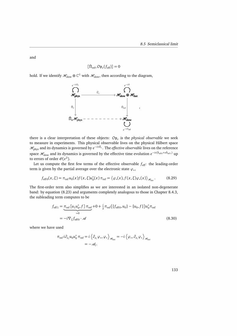
8.5 Semiclassical limit
and
[Πref,Opε( feff)] = 0
hold. If we identifyHslow ⊗C1 withHslow, then according to the diagram,
Hphys Hslow ⊗HfastUε //Hphys
ΠεHphys
Πε
Hslow ⊗Hfast
Hslow
Πref
ΠεHphys Hslow//__________
Hphys
e−i t Hε
Hslow ⊗Hfast
e−i th
Hslow
e−i theff
GG
,
there is a clear interpretation of these objects: Opε is the physical observable we seekto measure in experiments. This physical observable lives on the physical Hilbert spaceHphys and its dynamics is governed by e−i t Hε . The effective observable lives on the reference
spaceHslow and its dynamics is governed by the effective time evolution e−i t(heff 0+εheff 1) upto errors of order O (ε2).
Let us compute the first few terms of the effective observable feff: the leading-orderterm is given by the partial average over the electronic state ϕ∗,
feff 0(x ,ξ) = πref u0(x) f (x ,ξ)u∗0(x)πref =
ϕ∗(x), f (x ,ξ)ϕ∗(x)
Hfast. (8.29)
The first-order term also simplifies as we are interested in an isolated non-degenerateband: by equation (8.23) and arguments completely analogous to those in Chapter 8.4.3,the subleading term computes to be
feff 1 = πref [u1u∗0, f ]πref︸ ︷︷ ︸
=0
+0+ i2πref
feff 0, u0 − u0, f
u∗0πref
=−i∇ξ feff 0 · A (8.30)
where we have used
πref i∂x lu0u∗0πref = i
¬
∂x lϕ∗,ϕ∗
Hfast=−i
¬
ϕ∗,∂x lϕ∗
Hfast
=−Al .
133

8 Theory of multiscale systems
Example Two exceptionally important observables are our effective building block observ-ables
xeff := πref u]x]u∗πref = x +O (ε2) (8.31)
ξeff := πref u]ξ]u∗πref = ξ− εA (x) +O (ε2).
At least up to errors of order O (ε2) they look like the usual position observable and kineticmomentum associated to the “magnetic” field εΩl j := ∂x l
(εA j)− ∂x j(εAl). Since there
is a prefactor of ε, this means, the “magnetic” field is weak. It is not surprising that thispseudomagnetic field εΩ appears on the level of the classical equations of motion if weincrease our precision to include terms of O (ε).
Let us define the map Tε : Ξ−→ Ξ,
Tε : (x ,ξ) 7→
x ,ξ− εA (x)
+O (ε2)
which replaces (x ,ξ) by the effective observables
xeff,ξeff
=
x ,ξ− εA (x)
. This isin fact akin to adding a magnetic field to classical mechanics by minimal substitution,i. e. replacing momentum ξ with kinetic momentum ξ− A(x). We propose the following
Lemma 8.5.2 Let f be a macroscopic observable. Then up to errors of order O (ε2), feff isequal to the minimally substituted observable πref u0( f Tε)u∗0πref,
feff(x ,ξ) = ( f Tε)(x ,ξ) +O (ε2) = f
x ,ξ− εA (x)
+O (ε2). (8.32)
Proof We Taylor expand f Tε around ε = 0 and get
( f Tε)(x ,ξ) = f
x +O (ε2),ξ− εA (x) +O (ε2)
= f (x ,ξ)− ε∇ξ f (x ,ξ) · A (x) +O (ε2).
If we multiply the above expression with πref u0 from the left and u∗0πref from the right, itcoincides with feff 0 + ε feff 1 as given by equations (8.29) and (8.30).
This means, f and feff are related by minimal substitution and averaging over the fastdegrees of freedom.
Theorem 8.5.3 (Semiclassical limit) Let f be a macroscopic observable. Then the fullquantum dynamics of a Born-Oppenheimer system for an isolated non-degenerate band E∗can be approximated by the flow φt generated by
0 id−id 0
xξ
=
∇x
∇ξ
12ξ2 + E∗(x)
(8.33)
in the following sense:
Πε
Fqm(t)− Fcl(t)
Πε := Πεe+i t
εHεOpε( f )e
−i tε
Hε Πε − u∗0 Πref Opε( feff 0 φt) Πref u0
= O (ε2) (8.34)
134

8.5 Semiclassical limit
Proof First of all, from Chapter 8.4.4 (equation (8.28)), we know we can replace the fulldynamics e−i t
ε Πε by
e−i tε
Hε = u∗0e−i tε(heff 0+εheff 1)Πref u0 +O (ε).
This can be plugged into
ΠεFqm(t)Πε =
u∗0e−i tε(heff 0+εheff 1)Πref u0 +O (ε)
∗Opε( f )·
·
u∗0e−i tε(heff 0+εheff 1)Πref u0 +O (ε)
= u∗0e−i tε(heff 0+εheff 1) Πref u0 Opε( f ) u
∗0 Πref
︸ ︷︷ ︸
= feff 0+O (ε)
e−i tε(heff 0+εheff 1)u0 +O (ε)
= u∗0e−i tε(heff 0+εheff 1)Opε( feff 0)e
−i tε(heff 0+εheff 1)u0 +O (ε).
Now we make the semiclassical approximation: since we can regard Opε
heff 0 + εheff 1
and Opε( feff 0) as operators onHslow⊗C1 ∼=Hslow = L2(R3N ), we can invoke Theorem 7.1,the Egorov-type theorem: by the usual trick, we relate quantum and classical dynamics:first of all, since (xeff,ξeff) = (x ,ξ) + O (ε2), we can replace the effective variables byusual variables in the classical equations of motion, equation (8.33). We also see that thehamiltonian in these equations of motion is nothing but heff 0(x ,ξ) = 1
2ξ2 + E∗(x).
Now we can make a semiclassical argument to replace the full quantum mechanicsgenerated by heff 0 + εheff 1 and compare it to the quantization of the classically evolvedobservable,
e+i tε(heff 0+εheff 1)Opε( feff 0)e
−i tε(heff 0+εheff 1) −Opε( feff 0 φt) =
=
∫ t
0
dsd
ds
e+i sε(heff 0+εheff 1)Opε( feff 0 φt−s)e
−i sε(heff 0+εheff 1)
=
∫ t
0
ds e+i sε(heff 0+εheff 1)Opε
iε
heff 0 + εheff 1, feff 0(t − s)
]+
−d
dtfeff 0(t − s)
e−i sε(heff 0+εheff 1).
To show that the integral is small, we need to show that
iε
heff 0 + εheff 1, feff 0(t − s)
] −
heff 0, feff 0(t − s)
=
= iε
heff 0 + εheff 1, feff 0(t − s)
+O (ε)
is of order O (ε). In the single-band case, heff 0+εheff 1 and feff 0 are scalar-valued functionsand hence the pointwise commutator vanishes,
heff 0 + εheff 1, feff 0(t − s)
= 0.
135

8 Theory of multiscale systems
Thus, we have shown that equation (8.34) holds,
ΠεFqm(t)Πε = u∗0Πref Opε
feff φt
Πrefu0 +O (ε).
This concludes the proof.
The proof already contains the core idea how to push the error to O (ε2): one has tocompute heff 2 and then include the pseudomagnetic field εΩ in the semiclassical equationsof motion. However, since the pseudomagnetic field is weak, on our time scale and withour level of precision, it will not affect the dynamics.
136

Bibliography
[Arn89] V. I. Arnold. Mathematical Methods of Classical Mechanics. Springer, 1989.
[Arn92] V. I. Arnold. Ordinary Differential Equations. Springer, 1992.
[Ber75] F. A. Berezin. Quantization in complex symmetric spaces. Mathematics of theUSSR-Izvestiya, 9(2):341–379, 1975.
[Ber84] M. V. Berry. Quantal phase factors accompanying adiabatic changes. Proc. R.Soc. Lond. A, 392:45–57, 1984.
[BMK+03] A. Bohm, A. Mostafazadeh, H. Koizumi, Q. Niu, and J. Zwanziger. The Geo-metric Phase in Quantum Systems. Springer Verlag, 2003.
[Bui88] J Buitrago. A comment on the deduction of the dirac equation. EuropeanJournal of Physics, 9(2):149–150, 1988.
[Cor83] H. O. Cordes. A pseudodifferential Foldy-Wouthuysen transform. Communica-tions in Partial Differential Equations, 8(13):1475–1485, 1983.
[Cor04] H. O. Cordes. A precise pseudodifferential Foldy-Wouthuysen transform forthe Dirac equation. Journal of Evolution Equations, 4(1):128–138, March2004.
[Dre07] Michael Dreher. Dynamische systeme, 2007. Universität Konstanz.
[Ehr27] P. Ehrenfest. Bemerkung über die angenäherte Gültigkeit der klassischenMechanik innerhalb der Quantenmechanik. Zeitschrift für Physik, 455:455–457, 1927.
[FL08] Martin Fürst and Max Lein. Scaling Limits of the Dirac Equation with Slowly-varying Electromagnetic Fields: an Adiabatic Approach. to be published, 2008.
[FS10] Gero Friesecke and Bernd Schmidt. A sharp version of Ehrenfest’s theorem forgeneral self-adjoint operators. ArXiv e-prints, March 2010.
[FW50] Leslie L. Foldy and Siegfried A. Wouthuysen. On the dirac theory of spin 1/2particles and its non-relativistic limit. Phys. Rev., 78(1):29–36, Apr 1950.
137

Bibliography
[Hag80] George A. Hagedorn. Semiclassical Quantum Mechanics. Communications inMathematical Physics, 71:77–93, 1980.
[Kat66] Tosio Kato. Perturbation Theory for Linear Operators. Springer Verlag, 1966.
[KS04] Andreas Knauf and Rudi Seiler. Vorlesung mathematische physik i: Klassischemechanik, 2004. Universität Erlangen-Nürnberg.
[Lei05] Max Lein. A Dynamical Approach To Piezocurrents In Slowly Perturbed Crys-tals. diploma thesis, TU München, Munich, Germany, November 2005.
[Ler96] L Lerner. Derivation of the dirac equation from a relativistic representation ofspin. European Journal of Physics, 17(4):172–175, 1996.
[Lit86] Robert G. Littlejohn. The semiclassical evolution of wave packets. PhysicsReports, 138(4-5):193 – 291, 1986.
[LL01] Elliot Lieb and Michael Loss. Analysis. American Mathematical Society, 2001.
[LW93] Robert G. Littlejohn and Stefan Weigert. Diagonalization of multicompo-nent wave equations with a Born-Oppenheimer example. Physical Review A,47(5):3506–3512, 1993.
[MR99] Jerold E. Marsden and Tudor S. Ratiu. Introduction to mechanics and symme-try. Springer Verlag, New York, 1999.
[Mü99] M. Müller. Product rule for gauge invariant Weyl symbols and its applicationto the semiclassical description of guiding centre motion . J. Phys. A: Math.Gen., 32:1035–1052, 1999.
[PST03a] Gianluca Panati, Herbert Spohn, and Stefan Teufel. Effective dynamicsfor Bloch electrons: Peierls substitution . Communications in MathematicalPhysics, 242:547–578, October 2003.
[PST03b] Gianluca Panati, Herbert Spohn, and Stefan Teufel. Space Adiabatic Perturba-tion Theory. Adv. Theor. Math. Phys., 7:145–204, 2003.
[PST06] Gianluca Panati, Christof Sparber, and Stefan Teufel. A Simple Semi-classicalDescription Of Piezoelectricity. to be published, June 2006.
[PST07] Gianluca Panati, Herbert Spohn, and Stefan Teufel. The time-dependent born-oppenheimer approximation. M2AN, 41(2):297–314, March 2007.
[Rob87] Didier Robert. Autour de l’Approximation Semi-Classique. Birkhäuser, 1987.
138
Bibliography
[Rob98] D Robert. Semi-classical approximation in quantum mechanics. a survey ofold and recent results. Helvetica Physica Acta, 71(1):44–116, 1998.
[RS81] Michael Reed and Barry Simon. Methods of Modern Mathematical Physics, I:Functional Analysis. Academic Press, 1981.
[Sak94] Jun John Sakurai. Modern Quantum Mechanics. Addison Wesley PublishingCompany, 1994.
[Sim83] Barry Simon. Holonomy, the Quantum Adiabatic Theorem, and Berry’s Phase.Phys. Rev. Lett., 51(24):2167–2170, 1983.
[ST01] Herbert Spohn and Stefan Teufel. Adiabatic decoupling and time-dependentborn-oppenheimer theory. Comm. Math. Phys, 224:113–132, 2001.
[Teu03] Stefan Teufel. Adiabatic Perturbation Theory in Quantum Dynamics. SpringerVerlag, 2003.
[Tha92] Bernd Thaller. The Dirac Equation. Springer Verlag, 1992.
[Wal08] Stefan Waldmann. Poisson-Geometrie und Deformationsquantisierung. Eine Ein-führung. Springer Verlag, 2008.
[Wer05] Dirk Werner. Funktionalanalysis. Springer, 2005.
[Wig39] E. Wigner. On Unitary Representations of the Inhomogeneous Lorentz Group.The Annals of Mathematics, 40(1):149–204, 1939.
[Wya05] Robert E. Wyatt. Quantum dynamics with trajectories: introduction to quantumhydrodynamics. Springer, 2005.
[Ynd96] Francisco Yndurain. Relativistic Quantum Mechanics and Introduction to FieldTheory. Springer Verlag, 1996.
139