lecture machine learning neural networks - university of …€¦ · · 2012-02-06cs4442/9542b...

CS4442/9542bArtificial Intelligence IIprof. Olga Veksler

Lecture 5Machine Learning

Neural Networks

Many presentation Ideas are due to Andrew NG

Outline

• Motivation• Non linear discriminant functions

• Introduction to Neural Networks• Inspiration from Biology

• History

• Perceptron

• Multilayer Perceptron

• Practical Tips for Implementation

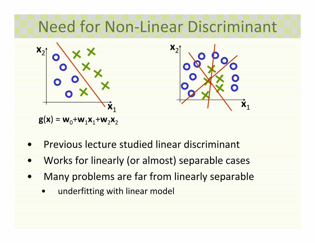
Need for Non‐Linear Discriminant

• Previous lecture studied linear discriminant

• Works for linearly (or almost) separable cases

• Many problems are far from linearly separable• underfitting with linear model

x1

x2

g(x) = w0+w1x1+w2x2

x1

x2


x1

x2

aZz

tp zaaJ

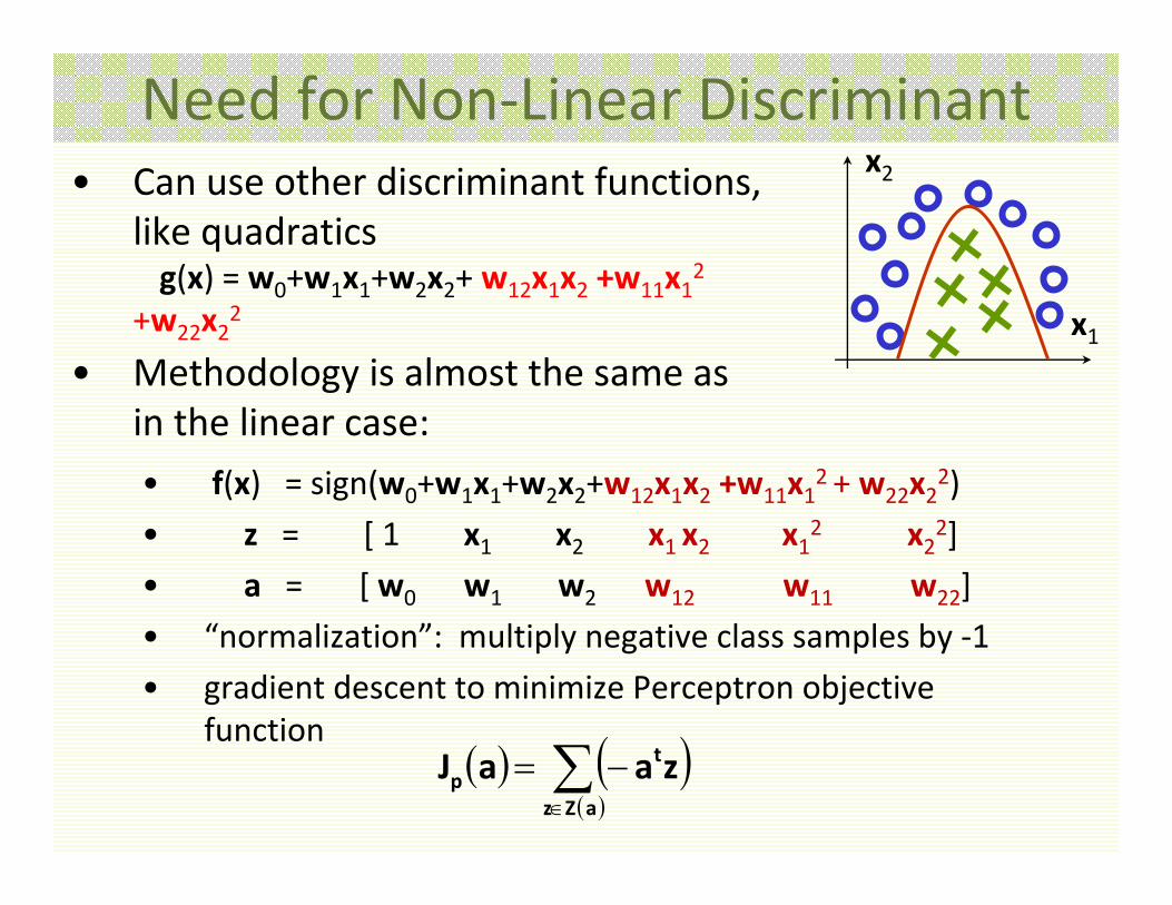
• Can use other discriminant functions, like quadraticsg(x) = w0+w1x1+w2x2+ w12x1x2 +w11x12

+w22x22

• Methodology is almost the same as in the linear case:• f(x) = sign(w0+w1x1+w2x2+w12x1x2 +w11x12 + w22x22)

• z = [ 1 x1 x2 x1 x2 x12 x22]

• a = [ w0 w1 w2 w12 w11 w22]

• “normalization”: multiply negative class samples by ‐1

• gradient descent to minimize Perceptron objective function


x1

x2• May need highly non‐linear decision boundaries

• This would require too many high order polynomial terms to fit

g(x) = w0+w1x1+w2x2++ w12x1x2 + w11x12 +w22x22 ++ w111x13+ w112x12x2 +w122x1x22 + w222x23 ++ even more terms of degree 4+ super many terms of degree k

• For n features, there O(nk) polynomial terms of degree k

• Many real world problems are modeled with hundreds and even thousands features

• 10010 is too large of function to deal with

Neural Networks

x1

x2• Neural Networks correspond to some discriminant function gNN(x)

• Can carve out arbitrarily complex decision boundaries without requiring so many terms as polynomial functions

• Neural Nets were inspired by research in how human brain works

• But also proved to be quite successful in practice

• Are used nowadays successfully for a wide variety of applications• took some time to get them to work

• now used by US post for postal code recognition

Neural Nets: Character Recognition• http://yann.lecun.com/exdb/lenet/index.html

7

Yann LeCun et. al.

Brain vs. Computer

• usually one very fast processor

• high reliability

• designed to solve logic and arithmetic problems

• absolute precision

• can solve a gazillion arithmetic and logic problems in an hour

• huge number of parallel but relatively slow and unreliable processors

• not perfectly precise, not perfectly reliable

• evolved (in a large part) for pattern recognition

• learns to solve various PR problems

seek inspiration for classification from human brain

One Learning Algorithm Hypothesis• Brain does many different things

• Seems like it runs many different “programs”

• Seems we have to write tons of different programs to mimic brain

• Hypothesis: there is a single underlying learning algorithm shared by different parts of the brain

• Evidence from neuro‐rewiring experiments

[Roe et al, 1992]

• Auditory cortex learns to see

• animals will eventually learn to perform a variety of object recognition tasks

• There are other similar rewiring experiments

• Route signal from eyes to the auditory cortex

• Cut the wire from ear to auditory cortex

Seeing with Tongue• Scientists use the amazing ability of the brain to learn to retrain brain tissue

• Seeing with tongue• BrainPort Technology

• Camera connected to a tongue array sensor

• Pictures are “painted” on the tongue• Bright pixels correspond to high voltage

• Gray pixels correspond to medium voltage

• Black pixels correspond to no voltage

• Learning takes from 2‐10 hours

• Some users describe experience resembling a low resolution version of vision they once had• able to recognize high contrast object, their location, movement tongue array

sensor

One Learning Algorithm Hypothesis

• Experimental evidence that we can plug any sensor to any part of the brain, and brain can learn how to deal with it

• Since the same physical piece of brain tissue can process sight,sound, etc.

• Maybe there is one learning algorithm can process sight, sound, etc.

• Maybe we need to figure out and implement an algorithm that approximates what the brain does

• Neural Networks were developed as a simulation of networks of neurons in human brain

Neuron: Basic Brain Processor

• Neurons (or nerve cells) are special cells that process and transmit information by electrical signaling• in brain and also spinal cord

• Human brain has around 1011 neurons

• A neuron connects to other neurons to form a network

• Each neuron cell communicates to anywhere from 1000 to 10,000 other neurons

Neuron: Main Components

13

dendrites

nucleus

cell body

axon

axon terminals

• cell body• computational unit

• dendrites• “input wires”, receive inputs from other neurons

• a neuron may have thousands of dendrites, usually short

• axon• “output wire”, sends signal to other neurons

• single long structure (up to 1 meter)

• splits in possibly thousands branches at the end, “axon terminals”

Neurons in Action (Simplified Picture)

• Cell body collects and processes signals from other neurons through dendrites

• If there the strength of incoming signals is large enough, the cell body sends an electricity pulse (a spike) to its axon

• This is the process by which all human thought, sensing, action, etc. happens

• Its axon, in turn, connects to dendrites of other neurons, transmitting spikes to other neurons

Artificial Neural Network (ANN) History: Birth

• 1943, famous paper by W. McCulloch (neurophysiologist) and W. Pitts (mathematician) • Using only math and algorithms, constructed a model of how neural

network may work

• Showed it is possible to construct any computable function with their network

• Was it possible to make a model of thoughts of a human being?

• Can be considered to be the birth of AI

• 1949, D. Hebb, introduced the first (purely pshychological) theory of learning• Brain learns at tasks through life, thereby it goes through tremendous

changes

• If two neurons fire together, they strengthen each other’s responses and are likely to fire together in the future

ANN History: First Successes

• 1958, F. Rosenblatt, • perceptron, oldest neural network still in use today

• that’s what we studied in lecture on linear classifiers

• Algorithm to train the perceptron network

• Built in hardware

• Proved convergence in linearly separable case

• 1959, B. Widrow and M. Hoff • Madaline

• First ANN applied to real problem

• eliminate echoes in phone lines

• Still in commercial use

ANN History: Stagnation• Early success lead to a lot of claims which were not fulfilled

• 1969, M. Minsky and S. Pappert• Book “Perceptrons”

• Proved that perceptrons can learn only linearly separable classes

• In particular cannot learn very simple XOR function

• Conjectured that multilayer neural networks also limited by linearly separable functions

• No funding and almost no research (at least in North America) in 1970’s as the result of 2 things above

ANN History: Revival• Revival of ANN in 1980’s

• 1982, J. Hopfield• New kind of networks (Hopfield’s networks)

• Not just model of how human brain might work, but also how to create useful devices• Implements associative memory

• 1982 joint US‐Japanese conference on ANN• US worries that it will stay behind

• Many examples of mulitlayer NN appear

• 1986, re‐discovery of backpropagation algorithm by Werbos, Rumelhart, Hinton and Ronald Williams• Allows a network to learn not linearly separable classes

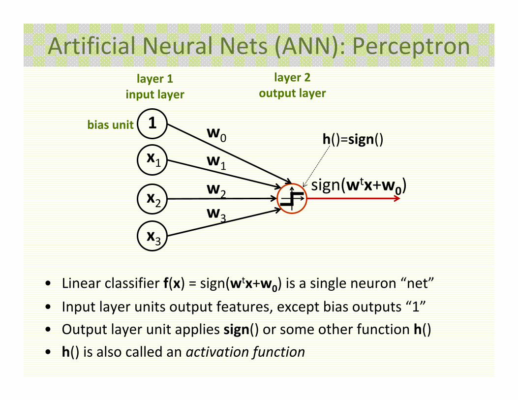
Artificial Neural Nets (ANN): Perceptron

• Linear classifier f(x) = sign(wtx+w0) is a single neuron “net”

x1

x2

x3

w1

w2

w3

sign(wtx+w0)

1 w0

layer 2output layer

layer 1input layer

bias unit

• Input layer units output features, except bias outputs “1”

• Output layer unit applies sign() or some other function h()

• h() is also called an activation function

h()=sign()

Multilayer Neural Network (MNN)

x1

x2

x3

1

layer 3output layer

layer 1Input layer

layer 2hidden layer

• First hidden unit outputs: h(…) = h(w0+w1x1 +w2x2 +w3x3)

w

w

h( w·h(…)+w·h(…) )

• Network corresponds to classifier f(x) = h( w·h(…)+w·h(…) )• More complex than Perceptron, more complex boundaries

• Second hidden unit outputs: h(…) = h(w0+w1x1 +w2x2 +w3x3)

MNN Small Example

x1

x2

1

layer 3: output layer 1: input layer 2: hidden

• Let activation function h() = sign()

• MNN Corresponds to classifier

f(x) = sign( 4h(…)+2h(…) + 7 )= sign(4sign(3x1+5x2)+2sign(6+3x2) + 7)

• MNN terminology: computing f(x) is called feed forward operation• graphically, function is computed from left to right

• Edge weights are learned through training

7

63

53

4

2

MNN: Multiple Classes

x1

x2

1

layer 1Input layer

layer 2hidden layer

• 3 classes, 2 features, 1 hidden layer• 3 input units, one for each feature

• 3 output units, one for each class

• 2 hidden units

• 1 bias unit, usually drawn in layer 1

layer 3output layer

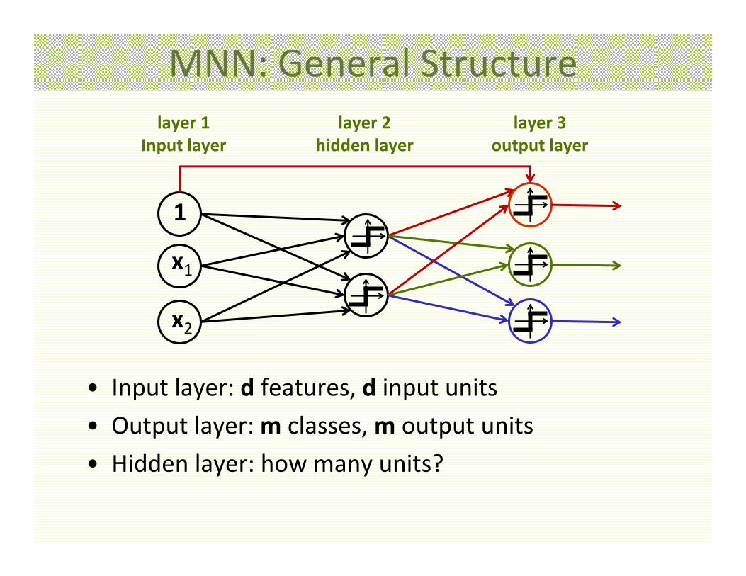
MNN: General Structure

x1

x2

1

layer 1Input layer

layer 2hidden layer

• Classification:

layer 3output layer

h(...)

h(...)

h(...)

• If f1(x) is largest, decide class 1



= f1(x)

• f(x) = [f1(x), f2(x), f3(x)] is multi‐dimensional

= f2(x)

= f3(x)


x1

x2

1

layer 1Input layer

layer 2hidden layer

• Input layer: d features, d input units

• Output layer: m classes, m output units

• Hidden layer: how many units?

layer 3output layer


x1

x2

1

layer 1Input layer

layer 2hidden layer

• Can have more than 1 hidden layer• ith layer connects to (i+1)th layer

• except bias unit can connect to any layer

• can have different number of units in each hidden layer

layer 4output layer

layer 3hidden layer

• First output unit outputs:

h(...) = h( wh(…) + w )

h(...)ww

w

w

= h( wh(wh(…) + wh(…)) + w )

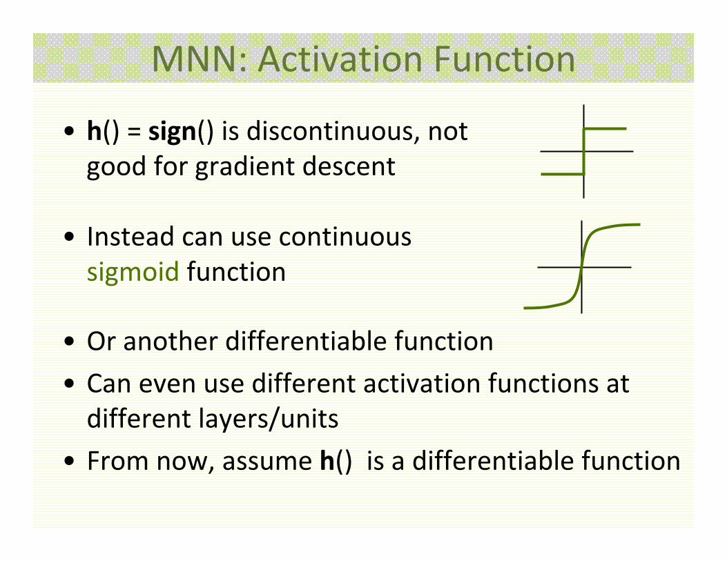
MNN: Activation Function

• h() = sign() is discontinuous, not good for gradient descent

• Instead can use continuous sigmoid function

• Or another differentiable function

• Can even use different activation functions at different layers/units

• From now, assume h() is a differentiable function

MNN: Overview• A neural network corresponds to a classifier f(x,w) that can be rather complex • complexity depends on the number of hidden layers/units

• f(x,w) is a composition of many functions• easier to visualize as a network

• notation gets ugly

• To train neural network, just as before• formulate an objective function J(w)

• optimize it with gradient descent

• That’s all!

• Except we need quite a few slides to write down details due to complexity of f(x,w)

Expressive Power of MNN• Every continuous function from input to output can be implemented with enough hidden units, 1 hidden layer, and proper nonlinear activation functions• easy to show that with linear activation function, multilayer

neural network is equivalent to perceptron

• This is more of theoretical than practical interest• Proof is not constructive (does not tell how construct MNN)

• Even if constructive, would be of no use, we do not know the desired function, our goal is to learn it through the samples

• But this result gives confidence that we are on the right track • MNN is general (expressive) enough to construct any required decision boundaries, unlike the Perceptron

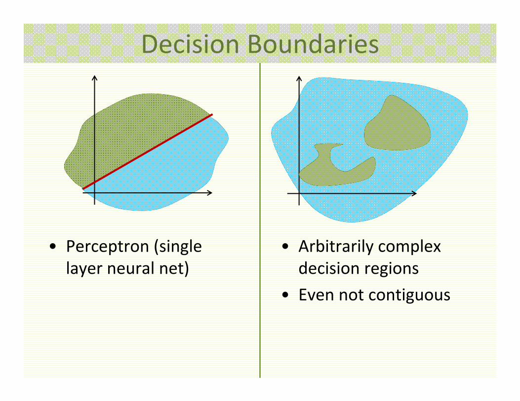
Decision Boundaries

• Perceptron (single layer neural net)

• Arbitrarily complex decision regions

• Even not contiguous

Nonlinear Decision Boundary: Example• Start with two Perceptrons, h() = sign()

x1

x2

1 ‐1‐1

1

– x1 + x2 – 1 > 0 class 1

x1

x2

1 ‐3‐1

1

– x1 + x2 – 3 > 0 class 1

x1

x2

‐1

1x1

x2

‐3

3

Nonlinear Decision Boundary: Example

x1

x2

1 ‐1‐11‐3‐11

• Now combine them into a 3 layer NN

1.5

1

1

x1

x2

‐1

1x1

x2

‐3

3+ x1

x2

‐3

3

1

‐1

• For Neural Networks, due to historical reasons, training and testing stages have special names

• Backpropagation (or training) Minimize objective function with gradient descent

• Feedforward (or testing)

MNN: Modes of Operation

MNN: Notation for Edge Weights

• wkpj is edge weight from unit p in layer k‐1 to unit j in layer k

1

x1

xd

….

layer 1input

….

layer 2hidden

….

layer k‐1hidden

bias unit or unit 0

unit 1

unit d

wk1m

• wk0j is edge weight from bias unit to unit j in layer k

wk0m

• wkj is all weights to unit j in layer k, i.e. wk

0j , wk1j , …, wk

N(k‐1)j

• N(k) is the number of units in layer k, excluding the bias unit

….

layer koutput

MNN: More Notation

x1

x2

1

layer 1 layer 2 layer 3

• For the input layer (k=1), z10 = 1 and z1j = xj, j ≠ 0

• Denote the output of unit j in layer k as zkj

• Convenient to set zk0 = 1 for all k

• Set zk = [zk0 , zk1,…, zkN(k)]

z32 = h(…)

z10 = 1

z12 = x2

• For all other layers, (k > 1), zkj = h(…)

z22 = h(…)

MNN: More Notation

x1

x2

1

layer 1 layer 2 layer 3

• Net activation at unit j in layer k > 1 is the sum of inputs

1

10

1kN

p

kj

kpj

kp

kj wwza

z1 1 w211

z10w201

z1 2 w2 21

• For k > 1, zkj = h(akj )

kkjwz 1

1

0

1kN

p

kpj

kp wz

221

12

211

11

201

10

21 wzwzwza

MNN: Class Representation• m class problem, let Neural Net have t layers

• Let xi be a example of class c

• It is convenient to denote its label as yi= row c

0

1

0

• Recall that ztc is the output of unit cin layer t (output layer)

• f(x)= zt= . If xi is of class c, want zt =

tm

tc

t

z

z

z

1

0

1

0

row c

• Want to minimize difference between yi and f(xi)

• Use squared difference

• Let w be all edge weights in MNN collected in one vector

Training MNN: Objective Function

n

i

m

c

ic

ic yxfwJ

1 1

2

21• Error on all examples:

• Gradient descent:

m

c

ic

ici yxfwJ

1

2

21• Error on one example xi :

initialize w to randomchoose , while ||J(w)|| >

w = w ‐ J(w)

• For simplicity, first consider error for one example xi

Training MNN: Single Sample

• Compute partial derivatives w.r.t. wkpj for all k, p, j

• Suppose have t layers

m

c

ic

ic

iii yxfxfywJ

1

22

21

21

• fc(xi) depends on w

• yi is independent of w

tcttc

tc

ic wzhahzxf 1

Training MNN: Single Sample

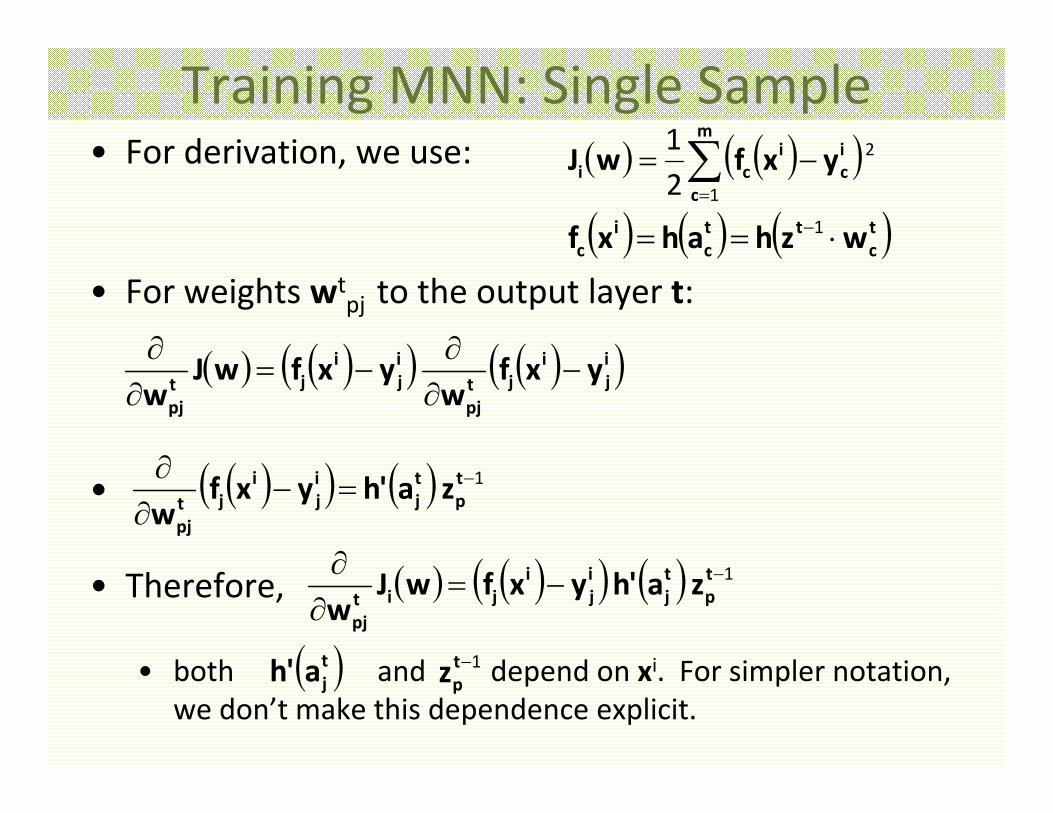
• For weights wtpj to the output layer t:

ijijt

pj

ij

ijt

pj

yxfw

yxfwJw

m

c

ic

ici yxfwJ

1

2

21

1 t

ptj

ij

ijit

pj

za'hyxfwJw

• 1 t

ptj

ij

ijt

pj

za'hyxfw

• Therefore,

• For derivation, we use:

tcttc

ic wzhahxf 1

• both and depend on xi. For simpler notation, we don’t make this dependence explicit.

tja'h 1tpz

Training MNN: Single Sample• For a layer k, compute partial derivatives w.r.t. wk

pj

• Gets complex, since have lots of function compositions

• Will give the rest of derivatives

• First define ekj, the error attributed to unit j in layer k:

• For layer t (output):

1 k

pkj

kjik

pj

za'hewJw

ijij

tj yxfe

• For layers k < t:

• Thus for 2 ≤ k ≤ t:

11

1

1

1

kjc

kc

kN

c

kc

kj wa'hee

MNN Training: Multiple Samples

n

i

m

c

ic

ic yxfwJ

1 1

2

21

• Error on all examples:

m

c

ic

ici yxfwJ

1

2

21• Error on one example xi :

1 k

pkj

kjik

pj

za'hewJw

n

i

kp

kj

kjk

pj

za'hewJw 1

1

Training Protocols• Batch Protocol

• true gradient descent

• weights are updated only after all examples are processed

• might be slow to converge

• Single Sample Protocol• examples are chosen randomly from the training set

• weights are updated after every example

• converges faster than batch, but maybe to an inferior solution

• Online Protocol• each example is presented only once, weights update after each example presentation

• used if number of examples is large and does not fit in memory

• should be avoided when possible

MNN Training: Single Sample

initialize w to small random numberschoose , while ||J(w)|| >

for i = 1 to nr = random index from {1,2,…,n}deltapjk = 0 p,j,k

for k = t to 2

wkpj = wk

pj + deltapjk p,j,k

jyxfe rj

rj

tj

1 kp

kj

kjpjkpjk za'hedeltadelta

jwa'hee k

jckc

kN

c

kc

kj

1

1

MNN Training: Batch

initialize w to small random numberschoose , while ||J(w)|| >

for i = 1 to ndeltapjk = 0 p,j,k

for k = t to 2

wkpj = wk

pj + deltapjk p,j,k

jyxfe ij

ij

tj

1 kp

kj


jwa'hee k

jckc

kN

c

kc

kj

1

1

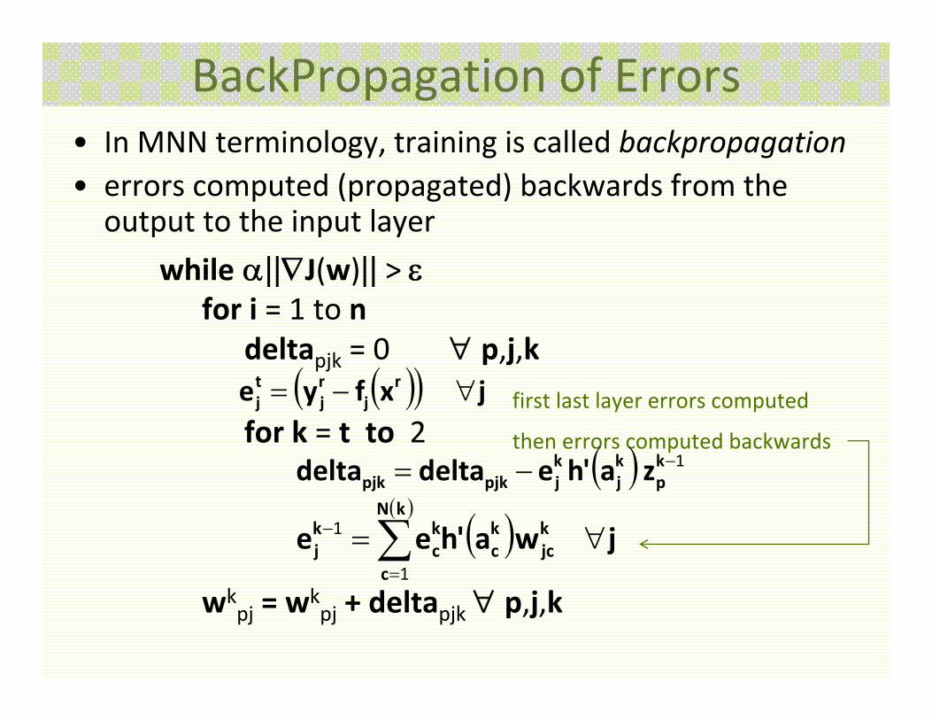
BackPropagation of Errors• In MNN terminology, training is called backpropagation• errors computed (propagated) backwards from the output to the input layer

first last layer errors computed

then errors computed backwards

while ||J(w)|| > for i = 1 to n

deltapjk = 0 p,j,k

for k = t to 2

wkpj = wk

pj + deltapjk p,j,k

jxfye rj

rj

tj

1 kp

kj


jwa'hee k

jckc

kN

c

kc

kj

1

1

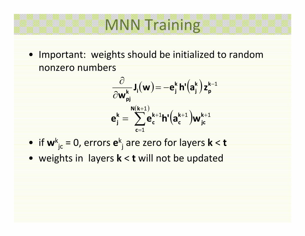
MNN Training

• Important: weights should be initialized to random nonzero numbers

• if wkjc = 0, errors ekj are zero for layers k < t

• weights in layers k < t will not be updated

1 k

pkj

kjik

pj

za'hewJw

11

1

1

1

kjc

kc

kN

c

kc

kj wa'hee

training time

Large training error:random decision regions in the beginning ‐ underfit

Small training error: decision regions improve with time

Zero training error: decision regions fit training data perfectly ‐ overfit

MNN Training: How long to Train?

can learn when to stop training through validation

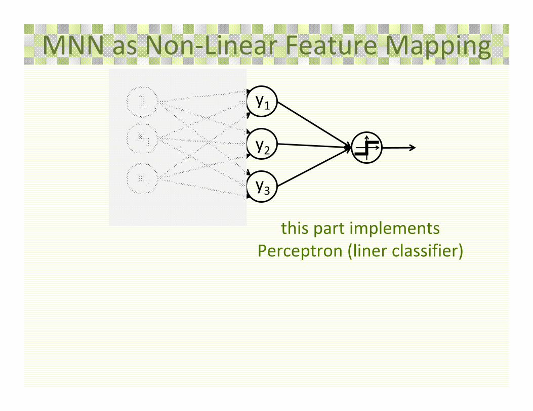
MNN as Non‐Linear Feature Mapping

x1

x2

1

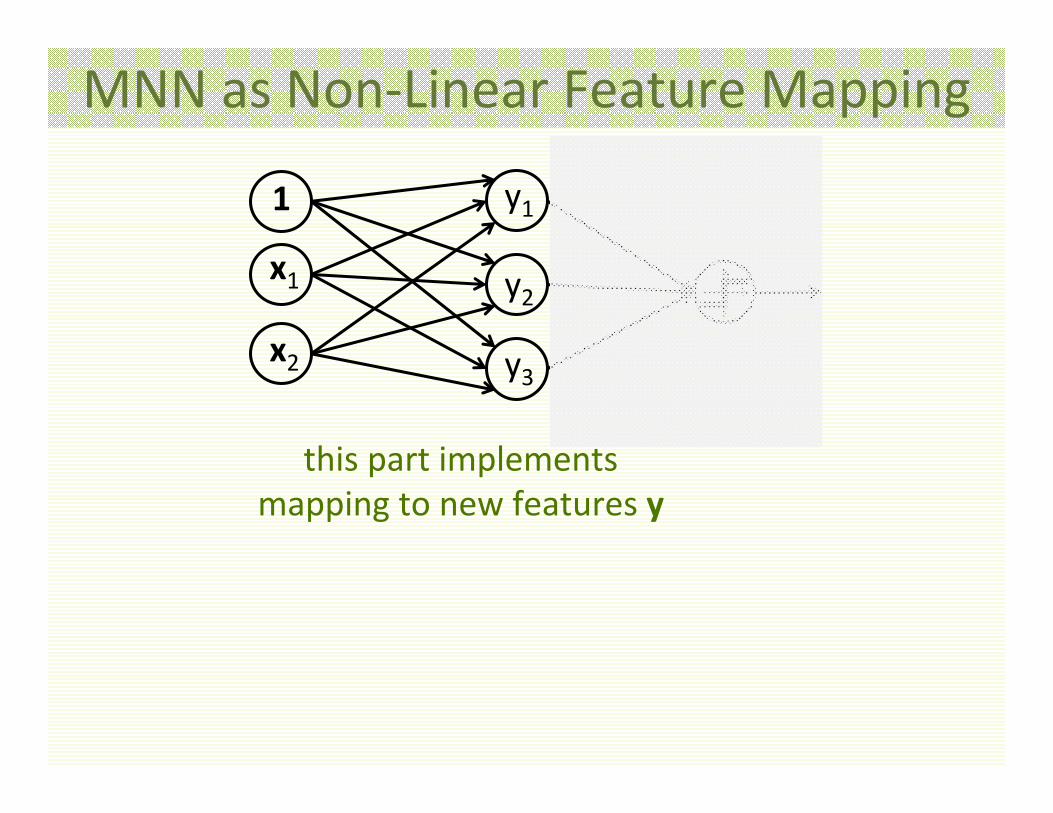
• MNN can be interpreted as first mapping input features to new features

• Then applying Perceptron (linear classifier) to the new features


x1

x2

1

this part implements Perceptron (liner classifier)

y1

y2

y3


x1

x2

1

this part implements mapping to new features y

y1

y2

y3

MNN as Nonlinear Feature Mapping

x1

x2

1 ‐1‐11‐3‐11

1.5

11

• Consider 3 layer NN example we saw previously:

x1

x2

non linearly separable in the original feature space

+

y1

y2

linearly separable in the new feature space

Neural Network Demo• http://www.youtube.com/watch?v=nIRGz1GEzgI

• To avoid overfitting, it is recommended to keep weights small

• Implement weight decay after each weight update:

wnew = wnew(1‐), 0 < < 1• Additional benefit is that “unused” weights grow small and may be eliminated altogether• a weight is “unused” if it is left almost unchanged by the backpropagation algorithm

Practical Tips: Weight Decay

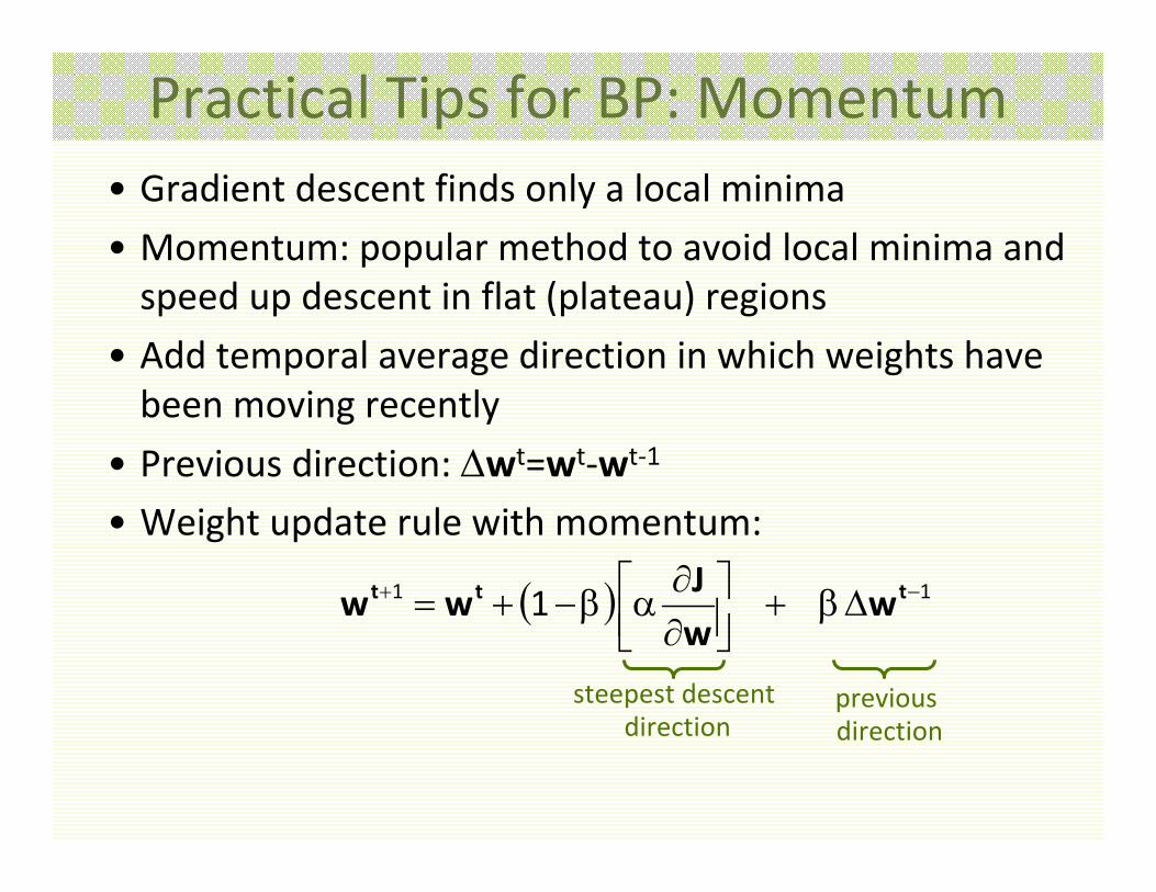
• Gradient descent finds only a local minima

• Momentum: popular method to avoid local minima and speed up descent in flat (plateau) regions

• Add temporal average direction in which weights have been moving recently

• Previous direction: wt=wt‐wt‐1

• Weight update rule with momentum:

Practical Tips for BP: Momentum

previous direction

steepest descent direction

11 1

ttt wwJ

ww

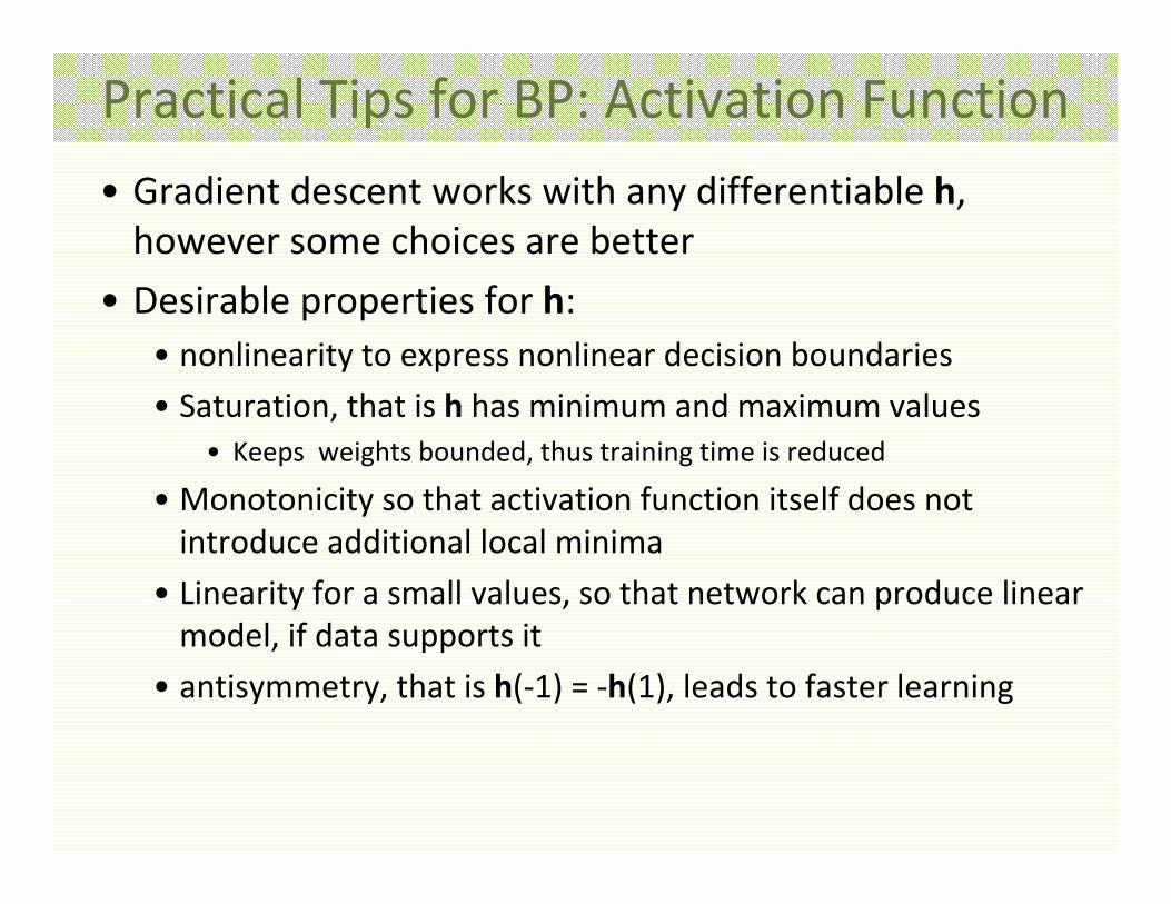
• Gradient descent works with any differentiable h, however some choices are better

• Desirable properties for h:• nonlinearity to express nonlinear decision boundaries

• Saturation, that is h has minimum and maximum values• Keeps weights bounded, thus training time is reduced

• Monotonicity so that activation function itself does not introduce additional local minima

• Linearity for a small values, so that network can produce linearmodel, if data supports it

• antisymmetry, that is h(‐1) = ‐h(1), leads to faster learning

Practical Tips for BP: Activation Function

• Sigmoid function h satisfies all of the properties

qbqb

qbqb

eeee

aqh

• Good parameter choices are a = 1.716, b = 2/3

• Linear range is roughly for –1 < q < 1

• Asymptotic values ±1.716• bigger than our labels, which are 1

• If asymptotic values were smaller than 1, training error will not be small

Practical Tips for BP: Activation Function

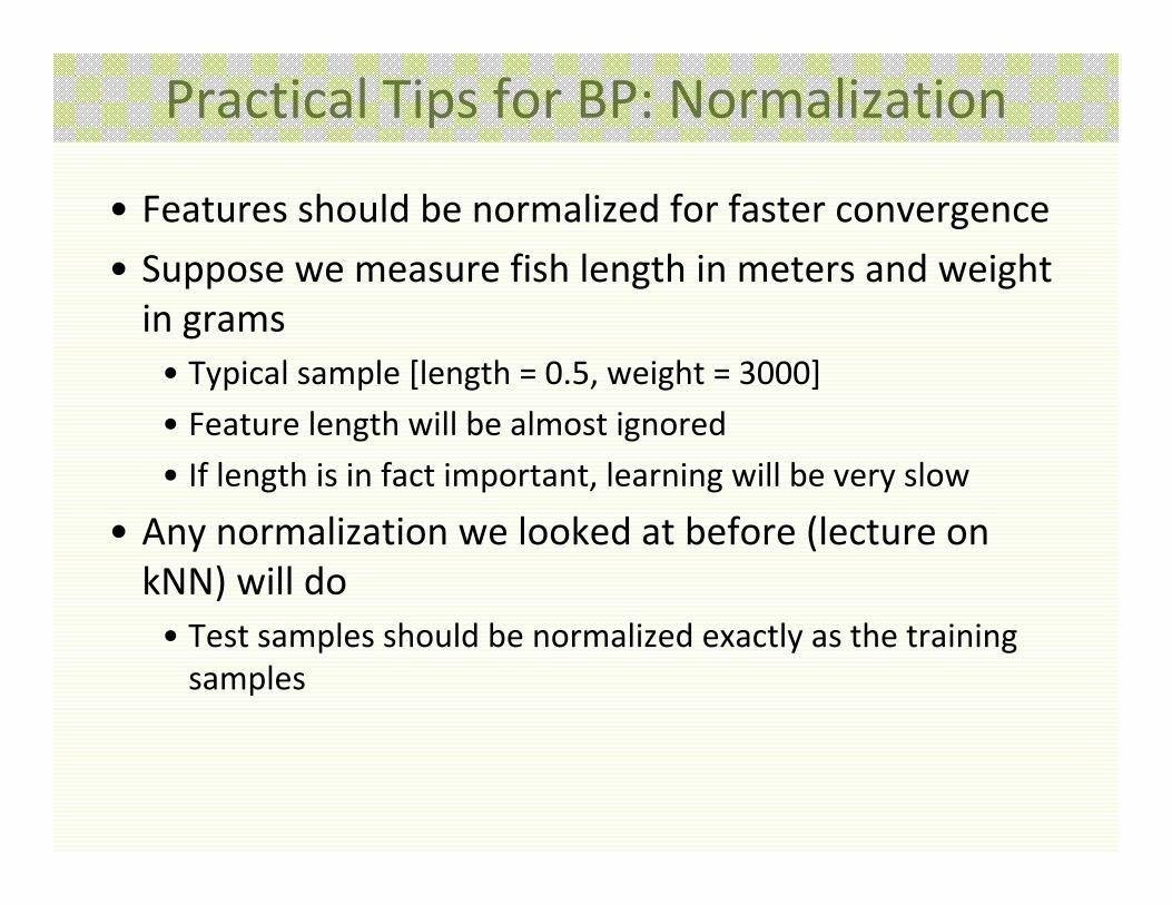
• Features should be normalized for faster convergence

• Suppose we measure fish length in meters and weight in grams• Typical sample [length = 0.5, weight = 3000]

• Feature length will be almost ignored

• If length is in fact important, learning will be very slow

• Any normalization we looked at before (lecture on kNN) will do• Test samples should be normalized exactly as the training samples

Practical Tips for BP: Normalization

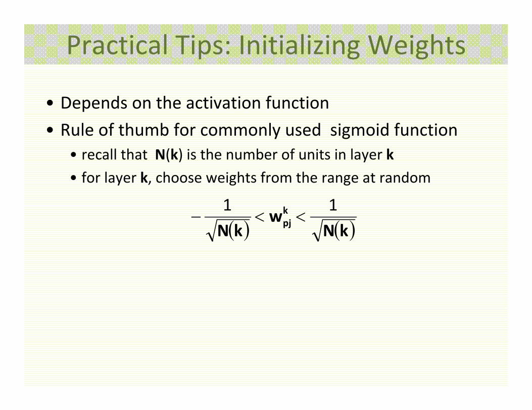
• Depends on the activation function

• Rule of thumb for commonly used sigmoid function• recall that N(k) is the number of units in layer k

• for layer k, choose weights from the range at random

kNw

kNkpj

11

Practical Tips: Initializing Weights

• As any gradient descent algorithm, backpropagationdepends on the learning rate

• Rule of thumb = 0.1

• However can adjust at the training time• The objective function J(w) should decrease during gradient descent

• If J(w) oscillates, is too large, decrease it

• If J(w) goes down but very slowly, is too small, increase it

Practical Tips: Learning Rate

Practical Tips for BP: # Hidden LayersPractical Tips: Number of Hidden Layers

• Network with 1 hidden layer has the same expressive power as with several hidden layers

• Having more than 1 hidden layer may result in faster learning and less hidden units

• However, networks with more than 1 hidden layer are more prone to stuck in a local minima

• Number of hidden units determines the expressive power of the network• Too small may not be sufficient to learn complex decision boundaries

• Too large may overfit the training data

• Sometimes recommended that • number of hidden units is larger than the number of input units

• number of hidden units is the same in all hidden layers

• Can choose number of hidden units through validation

Practical Tips for BP: Number of Hidden Units

• Advantages•MNN can learn complex mappings from inputs to outputs, based only on the training samples

• Easy to use

•Easy to incorporate a lot of heuristics

• Disadvantages• It is a “black box”, i.e. it is difficult to analyze and predict its behavior

•May take a long time to train

•May get trapped in a bad local minima

•A lot of tricks for best implementation

Concluding Remarks

lecture machine learning neural networks - university of …€¦ · · 2012-02-06cs4442/9542b...

Documents