Parallel Computer Architecture and Programming CMU 15-418/15-618, Spring 2017

Lecture 9:

Workload-Driven Performance Evaluation

CMU 15-418/618, Spring 2017

Nina Simone Feeling Good

(I Put a Spell on You)

Tunes

“72/72 on Assignment 2.”

- Nina SImone

CMU 15-418/618, Spring 2017

You are hired by [insert your favorite chip company here].

You walk in on day one, and your boss says “All of our senior architects have decided to take the year off. Your job is to lead the design of our next parallel processor.”

What questions might you ask?

CMU 15-418/618, Spring 2017

Your boss selects the application that matters most to the company “I want you to demonstrate good performance on this application.”

▪ Absolute performance? - Often measured as wall clock time - Another example: operations per second

▪ Speedup: performance improvement due to parallelism? - Execution time of sequential program / execution time on P processors - Operations per second on P processors / operations per second of sequential program

▪ Efficiency? - Performance per unit resource - e.g., operations per second per chip area, per dollar, per watt

How do you know if you have a good design?

CMU 15-418/618, Spring 2017

Measuring scaling▪ Consider the particle binning example from last week’s class

▪ Should speedup be measured against the performance of a parallel version of a program running on one processor, or the best sequential program?

1 320

5 764

9 11108

13 151412

0

12

4

5

3

CMU 15-418/618, Spring 2017

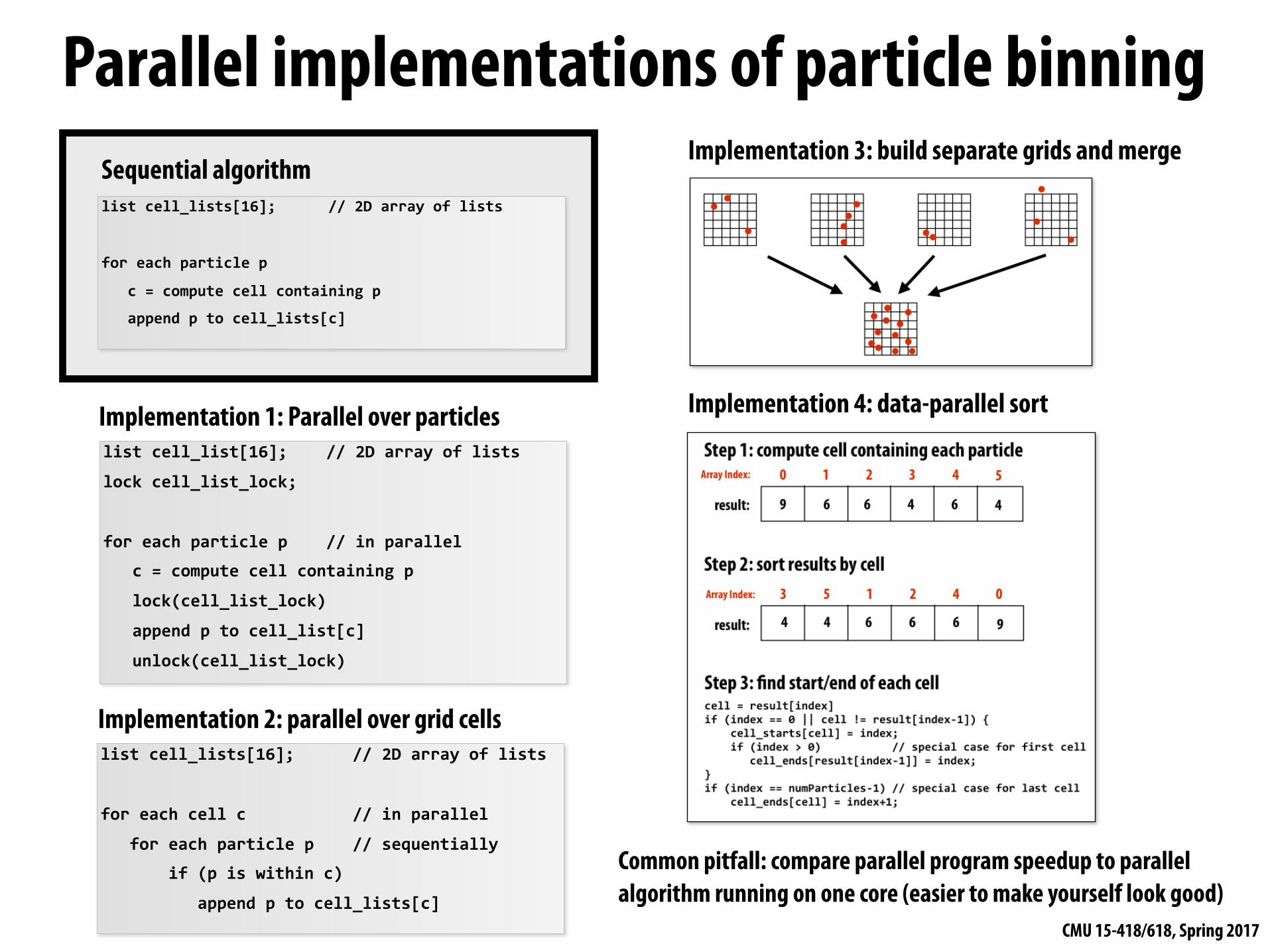
Parallel implementations of particle binning

listcell_lists[16];//2Darrayoflists

foreachcellc//inparallel

foreachparticlep//sequentially

if(piswithinc)

appendptocell_lists[c]

listcell_lists[16];//2Darrayoflists

foreachparticlep

c=computecellcontainingp

appendptocell_lists[c]

listcell_list[16];//2Darrayoflists

lockcell_list_lock;

foreachparticlep//inparallel

c=computecellcontainingp

lock(cell_list_lock)

appendptocell_list[c]

unlock(cell_list_lock)

Sequential algorithm

Implementation 1: Parallel over particles

Implementation 2: parallel over grid cells

Implementation 3: build separate grids and merge

Implementation 4: data-parallel sort

Common pitfall: compare parallel program speedup to parallel algorithm running on one core (easier to make yourself look good)

CMU 15-418/618, Spring 2017

Spee

dup

Processors

1 16842 32

Speedup of ocean sim application: 258 x 258 gridExecution on 32 processor SGI Origin 2000

Figure credit: Culler, Singh, and Gupta

CMU 15-418/618, Spring 2017

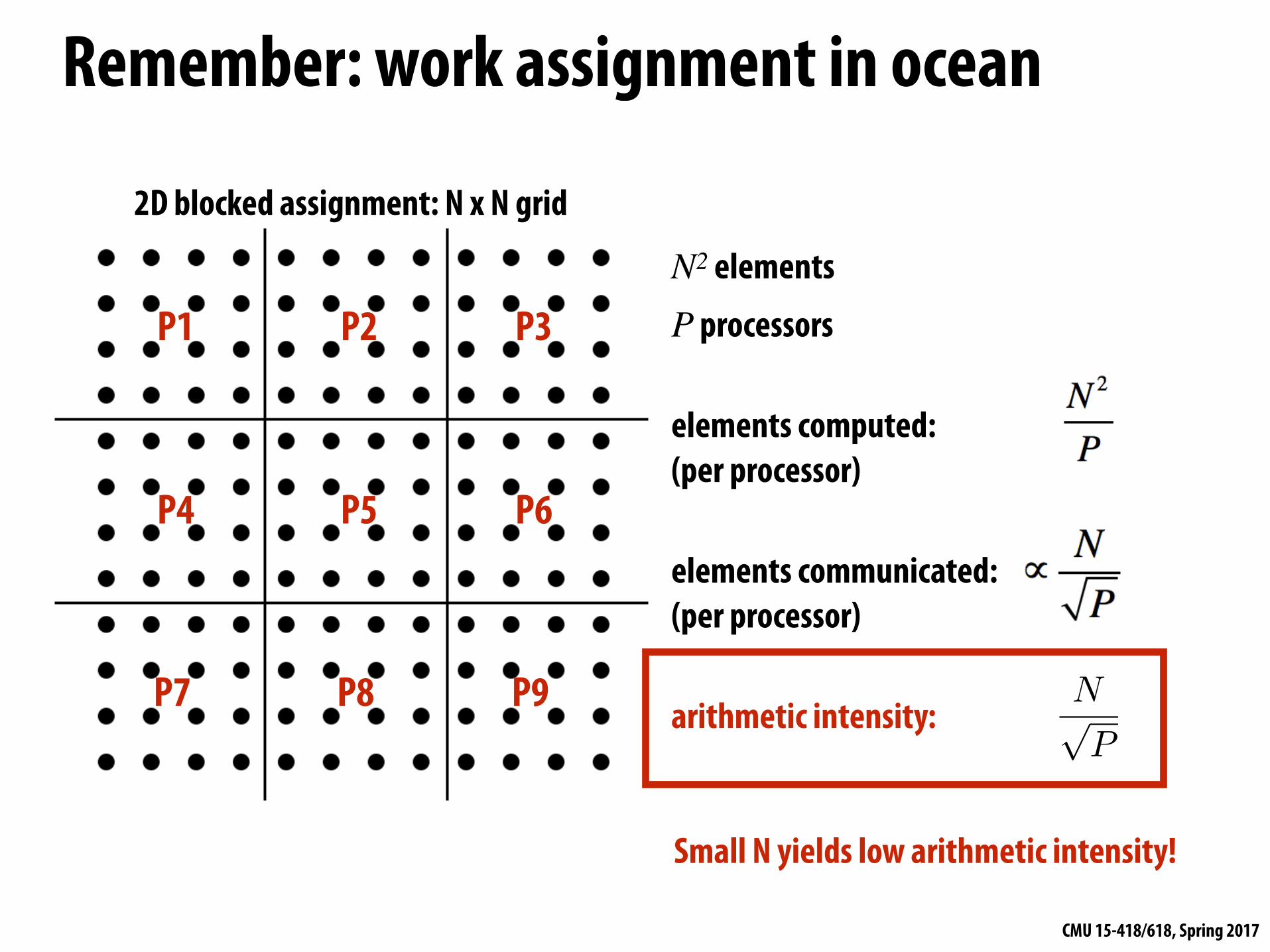
Remember: work assignment in ocean

P1 P2 P3

P4 P5 P6

P7 P8 P9

N2 elements

P processors

elements computed: (per processor)

elements communicated: (per processor) arithmetic intensity:

2D blocked assignment: N x N grid

Small N yields low arithmetic intensity!

NpP

CMU 15-418/618, Spring 2017

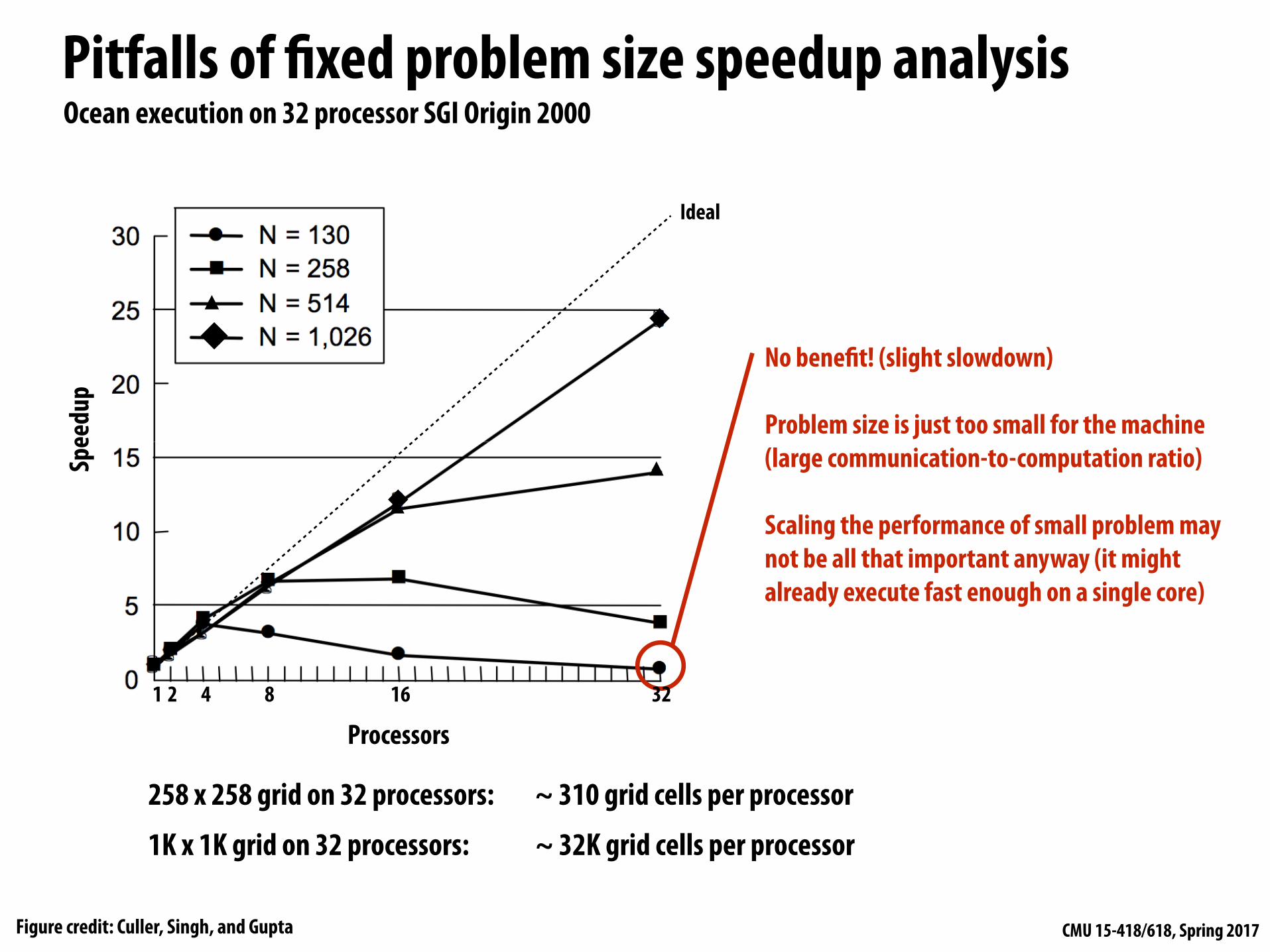
Pitfalls of fixed problem size speedup analysisSp

eedu

p

Processors

Ocean execution on 32 processor SGI Origin 2000

Ideal

258 x 258 grid on 32 processors: ~ 310 grid cells per processor

1K x 1K grid on 32 processors: ~ 32K grid cells per processor

No benefit! (slight slowdown)

Problem size is just too small for the machine (large communication-to-computation ratio)

Scaling the performance of small problem may not be all that important anyway (it might already execute fast enough on a single core)

1 3216842

Figure credit: Culler, Singh, and Gupta

CMU 15-418/618, Spring 2017

Pitfalls of fixed problem size speedup analysisSp

eedu

p

Processors1 32168

Execution on 32 processor SGI Origin 2000

Here: super-linear speedup! with enough processors, chunk of grid assigned to each processor begins to fit in cache (key working set fits in per-processor cache)

Another example: if problem size is too large for a single machine, working set may not fit in memory: causing thrashing to disk

(this would make speedup on a bigger parallel machine with more memory look amazing!)

42

Figure credit: Culler, Singh, and Gupta

CMU 15-418/618, Spring 2017

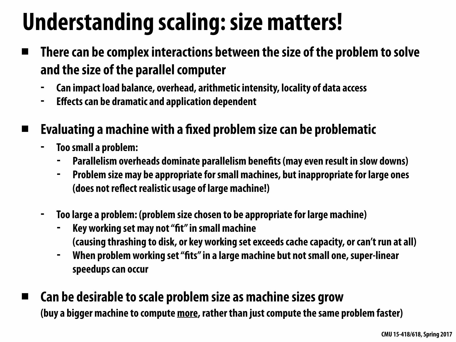
Understanding scaling: size matters!▪ There can be complex interactions between the size of the problem to solve

and the size of the parallel computer - Can impact load balance, overhead, arithmetic intensity, locality of data access - Effects can be dramatic and application dependent

▪ Evaluating a machine with a fixed problem size can be problematic - Too small a problem:

- Parallelism overheads dominate parallelism benefits (may even result in slow downs) - Problem size may be appropriate for small machines, but inappropriate for large ones

(does not reflect realistic usage of large machine!)

- Too large a problem: (problem size chosen to be appropriate for large machine) - Key working set may not “fit” in small machine

(causing thrashing to disk, or key working set exceeds cache capacity, or can’t run at all) - When problem working set “fits” in a large machine but not small one, super-linear

speedups can occur

▪ Can be desirable to scale problem size as machine sizes grow (buy a bigger machine to compute more, rather than just compute the same problem faster)

CMU 15-418/618, Spring 2017

Architects also think about scaling

▪ Scaling up: how does architecture’s performance scale with increasing core count? - Will design scale to the high end?

▪ Scaling down: how does architecture’s performance scale with decreasing core count? - Will design scale to the low end?

▪ Parallel architectures are designed to work in a range of contexts - Same architecture used for low-end, medium-scale, and high-end systems - GPUs are a great example

- Same SMM core architecture, different numbers of SMM cores per chip

A common question: “Does an architecture scale?”

Titan X: 24 SMM cores (250 watts)

GTX 980: 16 SMM cores (165 watts)

GTX 950: 6 SMM cores (90 watts)

Tegra X1: 2 SMM cores (mobile SoC)

CMU 15-418/618, Spring 2017

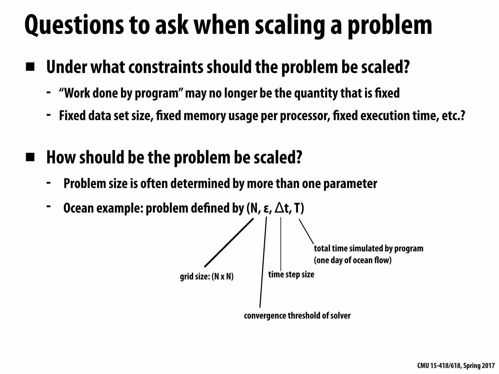
Questions to ask when scaling a problem▪ Under what constraints should the problem be scaled?

- “Work done by program” may no longer be the quantity that is fixed

- Fixed data set size, fixed memory usage per processor, fixed execution time, etc.?

▪ How should be the problem be scaled? - Problem size is often determined by more than one parameter

- Ocean example: problem defined by (N, ε, Δt, T)

grid size: (N x N)

convergence threshold of solver

time step size

total time simulated by program (one day of ocean flow)

CMU 15-418/618, Spring 2017

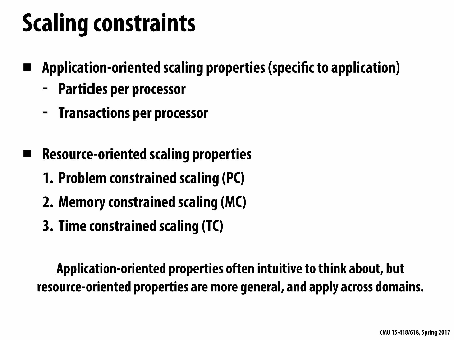
Scaling constraints

▪ Application-oriented scaling properties (specific to application) - Particles per processor - Transactions per processor

▪ Resource-oriented scaling properties 1. Problem constrained scaling (PC) 2. Memory constrained scaling (MC) 3. Time constrained scaling (TC)

Application-oriented properties often intuitive to think about, but resource-oriented properties are more general, and apply across domains.

CMU 15-418/618, Spring 2017

▪ Focus: use a parallel computer to solve the same problem faster

▪ Recall pitfalls from earlier in lecture (small problems may not be realistic workloads for large machines, big problems may not fit on small machines)

▪ Examples of problem-constrained scaling: - Almost everything we’ve considered parallelizing in class so far - Assignments 1 and 2

Problem-constrained scaling *

Speedup = time 1 processor

time P processors

* Problem-constrained scaling is often called “hard scaling”.

CMU 15-418/618, Spring 2017

Time-constrained scaling▪ Focus: completing more work in a fixed amount of time

- Execution time kept fixed as the machine (and problem) scales

▪ How to measure “work”? - Challenge: “work done” may not be linear function of problem inputs

(e.g. matrix multiplication is O(N3) work for O(N2) sized inputs) - One approach: “work done” is defined by execution time of same computation on a

single processor (but consider effects of thrashing if problem too big) - Ideally, a measure of work is:

- Simple to understand - Scales linearly with sequential run time (so ideal speedup remains linear in P)

Speedup = work done by P processors

work done by 1 processor

CMU 15-418/618, Spring 2017

Time-constrained scaling exampleReal-time 3D graphics: more compute power allows for rendering of much more complex scene Problem size metrics: number of polygons, texels sampled, shader length, etc.

Assassin's Creed Unity (2014)

Half Life 1 (1998)

Image credits: http://www.gamespot.com/forums/system-wars-314159282/assassin-s-creed-unity-best-graphics-of-2014-31696528/ http://www.game-weavers.com/?page_id=490

Half-Life (1998)

CMU 15-418/618, Spring 2017

Time-constrained scaling example

Large Synoptic Survey Telescope (LSST) - Estimated completion in 2019 - Acquire high-resolution survey of sky (3-gigapixel

image every 15 seconds, every night for many years)

Image credits: http://www.lsst.org http://mcdonaldobservatory.org

LSST will be located on top of Cerro Pachón Mountain, Chile

Rapid Image analysis compute platform (detect “potentially” interesting events)

Notify other observatories if potential event detected. Increasing compute capability allows

for more sophisticated detection algorithms (fewer false positives, detect broader class of events)

CMU 15-418/618, Spring 2017

More time-constrained scaling examples▪ Computational finance

- Run most sophisticated model possible in: 1 ms, 1 minute, overnight, etc.

▪ Modern web sites - Want to generate complex page, respond to user in X milliseconds

(studies show site usage directly corresponds to page load latency)

▪ Real-time computer vision for robotics - Consider self-driving car: want best-quality obstacle detection in 5 ms

CMU 15-418/618, Spring 2017

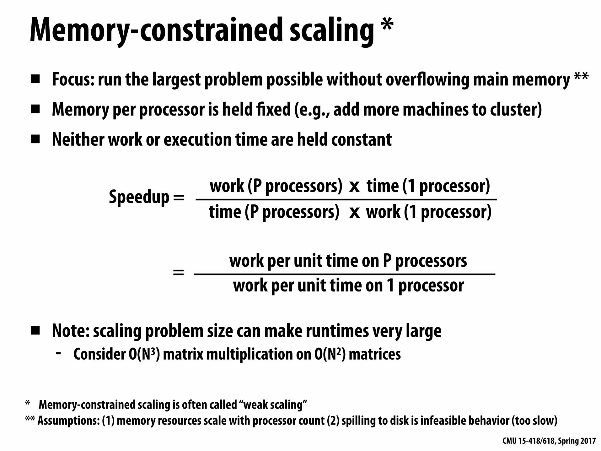
Memory-constrained scaling *▪ Focus: run the largest problem possible without overflowing main memory **

▪ Memory per processor is held fixed (e.g., add more machines to cluster)

▪ Neither work or execution time are held constant

▪ Note: scaling problem size can make runtimes very large - Consider O(N3) matrix multiplication on O(N2) matrices

* Memory-constrained scaling is often called “weak scaling” ** Assumptions: (1) memory resources scale with processor count (2) spilling to disk is infeasible behavior (too slow)

Speedup =

work per unit time on P processors work per unit time on 1 processor

work (P processors) x time (1 processor) time (P processors) x work (1 processor)

=

CMU 15-418/618, Spring 2017

Memory-constrained scaling examples▪ One motivation to use supercomputers and

large clusters is simply to be able to fit large problems in memory

▪ Large N-body problems - 2012 Supercomputing Gordon Bell Prize Winner:

1,073,741,824,000 particle N-body simulation on K-Computer (MPI implementation)

▪ Large-scale machine learning - Billions of clicks, documents, etc.

▪ Memcached (in memory caching system for web apps) - More servers = more available cache

Image credit: Ishiyama et al. 2012

2D domain decomposition of N-body simulation

CMU 15-418/618, Spring 2017

Scaling examples at PIXAR▪ Rendering a “shot” (a sequence of frames) in a movie

- Goal: minimize time to completion (problem constrained) - Assign each frame to a different machine in the cluster

▪ Artists working to design lighting for a scene - Provide interactive frame rate to artist (time constrained) - More performance = higher fidelity representation shown to artist in allotted time

▪ Physical simulation: e.g., fluid simulation - Parallelize simulation across multiple machines to fit simulation grid in aggregate

memory of processors (memory constrained)

▪ Final render of images for movie - Scene complexity is typically bounded by memory available on farm machines - One barrier to exploiting additional parallelism within a machine is that required

footprint often increases with number of processors (consider your implementation of assignment 2!)

CMU 15-418/618, Spring 2017

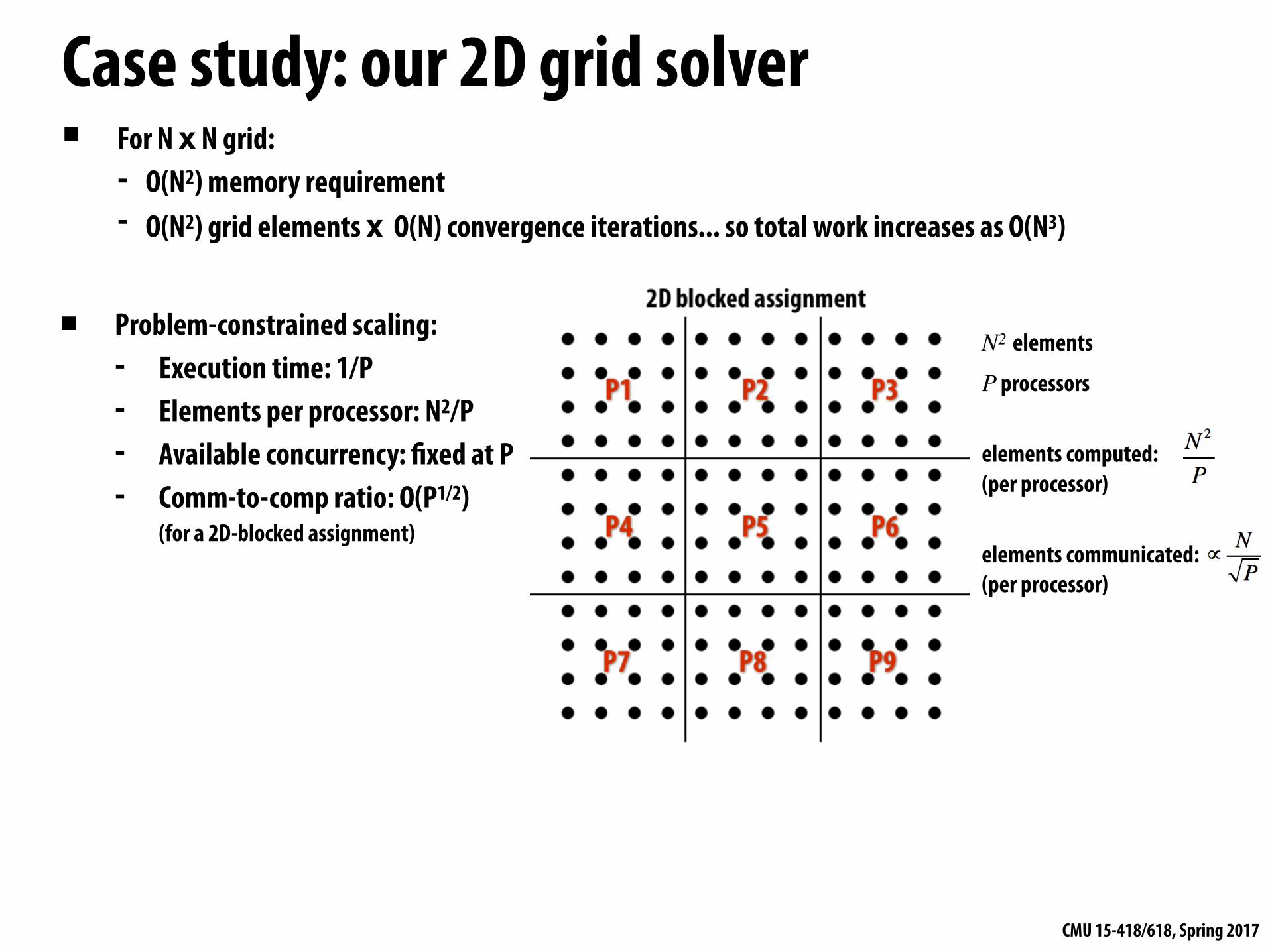
Case study: our 2D grid solver▪ For N x N grid:

- O(N2) memory requirement - O(N2) grid elements x O(N) convergence iterations... so total work increases as O(N3)

▪ Problem-constrained scaling: - Execution time: 1/P - Elements per processor: N2/P - Available concurrency: fixed at P - Comm-to-comp ratio: O(P1/2)

(for a 2D-blocked assignment)

N2 elements

P processors

elements computed: (per processor)

elements communicated: (per processor)

CMU 15-418/618, Spring 2017

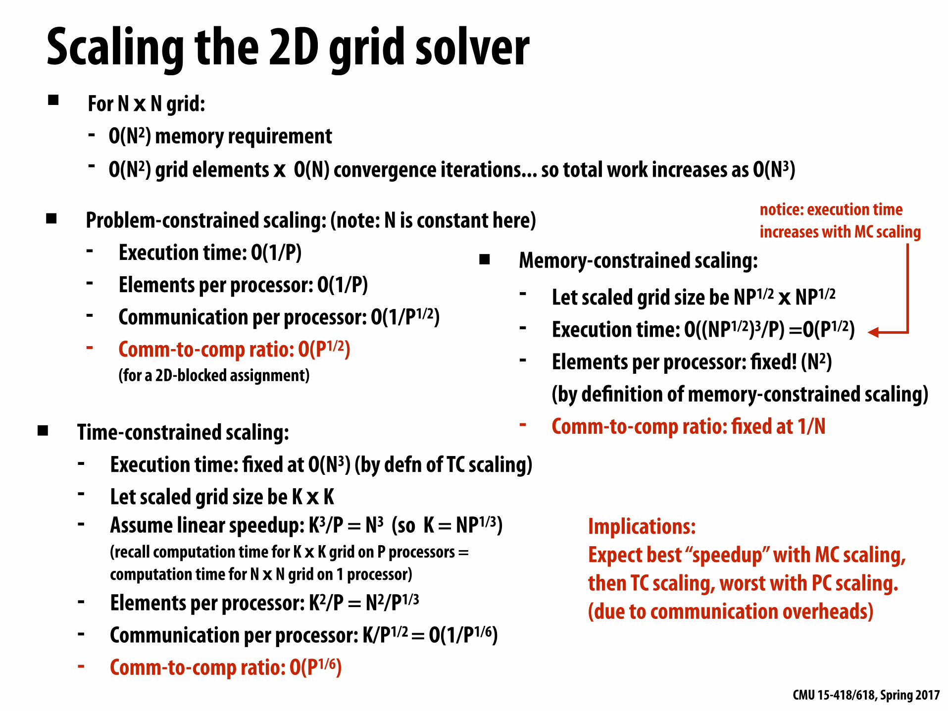
Scaling the 2D grid solver▪ For N x N grid:

- O(N2) memory requirement - O(N2) grid elements x O(N) convergence iterations... so total work increases as O(N3)

▪ Problem-constrained scaling: (note: N is constant here) - Execution time: O(1/P) - Elements per processor: O(1/P) - Communication per processor: O(1/P1/2) - Comm-to-comp ratio: O(P1/2)

(for a 2D-blocked assignment)

▪ Time-constrained scaling: - Execution time: fixed at O(N3) (by defn of TC scaling) - Let scaled grid size be K x K - Assume linear speedup: K3/P = N3 (so K = NP1/3)

(recall computation time for K x K grid on P processors = computation time for N x N grid on 1 processor)

- Elements per processor: K2/P = N2/P1/3

- Communication per processor: K/P1/2 = O(1/P1/6)

- Comm-to-comp ratio: O(P1/6)

▪ Memory-constrained scaling: - Let scaled grid size be NP1/2 x NP1/2 - Execution time: O((NP1/2)3/P) =O(P1/2) - Elements per processor: fixed! (N2)

(by definition of memory-constrained scaling) - Comm-to-comp ratio: fixed at 1/N

notice: execution time increases with MC scaling

Implications: Expect best “speedup” with MC scaling, then TC scaling, worst with PC scaling. (due to communication overheads)

CMU 15-418/618, Spring 2017

Word of caution about problem scaling

▪ Problem size in the previous examples was a single parameter n

▪ In practice, problem size is a combination of parameters - Recall Ocean example: problem is =(n, ε, Δt, T)

▪ Problem parameters are often related (not independent) - Example from Barnes-Hut: increasing particle count n changes required

simulation time step and force calculation accuracy parameter ϴ

▪ Must be cognizant of these relationships under situations of TC or MC scaling

CMU 15-418/618, Spring 2017

Scaling summary

▪ Performance improvement due to parallelism is measured by speedup

▪ But speedup metrics take different forms for different scaling models - Which model matters most is application/context specific

▪ In addition to assignment and orchestration, behavior of a parallel program depends significantly on the scaling properties of the problem and also the machine.

- When analyzing performance, be careful to analyze realistic regimes of operation (realistic sizes and realistic problem size parameters)

- This requires application knowledge

CMU 15-418/618, Spring 2017

You have an idea for how to design a parallel machine to meet the needs of your boss.

How are you going to test this idea?

Back to our example of your hypothetical future job...

CMU 15-418/618, Spring 2017

Evaluating an architectural idea: simulation

▪ Architects evaluate architectural decisions quantitatively using chip simulators - Let’s say an architect is considering adding a feature

- Architect runs simulations with new feature, runs simulations without new feature, compare simulated performance

- Simulate against a wide collection of benchmarks

▪ Design detailed simulator to test new architectural feature - Very expensive to simulate a parallel machine in full detail

- Often cannot simulate full machine configurations or realistic problem sizes (must scale down workloads significantly!)

- Architects need to be confident scaled down simulated results predict reality (otherwise, why do the evaluation at all?)

CMU 15-418/618, Spring 2017

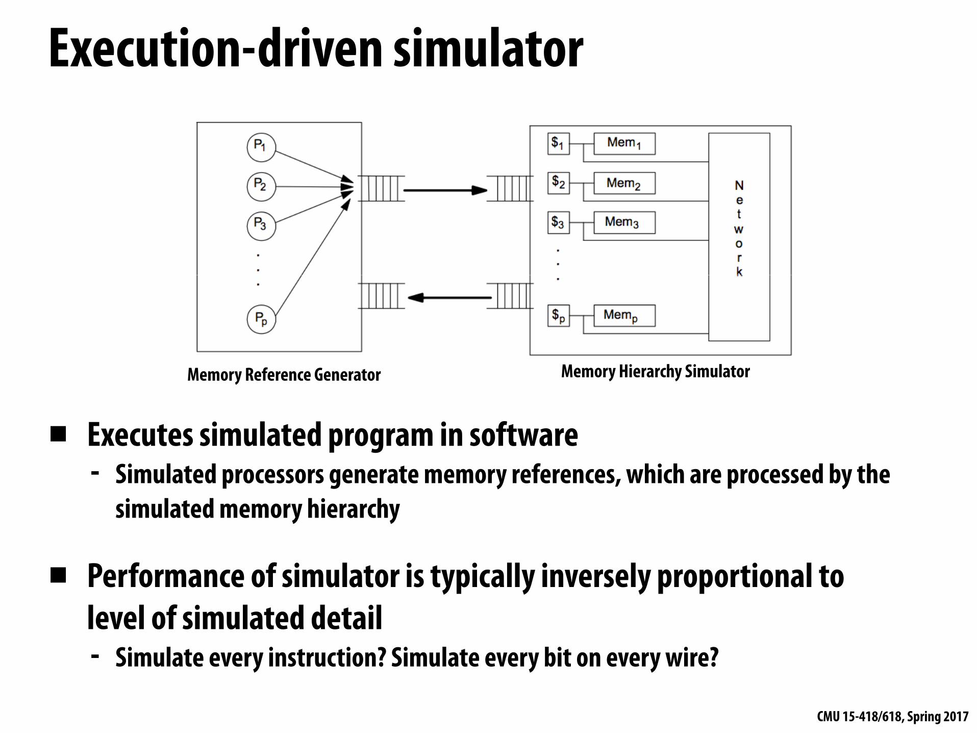
Execution-driven simulator

▪ Executes simulated program in software - Simulated processors generate memory references, which are processed by the

simulated memory hierarchy

▪ Performance of simulator is typically inversely proportional to level of simulated detail - Simulate every instruction? Simulate every bit on every wire?

Memory Reference Generator Memory Hierarchy Simulator

CMU 15-418/618, Spring 2017

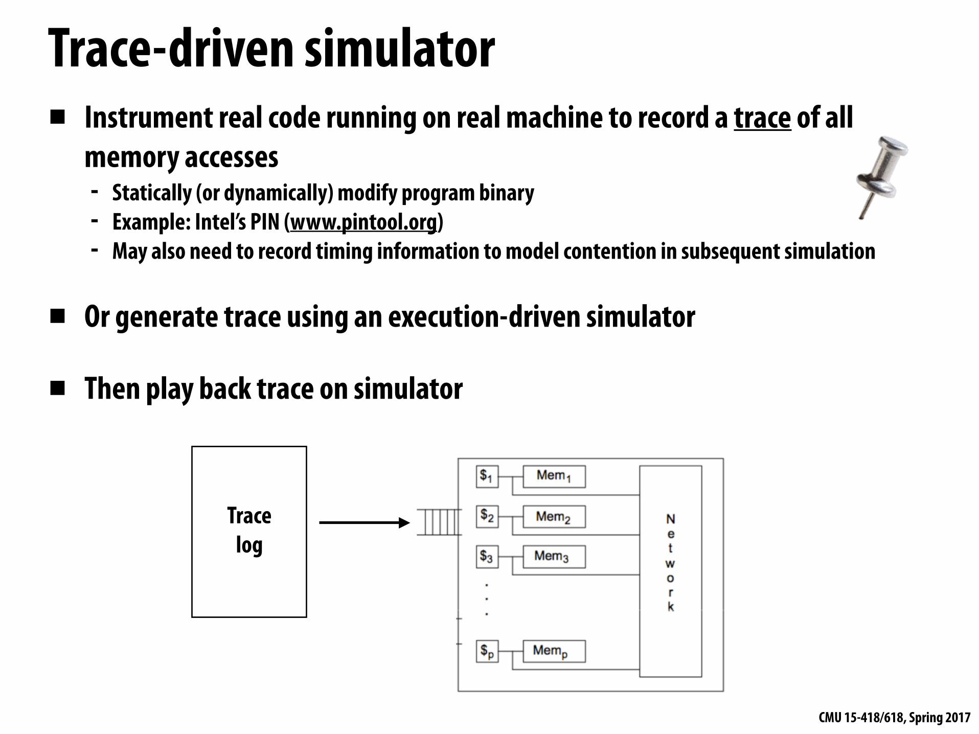
▪ Instrument real code running on real machine to record a trace of all memory accesses - Statically (or dynamically) modify program binary - Example: Intel’s PIN (www.pintool.org) - May also need to record timing information to model contention in subsequent simulation

▪ Or generate trace using an execution-driven simulator

▪ Then play back trace on simulator

Trace-driven simulator

Trace log

CMU 15-418/618, Spring 2017

Architectural simulation state space▪ Another evaluation challenge: dealing with large parameter space of machines

- Num processors, cache sizes, cache line sizes, memory bandwidths, etc.

Pareto Curve: (here: plots energy/perf trade-off)

Performance Density (ops/nS/mm2)

Ener

gy Pe

r Ope

ratio

n (n

J/op)

Maximum performance per unit chip area

(but high energy consumption)

High energy efficiency (but lower performance density)

CMU 15-418/618, Spring 2017

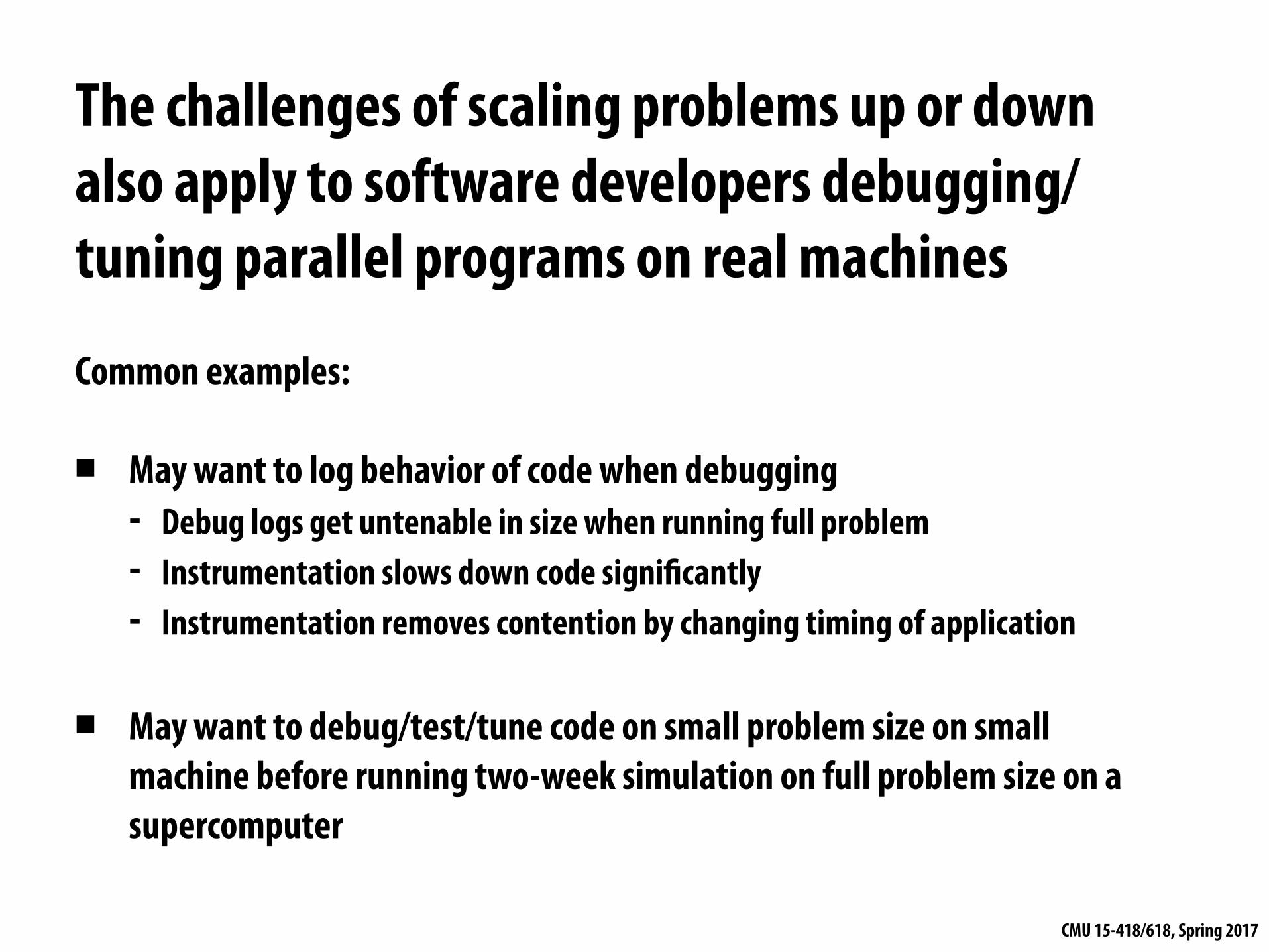
The challenges of scaling problems up or down also apply to software developers debugging/tuning parallel programs on real machines

Common examples:

▪ May want to log behavior of code when debugging - Debug logs get untenable in size when running full problem - Instrumentation slows down code significantly - Instrumentation removes contention by changing timing of application

▪ May want to debug/test/tune code on small problem size on small machine before running two-week simulation on full problem size on a supercomputer

CMU 15-418/618, Spring 2017

Example: scaling down assignment 2▪ Problem size = (w, h, num_circles, ...)

image width, height number of scene circles

Original image (w=8)

Smaller Image (1/2 size: w=4) Original image

(w=8)

width-4 crop of original image

Alternative solution: Render crop of full-size image

Shrink image, but keep circle data the same: - Ratio of circle/box “filtering” work to per-pixel work changes - With fixed tile size: number of circles in a tile changes

CMU 15-418/618, Spring 2017

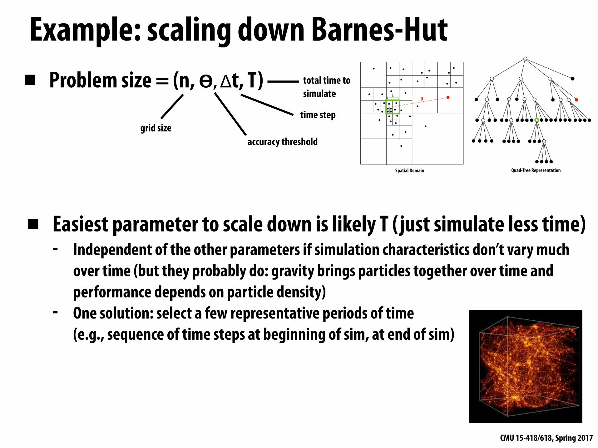
Example: scaling down Barnes-Hut▪ Problem size = (n, ϴ, Δt, T)

grid sizeaccuracy threshold

time step

total time to simulate

▪ Easiest parameter to scale down is likely T (just simulate less time) - Independent of the other parameters if simulation characteristics don’t vary much

over time (but they probably do: gravity brings particles together over time and performance depends on particle density)

- One solution: select a few representative periods of time (e.g., sequence of time steps at beginning of sim, at end of sim)

CMU 15-418/618, Spring 2017

Challenges of scaling down (or up)▪ Preserve ratio of time spent in different program phases

- Assignment 2: “bin circles” phase, process lists phase - Ray-trace and Barnes-Hut: both have tree build and tree traverse phases

- Shrinking screen size changes cost of tracing rays but not cost of building tree - Changing density of particles changes per particle cost in Barnes-Hut

▪ Preserve important behavioral characteristics - arithmetic intensity, load balance, locality, working set sizes - e.g., shrinking grid size in solver changes arithmetic intensity

▪ Preserve contention and communication patterns - Tough to preserve contention since contention is a function of timing and ratios

▪ Preserve scaling relationships between problem parameters - e.g., Barnes-Hut: scaling up particle count requires scaling down time step for

physics reasons

CMU 15-418/618, Spring 2017

There is simply no substitute for the experience of writing and tuning your own parallel programs. But today’s take-away is: BE CAREFUL!

It can be very tricky to evaluate and tune parallel software and parallel machines.

It can be very easy to obtain misleading results or tune code (or a billion dollar hardware design) for a workload that is not representative of real-world use cases.

It is helpful to start by precisely stating your application performance goals. Then determine if your evaluation approach is consistent with these goals.

CMU 15-418/618, Spring 2017

Here are some tricks for understanding the performance of parallel software

CMU 15-418/618, Spring 2017

Always, always, always try the simplest parallel solution first, then measure

performance to see where you stand.

CMU 15-418/618, Spring 2017

A useful performance analysis strategy

▪ Determine if your performance is limited by computation, memory bandwidth (or memory latency), or synchronization?

▪ Try and establish “high watermarks” - What’s the best you can do in practice? - How close is your implementation to a best-case scenario?

CMU 15-418/618, Spring 2017

Roofline model▪ Use microbenchmarks to compute peak performance of a machine as a function of

arithmetic intensity of application

▪ Then compare application’s performance to known peak values

Figure credit: Williams et al. 2009

horizontal region: compute limiteddiagonal region: memory bandwidth limited

CMU 15-418/618, Spring 2017

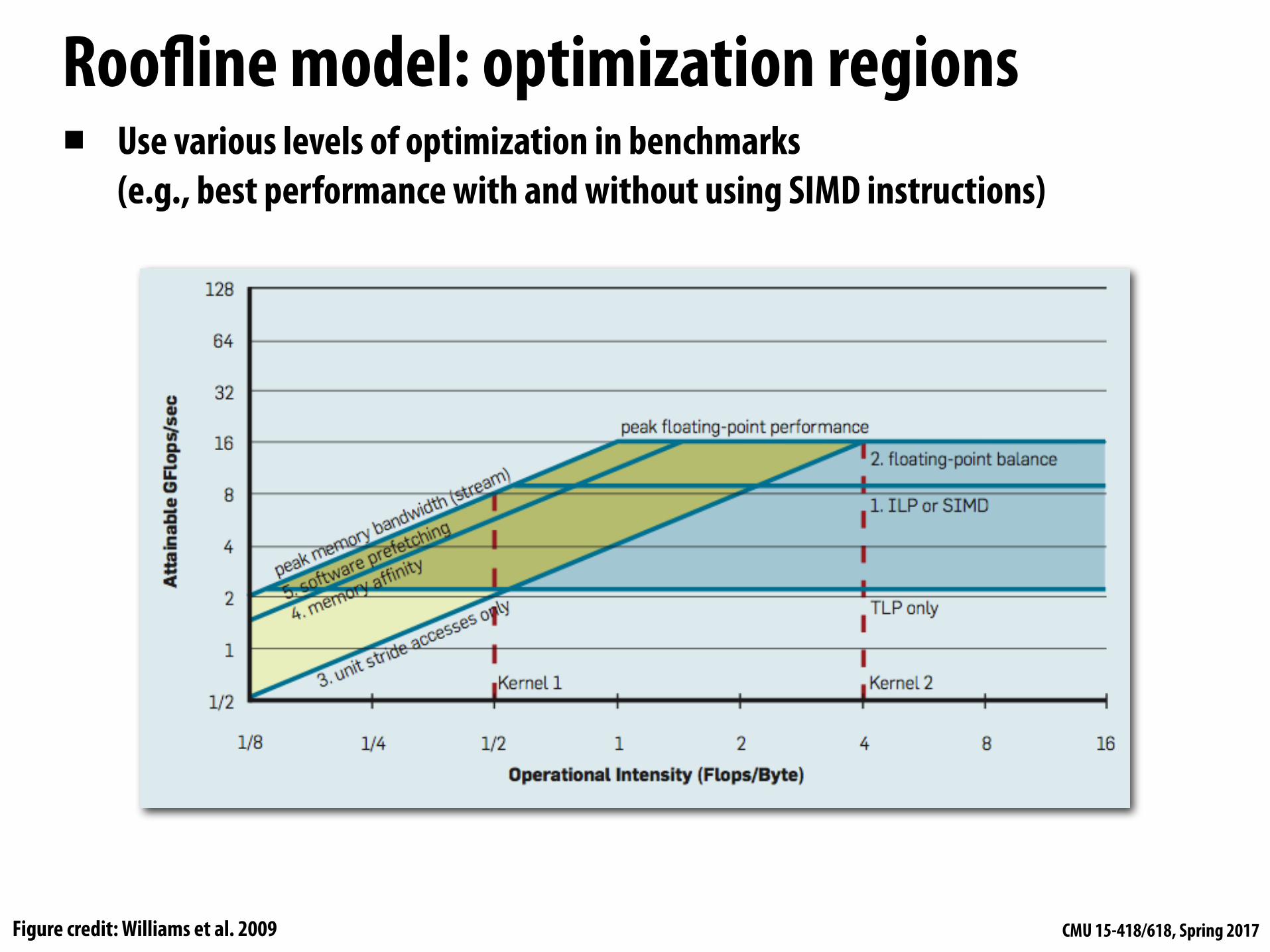
Roofline model: optimization regions▪ Use various levels of optimization in benchmarks

(e.g., best performance with and without using SIMD instructions)

Figure credit: Williams et al. 2009

CMU 15-418/618, Spring 2017

Establishing high watermarks *Add “math” (non-memory instructions) Does execution time increase linearly with operation count as math is added? (If so, this is evidence that code is instruction-rate limited)

Change all array accesses to A[0] How much faster does your code get? (This establishes an upper bound on benefit of improving locality of data access)

Remove all atomic operations or locks How much faster does your code get? (provided it still does approximately the same amount of work) (This establishes an upper bound on benefit of reducing sync overhead.)

Remove almost all math, but load same data How much does execution-time decrease? If not much, suspect memory bottleneck

* Computation, memory access, and synchronization are almost never perfectly overlapped. As a result, overall performance will rarely be dictated entirely by compute or by bandwidth or by sync. Even so, the sensitivity of performance change to the above program modifications can be a good indication of dominant costs

CMU 15-418/618, Spring 2017

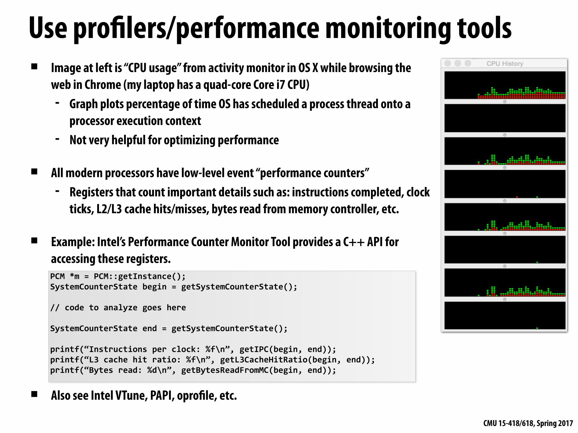
Use profilers/performance monitoring tools▪ Image at left is “CPU usage” from activity monitor in OS X while browsing the

web in Chrome (my laptop has a quad-core Core i7 CPU) - Graph plots percentage of time OS has scheduled a process thread onto a

processor execution context - Not very helpful for optimizing performance

▪ All modern processors have low-level event “performance counters” - Registers that count important details such as: instructions completed, clock

ticks, L2/L3 cache hits/misses, bytes read from memory controller, etc.

▪ Example: Intel’s Performance Counter Monitor Tool provides a C++ API for accessing these registers.

▪ Also see Intel VTune, PAPI, oprofile, etc.

PCM*m=PCM::getInstance();SystemCounterStatebegin=getSystemCounterState();

//codetoanalyzegoeshere

SystemCounterStateend=getSystemCounterState();

printf(“Instructionsperclock:%f\n”,getIPC(begin,end));printf(“L3cachehitratio:%f\n”,getL3CacheHitRatio(begin,end));printf(“Bytesread:%d\n”,getBytesReadFromMC(begin,end));