lecture 9. heteronuclear 3d nmr spectroscopy.logan/teaching/bch5886/lecture_9.pdflecture 9....

Macromolecular NMR Spectroscopy BCH 5886T.M. Logan Spring, 2005

Lecture 9. Heteronuclear 3D NMR Spectroscopy.The isotope-editing experiments discussed in the last lecture provide the conceptual

framework for heteronuclear 3D NMR experiments. These experiments are the foundation for determining the high resolution structures of proteins, protein-drug complexes, nucleic acids, and nucleic acid - protein complexes studied in structural biology. Today, we’ll discuss some of the more commonly used double resonance 3D / 4D experiments. First, though, I’ll provide some motivation for the study and use of these pulse sequences.

9.1. Why 3D / 4D NMR Spectroscopy?As proteins (and nucleic acids; I’ll just refer to proteins in these lectures, but you can easily

substitute nucleic acids, or any compound) approach and pass ~ 10 kDa (10,000 amu for you chemists) in molecular weight, two this happen to the NMR spectra:

• They become more crowded due to the increasing number of 1Hs in the sample; this complicates chemical shift assignment by making even 2D spectra increasingly overlapped.

• As the molecules increase in size, they tumble more slowly, and sensitivity decreases due to more efficient T2 relaxation. This leads to a decrease in the amount of anti-phase magnetization (proportional to sin(πJt1)) that can be built up

during t1 evolution periods of 2D 1H-1H experiments, leading to poorer performance in these experiments.

3D and 4D heteronuclear NMR experiments overcome these problems because:

• overlap is minimized by spreading the resonances over 3 or 4 different frequency dimensions, as opposed to just 1 or 2. It is important to realize that the number of resonances (or cross peaks) in 2D spectra is not reduced in these experiments, but that the “density” of cross-peaks is diminished due to heteronuclear editing, and

• coherence transfer is accomplished, wherever possible, through larger scalar coupling constants. Because J is larger, anti-phase states build up more rapidly, and relaxation during t1 (or other delays) is minimized. For example, a three-bond 1H-1H coupling of ~ 7 Hz (between, say on 1Hs on adjacent carbons) takes about 70 ms to completely evolve an antiphase magnetization (1/2J). However, developing the same correlation by evolving 1H-13C (1JCH = 151 Hz), then 13C-13C 1JCC = 35 Hz), and 1H-13C couplings, takes only about 21 ms (see Figure 9.1). Therefore, these experiments can regain many of the sensitivity losses incurred.

Of course, there are additional complications that arise by using heteronuclear experiments, but we’ll save our discussion of them until later in the lecture. Schematically, 3D and 4D experiments can be considered as consisting of sequential “2D’ building blocks, each of which consists of preparation, evolution, and mixing periods (see Figure 7.1). By concatenating

1


different 2D building blocks together, we generally drop the intervening relaxation and (t2) acquisition periods so that they occur only once, at the beginning and end of each sequence, respectively, just as we did for the isotope editing / filtering sequences.

9.2. Converting the Isotope-Edited 2D NOESY into a 3D Sequence; The NOESY-HMQC.

Recall the 2D isotope-edited 1H-1H NOESY sequence, shown in Figure 9.2a. As discussed in Lecture 7, this sequence consists of a 2D NOESY sequence building block (consisting of preparation, evolution, and mix / read periods) that is combined with a heteronuclear-editing spin echo building block (also with these periods; note that the “read pulse” of the NOESY building block is the first pulse of the “preparation” period of the HMQC). In this sequence, all 1Hs are evolving during the t1 period (all 1Hs means those that are bound to 15N, say, and those that are

not), and all 1Hs are exchanging magnetization through dipolar interactions during τm, but

immediately before detection, we remove 1Hs that are not scalar coupled to 15N (recall that this takes two scans). As shown in the notes for Lecture 7, this results in a 2D NOESY spectrum consisting of diagonal and cross peaks. However, the only diagonal peaks detected are in the amide 1H region of the NMR spectrum (see Figure 7.22 to refresh your memory).

Now consider the pulse sequence shown in Figure 9.2b. This is essentially the same pulse sequence of part A, but it has been modified to allow for chemical shift evolution of 15N during the

H

C C

HH

C C

H

3JHH ~ 7 Hz1JCH = 151 Hz1JCC = 35 HzFigure 9.1.

70 ms3.3 ms

14.3 ms

3.3 ms

τmt1 τ τ

decouple

+,-

0,180

d1A. 1H

15N

τmt1 τ τ

decouple

d1B. 1H

15Nt2

relax evol 1 mix 1 prep 2 evol 2mix /

acquireprep 1

read 2read 1

Figure 9.2. A. 2D Isotope filtered NOE sequence. B. Converting this sequence to 3D Noesy-HMQC sequenge. In both cases τ = 1/2J.

2


t2 time period using an HMQC building block. If we set t2 = 0, we get a 2D spectrum; the data obtained is exactly equivalent to that obtained using sequence 9.2a. What happens as we systematically increment the value of t2? Using a product operator analysis, we can easily show that the part of the sequence after τm gives a term that looks like -IxNz after the first τ period (see the notes from Lecture 7 on the HMQC pulse sequence), modulated by some sort of term that indicates chemical shift during t1 and any NOE magnetization transfer that occurred during τm. Applying the first 90° pulse on the N spin generates multiple quantum terms (see Eqn 7.11) that evolve under chemical shift during t2; the second 15N 90°x pulse reconverts this into 1H-15N antiphase magnetization that is refocused during the second τ period. Therefore, at the beginning of the acquisition period, we have terms that look like (the

exact form is slightly more complicated (see Eqn 7.13). These terms evolve under 1H chemical shift and 1H-1H scalar coupling during t3 (1H-15N scalar coupling is eliminated by 15N decoupling) to give a signal that is a function of three different time domains:

. [7.1]

The signal has been frequency-labeled twice; with a 1H frequency during t1 and an 15N frequency during t2. Fourier transforming this three-dimensional data matrix provides another three-dimensional data matrix where the axes are frequency instead of time:

[7.2]

where ω1 = (all) 1H, ω2 = 15N, and ω3 = 1HN. This experiment was first reported in 1989 by two different groups; Zuiderweg & Fesik,

(1989. Biochemistry 28, 2387-2391) at Abbott Labs, and Ikura, Kay & Bax, (1989. J. Am. Chem. Soc. 111, 1515-1517) at the NIH. In both cases, this experiment was applied to 1H-15N spin pairs, but as we discussed previously, the HMQC is NOT the experiment of choice when correlating 1H-15N spins. Therefore, a better version of the NOESY-HMQC pulse sequence was developed that uses an HSQC-type building block to transfer coherence from 1H-15N and back, Figure 9.3. 13C-edited 3D experiments soon followed, retaining the HMQC mode for heteronuclear editing (Ikura, Kay & Bax. 1990. J. Magn. Reson. 86, 204-209).

In the next several sections we’ll discuss various “practical” aspects of these experiments in more detail.

Iy ΩHat1( ) ΩNt2( )coscos

S t1 t2 t3, ,( ) Iy ΩHat1( ) ΩNt2( ) ΩHbt3( )coscoscos∼

S t1 t2 t3, ,( ) S ω1 ω2 ω3, ,( )↔

τmt1 τ τ

decouple

d11H

15Nt2

τ τ

±y

The 3D 15N-separated NOESY-HSQC experiment

Figure 9.3.

3


9.3. Spectral Appearance and Analysis.The main purpose of these 3D heteronuclear experiments (besides keeping biomolecular

NMR people busy) is spectral simplification. This is shown schematically in Figure 9.4 and with real data in Figure 9.5. Figure 9.4 shows a schematic version of a 2D isotope-edited NOESY experiment, which corresponds to the first t2 increment of a 3D 15N-separated NOESY-HSQC

spectrum. As seen in the 2D, there are correlations between amide 1HN and other 1Hs, but the congestion in the amide 1H chemical shift range can lead to ambiguities in assignments (yes, that’s what that is supposed to show). On the other hand, by evolving (and Fourier transforming) the 15N chemical shift in the 3D spectrum, we can separate these individual amide resonances by the chemical shift of their attached 15N. The data consist of a three-dimensional “cube” of frequency points; correlations between spins are indicated as “intensity” just as in 2D and 1D spectra. However, the data are not analyzed in cubes; rather the 2D planes at each 15N chemical shift are drawn on a computer, and you move through the 15N chemical shift dimension by drawing the appropriate plane (see Figure 9.5). The best analogy that I can come up with is that of using transparencies - each 2D transparency contains information that can be analyzed by someone. If all of these 2D transparencies are stacked one on top of another to form a 3D cube the information is still there but it is more difficult to see or to easily discern one slide from the adjacent ones. Obviously it is much simpler to present each 2D transparency as a single slide rather than as a 3D cube of slides.

Like a 2D spectrum the 3D spectrum consists of “diagonal” and “cross” peaks, which now have slightly different meanings. In 3D spectra, a diagonal peak is one in which the (1H) chemical shift in ω1 and ω3 are equal (e.g., they are the same 1HN resonance in the examples discussed here). A 3D cross peak has ω1 ≠ ω3. Of course, there can be no case in these heteronuclear

..

. . .. . ...... . ......

.. .. ... .H

H

w3 = HN

w1 = H

w2 = N

2D

3D

Figure 9.4. Schematic depiction of how 3 frequency dimensions reduces signal overlap in 2 frequency dimensions. The idea is analogous to the simplification of 1D spectra by 2D spectra.

4


spectra where ω1 = ω2 = ω3. Note that there are no additional resonances in this 3D spectrum than in the corresponding 2D spectrum, they are simply filtered and spread out over additional frequency space.

9.4. Phase Cycling and Experiment Time.Just as a 2D spectrum consists of a series of 1D spectra collected at different t1 delay times,

a 3D spectrum is a series of 2D spectra collected as a function of incrementing the t2 delay time. Generally, 40 - 64 t2 points are collected to get the desired resolution in the X nucleus chemical

10.0 9.0 8.0 7.0 10.0 9.0 8.0 7.010.0 9.0 8.0 7.0

0

1

2

3

4

5

6

7

8

9

10

15N = 113.2 ppm, ω2 15N = 123.315N = 117.0

Figure 9.5. Three 2D planes from a 3D 15N-separated NOESY-HSQC experiment performed on FKBP. The chemical shifts of the 15N dimension are indicated. Diagonal peaks are indicated by the solid line.

1H, ppm ω3

1H, ω2

5


shift; this places strict limits on the number of t1 points, and the total number of scans per FID. This is because 1. NMR people are inherently impatient (often this trait is coupled with an extremely short attention span), and 2. NMR magnets need to be filled periodically with liquid N2 and He to maintain the superconductivity of the magnet. The N2 fills occur every 10 days or so, and this places a real physical limit to any 3D sequence that is being run. Let’s take a second look at the NOESY-HSQC pulse sequence, reproduced in Figure 9.6. The difference between this Figure and 9.3 is the addition of a phase cycle. There are a few general guidelines followed in developing the phase cycle for 3D / 4D experiments. 1. keep it short, 2. shorten it again (generally never more than 8 scans / FID), 3. do axial peak suppression in every dimension. 4. use separate steps for each individual phase cycle, and 5. if time permits, add an additional phase cycle to cancel natural polarization of the heteronucleus in the INEPT / HSQC building block. Recall that axial peak suppression requires a two-step phase cycle, x,-x with the receiver cycled as x, -x, to be applied to the 90° pulse that starts an incrementable evolution delay (Note that in the following 0 = x, 1 = y, 2 = -x, and 3 = -y). Following guideline 3, we would set φ1 =02 and φ3 =02. However, guideline 4 says that two phase cycles should not run simultaneously so we set φ1 = 0202 and φ3 = 0022. The receiver phase is simply the sum of these two phase cycles; 0220. Here the sum is calculated using “modulo” math, where the idea is to divide any number by the “modulus” (in the case of NMR the modulus is 4 because we have four phases corresponding to x, y, -x, and -y)), and write in the remainder. A phase of 0 gives 0 (written as mod4(0) = 0); mod4(2) = 2; mod4(4) = 0; mod4(6) = 2, and etc.

We now have a four-step phase cycle and we can generally work with an 8-step in most 3D experiments; let’s add in a phase cycle that will cancel the natural polarization of the 15N spins in the INEPT. Recall that this requires φ2 to cycle as 1,3 and the receiver to cycle as 0,2 (see Lecture 5 if this is unfamiliar to you). To accommodate guideline 4, we set φ2 = 1111 3333, and change the receiver to 0220 2002. This is outlined in Table 9.1. Note that it is largely arbitrary whether φ1, φ2, or φ3 is set to a 2, 4, or 8-step phase cycle. The key is to cover all the necessary

τmt1 τ τ

decouple

d11H

15Nt2

τ τ

φ2φ1

φ3

Figure 9.6. 3D 15N-separated NOESY-HSQC sequence. Note that this sequence is now typically run using sensitivity enhancement and gradient coherence selection, as outlined in lecture 8.

6


phase cycles.

The phase cycle described here results in 8 steps / FID. But we haven’t yet discussed how we will generate phase discrimination of the frequencies oscillating in either t1 or t2, i.e., how do we add the hypercomplex phase cycles needed? If we were to run the experiment as a 2D, evolving t1, say, but not t2, then we would increment the phase of φ1 and the receiver by 90° on every second FID, such that 2 FIDs (of 8 scans each) are collected per t1 time period (see lecture 7, section 7.3) to generate the absorptive and dispersive components of the signal. If we were to evolve the 15N chemical shift in a 2D experiment, we would increment the phase of φ3 and the receiver instead. To run a 3D, we need to do both. Therefore, for each t1 time point, two “orthogonal” FIDs are collected (incrementing φ1 and receiver), for each t2 time point, two “orthogonal” 2Ds are collected (inrementing φ3 and receiver). The way to think about this is nested looping in computer program (because that’s exactly how these experiments are programmed). A schematic of the experiment in pseudo-computer code is presented in Figure 96.

What is the time commitment to running one of these experiments? There is a small bit of set-up time for the NOESY-HSQC that consists of calibrating 1H and 15N 90° pulses, and then deciding your spectral sweep widths and desired digital resolution (see below). Typically, one runs about 96 or 128 complex t1 increments (that is, two FIDs / increment), resulting in a 2D spectrum every 40 - 60 minutes. In addition, it si common to run about 40-48 complex t2 time points, which means anywhere between 80-96 hours (3 - days) for a normal 3D 15N-separated NOESY-HSQC experiment. The spectra shown in this chapter were collected using this type of acquisition. However, not all 3D experiments require this amount of time. As we’ll see later, there are experiments that can be run in as little as 18-24 hours. In summary, the limitations in determining the duration of a 3D sequence are 1. covering the minimal phase cycle, 2. collecting adequate digital resolution (not too many or too few points), and, 3. more practically, how much

Table 1: Minimal Phase Cycle for 3D NOESY-HSQC Experiment.

scan φ1 f2 φ3 rcvr

1 0 1 0 0

2 2 1 0 2

3 0 1 2 2

4 2 1 2 0

5 0 3 0 2

6 2 3 0 0

7 0 3 2 0

8 2 3 2 2

7


time is left in your turn on the spectrometer.Gradient coherence selection in the HSQC portion of these sequences can shorten the

phase cycle and is routinely incorporated into these sequences, as is the sensitivity enhancement process that we discussed in Lecture 8. Still, this does not significantly shorten the duration of these experiments.

9.5. Digital Resolution and Processing in 3D Spectra.I’ve made a few comments on digital resolution. Let me make a couple more for clarification.

Digital resolution is defined simply as the ratio of the sweep width to the number of points used to digitize (or represent) the spectrum. For example, on a 500 MHz NMR, I generally use an observed (t3) sweep width of 8333 Hz, and digitize it with 512 - 1024 complex points for a digital resolution of 16 or 8 Hz / pt. I’ll often use 96 complex t1 increments to digitize ~ 6250 Hz sweep

width in the indirect 1H dimension, and 48 complex points to cover 1650 Hz in the 15N dimension. This results in digital resolutions of 65, 34, and 16 Hz / pt in t1, t2, and t3, respectively. This has a

few practical considerations. 1. 1H-1H couplings are generally NOT resolved in 3D spectra, 2. natural 1H and 15N linewidths are often less than this, leading to truncation artifacts in the Fourier transform, and 3. some sort of resolution-enhancement is needed in processing. Finally, the collected data set size for a 3D similar to the one I just described is 1024 x 192 x 96 x 4 = 75.5 MBytes. Often, one can discard the data outside of the 1H amide region in the t3 dimension (there are no peaks there because we’ve filtered them out), so the raw data size is ~ 37 MBytes. However, during processing, it is common to increase digital resolution to 24, 12, and 8 Hz / pt, resulting in a final data set size of ~ 134 MBytes.

Processing of 3D data sets is performed analogous to 2D spectra. The data along the t3 domain (the rows) of the first 2D are Fourier transformed first to provide a first look at the data which allows you to make some judgements about the overall quality of the spectrum. The second FT is performed on the columns of the same 2D, resulting in the first 2D plane of the 3D being completed transformed to the frequency domain. Again, similar to the 2D case, where the

start sequence;set 1H, 15N increment counters = 0;

for t2 < t2, max,set φ3, rcvr = initial values;for t1 < t1,max,

set φ1, rcvr = initial values;collect 8 scans for complete phase cycle;write to disk;increment φ1, rcvr by 90°;

increment t1;increment φ3, rcvr by 90°;

increment t2;end;

Figure 9.7. Outline of phase cycle and increment looping in a typical 3D experiment. This scheme has the t1 dimension looping faster than the t2 loop. Alternatively, the t2 increment and phase can be the inner loop. The end result is the same.

8


first 1D looks like a normal 1D, this first 2D looks like a “normal” 2D, except that each of the peaks in the 2D have been frequency-labeled by an 15N chemical shift. The FT in the third dimension (the tubes) is performed analogous to the previous 2 FTs. It should be mentioned that the order of the FTs doesn’t matter and quite complicated processing schemes can be developed that involve FT, linear prediction to extend the data in some time domain, reverse FTs, and etc. Linear prediction is a mathematical extension of the collected data; the oscillations can be represented as a time-series of cos and sin terms with weighting coefficients. In linear prediction, the coefficients for the next “n” points are calculated based on the values of the previous “p” points. For short extensions, the fidelity of this process is very high; for long extensions, the fidelity drops.

9.6. Isotope Incorporation.The key to these heteronuclear experiments is to have uniform isotope enrichment at levels

approaching 100%. This is not as difficult as it sounds since most proteins are produced by recombinant methods. The idea is to grow the bacteria containing the expression vector in a defined (minimal) growth medium (called M9), where all of the 15N (and / or 13C) sources are labeled in 15N (or 13C). The most common approach is to grow the bacteria in M9 medium, which is essentially phosphate buffer, pH 7, with 5 g / L NaCl for osmotic pressure. The sole carbon and nitrogen sources are 15NH4Cl and U-13C6-glucose, at 1 and 2-4 g / L, respectively. In the old days (when I was a post-doc) this was very expensive as the NH4Cl cost ~ $60 / g, and the glucose cost ~ $600 / g. These days, however, the costs have decreased significantly (to about $25 and $150, respectively) so production of isotope-labeled proteins is not as limiting as it once was (you still spend a fair amount of time optimizing growth, expression, and purification conditions prior to producing labeled protein, though). A thorough review of this labeling process can be found in Muchmore et al (1989) Methods Enzymol. 177, 44-73. More recent “tricks” applied to labeling can be found in Marley et al. (2001) J. Biomol. NMR 20, 70-75. Here, the objective is minimize the labeling costs even further by growing the bacteria to normal density in “rich” medium, then spinning the cells down and resuspending them in a minimal amount of isotopically enriched M9 medium (~ 250 mL) where protein expression is induced.

9.7. Other Important Double-Resonance 3D Experiments.15N-separated Experiments. The most important of these experiments are the 15N-

separated TOCSY-HSQC, NOESY-HSQC and ROESY-HSQC experiments. The most commonly used versions of these first two sequences were developed by Lewis Kay at University of Toronto

t1 t t

decouple

d1

t2

t t

φ2

spin-lock

φ1

φ3

Figure 9.8.

9


(Zhang et al, 1994 J. Biomol. NMR 4, 845-858) and the 3D HNHB (Archer et al 1991 J. Magn. Reson. 95, 636-641 and Bax et al (1994) Methods Enzymol. 239, 79-105). The sequences for the TOCSY- and ROESY-HSQC experiments are shown in Figure 9.8 (with the sensitivity enhancement and gradient coherence selection are not shown for simplicity). The sequence for the HNHB is not shown. The phase cycle is the same as that discussed above for the NOESY-HSQC experiment (see Table 9.1), and the major difference between the TOCSY-HSQC and ROESY-HSQC is the nature of the spin locking pulse (see Lecture 7). The data from the TOCSY-HSQC (Figure 9.9) are used to identify intra-residue HN-Hα and HN-Hβ correlations, and is

0

1

2

3

4

5

6

7

8

9

10

10.0 9.0 8.0 7.0 10.0 9.0 8.0 7.010.0 9.0 8.0 7.0

15N = 113.2 ppm 15N = 123.315N = 117.0

Figure 9.9. Three 2D planes from a 3D 15N-separated TOCSY-HSQC experiment performed on FKBP. The chemical shifts of the 15N dimension are indicated and correspond to the same planes shown in Figure 9.5. Diagonal peaks are indicated by the solid line. Note that many fewer amide-sidechain correlations are observed in this spectrum compared to what was shown in Figure 7.19 and 7.20. The spinlock pulse is typically applied for shorter durations in the 3D sequence because the larger proteins relax more efficiently, limiting the extent of coherence transfer.

1H (ω3), ppm

1H (ω2)

10


always analyzed in conjunction with the NOESY-HSQC experiment. Three 2D planes from a TOCSY-HSQC experiment run on FKBP are presented in Figure 9.9. These planes are at the same 15N chemical shift as those from the NOESY shown in Figure 9.5. The data are analyzed by displaying the same 15N chemical shift (2D plane), and finding the corresponding diagonal peaks in the TOCSY and NOESY spectra. The HNHB experiment provides correlations between HN and Hβ of amino acid sidechains. This is a relatively insensitive experiment and is not always used but can be very helpful in certain circumstances.

13C-separated Experiments. There are two classes of common double-resonance 3D 1H-13C experiments: the 13C-separated NOESY, and the HCCH-TOCSY experiments. The former is used in structure determination, the latter in chemical shift assignment. We’ll discuss the NOESY experiment first and then the HCCH-TOCSY.

As discussed previously, the experiment of choice for making 1H-13C correlations is the HMQC, and this type of correlation is used in the 3D 13C-separated HMQC-NOESY experiment, shown in Figure 9.9. The minimal phase cycle consists of axial peak suppression on φ1 and φ2, and φ3 cycled as 02, or in a complete CYCLOPS phase cycle, resulting in either an 8-step or 16-step phase cycle. There are three comments to make here.

First, the isotope editing step comes first in this sequence (compared to the NOESY-HSQC experiment). This means that the 13C chemical shift separation is provided on the 1H from which the NOE originates (in the 15N experiment, we edit the destination 1H). The scheme used in this experiment provides the highest digital resolution on the detected NOE in the 13C-edited data. It also allows us to provide more stringent solvent suppression methods during the NOESY mixing time than can be applied during the 13C evolution time.

Second, the 13C-13CO scalar coupling is about 55 Hz (compared to ~ 35 Hz for 1JCC). Therefore, CO decoupling is generally performed during t2 using a relatively low-power 180° pulse to minimize excitation of the other carbons; this pulse is generated as a shaped-selective pulse (see Lecture 4).

Third, the number of 13C points in t2 is limited to approximately 1 point / ppm. This is

because of the size of the 1JCC and the need to minimize the evolution of this coupling. Evolving

the 13C chemical shift in t2 long enough to develop significant 13C-13C scalar coupling would dramatically decrease the sensitivity of the experiment (because the resonances would be split over the entire 13C multiplet). So how long is the acquisition time in t2? The 13C-13C couplings

τmτ τ

decouple

d11H

13Ct2

t1

φ1

φ2

φ3Figure 9.10.

11


develop as sin(πJt2), and we would like to keep this term to about 50% maximal value to optimize resolution and sensitivity (~40° angle; take my word for it). This limits us to about 7 ms of t2

acquisition time. For experiments on a 500 MHz (1H) spectrometer, 13C sweep width of about 70 ppm gives about 8800 Hz sweep width, and a dwell time of ~ 114 µs; the number of points is obtained from t2 acquisition time divided by t2 dwell time ~ 62 points, or roughly 1 point / ppm. Note that more points can be collected when using the 900, for instance, because the larger 13C bandwidth results in shorter dwell widths. Nevertheless, you still want to limit the 13C acquisition to ~ 7 ms.

The HCCH-TOCSY Experiment. The HCCH-TOCSY experiment was developed to provide sidechain 1H-1H correlations for purposes of chemical shift assignment (Kay, et al. 1990 J. Am. Chem. Soc. 112, 888-889; Bax et al. 1990 J. Magn. Reson. 88, 425-431). The idea is exactly as I described at the beginning of this lecture; coherence transfer through the large 1J scalar couplings provides efficient transfer, and gives strong cross peaks where direct transfer from 1H-1H would yield very poor transfer due to efficient relaxation. If you ask an experimental NMR spectroscopist which experiment is their least favorite, they are likely to say this one, not because of the experiment itself, which involves some nifty spin physics, but because the data are tedious to analyze. Unfortunately, there are few alternatives for obtaining the 1H sidechain assignments.

The pulse sequence is shown in Figure 9.11. The sequence consists of the following building blocks: a refocused-INEPT transfer from 1H to its attached 13C; 1H and 13C chemical shifts are encoded in the t1 and t2 evolution times, respectively. This generates carbon magnetization immediately prior to the TOCSY mixing sequence that is in-phase with-respect to its attached 1H (this requirement for in-phase magnetization precludes using the more-sensitive HMQC transfer). Carbon coherences are transferred during the TOCSY mixing scheme (generally people use the DIPSI-2 isotropic mixing sequence which is particularly adept at isotropic transfer over the large bandwidths encountered in carbon-carbon TOCSY), and the 13C magnetization is then transferred to its attached 1H via a reverse, refocused-INEPT sequence. 1H magnetization is detected during the t3 period.

A qualitative product operator analysis yields the following. Immediately after the φ1 1H 90°

pulse, we have -Iy that evolves under 1H-13C scalar coupling during 2τ1 (τ1 = 1/4J) to provide

δ δ δ δd1 t1τ1 τ1 τ2

τ2

2t12

t22

t22 decoupleDIPSI-2

The HCCH-TOCSY Pulse Sequence

φ1 φ2

φ3

Figure 9.11.

12


IxSz magnetization prior to the φ2 1H pulse. Following the simultaneous 1H-13C 90° pulses, we

have terms proportional to IzSy, which evolves under 1H-13C scalar coupling to give IzSy → Sx.

During the isotropic mixing sequence, 13C magnetization on spin 1 is transferred to spin 2, and we end up with the overall transfer S1x → S2x, which evolves again under 1H-13C scalar couplings during the first 2δ period to give terms proportional to IzSy. The two simultaneous 90°s

and the subsequent 2δ period serves to refocus the anti-phase 1H-13C term (IySz → Ix) for detection.

A few comments on the HCCH-TOCSY experiment.1. The t1 evolution and 1H → 13C INEPT sequences are combined to save time in the

experiment. Of course, the time we are interested in is beating relaxation of either 1H or 13C, so saving a few milliseconds can pay off. This combination is shown in more detail in Figure 9.12. As seen in the Figure, the combination method is quite similar to the traditional method for accomplishing both 1H frequency labeling and polarization transfer, except that we’ve eliminated one 13C 180° pulse. That these two methods give both chemical shift only during t1 and polarization transfer only during the 2τ period can be determined from the following. Using the traditional way, we would use product operators to say that chemical shift is operative of all of t1, but the “positive” sense of precession in the first τ period is cancelled by a “negative” sense precession in the second τ period (we could cancel all chemical shift evolution by extending the second τ delay to equal τ + t1). Considering just the sign of the product operator terms, we would say that the traditional method, chemical shift precesses as

[7.3]

Scalar coupling, on the other hand would go as

[7.4]

Note that the chemical shift term is not affected by the 15N 180° pulse where as the scalar coupling term is.

Now, look at the combination approach. Using the same approach of analyzing the signs of the product operator terms, we see that chemical shifts and scalar coupling are now active during

[7.5]

t1 τ τ t1τ τ

traditional way improved combination

Figure 9.12.

chemical shift t1 τ τ t1=–+=

scalar couplingt12-----

t12-----– τ τ 2τ=––=

chemical shift τ t1 τ t1=–+=

13


, [7.6]

just as the traditional way, but we’ve saved ourselves the problem of an additional 13C 180° pulse. This can be very important in some applications, like large proteins, or high-dielectric solvents (where pulse power is decreased). This concatenation approach, as it is called, is used extensively in multi-dimensional NMR spectra, and in the case where t1 = 0, it can trivially be shown to equal the traditional way for polarization transfer. For a discussion of these ideas, see the paper by Kay, Ikura and Bax titled “The design and optimzation of complex NMR Experiments” 1991 JMR 91, 84-92).

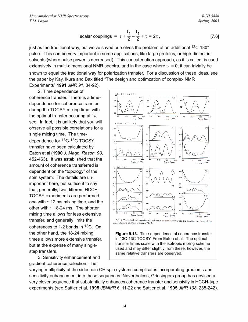
2. Time dependence of coherence transfer. There is a time-dependence for coherence transfer during the TOCSY mixing time, with the optimal transfer occuring at 1/J sec. In fact, it is unlikely that you will observe all possible correlations for a single mixing time. The time-dependence for 13C-13C TOCSY transfer have been calculated by Eaton et al (1990 J. Magn. Reson. 90, 452-463). It was established that the amount of coherence transferred is dependent on the “topology” of the spin system. The details are un-important here, but suffice it to say that, generally, two different HCCH-TOCSY experiments are performed, one with ~ 12 ms mixing time, and the other with ~ 18-24 ms. The shorter mixing time allows for less extensive transfer, and generally limits the coherences to 1-2 bonds in 13C. On the other hand, the 18-24 mixing times allows more extensive transfer, but at the expense of many single-step transfers.

3. Sensitivity enhancement and gradient coherence selection. The varying multiplicity of the sidechain CH spin systems complicates incorporating gradients and sensitivity enhancement into these sequences. Nevertheless, Griesingers group has devised a very clever sequence that substantially enhances coherence transfer and sensivity in HCCH-type experiments (see Sattler et al. 1995 JBNMR 6, 11-22 and Sattler et al. 1995 JMR 108, 235-242).

scalar couplings τt12-----

t12----- τ 2τ=+–+=

Figure 9.13. Time-dependence of coherence transfer in 13C-13C TOCSY. From Eaton et al. The optimal transfer times scale with the isotropic mixing scheme used and may differ slightly from these; however, the same relative transfers are observed.

14


I have used this sequence and it really helps with proteins; I imagine it will work even better with RNA.

I’ll close this section with some spectra from an HCCH-TOCSY experiment (18 ms mixing time) collected on FKBP. Figure 9.14 shows an entire 2D plane from an HCCH-TOCSY experiment taken at the 13C chemical shift of 57.3 ppm (this is the Cα carbon region). We see diagonal peaks and cross peaks, with the cross peaks extending along ω3 from about 0 to 6 ppm, but the resonances in ω1

being limited to a more narrow 1H chemical shift range because the 13C chemical shift (of 57.3 ppm) limits you to protons on Cα carbons. Correlations then, are observed in this chemical shift range between Hα and other sidechain 1Hs. To see the Hβ, for instance, we would need to be in the Cβ region of the 3D spectrum.

In other words, to identify the 1H and 13C resonances for the entire aliphatic portion of an amino acid sidechain requires several different 2D planes. This is shown for a single amino acid, a valine in FKBP in Figure 9.15, which shows different “strips” taken from 2D HCCH-TOCSY planes drawn at different 13C chemical shifts. The chemical shift assignments for this amino acid are obtained by starting from Cα/Hα chemical shifts (we’ll discuss where these come from momentarily), and observing the 1Hs that are correlated with that Cα/Hα spin pair. In this example,

026 4

0

2

4

6

w3, 1H

w1, 1H

w2 13C 57.3 ppm

Figure 9.14. 2D plane from an HCCH TOCSY experiment showing correlations from the Hα to aliphatic sidechain protons of FKBP.

13C = 57.6 ppm

13C = 35.2 ppm

13C = 19.7 ppm

13C = 21.8 ppm

Ha

Hb

Hg1

Hg2

16 5 4 3 2

Figure 9.15. Combined slices of 3D HCCH showing a valine spin system

15


the Hα/Cα diagonal peak occurs at 5.95 / 57.6 ppm (in 1H and 13C, respectively), and 1H-1H correlations are observed at cross-peak frequencies of 2.58, 1.43 and 1.04 ppm, but we don’t know the 13C chemical shifts for the cross peaks. These are found by searching for the “symmetrical” peaks (e.g., the symmetry-related cross peak for the Hβ resonance detected on Hα/Cα is the Hα resonance detected on Hβ/Cβ) until the best match is found. This process is repeated until all the 1H and 13C resonances are obtained for each individual amino acid. The alignment of the resonances is quite good, and symmetry-related resonances should be found for every resonance in the spin system. To aid in the interpretation of this spectrum, I indicated the diagonal resonances (solid lines) and alignment (dotted lines) in different planes.

9.8. Triple-Resonance 3D NMR Experiments.These are the final major group, or class, of NMR experiments to be introduced in the

course. They are an extremely powerful group of experiments that are designed for purposes of chemical shift assignment in proteins and nucleic acids of size larger than 10 kDa. The idea for most of these methods is sketched in Figure 9.16, which shows a typical polypeptide backbone. In double resonance experiments, we develop 1H-1H correlations that are separated either by their attached 15N or 13C nucleus. In triple resonance experiments, we will generate correlations between 1H, 13C, and 15N resonances, and in virtually all cases, we will set up our experiments to detect a signal on an amide 15N and 1H because of the high chemical shift dispersion in 15N, its narrow line-shape (and long T2 relaxation times), and the high sensitivity of 1H. In a typical

triple resonance 3D experiment (3R3D), we may correlate the HN, N, and Cα of one amino acid. Another popular 3R3D experiment is to correlate HN,N, and CO; Hα,Cα and N; Hα,Cα, and CO, etc. (OK, so I realize that CO and Cα are the same nucleus if not atom but in this case we consider them to be 3R because we only detect one 1H frequency). We’ll examine a few of these in some detail in the next few sections. Finally, all sequences that correlate 1HN and 15N using an HSQC-type correlation contain sensitivity enhancement and gradient coherence selection, as outlined in Lecture 7. This is not explicitly shown in this lecture because it un-necessarily adds to complexity without introducing new concepts.

9.9. The HNCO and HNCA Experiments.One of the simplest and most sensitive 3R3D experiment is the HNCO (Ikura, Kay & Bax,

1990. Biochemistry 29, 4659-4667), which correlates HN, N, and CO, hence the name. The correlations are shown in Figure 9.16 in the circled nuclei , and the coherence transfer flow can

NN

O

O

O

H

HHR

HR

HN

N(Ω)

CO (Ω)

N

HNFigure 9.16.

16


be represented as shown in the right hand side of the figure: we start on 1HN, and transfer to their attached 15N using a refocused INEPT building block; the chemical shift of the 15N is measured. The 15N magnetization is transferred to CO, where chemical shift is measured, transferred back to 15N, and finally, back to 1HN (and measure chemical shift). The sequence is shown in Figure 9.17, and sample spectra are shown in Figure 9.18. We can dissect this experiment using product operators involving 1H, 15N, 13CO, and 13Cα spins (I,N,K, and S, respectively). At point a, we have evolved 1H magnetization in anti-phase with respect to its attached 15N, , which is converted in to antiphase 15N magnetization that evolves chemical

shift (but not 1H, 15N scalar couplings) during t1 to give terms proportional to at

point c (NOTE that we have decoupled 1H, 13CO and 13Cα during the 15N evolution period).The 15N terms are refocused with respect to 1H, and also evolve 15N-13CO couplings during the 2τ period (= 1/2JNCO; 1JNCO ~ 11 Hz) so that at point d we have terms given by

, which is converted into CO magnetization at point e. At point f, we have

encoded CO chemical shift, and re-converted the magnetization back to 15N, giving terms proportional to . This antiphase N magnetization is refocused with

respect to CO and dephased with respect to 1H, so that at point g, we have re-generated 1H magnetization in anti-phase with respect to its attached 15N. Immediately prior to detection we have terms proportional to . The sample spectrum on the left in Figure

9.16 represents a 2D version of the HNCO, with the spectra simplification afforded by evolving the 15N chemical shift indicated by the spectrum on the right.

Another very useful 3R3D experiment is the HNCA (Ikura, Kay & Bax, 1990. Biochemistry 29, 4659-4667), which is identical to the HNCO except that all CO pulses are executed on the CA nucleus, and vice-versa. The sequence is shown in Figure 9.17 (it is exactly the same pulse sequence as shown in Figure 9.15, but with the axis labels switched. The product operator analysis is the same, but in this experiment, we correlate HN, N, and Cα of each individual

IxNz

NyIz ωNt1( )cos

dect1

t2

δ δ δ δ

τ τ τ τ

H

N

CO

CA

The HNCO Experiment

a

b c d

e

f

g h

Figure 9.17.

NyKz ωNt1( )cos

NyKz ωNt1( ) ωCOt2( )coscos

Ix ωNt1( ) ωCOt2( )coscos

17


residue. However, the 1JNCα ~ 10 Hz, whereas the 3JNCα (to the Cα of the residue immediately preceding) is ~ 7 Hz. Since these values are similar, when we evolve under JNCα, we get correlations to the intra-residue Cα and the “i-1” Cα. This can sometimes be a nuisance, but can also be helpful in making assignments, as we’ll discuss in two weeks.

9.10. The HNCACB Experiment.A third, extremely important experiment is the HNCACB (Wittekind & Mueller. 1993 J. Magn.

15N (ω2) = 122 pm

Figure 9.18. A. 2D HNCO spectrum; B. single 2D plane taken at the indicated 15N chemical shift. Spectra were collected on the FKBP protein using standard pulse sequence.

ω2,

13 C

O, p

pm

ω3, 1HN, ppm

dect1

t2

δ δ δ δ

τ τ τ τ

H

N

CA

CC

The HNCA Experiment

a

b c d

e

f

g h

Figure 9.19.

18


Reson. 101B, 201-205; Muhandiram & Kay. 1994 J. Magn. Reson. 104B, 203-216), where you correlate Cα and Cβ frequencies with the intra-residue amide 1H and 15N. However, as in the HNCA, there often are correlations for Cα/Cβ of the preceding residue. I’ll show you the data, discuss its analysis, and then discuss the spin physics for this experiment.

The HNCACB experiment correlates the chemical shifts of four backbone resonances - HN, N, Cα and Cβ. In addition, as in the HNCA, correlations are obtained between the nitrogen of

dect2τ τ ττ

t1

δ δ δ δ

τcc τcc τcc τcc

δ2 δ2decouple

decouple

The HNCACB Experiment

H

N

Ca/Cb

CO

Figure 9.20.

70

60

50

40

30

20

11 10 9 8 71HN, ω3

13C, ω1

Figure 9.21. First 2D plane of a 3D HNCACB spectrum collected on the FKBP protein. The black resonances are phased positive and represent Cα carbons; the gray resonances are phased negative and arise from Cβ carbons. The gray lines are an artefact that results from the fact that Bill Gates doesn’t know how to implement Abode Illustrator on PC computers.

19


residue i and the Cα/Cβ of residues i and i-1. The data are analyzed in 2D planes with axes for 13C and 1HN chemical shifts in the 2D. Because of the way in which the experiment is performed, Cα and Cβ resonances are distinguished by a phase inversion of the Cβ. This is indicated in Figure 9.21 by the gray dots, which are negative. Notice in Figure 9.21 that although there is a general distinction in 13C chemical shift between the Cα and Cβ resonances, that there are many exceptions to this rule, so it is important to have this phase difference between them to help assign them. As shown in Figure 9.19, the data are analyzed by identifying intra-residue correlations (they are almost always more intense than the “sequential” correlations), identifying the “sequential” correlations, and finding the set of intra-residue correlations that align the best by scanning through the 15N dimension. The data show sequential strips taken from different 2Ds that indicate how the data are analyzed (Figure 9.22) . Notice in Figure 9.18 that although there is a general distinction in 13C chemical shift between the Cα and Cβ resonances, that there are many exceptions to this rule, so it is important to have this phase difference between them to help assign them. As shown in Figure 9.19, the data are analyzed by identifying intra-residue correlations (they are almost always more intense than the “sequential” correlations), identifying the “sequential” correlations, and finding the set of intra-residue correlations that align the best by scanning through the 15N dimension. The data shown are for residues F46-M49 of FKBP; the

NN

NN

O

O H

O H

O H

H

SH3C H3N

49Ca

49Cb

48Cb

48Ca

M49F48K47F46

Figure 9.22. “Strips” plot from HNCACB experiment indicating the sequential assignment information inherent in this experiment.

20

30

40

50

13C, ω1

20


correlations made are indicated in the Figure.The HNCACB pulse sequence is shown in Figure 9.20. The sequence starts on HN and

uses an INEPT sequence to transfer to nitrogen, and a second INEPT step to transfer from 15N to Cα. The relevant product operator term following the first INEPT transfer is which is

refocused with respect to 1H (to give after the δ2 delay) and dephased with respect to the

attached Ca scalar coupling constant so that after the first 2τ period we have where the Cα

product operator is given by . Immediately following the simultaneous nitrogen and carbon 90° pulses we generate transverse Cα magnetization in antiphase with respect to its attached nitrogen, , that evolves under 1JCC during the 2τcc period to give . The

carbon 90° y-pulse generates coherence transfer from Cα to Cβ to give terms

that are frequency labeled during t1. The carbon 90° -y-pulse at the end of t1 generates a second

coherence transfer from Cβ to Cα but leaves the Cα term unaffected, giving at the beginning of the second 2τcc period. During this

period the Cα-Cβ antiphase term is refocused (and selected by the phase cycle) giving two identical product operator terms that differ in phase (sign) and that are frequency labeled by different 13C chemical shifts:

.

This is the origin of the phase difference between the Cα and Cβ resonances.In the remainder of the sequence, the carbon-nitrogen antiphase terms are used to transfer coherence from Ca to nitrogen, and then on to 1H in the final INEPT step to give the final terms.

The HNCACB, HNCA, and HNCO triple resonance experiments are termed “out and back” experiments because the magnetization starts on amide proton (and nitrogen), is transferred out to other nuclei and than refocused back onto the amide proton at the end of the sequence. You might think that this approach is particularly silly, especially when faced with the substantial number of coherence transfer steps in the HNCACB. It would appear to be easier to start on the sidechain 1H, transfer magnetization to the attached 13C, then to Cα and then to amide nitrogen and proton, forming essentially a “straight-through” experiment. However, it turns out that there is one fundamental difference between these two sequences, and that lies in the amount of time in which the Ca magnetization is in the transverse plane. In the HNCACB experiment 13C is transverse for which translates into a maximum time of ~ 21 ms considering that

. For the CBCANH experiment, which was initially proposed by

Grzesiek and Bax (1992 JMR 99, 201-207), 13C magnetization is in the transverse plane for a total period of ( ).

Note that the optimal times for these delays begins to deviate from the delays chosen for simple two-spin H-N systems because the different multiplicity of the CH spin systems encountered in a protein require some sort of compromise time. Given an average 13Cα linewidth of ~ 15 Hz

IzNy

Nx

AzNy

A

AyNz– AyNz– NzAxBz+

AyNz– Nz– AzBy

AyNz ΩAt1( )cos– NzAxBz ΩBt1( )cos+

AyNz ΩAt1( )cos– NzAy ΩBt1( )cos+

4τcc t1+

2τcc 1 4Jcc( )⁄∼ 7 ms=

2τcc t1 2τcn+ + 7 ms 7 ms 22 ms+ + 36 ms= = 2τcn 1 4Jcc( )⁄∼ 22 ms=

21


corresponds to a T2 of ~ 21 ms (see Lecture 1 if you don’t recall how to make this conversion),

then we can see that carbon magnetization relaxes for approximately 1 x T2 (~ ) whereas the straight-through CBCANH experiment relaxes for ~ 1.7 x T2. This translates into ~ 36% and 19% of the original transverse magnetization surviving in each sequence, meaning that the HNCACB is rougly a factor of 2 more sensitive than the CBCANH.

The CBCA(CO)NH Experiment. The final triple-resonance experiment I will introduce in this lecture is the CBCA(CO)NH experiment (Figure 9.23), first introduced by Grzesiek and Bax (1992 JMR 99, 201-207) and modified for gradient coherence selection and sensitivity enhancement by Kay’s group (Muhandiram et al. (1994 JMR 103B, 203-216).

In this sequence, magnetization starts on the sidechain protons and is transfered to 13C using an INEPT transfer step. This generates product operators for both 13Cα and 13Cβ spins that evolve as and during the 2τcc period. The carbon 90° x-pulse at the end of the 2τcc

period has no effect on the but effects a transformation. During the ensuing

2τcco period Cα-CO scalar couplings are evolved and Cα - CO coherence transfer is effected by

the simultaneous 90° pulses prior to the 2τcon period. During the 2τcon period Cα-CO magnetization is refocused and carbonyl-nitrogen scalar couplings are evolved to generate

terms that are used to effect coherence transfer from carbonyl to nitrogen by the

simultaneous 90° pulses. After recording 15N chemical shift (during t2), refocusing the nitrogen-

carbonyl antiphase magnetization (during the 2τn period), and dephasing according to the 1H-15N scalar coupling (during the δ2 delay), nitrogen magnetization is transfered to 1H for detection via the final reverse INEPT sequence (if this makes any sense at all to you, take a moment to reflect on how much NMR you’ve learned!). In this sequence, unlike the HNCACB, the Cα and C correlations have identical phase. The data generated by this pulse sequence very much resembles the data obtained from the HNCACB experiment (Figures 9.21 & 9.22), but with only a single set of Cα/Cβ correlations per amide nitrogen / hydrogen, simplifying the analysis.

et T2⁄–

decτ

δ δ δ δ

τcc τcc

δ2decoupleH

N

Ca/Cb

CO

Figure 9.23. CBCA(CO)NH pulse sequence.

t12

-t22

τcco τcco

τt22

-t12

y

τcon τcon

Ax ByAz

Ax ByAz BzAy→

KyNz

22

lecture 9. heteronuclear 3d nmr spectroscopy.logan/teaching/bch5886/lecture_9.pdflecture 9....

Documents