lecture 8 - bone remodelling - university of sydney
TRANSCRIPT

The University of Sydney Page 1
Bone Remodelling
Andrian SueAMME4981/9981Week 9Semester 1, 2016
Lecture 8

The University of Sydney Page 2
Mechanical Responses of Bone
– Bone microstructure– Descriptions– Imaging
– Bone constitutive models and relationships– Stiffness and apparent density
– Bone remodelling mechanisms– Physiological responses to
mechanical stimuli– Models of bone responses
– Simple example calculations
Bodykinematics
Biomaterial mechanics
Biomaterial responses

The University of Sydney Page 3
Bone microstructureDescription and clinical imaging

The University of Sydney Page 4
Description of bone microstructure and composition
– Five major functions: load transfer; muscle attachment; joint formation; protection; hematopoiesis
– Composition and structure of bone heavily influences its mechanical properties– Collagen fibres– Bone mineral (hydroxyapatite)– Bone cells (osteoblasts, osteoclasts, osteocytes)
– Two classes of bone structure– Cancellous (or spongy) bone– Cortical (or compact) bone

The University of Sydney Page 5
Description of cortical bone microstructure
179CHAPTER 6 Skeletal System: Bones and Bone Tissue
of a fracture that heals improperly), the trabecular pattern realigns with the new lines of stress. Compact bone ( figure 6.6 ) is denser and has fewer spaces than cancellous bone. Blood vessels enter the substance of the bone itself, and the lamellae of compact bone are primarily oriented around those blood vessels. Vessels that run parallel to the long axis of the bone are contained within central, or haversian (ha-ver!shan), canals. Central canals are lined with endosteum and contain blood vessels, nerves, and loose connective tissue.
Concentric lamellae are circular layers of bone matrix that sur-round a common center, the central canal. An osteon (os!te-on), or haversian system, consists of a single central canal, its contents, and associated concentric lamellae and osteocytes. In cross section, an osteon resembles a circular target; the “bull’s-eye” of the target is the central canal, and 4–20 concentric lamellae form the rings. Osteocytes are located in lacunae between the lamellar rings, and canaliculi radiate between lacunae across the lamellae, producing the appearance of minute cracks across the rings of the target.
Interstitial lamellae
Periosteum
Blood vesselwithin a perforating(Volkmann’s) canalbetween osteons
Blood vesselswithin a perforating(Volkmann’s) canal
Blood vesselswithin a central(haversian) canal
Circumferentiallamellae
Concentriclamellae
Osteon (haversian system)
Blood vessel withinthe periosteum
Canaliculi
Osteocytes in lacunae
Canaliculi
Concentriclamellae
Lacunae
Central canal
LM 400x
FIGURE 6.6 Compact Bone(a) Compact bone consists mainly of osteons, which are concentric lamellae surrounding blood vessels within central canals. The outer surface of the bone is formed by circumferential lamellae, and bone between the osteons consists of interstitial lamellae. (b) Photomicrograph of an osteon.
(b)
(a)
see65576_ch06_173-202.indd 179see65576_ch06_173-202.indd 179 11/22/06 5:05:45 PM11/22/06 5:05:45 PM
CONFIRMING PAGES
The University of Sydney Page 6
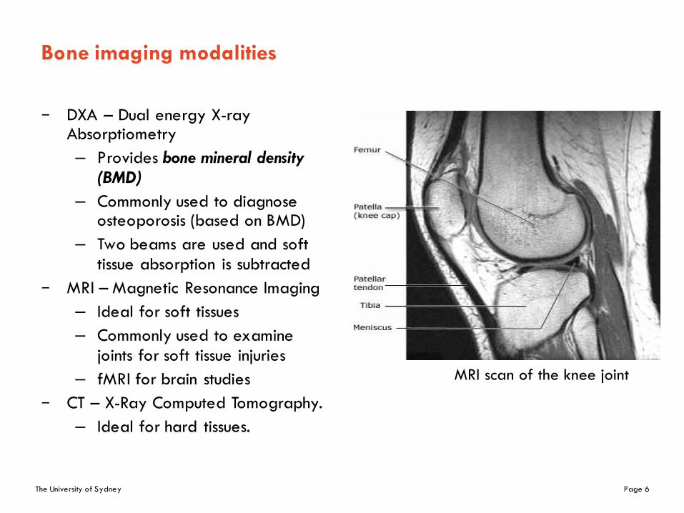
Bone imaging modalities
– DXA – Dual energy X-ray Absorptiometry– Provides bone mineral density
(BMD)– Commonly used to diagnose
osteoporosis (based on BMD)– Two beams are used and soft
tissue absorption is subtracted– MRI – Magnetic Resonance Imaging
– Ideal for soft tissues– Commonly used to examine
joints for soft tissue injuries– fMRI for brain studies
– CT – X-Ray Computed Tomography.– Ideal for hard tissues.
MRI scan of the knee joint

The University of Sydney Page 7
DXA – Dual Energy X-Ray Absorptiometry
GE Lunar DEXA Systems
354 CLEVELAND CL IN IC JOURNAL OF MEDICINE VOLUME 70 • NUMBER 4 APRIL 2003
and undergo treatment to prevent fractures.The only way to do this is to measure bone
mineral density. Low measurements on DXApredict the risk of fractures of the spine4 andhip,5 analogous to the relationship betweenhigh serum cholesterol and the risk of myocar-dial infarction, or between high blood pressureand the risk of stroke.6
Driving the demand for DXA is the avail-ability of proven, FDA-approved therapies forosteoporosis, ie, alendronate (Fosamax), rise-dronate (Actonel), calcitonin (Miacalcin),raloxifene (Evista),7 estrogen replacement ther-apy,8,9 and parathyroid hormone (Forteo).10
■ HOW DXA WORKS,HOW IT CAN GO WRONG
DXA uses x-rays at two energy levels to deter-mine the bone mineral content. This isaccomplished by subtracting the difference ofabsorption of x-rays between soft tissue and
calcium bone.The scanner software calculates the bone
mineral density, dividing the bone mineralcontent by the area of the region of interest.The bone mineral density is compared to ref-erence data specific to the scanner, and theresults are expressed as the T score and the Zscore (see below).
Although DXA could be used to measurebone density at many skeletal sites, two sitesare typically measured: the first four vertebraeof the lumbar spine posteroanteriorly, and theproximal femur (“hip”), including the femoralneck and the trochanteric areas and total hipmeasurement (FIGURE 1).
Opportunities for errorSeveral aspects of the bone density measure-ments should be evaluated before a study isaccepted as accurate.
Placement and sizing of the “regions ofinterest.” Changes in placement can signifi-
BONE DENSITOMETRY RICHMOND
DXA of the hip:Good scan “Problem” scans
FIGURE 1. Left, normal positioning for DXA of the hip. The lesser trochanter is minimally visualized or notvisualized, the diaphysis is parallel to the table edge. The hip is not abducted.Center, external rotation results in visualization of the lesser trochanter, shortening the femoral neck.The hip is also abducted. Improper positioning results in poor precision on follow-up studies because it isdifficult to reproduce the positioning. The exam data are also less reliable since the reference databasewas presumably collected with proper positioning.Right, loss of joint space from degenerative joint disease results in cortical thickening of the medial femoralneck region, falsely increasing bone mineral density measurement. Eccentric placement of the femoral neckregion of interest does not affect bone mineral density analysis. Reproducibility on subsequent scans is diffi-cult, especially as degenerative changes progress.
IMAGES COURTESY OF GE LUNAR MEDICAL SYSTEMS

The University of Sydney Page 8
Imaging of bone microstructure
– To examine the bone microstructure, high resolution scanning is required– Micro-CT and Nano-CT options have high resolution that allows visualisation
of bone microstructure
Imaging Modality Max. Resolution (in-vivo) in microns
Medical CT 200 x 200 x 200
3D-pQCT 165 x 165 x 165
MRI 150 x 150 x 150
Micro-MRI 40 x 40 x 40
Micro-CT 5 x 5 x 5
Nano-CT 0.05 x 0.05 x 0.05

The University of Sydney Page 9
Micro-CT of bone microstructure
– MicroCT Scanner (SkyScan 1172).– Micro-CT scan à sectional image
à segmentation à 3D image (STL)
– Limited field of view

The University of Sydney Page 10
Microstructural changes in cancellous bone
– Right: decreasing bone density with age as indicated.
– Bottom: comparison of bone density between a healthy 37-year-old male (L) and a 73-year-old osteoporotic female (R).
32-year-old male
59-year-old male
89-year-old male

The University of Sydney Page 11
Bone constitutive modelsStiffness and apparent density relationships

The University of Sydney Page 12
Power law relationship for cancellous bone stiffness
– Well-established relationship between apparent density (ρ) and cancellous bone Young’s modulus (E)
– a, p are empirically determined constants
𝐸 = 𝑎𝜌%
References p R2
Carter and Hayes (1977) J Bone Joint Surg Am, 59:954
3.00 0.74
Rice et al. (1988), J Biomech 21:155.
2.00 0.78
Hodgkinson and Currey (1992), J Mater Sci Mater Med 3:377
1.96 0.94
Kabel et al. (1999), Bone 24:115 1.93 0.94

The University of Sydney Page 13
Power law models for cancellous bone
– Hodgkinson – Currey model (1992)– Kabel isotropic model (1999)
– Yang (1999) – orthotropic cancellous model
φ – volume fraction and ρ – 1800φ kg/m3
𝐸&'() = 0.003715𝜌0.12
𝐸 = 𝐸34556' 813𝜑0.19 = 𝐸34556'813𝜌
1800
0.19= 𝐸34556'0.000424𝜌0.19
𝐸00 = 𝐸34556' 1240𝜑0.< , 𝐸>> = 𝐸34556' 885𝜑0.<1 , 𝐸99 = 𝐸34556' 529𝜑0.1>
𝐺>9 = 𝐸34556' 533.3𝜑>.AB , 𝐺09 = 𝐸34556' 633.3𝜑0.1D , 𝐺0> = 𝐸34556' 972.6𝜑0.1<
𝜈>9 = 0.256𝜑FA.A<2, 𝜈09 = 0.316𝜑FA.010, 𝜈0> = 0.176𝜑FA.>B<

The University of Sydney Page 14
Orthotropy of bone
– Material possesses symmetry about three orthogonal planes
– 9 independent components– 3 Young’s moduli:
𝐸0,𝐸>, 𝐸9– 3 Poisson’s ratios:
𝜈0> = 𝜈>0,𝜈>9 = 𝜈9>, 𝜈90 = 𝜈09– 3 shear moduli:
𝐺0>,𝐺>9,𝐺90
1
2
3
𝜖00𝜖>>𝜖992𝜖>92𝜖092𝜖0>
=
1𝐸0
−𝜈0>𝐸0
−𝜈09𝐸0
0 0 0
−𝜈0>𝐸>
1𝐸>
−𝜈>9𝐸>
0 0 0
−𝜈09𝐸9
−𝜈>9𝐸9
1𝐸9
0 0 0
0 0 01𝐺>9
0 0
0 0 0 01𝐺90
0
0 0 0 0 01𝐺0>
𝜎00𝜎>>𝜎99𝜎>9𝜎09𝜎0>

The University of Sydney Page 15
Orthotropic constitutive models of cortical bone
E3 (axial)
E2 (circumferential)
E1 (radial)
Young’s modulus Poisson’s ratio Shear modulus
E1=6.9GPa ν12=0.49, ν21=0.62 G12=2.41GPa
E2=8.5GPa ν13=0.12, ν31=0.32 G13=3.56GPa
E3=18.4GPa ν23=0.14, ν32=0.31 G23=4.91GPa
Young’s modulus Poisson’s ratio Shear modulus
E1=12.0GPa ν12=0.376, ν21=0.422 G12=4.53GPa
E2=13.4GPa ν13=0.222, ν31=0.371 G13=5.61GPa
E3=22.0GPa ν23=0.235, ν32=0.350 G23=6.23GPa
(Humpherey and Delange, An Introduction to Biomechanics, 2004)
Tibia
Femur

The University of Sydney Page 16
Homogenisation techniques for bone microstructure
Voxel-based FE model(element size: 25 microns)
– Directly transfer voxel to element (Grid mesh)
– Large number of elements– Stress concentration
Solid-based FE model(element size: 150 microns)
– Segmentation process– Smoothing, creation of geometry– Control of meshing algorithms
Perform static FEA under simple loading to determine the effective stiffness of these structures

The University of Sydney Page 17
Bone remodelling mechanismsPhysiological responses to mechanical stimuli

The University of Sydney Page 18
Concept of bone remodelling
– Living tissues are subject to remodelling/adaptation, where the properties change over time in response to various factors
– “every change in the function of bone is followed by certain definite changes in internal architecture and external conformation in accordance with mathematic laws.” – Julius Wolff (1892)
– Cancellous bone aligns itself with internal stress lines

The University of Sydney Page 19
Structural remodelling in bones
– Remodelling or adaptation can occur when there are changes in tissue environment, such as:– Stress/strain/strain energy
density– Loading frequency– Temperature– Formation of micro-cracks
– A good example is to look at the growth of trees around external structures– Thickening of branches near
fences/gates– Natural optimisation
Mattheck (1998)

The University of Sydney Page 20
Variations in bone remodelling responses
– Bone remodelling is thought to be mediated by osteocytes– Site dependency
– Different bones provide different mechanical function– Different sites have different biological environment– Results in different remodelling equilibrium
– Time dependency– High frequency (25 Hz) vs low frequency– Large load and low frequency can prevent mass loss– At higher frequencies, substantial bone growth is possible– Fading memory effects, i.e. adaptation of tissue to mechanical
stimulation

The University of Sydney Page 21
Mechanical signal transduction in bones
– Bone transduces mechanical strain to generate an adaptive response– Piezoelectric properties of
collagen– Fatigue micro-fracture
damage-repair– Hydrostatic pressure of
extracellular fluid influences on bone cell
– Hydrostatic pressure influences on solubility of mineral and collagenous component, e.g. change in solubility of hydroxyapatite
– Creation of streaming potential
– Direct response of cells to mechanical loading
These are all mechanisms which may allow mechanical strain to be detected by bone

The University of Sydney Page 22
Bone remodelling by micro-fracture repair
Increased stress causes cracks in
bone microstructure
Triggers osteoclast formation to
remove broken tissue
Osteoblasts are then recruited to help form new
bone
Osteoblasts become
osteocytes and maintain bone
structure

The University of Sydney Page 23
Bone remodelling by dynamic loading
– Dynamic loading is much more effective at stimulating bone growth.– Burr et al. (2002) found that dynamic loading forces fluids through canalicular
channels, stimulating osteocytes by increased shear stresses.

The University of Sydney Page 24
Models of bone responsesBone remodelling calculations

The University of Sydney Page 25
Mechanical stimuli - ψ
– Strain energy density
– Energy stress – linearise the quadratic nature of U
– Mechanical intensity scalar (volumetric shrinking/swelling)
– von Mises stress (σ1,σ2,σ3 – principal stresses)
– Daily stresses (ni = number of cycles of load case i, N = number of different load cases, m = exponent weighting impact of load cycles)
𝜓 = 𝑈 =12 𝜎 L 𝜀 =
12 [𝜎00𝜀00 + 𝜎>>𝜀>> + 𝜎99𝜀99 + 𝜎0>𝜀0> + 𝜎09𝜀09 + 𝜎>9𝜀>9]
𝜓 = 𝜎')'QRS = 2𝐸(TR𝑈
𝜓 = 𝜗 = 𝑠𝑖𝑔𝑛(𝜀00 + 𝜀>> + 𝜀99) 𝑈
𝜓 = 𝜎T& =12
𝜎0 − 𝜎> > + 𝜎> − 𝜎9 > + 𝜎9 − 𝜎0 >
𝜓 = 𝜎\ = ]𝑛4𝜎4&_
4`0
0&

The University of Sydney Page 26
Continuum model of bone remodelling
– Surface remodelling – changes in external geometry of bone (cortical surface) over time, e.g. radius of bone
Ψ(t) – Mechanical stimulus. It may also change with time.Ψ*(t) – Reference stimulus
– Internal remodelling – changes in a material property over time, e.g. apparent density
𝑆 = [𝑆 𝑡 ] 𝐶 = [𝐶 𝑡 ]

The University of Sydney Page 27
Surface remodelling
– Stimulus Error: deviation of stimulus from some baseline/ref. value.
– Surface Remodelling Rate: cs is a given constant.
– Surface Remodelling Rule with Lazy Zone: ws defines the lazy zone.
𝑒 = 𝜓 𝑡 − 𝜓∗(𝑡)
𝑑𝑠𝑑𝑡 = �� = 𝑐5 𝜓 𝑡 − 𝜓∗ 𝑡 = 𝑐5𝑒
�� = i𝑐5 𝜓 𝑡 − 𝜓∗ 𝑡 −𝑤5
0𝑐5[𝜓 𝑡 − 𝜓∗ 𝑡 +𝑤5]
for𝜓 𝑡 − 𝜓∗ 𝑡 > 𝑤5for − 𝑤5 < 𝜓 𝑡 −𝜓∗ 𝑡 < 𝑤5
for𝜓 𝑡 − 𝜓∗ 𝑡 < −𝑤5

The University of Sydney Page 28
The lazy zone model for surface remodelling
Alternative remodelling rule without lazy zone:
�� = i𝑐5 𝜓 𝑡 − 𝜓∗ 𝑡 −𝑤5
0𝑐5[𝜓 𝑡 − 𝜓∗ 𝑡 +𝑤5]
�� = 𝑐5[𝜓 𝑡 − 𝜓∗ 𝑡 ]
�� = 𝑐5𝜓 𝑡 − 𝜓∗ 𝑡
𝜓∗ 𝑡
Surf
ace
rem
odel
ling
rate
(Ṡ)
Mechanicalstimulus (ψ)
ψ*
Lazy zone
ψ*–w
s ψ*+w
s

The University of Sydney Page 29
The lazy zone model for internal remodelling
Alternative remodelling rule without lazy zone:
�� = i𝑐q 𝜓 𝑡 − 𝜓∗ 𝑡 −𝑤5
0𝑐q[𝜓 𝑡 − 𝜓∗ 𝑡 +𝑤5]
�� = 𝑐q[𝜓 𝑡 − 𝜓∗ 𝑡 ]
�� = 𝑐q𝜓 𝑡 − 𝜓∗ 𝑡
𝜓∗ 𝑡
Inte
rnal
rem
odel
ling
rate
Mechanicalstimulus (ψ)
ψ*
Lazy zone
ψ*–w
ρ ψ*+w
ρ
(ρ)

The University of Sydney Page 30
Calculations!

The University of Sydney Page 31
Example: Bone loss in space
Human spaceflight to Mars could become a reality within the next 15 years, but not until some physiological problems are resolved, including an alarming loss of bone mass, fitness and muscle strength. Gravity at Mars' surface is about 38% of that on Earth. With lower gravitational forces, bones decrease in mass and density. The rate at which we lose bone in space is 10-15 times greater than that of a postmenopausal woman and there is no evidence that bone loss ever slows in space. NASA has collected data that humans in space lose bone mass at a rate of c =1.5%/month. Further, it is not clear that space travelers will regain that bone on returning to gravity. During a trip to Mars, lasting between 13 and 30 months, unchecked bone loss could make an astronaut's skeleton the equivalent of a 100-year-old person.

The University of Sydney Page 32
Bone loss in space: derivation of bone density changes
– Bone remodelling sans lazy zone
– 𝜓 is the Mars stress level, 𝜓* is the Earth stress level
�� =𝑑𝜌𝑑𝑡 ≈
Δ𝜌Δ𝑡 =
𝜌)t0 − 𝜌)Δ𝑡 = 𝑐q
𝜓 𝑡 − 𝜓∗ 𝑡𝜓∗ 𝑡
𝜌)t0 = 𝜌) + 𝑐q𝜓 𝑡 −𝜓∗ 𝑡
𝜓∗ 𝑡 Δ𝑡
𝜓𝜓∗ = 0.38, 𝑐q = 0.015𝜌)
𝜌)t0 = 𝜌) − 0.015𝜌) 0.62 Δt = 𝜌)(1 − 0.0093Δ𝑡)

The University of Sydney Page 33
Critical bone loss in space
– How long could an astronaut survive in space if we assume the critical bone density to be 1.0 g/cm3? Initial bone density on Earth is ~1.79 g/cm3.

The University of Sydney Page 34
Example: simply loaded femur
– Take strain energy density as mechanical stimulus, ψ
– Surface remodelling rate equation with lazy zone
FS
S
x
y
l l
zF
Section S-S
x
y
Cortical
CancellousR
r
𝜓 = 𝑈 =12 𝜎 L 𝜀 =
12 [𝜎vv𝜀vv + 𝜎SS𝜀SS + 𝜎ww𝜀ww + 𝜎vS𝜀vS + 𝜎Sw𝜀Sw + 𝜎wv𝜀wv]
�� = i𝑐5 𝜓 𝑡 − 𝜓∗ 𝑡 −𝑤5
0𝑐5[𝜓 𝑡 − 𝜓∗ 𝑡 +𝑤5]
for𝜓 𝑡 − 𝜓∗ 𝑡 > 𝑤5for − 𝑤5 < 𝜓 𝑡 −𝜓∗ 𝑡 < 𝑤5
for𝜓 𝑡 − 𝜓∗ 𝑡 < −𝑤5

The University of Sydney Page 35
Spreadsheet calculation for simply loaded femur
Assume lazy zone half-width is 10% of ψ*, so: ψ- ψ* > 0.1 x ψ*Modelled for 18 months, bone growth slows and equilibrium is reached

The University of Sydney Page 36
Spreadsheet calculation for dynamically loaded femur
Force is increased by 10 N every month: F(m+1) = F(m) + 10;Reference stimulus increased by 5% per month: Ψ*(m+1) = 1.05Ψ*(m)

The University of Sydney Page 37
Static vs dynamic loading cases in the femur
0.0198
0.02
0.0202
0.0204
0.0206
0.0208
0.021
0.0212
0.0214
0 2 4 6 8 10 12 14 16 18 20
Rad
ius
(m)
Months

The University of Sydney Page 38
FEA!

The University of Sydney Page 39
Finite element model workflow
Computestress/strain
tensor s
Modifysurface
orBone
density
UpdateFEA
Model
UpdateGeometry or
MaterialProperty
Applyremodeling
rule
Yes
EquilibriumNo
e = ψ t( )−ψ * t( ) > w

The University of Sydney Page 40
Subroutines
– Many classic FE solvers have components written in Fortran– Custom behaviour by the development of Fortran subroutines– Subroutines are executed during the solution

The University of Sydney Page 41
ANSYS Classic/APDL
– ANSYS Classic is the old GUI for ANSYS– Workbench adds convenience, often at the cost of control– Classic is closely linked with the ANSYS Parametric Design Language (APDL)– APDL can be used as an input language to talk directly to the ANSYS solver– To set-up and run subroutines, we will use APDL to talk to ANSYS

The University of Sydney Page 42
Programming workflow
– Programming languages (C variants, Fortran, Java, etc.) require a compiler
– Scripting languages (MATLAB, APDL, Python, etc.) are ”interpreted” at runtime
code compile execute
code interpret/execute

The University of Sydney Page 43
USERFLD subroutine
– Pre-compiled using Intel Fortran compiler
– Called by ANSYS by specifying the location of compiled binaries on the command line
set ANS_USER_PATH = ”C:\test”echo %ANS_USER_PATH%ansys161.exe -b -i input -o output
– Make a .bat file for ease of use– ANSYS command can be generated
from the ANSYS Launcher (launcher161.exe)
User-defined field (UF01) across all
nodes in the model
UF01 = Young’s modulus
(YM)
Solve and update
UF01 using the USERFLD subroutine

The University of Sydney Page 44
APDL script
– Generate your own APDL script based on the template– Get nodes, elements, and components from Workbench (FE Modeler)– Use a good text editor (Notepad++ is available on PCLAB computers)– Post-process or use ANSYS Classic GUI
Import geometriesinto Workbench
(Design Modeler)Mesh as a
mechanical modelUse FE Modeler to export mesh and
components

The University of Sydney Page 45
Summary
– Bone microstructure and composition– Bone constitutive models– Bone remodelling mechanisms– Bone remodelling calculations
– External remodelling– Internal remodelling
– Assignment 3 handed out today, due week 13– Group project reports and presentations are due in week 13– Quiz in week 12