lecture 7 – algorithmic approaches justification: any estimate of a phylogenetic tree has a large...
TRANSCRIPT
Lecture 7 – Algorithmic Approaches
Justification:Any estimate of a phylogenetic tree has a large variance.
Therefore, any tree that we can demonstrate to be optimal (under some criterion) is not guaranteed to be the true tree.
A tree produced by a fast algorithm may be just as close to the true tree as the optimal tree.
It makes little sense to waste time & resources searching for the optimal tree.
In my view, this is true under some limited contexts (e.g., identifying a tree for evaluation of models), but it’s probably a bad idea to make
it one’s default position.

UPGMA - Phenetic clustering
Steps:1) Identify the most similar pair of taxa (i.e., that pair with the smallest Di,j).
2) Merge them into a composite OTU (called i/j), & place each at the end of a branch (Di,u & Dj,u) of length Di,j/2
3) Create a new matrix with the distances to composite taxon i/j calculated as the average of all pairwise comparisons: Dk,i/j = (niDk,i + njDk,j) / (ni + nj), where ni is the number of taxa in the cluster.
4) Iterate until all taxa have been added.
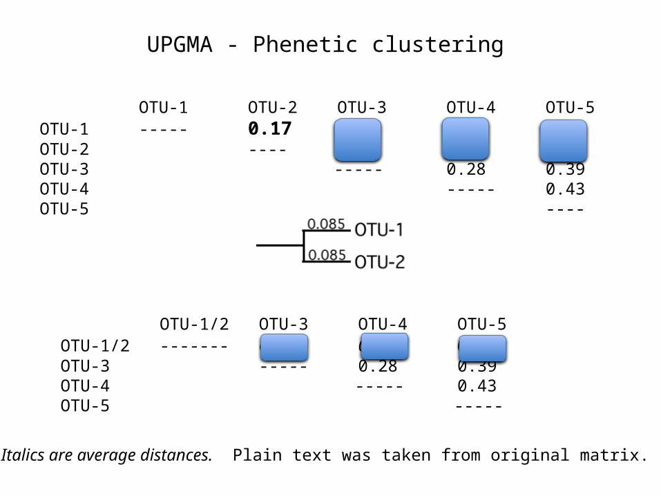
UPGMA - Phenetic clustering
OTU-1 OTU-2 OTU-3 OTU-4 OTU-5
OTU-1 ----- 0.17 0.21 0.31 0.23
OTU-2 ---- 0.30 0.34 0.21
OTU-3 ----- 0.28 0.39
OTU-4 ----- 0.43
OTU-5 ---- OTU-1/2 OTU-3
OTU-4 OTU-5OTU-1/2 ------- 0.255 0.325
0.22OTU-3 -----0.28 0.39OTU-4 ----- 0.43OTU-5
-----
Italics are average distances. Plain text was taken from original matrix.

UPGMA - Phenetic clustering
OTU-1/2 OTU-3OTU-4 OTU-5OTU-1/2 ------- 0.255 0.325
0.22OTU-3 -----0.28 0.39OTU-4 ----- 0.43OTU-5
-----
Again, we erect a new matrix with composite OTU-1/2/5.
The same matrix:

UPGMA - Phenetic clustering
Now in generating the new matrix, we take the unweighted average of the distances (each pairwise distance among members of the composite OTU is weighted equally).
OTU-1/2/5OTU-3 OTU-4OTU-1/2/5 ------------- 0.300
0.360OTU-3 ------- 0.28 OTU-4
-------
D1/2/5,3 = [(0.255 * 2) + 0.39] / 3 = 0.300
D1/2/5,4 = [(0.325 * 2) + 0.43] / 3 = 0.360
UPGMA - Phenetic clustering
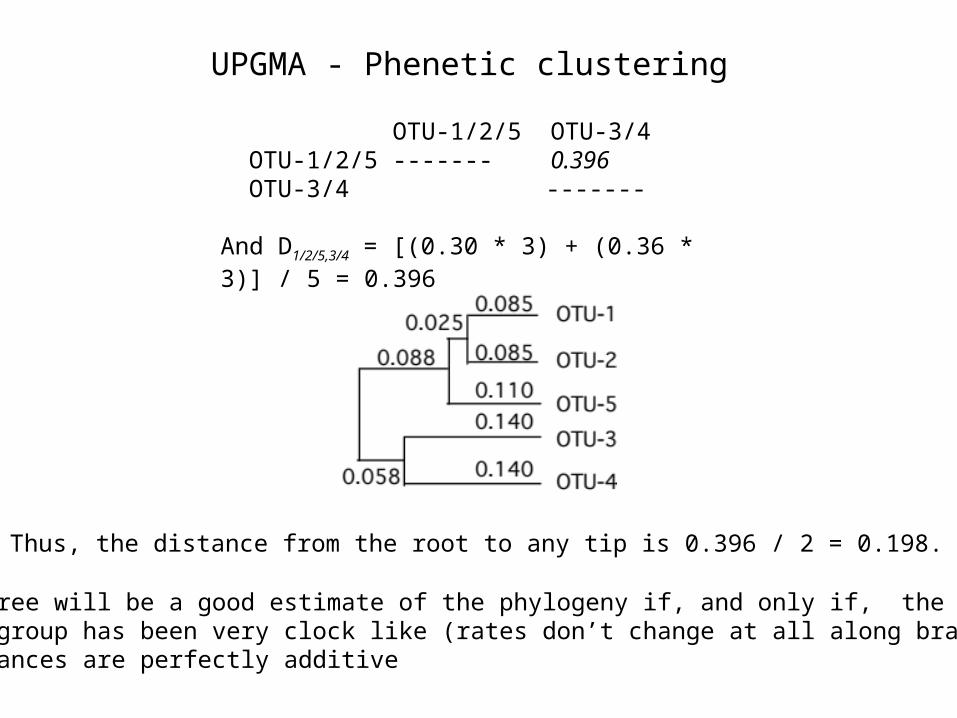
OTU-1/2/5 OTU-3/4
OTU-1/2/5 ------- 0.396OTU-3/4 -------
And D1/2/5,3/4 = [(0.30 * 3) + (0.36 * 3)] / 5 = 0.396
Thus, the distance from the root to any tip is 0.396 / 2 = 0.198.
A UPGMA tree will be a good estimate of the phylogeny if, and only if, the evolution of the group has been very clock like (rates don’t change at all along branches) and if distances are perfectly additive
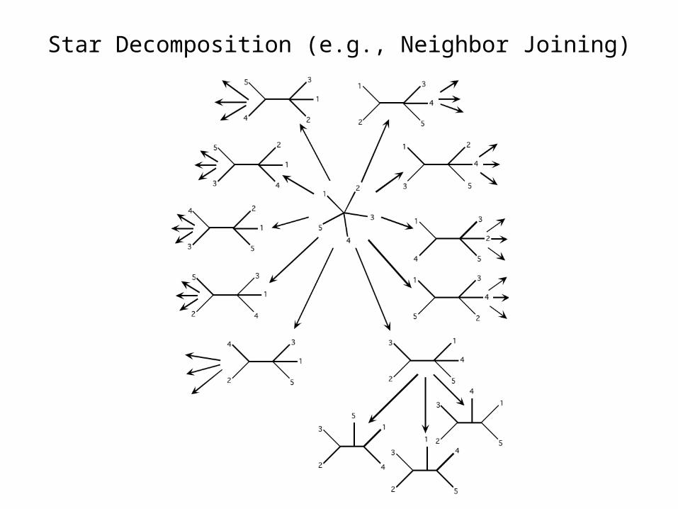
Star Decomposition (e.g., Neighbor Joining)
Star Decomposition – Neighbor Joining
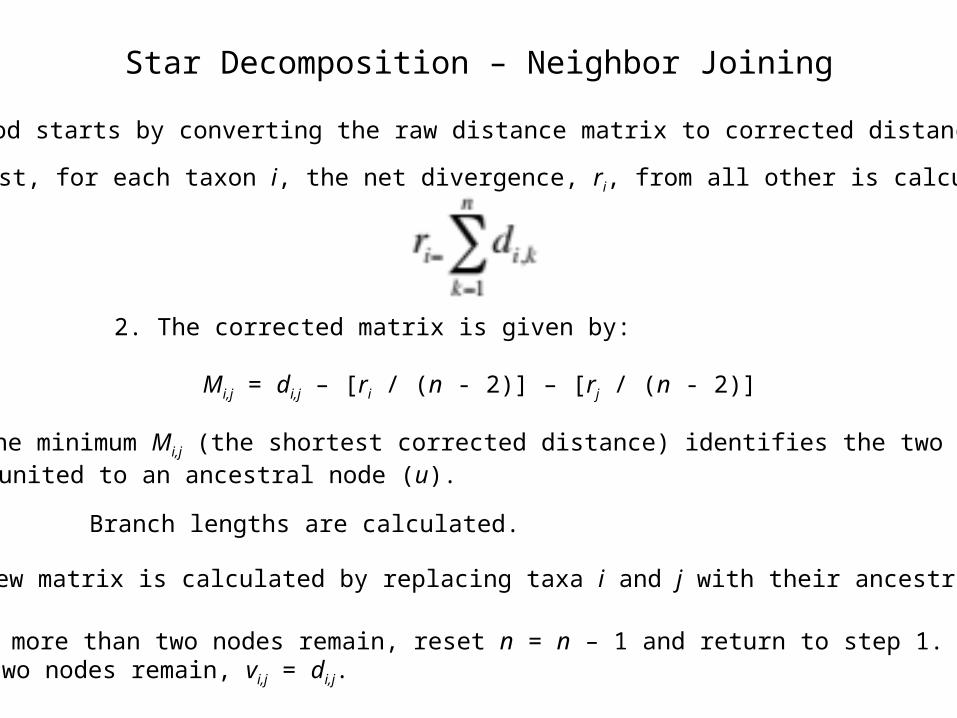
This method starts by converting the raw distance matrix to corrected distance matrix.
1. First, for each taxon i, the net divergence, ri, from all other is calculated.
2. The corrected matrix is given by:
Mi,j = di,j – [ri / (n - 2)] – [rj / (n - 2)]
3. The minimum Mi,j (the shortest corrected distance) identifies the two taxa to be united to an ancestral node (u).
Branch lengths are calculated.
4. A new matrix is calculated by replacing taxa i and j with their ancestral node u.
5. If more than two nodes remain, reset n = n – 1 and return to step 1. If only two nodes remain, vi,j = di,j.

Star Decomposition – Neighbor Joining
A worked example using the same matrix we used for UPGMA
1. First, for each taxon i, the net divergence, ri, from all other is calculated.
2. The corrected matrix is given by:
Mi,j = di,j – [ri / (n - 2)] – [rj / (n - 2)]
OTU-1 OTU-2 OTU-3 OTU-4 OTU-5 ri
ri /(n-2)1 ------- 0.17 0.21
0.31 0.23 0.92 0.3072 -0.477 ------- 0.30 0.34
0.21 1.02 0.3403 -0.490 -0.433 ------- 0.28
0.39 1.18 0.3934 -0.450 -0.453 -0.566 ------- 0.43 1.36 0.4535 -0.497 -0.550 -0.533 -0.443 ------ 1.26 0.420
3. The minimum Mi,j (the shortest corrected distance) identifies the two taxa to be united to an ancestral node (u).
Star Decomposition – Neighbor Joining
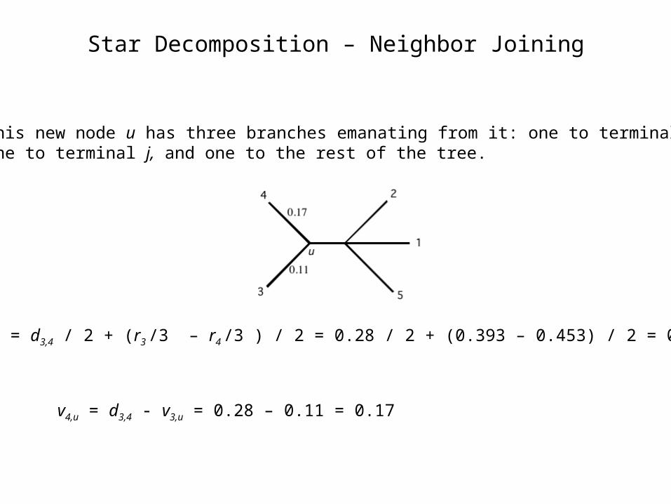
3. This new node u has three branches emanating from it: one to terminal i, one to terminal j, and one to the rest of the tree.
v3,u = d3,4 / 2 + (r3 /3 – r4 /3 ) / 2 = 0.28 / 2 + (0.393 – 0.453) / 2 = 0.11
v4,u = d3,4 - v3,u = 0.28 – 0.11 = 0.17
Star Decomposition – Neighbor Joining
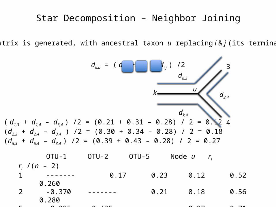
4. A new matrix is generated, with ancestral taxon u replacing i & j (its terminals, 3 & 4).
dk,u = ( di,k + dj,k – di,j ) /2 3
4
uk
dk,3
dk,4
d3,4
d1,u = ( d1,3 + d1,4 – d3,4 ) /2 = (0.21 + 0.31 – 0.28) / 2 = 0.12d2,u = (d2,3 + d2,4 – d3,4 ) /2 = (0.30 + 0.34 – 0.28) / 2 = 0.18d5,u = (d5,3 + d5,4 – d3,4 ) /2 = (0.39 + 0.43 – 0.28) / 2 = 0.27
OTU-1 OTU-2 OTU-5 Node u ri ri /(n – 2)
1 ------- 0.17 0.23 0.12 0.52 0.260
2 -0.370 ------- 0.21 0.18 0.56 0.280
5 -0.385 -0.425 ------- 0.27 0.71 0.355
u -0.425 -0.385 -0.370 ------- 0.57 0.285
Star Decomposition – Neighbor Joining
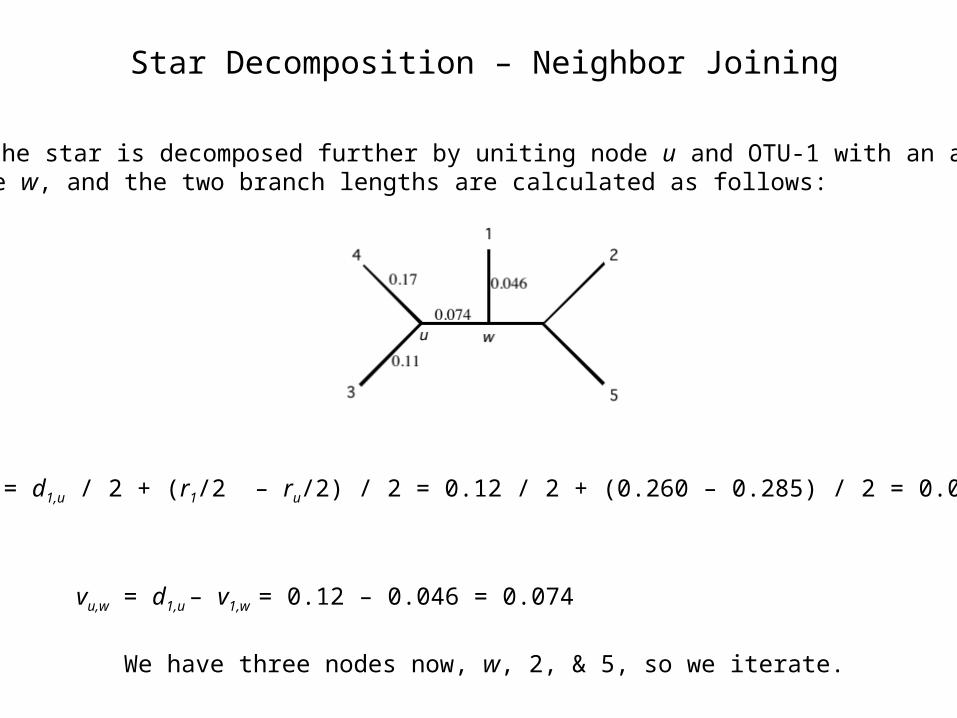
5. So the star is decomposed further by uniting node u and OTU-1 with an ancestral node w, and the two branch lengths are calculated as follows:
v1,w = d1,u / 2 + (r1/2 – ru/2) / 2 = 0.12 / 2 + (0.260 – 0.285) / 2 = 0.046
vu,w = d1,u – v1,w = 0.12 – 0.046 = 0.074
We have three nodes now, w, 2, & 5, so we iterate.
Star Decomposition – Neighbor Joining
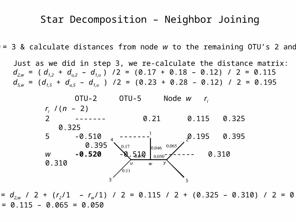
Set n = 3 & calculate distances from node w to the remaining OTU’s 2 and 5.
Just as we did in step 3, we re-calculate the distance matrix:d2,w = ( d1,2 + du,2 – d1,u ) /2 = (0.17 + 0.18 – 0.12) / 2 = 0.115d5,w = (d1,5 + du,5 – d1,u ) /2 = (0.23 + 0.28 – 0.12) / 2 = 0.195
OTU-2 OTU-5 Node w ri ri /(n – 2)2 ------- 0.21 0.1150.325 0.3255 -0.510 ------- 0.1950.395 0.395w -0.520 -0.510 -------0.310 0.310
vy,2 = d2,w / 2 + (r2/1 – rw/1) / 2 = 0.115 / 2 + (0.325 – 0.310) / 2 = 0.065vy,w = 0.115 – 0.065 = 0.050

Star Decomposition – Neighbor Joining
d5,y = ( dw,5 + d2,5 – d2,w ) /2 = (0.195 + 0.21 – 0.115) / 2 = 0.145 = v5,y
Finally, we calculate the distance from node y to OTU –5:
The UPGMA and NJ trees are different for this matrix.
NJ is not phenetic. It is explicitly calculating ancestors and parsing similarity into ancestral vs. derived.
Star Decomposition – Neighbor Joining
An important modification to the neighbor-joining algorithm, BIONJ incorporates variances and covariances of di,j
The number of calculations decreases as we decompose the star tree.
Neighbor joining is often interpreted as an approximation to the ME solution.
Stepwise Addition
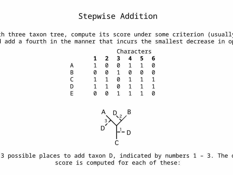
Start with three taxon tree, compute its score under some criterion (usually an ML or MP), and add a fourth in the manner that incurs the smallest decrease in optimality.
Characters1 2
3 4 56
A 1 00 1 10
B 0 01 0 00
C 1 10 1 11
D 1 10 1 11
E 0 01 1 10
There are 3 possible places to add taxon D, indicated by numbers 1 – 3. The optimality score is computed for each of these:
Stepwise Addition
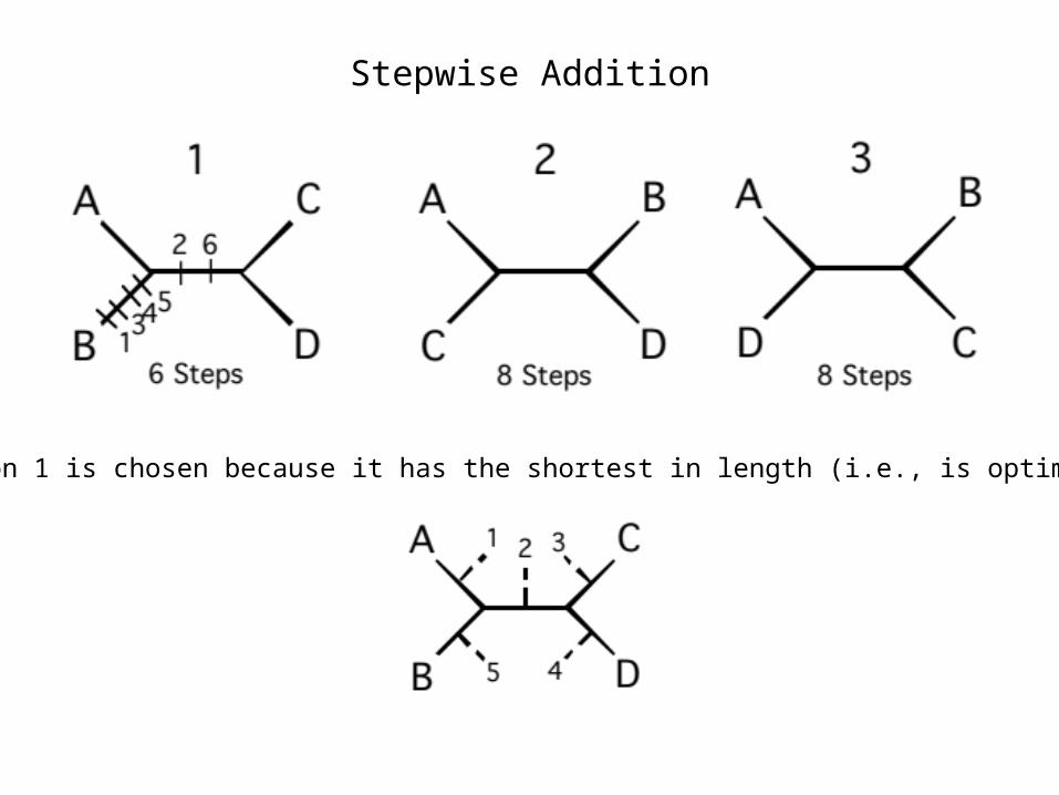
Option 1 is chosen because it has the shortest in length (i.e., is optimal).
Stepwise Addition
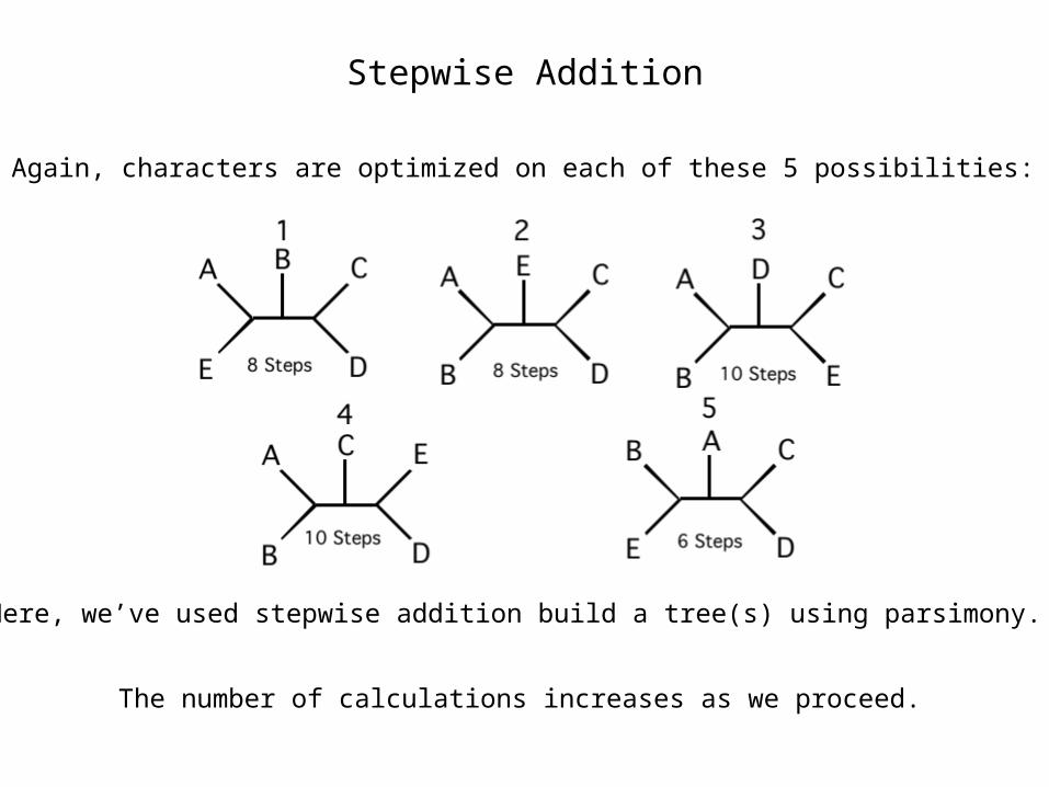
Again, characters are optimized on each of these 5 possibilities:
Here, we’ve used stepwise addition build a tree(s) using parsimony.
The number of calculations increases as we proceed.

Stepwise Addition
Addition sequence is critical. The method is starting-point dependent, so different addition sequences can produce different stepwise addition trees.
Options:
As is – In the order that the taxa appear in the matrix.
Shortest – One may check all triplets, choose that which has the shortest tree and, at each step, assess all candidates, and choose that which adds least length.
Random – One may use random addition sequences and replicate a number of times. For clean data, there should be only small differences in the stepwise addition tree, but for most real data there will be multiple stepwise addition trees. We’ll make use of this in searching tree space.
Quartet Methods
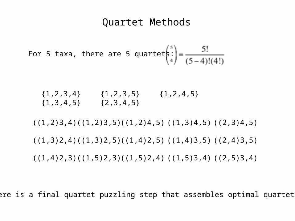
For 5 taxa, there are 5 quartets:
{1,2,3,4} {1,2,3,5} {1,2,4,5} {1,3,4,5}{2,3,4,5}
((1,2)3,4)
((1,3)2,4)
((1,4)2,3)
((1,2)3,5)
((1,3)2,5)
((1,5)2,3)
((1,2)4,5)
((1,4)2,5)
((1,5)2,4)
((1,3)4,5)
((1,4)3,5)
((1,5)3,4)
((2,3)4,5)
((2,4)3,5)
((2,5)3,4)
There is a final quartet puzzling step that assembles optimal quartets.