lecture 6: the casimir operator
TRANSCRIPT
The finite-dimensional case The Kac-Moody inner product The Kac-Moody Casimir operator
Lecture 6: The Casimir operator
Daniel Bump
October 13, 2020
The finite-dimensional case The Kac-Moody inner product The Kac-Moody Casimir operator
The invariant inner product and the Casimir operator
The text for today’s lecture is Kac, Chapter 2. We will constructan invariant bilinear form ( | ) on a Kac-Moody Lie algebra, thenapply it to construct the important Casimir operator onrepresentations of Category O, and prove facts about it thatlead to a proof of the Kac-Weyl character formula for charactersof integrable highest weight representations.
For example, the Casimir operator acts on irreducible highestweight representations as a scalar, which we can compute.This will be of use in locating primitive vectors, among otherthings.
The finite-dimensional case The Kac-Moody inner product The Kac-Moody Casimir operator
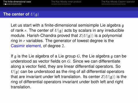
The center of U(g)
Let us start with a finite-dimensional semisimple Lie algebra gof rank r. The center of U(g) acts by scalars in any irreduciblemodule. Harish-Chandra proved that Z(U(g)) is a polynomialring in r variables. The generator of lowest degree is theCasimir element, of degree 2.
If g is the Lie algebra of a Lie group G, the Lie algebra g can beunderstood as vector fields on G. Since we can differentiatealong a vector field, they are linear differential operators. SoU(g) can be understood as the ring of all differential operatorsthat are invariant under left translation. Its center Z(U(g)) is thering of differential operators invariant under both left and righttranslation.

The finite-dimensional case The Kac-Moody inner product The Kac-Moody Casimir operator
The Casimir operator
Let ( | ) be an invariant bilinear form on g, which must be theKilling form up to normalization. Let Xi be a basis of g and let Yi
be the dual basis. Then we may define
Ω =
dim(g)∑i=1
XiYi ∈ U(g).
PropositionThe definition of Ω is independent of the choice of basis Xi, andΩ ∈ Z(U(g)).
The finite-dimensional case The Kac-Moody inner product The Kac-Moody Casimir operator
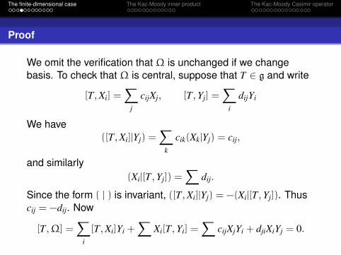
Proof
We omit the verification that Ω is unchanged if we changebasis. To check that Ω is central, suppose that T ∈ g and write
[T,Xi] =∑
j
cijXj, [T,Yj] =∑
i
dijYi
We have([T,Xi]|Yj) =
∑k
cik(Xk|Yj) = cij,
and similarly(Xi|[T,Yj]) =
∑dij.
Since the form ( | ) is invariant, ([T,Xi]|Yj) = −(Xi|[T,Yj]). Thuscij = −dij. Now
[T,Ω] =∑
i
[T,Xi]Yi +∑
Xi[T,Yi] =∑
cijXjYi + djiXiYj = 0.

The finite-dimensional case The Kac-Moody inner product The Kac-Moody Casimir operator
Weight spaces dually paired by ( | )
PropositionLet g be a Lie algebra with a maximal abelian subgroup h.Assume that g has a weight space decomposition
g =⊕α∈h∗
gα.
Assume that ( | ) is an invariant bilinear form. Then if X ∈ gαand Y = gβ we have (X|Y) = 0 unless α = −β.
Indeed, if H ∈ h we have
α(H)(X|Y) = ([H,X]|Y) = −(X|[H,Y]) = −β(H)(X|Y),
so if (X|Y) 6= 0 we must have α(H) = −β(H).

The finite-dimensional case The Kac-Moody inner product The Kac-Moody Casimir operator
The isomorphism ν : h→ h∗
It will be useful to describe Hα (for all positive roots α) anotherway. There is a homomorphism ν : h −→ h∗ associated to theinner pairing ( | ) by
〈H,ν(H ′)〉 = (H|H ′), 〈H, λ〉 = λ(H) = (H|ν−1(λ)).
We may then define an inner product on h∗ by requiring ν to bean isometry. That is,
(ν(H)|ν(H)) = (H|H ′).

The finite-dimensional case The Kac-Moody inner product The Kac-Moody Casimir operator
The scalar value of Ω
Our goal is to prove:
TheoremLet V be an irreducible finite-dimensional module of thefinite-dimensional simple Lie algebra g with highest weightλ ∈ h∗. Then Ω acts on V by the scalar (λ|λ+ 2ρ).
To prove this we will first describe dual bases of g. When α is aroot, Xα (= gα) is one dimensional, and if the basis Xi of g ischosen so that each vector Xi lies in a root space, there will beone vector in each Xα and r vectors in g0 = h. Let us denotethe vectors in Xα by Xα, and the vectors in h by Hi.

The finite-dimensional case The Kac-Moody inner product The Kac-Moody Casimir operator
Normalizations
It will be convenient to adjust the Xα so that (Xα|X−α) = 1.Also, the form ( | ) restricts to a nondegenerate pairing of h, solet Hi be the dual basis of h such that (Hi|Hj) = δij.Now our dual bases Xi and Yi of g may be chosen to beX−α,Hi and Xα,Hi. Thus the Casimir operator is
Ω =∑α∈Φ
X−αXα +
r∑i=1
HiHi.
We will also denote Hα = [Xα,X−α].

The finite-dimensional case The Kac-Moody inner product The Kac-Moody Casimir operator
Computation of Hα
Lemma
We have Hα = ν−1(α).
To check this, we use the fact that the inner product ( | ) isinvariant. We have
(H|[Xα,X−α]) = ([H,Xα]|X−α) = α(H)(Xα|X−a) = α(H).
Now by the definition of ν, this proves thatHα = [Xα,X−α] = ν
−1(α).

The finite-dimensional case The Kac-Moody inner product The Kac-Moody Casimir operator
Another version of Ω
Now we may rewrite
Ω =∑α∈Φ
X−α · Xα +
r∑i=1
HiHi
It is useful to write this in another form using
[Xα,X−α] = Hα = ν−1(α)
by the Lemma, and applying this to those α that are negativeroots:
Ω =∑
α∈Φ+
2X−α · Xα +
r∑i=1
HiHi +∑
α∈Φ+
[Xα,X−α]
or:
Ω =∑
α∈Φ+ 2X−α · Xα +∑r
i=1 HiHi + 2ν−1(ρ).
The finite-dimensional case The Kac-Moody inner product The Kac-Moody Casimir operator
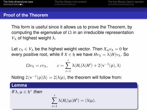
Proof of the Theorem
This form is useful since it allows us to prove the Theorem, bycomputing the eigenvalue of Ω in an irreducible representationVλ of highest weight λ.
Let vλ ∈ Vλ be the highest weight vector. Then Xαvλ = 0 forevery positive root, while if X ∈ h we have Hvλ = λ(H)vλ. So
Ωvλ = cvλ, c =
r∑i=1
λ(Hi)λ(Hi) + 2〈ν−1(ρ), λ〉
Noting 2〈ν−1(ρ)|λ〉 = 2(λ|ρ), the theorem will follow from:
LemmaIf λ,µ ∈ h∗ then
r∑i=1
λ(Hi)µ(Hi) = (λ|µ).
The finite-dimensional case The Kac-Moody inner product The Kac-Moody Casimir operator
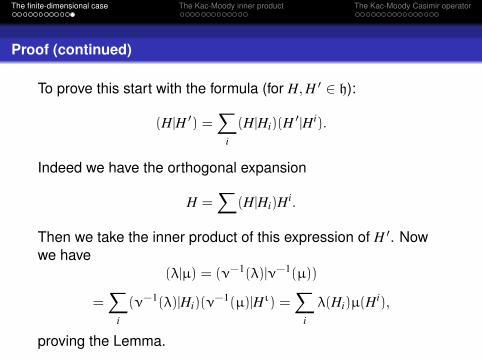
Proof (continued)
To prove this start with the formula (for H,H ′ ∈ h):
(H|H ′) =∑
i
(H|Hi)(H ′|Hi).
Indeed we have the orthogonal expansion
H =∑
(H|Hi)Hi.
Then we take the inner product of this expression of H ′. Nowwe have
(λ|µ) = (ν−1(λ)|ν−1(µ))
=∑
i
(ν−1(λ)|Hi)(ν−1(µ)|Hι) =
∑i
λ(Hi)µ(Hi),
proving the Lemma.
The finite-dimensional case The Kac-Moody inner product The Kac-Moody Casimir operator
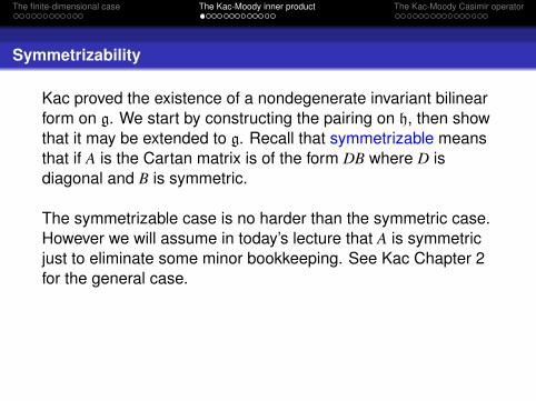
Symmetrizability
Kac proved the existence of a nondegenerate invariant bilinearform on g. We start by constructing the pairing on h, then showthat it may be extended to g. Recall that symmetrizable meansthat if A is the Cartan matrix is of the form DB where D isdiagonal and B is symmetric.
The symmetrizable case is no harder than the symmetric case.However we will assume in today’s lecture that A is symmetricjust to eliminate some minor bookkeeping. See Kac Chapter 2for the general case.
The finite-dimensional case The Kac-Moody inner product The Kac-Moody Casimir operator
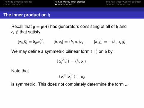
The inner product on h
Recall that g = g(A) has generators consisting of all of h andei, fi that satisfy
[ei, fj] = δijα∨i , [h, ei] = 〈h,αi〉ei, [h, fi] = −〈h,αi〉fi.
We may define a symmetric bilinear form ( | ) on h by
(α∨i |h) = 〈h,αi〉.
Note that(α∨
i |α∨j ) = aji
is symmetric. This does not completely determine the form ...

The finite-dimensional case The Kac-Moody inner product The Kac-Moody Casimir operator
Finishing the inner product on h
Let h ′ =∑
Cα∨i and let h ′′ be a complementary subspace to h ′
in h. Then we may complete the characterization of ( | ) byrequiring that (h ′′|h ′′) = 0.
It is easy to check (since the αi and α∨i are both linearly
independent) that ( | ) is nondegenerate on h.

The finite-dimensional case The Kac-Moody inner product The Kac-Moody Casimir operator
The inner product on g
We have a vector space isomorphism ν : h −→ h ′ determinedby the formula
〈h,ν(h ′)〉 = (h|h ′).
Since (h|α∨i ) = 〈h,αi〉, this implies that
ν(α∨i ) = αi.
Theorem (Theorem 2.2 in Kac)We may extend ( | ) to an invariant bilinear form on g. The formis nondegnerate and satisfies
[x, y] = (x|y)ν−1(α)
if x ∈ Xα, y ∈ X−α.
The finite-dimensional case The Kac-Moody inner product The Kac-Moody Casimir operator
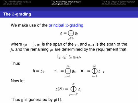
The Z-grading
We make use of the principal Z-grading
g =⊕j∈Z
gj
where g0 = h, g1 is the span of the ei, and g−1 is the span of thefi, and the remaining gk are determined by the requirement that
[gi, gj] ⊆ gi+j.
Thus
h = g0, n+ =
∞⊕i=1
gi, n− =
∞⊕i=1
g−i.
Now let
g(N) =
N⊕j=−N
gj.
Thus g is generated by g(1).
The finite-dimensional case The Kac-Moody inner product The Kac-Moody Casimir operator
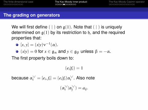
The grading on generators
We will first define ( | ) on g(1). Note that ( | ) is uniquelydetermined on g(1) by its restriction to h, and the requiredproperties that:
[x, y] = (x|y)ν−1(α).(x|y) = 0 for x ∈ gα and y ∈ gβ unless β = −α.
The first property boils down to:
(ei|fi) = 1
because α∨i = [ei, fi] = (ei|fi)α∨
i . Also note
(α∨i |α∨
j ) = aij.
The finite-dimensional case The Kac-Moody inner product The Kac-Moody Casimir operator
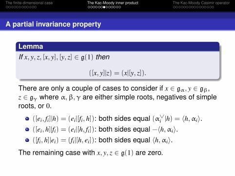
A partial invariance property
LemmaIf x, y, z, [x, y], [y, z] ∈ g(1) then
([x, y]|z) = (x|[y, z]).
There are only a couple of cases to consider if x ∈ gα, y ∈ gβ,z ∈ gγ where α,β,γ are either simple roots, negatives of simpleroots, or 0.
([ei, fi]|h) = (ei|[fi, h]): both sides equal (α∨i |h) = 〈h,αi〉.
([ei, h]|fi) = (ei|[h, fi]): both sides equal −〈h,αi〉.([fi, h]|ei) = (fi|[h, ei]): both sides equal 〈h,αi〉.
The remaining case with x, y, z ∈ g(1) are zero.

The finite-dimensional case The Kac-Moody inner product The Kac-Moody Casimir operator
Expanding the definition
Now we have constructed the invariant inner product ong(1) = h⊕
⊕Cei ⊕
⊕Cfi. This is the base case for an
induction.
LemmaSuppose there exists an inner product ( | ) defined on g(N − 1)subject to the condition that
x, y, z, [x, y], [y, z] ∈ g(N − 1) ⇒ ([x, y]|z) = (x|[y, z]).
Then we may extend it to g(N) with the same property.

The finite-dimensional case The Kac-Moody inner product The Kac-Moody Casimir operator
The recursive definition
It is necessary to define (x|y) when x ∈ g(N) and y ∈ g(−N). Weassume that x, y are homogenous, that is, lie in weight spaces.We may write y =
∑i[ui, vi] where ui and vi are in g(N−1) and
are homogeneous. Then we define
(x|y) =∑
i
([x, ui]|vi).
Note that [x, ui] is homogeneous since x, ui are. It is understoodthat since vi ∈ g(N − 1), the term ([x, ui]|vi) is interpreted as zeroif [x, ui] is not in g(N − 1).
It must be checked that this expression is well-defined,independent of the decomposition y =
∑[ui, vi].
The finite-dimensional case The Kac-Moody inner product The Kac-Moody Casimir operator
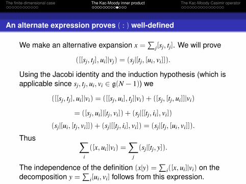
An alternate expression proves ( : ) well-defined
We make an alternative expansion x =∑
j[sj, tj]. We will prove
([[sj, tj], ui]|vj) = (sj|[tj, [ui, vi]]).
Using the Jacobi identity and the induction hypothesis (which isapplicable since sj, tj, ui, vi ∈ g(N − 1)) we
([[sj, tj], ui]|vi) = ([[sj, ui], tj]|vi) + ([sj, [tj, ui]]|vi)
= ([sj, ui]|[tj, vi]) + (sj|[[tj, ii], vi])
(sj|[ui, [tj, vi]]) + (sj|[[tj, ii], vi]) = (sj|[tj, [ui, vi]]).
Thus ∑i
([x, ui]|vi) =∑
j
(sj|[tj, y]).
The independence of the definition (x|y) =∑
i([x, ui]|vi) on thedecomposition y =
∑i[ui, vi] follows from this expression.
The finite-dimensional case The Kac-Moody inner product The Kac-Moody Casimir operator
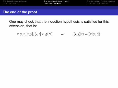
The end of the proof
One may check that the induction hypothesis is satisfied for thisextension, that is:
x, y, z, [x, y], [y, z] ∈ g(N) ⇒ ([x, y]|z) = (x|[y, z]).
The finite-dimensional case The Kac-Moody inner product The Kac-Moody Casimir operator
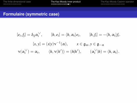
Formulaire (symmetric case)
[ei, fj] = δijα∨i , [h, ei] = 〈h,αi〉ei, [h, fi] = −〈h,αi〉fi.
[x, y] = (x|y)ν−1(α), x ∈ gα, y ∈ g−α
ν(α∨i ) = αi, 〈h,ν(h ′)〉 = (h|h ′), (α∨
i |h) = 〈h,αi〉.
The finite-dimensional case The Kac-Moody inner product The Kac-Moody Casimir operator
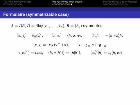
Formulaire (symmetrizable case)
A = DB, D = diag(ε1, · · · , εn), B = (bij) symmetric
[ei, fj] = δijα∨i , [h, ei] = 〈h,αi〉ei, [h, fi] = −〈h,αi〉fi.
[x, y] = (x|y)ν−1(α), x ∈ gα, y ∈ g−α
ν(α∨i ) = εiαi, 〈h,ν(h ′)〉 = (h|h ′), (α∨
i |h) = εi〈h,αi〉

The finite-dimensional case The Kac-Moody inner product The Kac-Moody Casimir operator
First definition
Now let us develop the Casimir element in the Kac-Moodycase. It is not to be an element of U(g), though it can bedefined for a completion of U(g). Instead, as in Chapter 2 ofKac’ book, the Casimir element will be an operator that can bedefined for representations of Category O.
In the Kac-Moody case some spaces gα = Xα may havedimension > 1 so we should choose a basis X(t)
α such that thatX(t)−α is to be the dual basis and formally write:
Ω =∑α∈Φ
dim(Xα)∑t=1
X(t)α · X(t)
−α +
r∑i=1
HiHi.
(For real roots Xα will be one-dimensional, but for imaginaryroots the dimension may be > 1 as in the affine case.)
The finite-dimensional case The Kac-Moody inner product The Kac-Moody Casimir operator
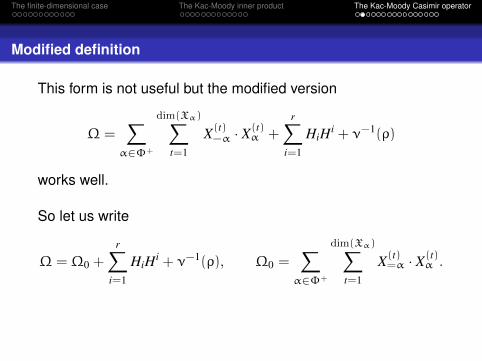
Modified definition
This form is not useful but the modified version
Ω =∑
α∈Φ+
dim(Xα)∑t=1
X(t)−α · X
(t)α +
r∑i=1
HiHi + ν−1(ρ)
works well.
So let us write
Ω = Ω0 +
r∑i=1
HiHi + ν−1(ρ), Ω0 =∑
α∈Φ+
dim(Xα)∑t=1
X(t)=α · X(t)
α .

The finite-dimensional case The Kac-Moody inner product The Kac-Moody Casimir operator
Why it works
LemmaLet V be a representation in Category O and let v ∈ V. ThenX(t)α v = 0 for all but finitely many α.
By definition of Category O there are a finite number ofλ1, · · · , λN ∈ h∗ such that if Vµ 6= 0 then µ 4 λi for some i. Forexample if V is a highest weight representation with highestweight λ we may take N = 1 and λ1 = λ.
Now let v ∈ V have weight µ. Then Xαv has weight µ+ α.There are only a finite number of positive roots α such thatµ+ α 4 λi, so Xαv = 0 for all but finitely many α. Thus the sum∑
X−αXαv is actually finite.
The finite-dimensional case The Kac-Moody inner product The Kac-Moody Casimir operator
Normal ordering
In physics one encounters the notion of “normal ordering”which may be summed up with the admonish to performannihilation operators before creation operators. In physics theoperators are applied to a Hilbert space representing the stateof a physical system and there are operators that create orannihilate particles. Normal ordering is the procedure of alwaysapplying annihilation operators before creation operators. Thisallows one to work with series that would otherwise bedivergent. Normal ordering is also a source of the centralextensions of infinite-dimensional Lie algebras that often popup. In the context of representations in Category O, theoperators Xα with α ∈ Φ+ are annihilation operators, and theoperators X−α are creation operators, writing Ω this way is aperfect example of normal ordering.
The finite-dimensional case The Kac-Moody inner product The Kac-Moody Casimir operator
Normal ordering (continued)
The operator Ω0 makes sense applied to any vector in arepresentation V in Category O, since the sum
∑X(t)−αX(t)
α v hasonly finitely many nonzero terms. Hence the Casimir operator isdefined.
In Category O we may think of Xα as an annihilation operator ifα is a positive root, and as a creation operator when α is anegative root. So when we write
Ω0 =∑
α∈Φ+
dim(Xα)∑i=1
2X(i)−α · X
(i)α ,
this is an example of normal ordering.
The finite-dimensional case The Kac-Moody inner product The Kac-Moody Casimir operator
si permutes Φ+ − αi
LemmaLet si be a simple reflection. If α is a positive root, thensi(α) = −α if α = αi; otherwise si(α) is positive.
To prove this we note that the positive roots are the weightspaces in n+. It is spanned by elements of the form
[ei1 [ei2,[ei3 , · · · , [eik−1 , eik ]]]].
From this description, the positive roots have the form
α =
r∑j=1
kjαj
where (k1, · · · , kr) is a tuple of nonnegative integers.
The finite-dimensional case The Kac-Moody inner product The Kac-Moody Casimir operator
Proof (continued)
The weight kαi is only a root if k = 1, because [αi,αi] = 0, so ifthe above expression has all i1, i2, · · · = i we must have k = 1.Now apply si to
∑kiαi to obtain
si(α) =∑
kjαj − 〈α∨i ,α〉αi =
r∑j=1
k ′jαj
where k ′j = kj if j 6= i. If α 6= αi at least one kj = k ′j is positive, sosi(α) cannot be a negative root.

The finite-dimensional case The Kac-Moody inner product The Kac-Moody Casimir operator
The Weyl vector
Now let us consider the Weyl vector ρ = 12
∑α∈Φ+ α, which we
treat as a divergent sum to be renormalized. Since si sends αi
to −αi and permutes the remaining positive roots, we have(formally) si(ρ) = ρ− αi. Remembering that
sα(x) = x − 〈α∨, x〉α
we need ρ to be an element of the weight lattice P such that
〈α∨i , ρ〉 = 1 for simple roots αi.
This does not quite fully characterize ρ since the α∨ do notspan h in the Kac-Moody case. However this is the onlyproperty that we need ρ to have. We choose ρ ∈ h∗ to be afixed element with this property.

The finite-dimensional case The Kac-Moody inner product The Kac-Moody Casimir operator
What we will prove
We may now state our goals. For representations of CategoryO :
We will prove that Ω commutes with the action of the ei
and fi.Therefore it acts as a scalar on irreducible representations.For highest weight representations we may compute thisscalar.This will contain enough information to help prove theKac-Weyl character formula.
The finite-dimensional case The Kac-Moody inner product The Kac-Moody Casimir operator
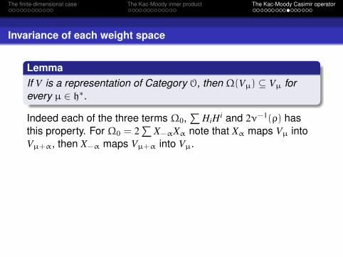
Invariance of each weight space
LemmaIf V is a representation of Category O, then Ω(Vµ) ⊆ Vµ forevery µ ∈ h∗.
Indeed each of the three terms Ω0,∑
HiHi and 2ν−1(ρ) hasthis property. For Ω0 = 2
∑X−αXα note that Xα maps Vµ into
Vµ+α, then X−α maps Vµ+α into Vµ.
The finite-dimensional case The Kac-Moody inner product The Kac-Moody Casimir operator
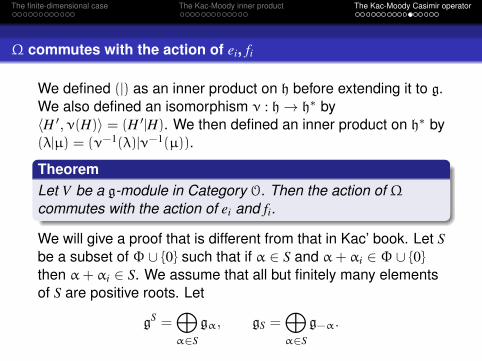
Ω commutes with the action of ei, fi
We defined (|) as an inner product on h before extending it to g.We also defined an isomorphism ν : h→ h∗ by〈H ′,ν(H)〉 = (H ′|H). We then defined an inner product on h∗ by(λ|µ) = (ν−1(λ)|ν−1(µ)).
TheoremLet V be a g-module in Category O. Then the action of Ωcommutes with the action of ei and fi.
We will give a proof that is different from that in Kac’ book. Let Sbe a subset of Φ ∪ 0 such that if α ∈ S and α+ αi ∈ Φ ∪ 0then α+ αi ∈ S. We assume that all but finitely many elementsof S are positive roots. Let
gS =⊕α∈S
gα, gS =⊕α∈S
g−α.

The finite-dimensional case The Kac-Moody inner product The Kac-Moody Casimir operator
Proof
The spacesgS =
⊕α∈S
gα, gS =⊕α∈S
g−α.
are dually paired under ( | ) so let Xt be a basis of gS and Xt bethe dual basis of gS. Define
ΩS =∑
t
XtXt.
We will prove that ei commutes with ΩS. Since all but finitelymany of the Xt are in n+, this makes sense as an operator on V.
Note that [ei, gS] ⊆ gS and [ei, gS] ⊆ gS. We write
[ei,Xt] =∑
u
ctuXu, [ei,Xt] =∑
u
dtuXu.

The finite-dimensional case The Kac-Moody inner product The Kac-Moody Casimir operator
Proof (continued)
Using the fact that Xu is the dual basis of Xt
ctu = ([ei,Xt]|Xu), dtu = (Xu|[ei,Xt]).
Since ( | ) is invariant, we have ctu = −dut. Now[ei,
∑t
XtXt
]=
∑t
[ei,Xt]Xt +∑
t
Xt[ei,Xt].
This equals ∑t,u
ctuXuXt +∑t,u
dtuXtXu = 0.
We have proved that [ei,ΩS] = 0.
We will apply this twice.
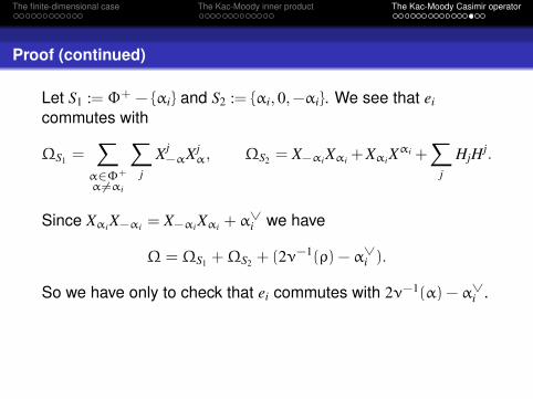
The finite-dimensional case The Kac-Moody inner product The Kac-Moody Casimir operator
Proof (continued)
Let S1 := Φ+ − αi and S2 := αi, 0,−αi. We see that ei
commutes with
ΩS1 =∑
α∈Φ+
α6=αi
∑j
Xj−αXj
α, ΩS2 = X−αiXαi +XαiXαi +
∑j
HjHj.
Since XαiX−αi = X−αiXαi + α∨i we have
Ω = ΩS1 +ΩS2 + (2ν−1(ρ) − α∨i ).
So we have only to check that ei commutes with 2ν−1(α) − α∨i .
The finite-dimensional case The Kac-Moody inner product The Kac-Moody Casimir operator
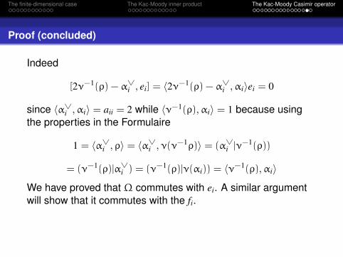
Proof (concluded)
Indeed
[2ν−1(ρ) − α∨i , ei] = 〈2ν−1(ρ) − α∨
i ,αi〉ei = 0
since 〈α∨i ,αi〉 = aii = 2 while 〈ν−1(ρ),αi〉 = 1 because using
the properties in the Formulaire
1 = 〈α∨i , ρ〉 = 〈α∨
i ,ν(ν−1ρ)〉 = (α∨i |ν−1(ρ))
= (ν−1(ρ)|α∨i ) = (ν−1(ρ)|ν(αi)) = 〈ν−1(ρ),αi〉
We have proved that Ω commutes with ei. A similar argumentwill show that it commutes with the fi.

The finite-dimensional case The Kac-Moody inner product The Kac-Moody Casimir operator
The main theorem
TheoremSuppose V is a highest weight representation with highestweight λ. Then Ω acts as a scalar on V, with value (λ|λ+ 2ρ).
Let vλ be the highest weight vector. Since X(t)α annihilates vλ we
have to compute the eigenvalue of∑i
(HiHi) + 2ν−1(ρ)
on vλ. The calculations that show this is (λ|λ) + 2(λ|ρ) areidentical to the finite-dimensional simple case.