lecture 6: interpolation - fatih guvenen guvenen ( ) lecture 6: interpolation january 10, 2016 2 /...
TRANSCRIPT

Lecture 6: Interpolation
Fatih Guvenen
January 10, 2016
Fatih Guvenen ( ) Lecture 6: Interpolation January 10, 2016 1 / 25

General Idea
Suppose you are given a grid (x1, x2,..., xn) and the function values(y1, y2, ..., yn) at corresponding points generated by function f (x)
Q: How to find values off the grid points that provides a “goodapproximation” to f (x)?
A good approximation is often taken to mean to minimize���f (x)�bf (x)��� according to some norm (Lp, sup-, etc).
In economics another very important concern is to preserve theshape—ie, concavity or convexity—of the interpolated (e.g, utilityor value) function
Popular methods are linear-, Chebyshev-, and Spline-interpolations. I will spend most of my time on Splines.
Fatih Guvenen ( ) Lecture 6: Interpolation January 10, 2016 2 / 25

Polynomial Approximation
Weierstrass Approximation Theorem. Suppose f is acontinuous real-valued function defined on the real interval [a, b].For a given " > 0, there exists a polynomial of order n, Pn(x), suchthat for all x in [a, b], we have kf (x)� Pn(x)k1 < ". In the limit,
limn!1
kf (x)� Pn(x)k1 = 0.
Runge. Let f (x) = 1/(1 + x2) on [-5,5], and let Lmf be the uniquepolynomial of order m that interpolates f at m equally-spacedpoints. Then:
lim supm!1
|f (x)� Lmf | =(
0 if |x | < 3.633...,1 if |x | > 3.633...
The two theorems are not contradictory. The first theorem doesnot provide a way of finding the right Pn(x) and the second oneshows a naive approach can fail spectacularly.
Fatih Guvenen ( ) Lecture 6: Interpolation January 10, 2016 3 / 25

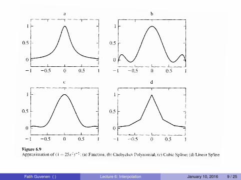
Runge Example
Splines: Three Objectives
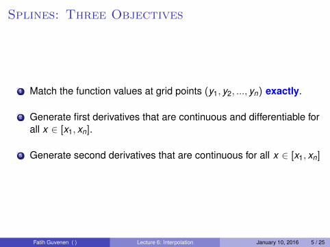
1 Match the function values at grid points (y1, y2, ..., yn) exactly.
2 Generate first derivatives that are continuous and differentiable forall x 2 [x1, xn].
3 Generate second derivatives that are continuous for all x 2 [x1, xn]
Fatih Guvenen ( ) Lecture 6: Interpolation January 10, 2016 5 / 25

Splines: Building from Ground Up
Begin with the interval between two generic knots, xi and xi+1. Ifwe were to construct a linear interpolant:
y = Ayj + Byj+1
A(x) ⌘xj+1 � xxj+1 � xj
B(x) ⌘ 1 � A =x � xj
xj+1 � xj(1)
Although linear interpolation is sometimes useful, a shortcomingis that
I First derivative changes abruptly at the knot points, i.e., theinterpolants have as many kinks as the knot points.
I Second derivative does not exist at knot points.
This can create many problems, such as difficulties with derivativebased minimization algorithms.Question: How can we modify (1) to allow differentiable firstderivatives and continuous second derivatives at all points?
Fatih Guvenen ( ) Lecture 6: Interpolation January 10, 2016 6 / 25
Splines: Building from Ground Up
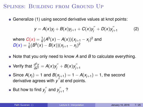
Generalize (1) using second derivative values at knot points:
y = A(x)yj + B(x)yj+1 + C(x)y00j + D(x)y
00j+1 (2)
where C(x) = 16(A
3(x)� A(x))(xj+1 � xj)2 and
D(x) = 16(B
3(x)� B(x))(xj+1 � xj)2
Note that you only need to know A and B to calculate everything.
Verify that d2ydx2 = A(x)y
00j + B(x)y
00j+1
Since A(xj) = 1 and B(xj+1) = 1 � A(xj+1) = 1, the secondderivative agrees with y
00at end points.
But how to find y00j and y
00j+1 ?
Fatih Guvenen ( ) Lecture 6: Interpolation January 10, 2016 7 / 25
Splines: Building from Ground Up
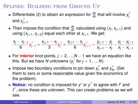
Differentiate (2) to obtain an expression for dydx that will involve y
00j
and y00j+1.
Then impose the condition that dydx calculated using (xj , xj+1) and
using (xj+1, xj+2) equal each other at xj+1. We get:
xj � xj�1
6y
00j�1 +
xj+1 � xj
3y
00j +
xj+1 � xj
6y
00j+1 =
yj+1 � yj
xj+1 � xj�
yj � yj�1
xj � xj�1
For interior knot points, j = 2, ...,N � 1 we have an equation likethis. But we have N unknowns (y”
j for j = 1, ...,N).
Impose two boundary conditions to pin down y001 and y
00N . (Set
them to zero or some reasonable value given the economics ofthe problem).Notice: no condition is imposed for y 0 or y
00 to agree with f 0 andf00 , since these are unknown. This can create problems as we will
see.Fatih Guvenen ( ) Lecture 6: Interpolation January 10, 2016 8 / 25
Fatih Guvenen ( ) Lecture 6: Interpolation January 10, 2016 9 / 25
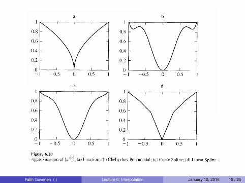
Fatih Guvenen ( ) Lecture 6: Interpolation January 10, 2016 10 / 25

Comparing InterpolationMethods for U(C)

Comparing Boundary Conditions
Figure: N = 500 pts
0.04 0.06 0.08 0.1 0.12 0.14 0.16
Log
Axis
-1011
-1010
-109
-108
-107
-106
y′
1 = U′
(0.05)y
′
1 = 0Natural SplineTrue Function
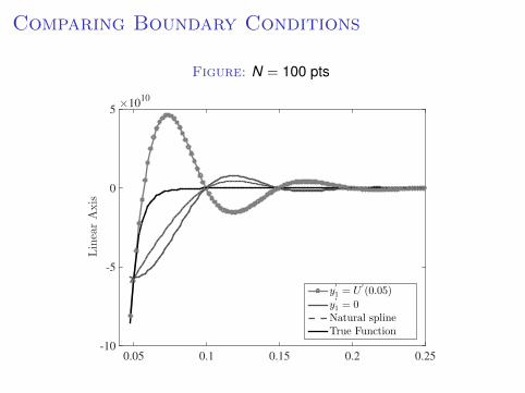
Comparing Boundary Conditions
Figure: N = 100 pts
0.05 0.1 0.15 0.2 0.25
LinearAxis
×1010
-10
-5
0
5
y′
1 = U′
(0.05)y
′
1 = 0Natural splineTrue Function

Interpolation: What Can Go Wrong
0 0.5 1 1.5 2−1
−0.5
0
0.5
1
1.5
2x 10
8
CRRA function with γ = 10
8th-order polynomial
Cubic spline
Shumaker quadratic spline
Fatih Guvenen ( ) Lecture 6: Interpolation January 10, 2016 14 / 25
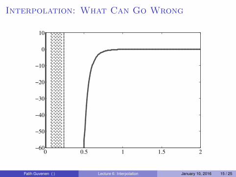
Interpolation: What Can Go Wrong
0 0.5 1 1.5 2−60
−50
−40
−30
−20
−10
0
10
Fatih Guvenen ( ) Lecture 6: Interpolation January 10, 2016 15 / 25
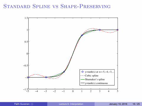
Standard Spline vs Shape-Preserving
−5 −4 −3 −2 −1 0 1 2 3 4 5−1.5
−1
−0.5
0
0.5
1
1.5
y=tanh(x) at x=−5,−4,−3,...
Cubic spline
Shumaker’s spline
y=tanh(x) continuous
Fatih Guvenen ( ) Lecture 6: Interpolation January 10, 2016 16 / 25
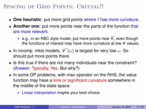
Spacing of Grid Points: Crucial!!
One heuristic: put more grid points where f has more curvature.Another one: put more points near the parts of the function thatare more relevant.
I e.g., in an RBC style model, put more points near K , even thoughthe functions of interest may have more curvature at low K values.
In incomp. mkts models, V00(!) is largest for very low !. So
should put more points there.Is this true if there are not many individuals near the constraint?(Answer: Typically, Yes. But why?)In some DP problems, with max operator on the RHS, the valuefunction may have a kink or significant curvature somewhere inthe middle of the state space.
I Linear interpolation maybe your best choice.
Fatih Guvenen ( ) Lecture 6: Interpolation January 10, 2016 17 / 25
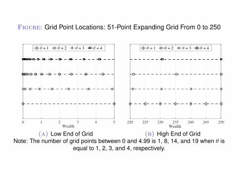
Figure: Grid Point Locations: 51-Point Expanding Grid From 0 to 250
Wealth
0 1 2 3 4 5
θ = 1 θ = 2 θ = 3 θ = 4
(a) Low End of GridWealth
220 225 230 235 240 245 250
θ = 1 θ = 2 θ = 3 θ = 4
(b) High End of GridNote: The number of grid points between 0 and 4.99 is 1, 8, 14, and 19 when ✓ is
equal to 1, 2, 3, and 4, respectively.
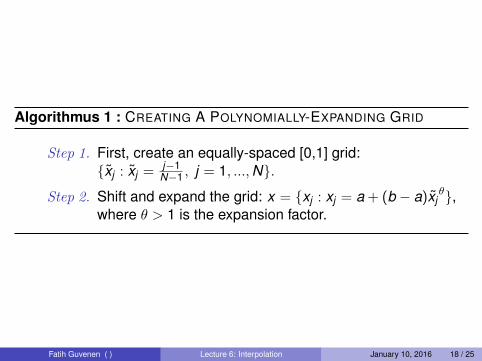
Algorithmus 1 : CREATING A POLYNOMIALLY-EXPANDING GRID
Step 1. First, create an equally-spaced [0,1] grid:{x̃j : x̃j =
j�1N�1 , j = 1, ...,N}.
Step 2. Shift and expand the grid: x = {xj : xj = a + (b � a)x̃j✓},
where ✓ > 1 is the expansion factor.
Fatih Guvenen ( ) Lecture 6: Interpolation January 10, 2016 18 / 25

Spline w/ Expanding Grid(1000 pts)
Figure: N = 1000 pts
0 0.2 0.4 0.6 0.8 1-100
-50
0
50
100
Equally-spaced, θ =1.0
θ = 1.05
θ = 1.10
Fatih Guvenen ( ) Lecture 6: Interpolation January 10, 2016 19 / 25

Spline w/ Expanding Grid (100 pts)
Figure: N = 100 pts
0 1 2 3 4 5-10
-5
0
5
10
U(C)
θ = 1.0
θ = 2.0
θ = 3.0
Fatih Guvenen ( ) Lecture 6: Interpolation January 10, 2016 20 / 25
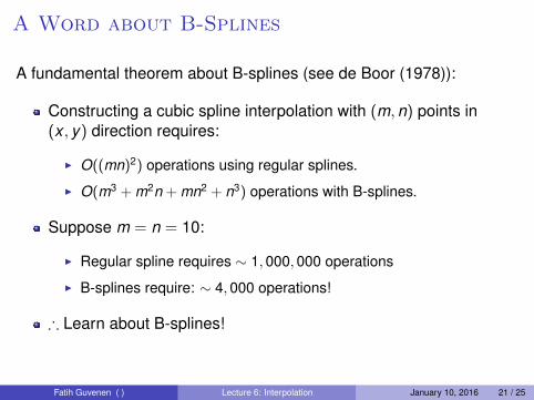
A Word about B-Splines
A fundamental theorem about B-splines (see de Boor (1978)):
Constructing a cubic spline interpolation with (m, n) points in(x , y) direction requires:
I O((mn)2) operations using regular splines.
I O(m3 + m2n + mn2 + n3) operations with B-splines.
Suppose m = n = 10:
I Regular spline requires ⇠ 1, 000, 000 operations
I B-splines require: ⇠ 4, 000 operations!
) Learn about B-splines!
Fatih Guvenen ( ) Lecture 6: Interpolation January 10, 2016 21 / 25
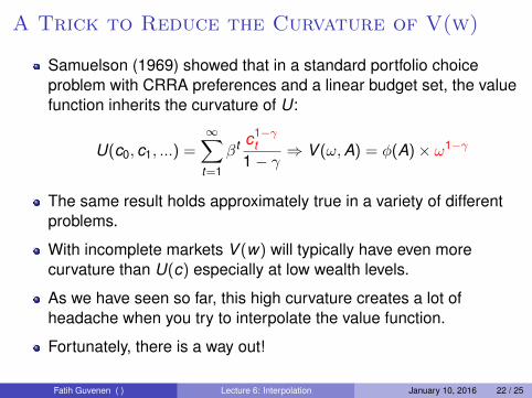
A Trick to Reduce the Curvature of V(w)
Samuelson (1969) showed that in a standard portfolio choiceproblem with CRRA preferences and a linear budget set, the valuefunction inherits the curvature of U:
U(c0, c1, ...) =1X
t=1
�t c1��t
1 � �) V (!,A) = �(A)⇥ !1��
The same result holds approximately true in a variety of differentproblems.
With incomplete markets V (w) will typically have even morecurvature than U(c) especially at low wealth levels.
As we have seen so far, this high curvature creates a lot ofheadache when you try to interpolate the value function.
Fortunately, there is a way out!
Fatih Guvenen ( ) Lecture 6: Interpolation January 10, 2016 22 / 25

A Trick to Reduce the Curvature of V(w)
There is an alternative formulation of CRRA preferences:
U(c0, c1, ...) =
1X
t=1
�t c(1��)t
!1/(1��)
This is a special case of Epstein-Zin (1989, E’trica) utility andrepresents the same preferences as CRRA utility with RRA = ⇢.
Now the value function is linear: V (!,A) = �(A)⇥ !
Although incomplete markets introduces some curvature, thisvalue function is much easier to interpolate than the one above.
In fact, I once solved a GE model with asset pricing and a riskaversion of 4 using only 30 points in the wealth grid and linearinterpolation!
Fatih Guvenen ( ) Lecture 6: Interpolation January 10, 2016 23 / 25

0 1 2 3 4 5-10
15
-1010
-105
-100
-10-5
-10-10
0 1 2 3 4 5
0.19
0.20
0.21
Epstein-Zin Value Func.(right axis)
Standard CRRA Utility(left axis)
Figure: Which Function Would You Rather Interpolate?
Fatih Guvenen ( ) Lecture 6: Interpolation January 10, 2016 24 / 25
Final Thoughts
For any model that you solve, you MUST eventually re-solve it ona much finer grid and confirm that your main results are notchanging (much).
This is the only realistic way to check if approximation errorscoming from interpolations are important.
You will be surprised to find that some bad-looking interpolationsactually yield the same results as much more accurate (and morecostly to compute) interpolations.
And vice versa..Some problems are especially sensitive to any kind ofapproximation errors. We will see examples.
Fatih Guvenen ( ) Lecture 6: Interpolation January 10, 2016 25 / 25