lecture 6: income and wealth distributionmoll/eco521web/lecture6_eco521_web.pdflecture 6: income and...
TRANSCRIPT

Lecture 6: Income and Wealth Distribution
ECO 521: Advanced Macroeconomics I
Benjamin Moll
Princeton University
Fall 2012

Outline
(1) Some empirical evidence
(2) Benhabib, Bisin and Zhu (2012)
(3) Benhabib, Bisin and Zhu (2011)
(4) Other related literature

Empirical Evidence
• Will focus on inequality at top of income and wealth
distribution
• Nice summary of facts: Atkinson, Piketty, and Saez (2011),
”Top Incomes in the Long Run of History,” Journal of
Economic Literature
• Coined the term “the 1 percent”
• Good example of Keynes’ quote: “The ideas of economists and
political philosophers, both when they are right and when they are wrong,
are more powerful than is commonly understood. Indeed the world is
ruled by little else. Practical men, who believe themselves to be quite
exempt from any intellectual influence, are usually the slaves of some
defunct economist”

Evolution of Top Incomes
Figure 1. The Top Decile Income Share in the United States, 1917–2007.
Notes: Income is de!ned as market income including realized capital gains (excludes government transfers). In 2007, top decile includes all families with annual income above $109,600.
Source: Piketty and Saez (2003), series updated to 2007.
25%
30%
35%
40%
45%
50%
1917
1922
1927
1932
1937
1942
1947
1952
1957
1962
1967
1972
1977
1982
1987
1992
1997
2002
2007
Sh
are
of t
otal
inco
me
goin
g to
Top
10%

Evolution of Top Incomes
0%
5%
10%
15%
20%
25%
1913
1918
1923
1928
1933
1938
1943
1948
1953
1958
1963
1968
1973
1978
1983
1988
1993
1998
2003
Sh
are
of t
otal
inco
me
accr
uin
g to
eac
h g
rou
p
Top 1% (incomes above $398,900 in 2007)
Top 5–1% (incomes between $155,400 and $398,900)
Top 10–5% (incomes between $109,600 and $155,400)
Figure 2. Decomposing the Top Decile US Income Share into three Groups, 1913–2007
Notes: Income is de!ned as market income including capital gains (excludes all government transfers). Top 1 percent denotes the top percentile (families with annual income above $398,900 in 2007).Top 5–1 percent denotes the next 4 percent (families with annual income between $155,400 and $398,900 in 2007).Top 10–5 percent denotes the next 5 percent (bottom half of the top decile, families with annual income between $109,600 and $155,400 in 2007).

Evolution of Top Incomes
0%
2%
4%
6%
8%
10%
12%
1916
1921
1926
1931
1936
1941
1946
1951
1956
1961
1966
1971
1976
1981
1986
1991
1996
2001
2006
Capital Gains
Capital Income
Business Income
Salaries
Figure 3. The Top 0.1 Percent Income Share and Composition, 1916–2007
Notes: The �gure displays the top 0.1 percent income share and its composition. Income is de�ned as market income including capital gains (excludes all government transfers). Salaries include wages and salaries, bonus, exercised stock-options, and pensions. Business income includes pro�ts from sole proprietorships, partnerships, and S-corporations. Capital income includes interest income, dividends, rents, royalties, and �duciary income. Capital gains includes realized capital gains net of losses.

Cross-Country Evidence
• In practice, quite often don’t have data on share of top 1%
• Use Pareto interpolation. Assume income has CDF
F (y) = 1−(y
k
)
−α
• Useful property of Pareto distribution: average above
threshold proportional to threshold
E[y |y ≥ y ] =
∫
∞
yzf (z)dz
1− F (y)=
α
α− 1y
• Estimate and report β ≡ α/(α − 1).
• Example: β = 2 means average income of individuals with
income above $100,000 is $200,000 and average income of
individuals with income above $1 million is $2 million.
• Obviously imperfect, but useful because α or β is exactly
what our theories generate.

Cross-Country Evidence
TABLE 6Comparative Top Income Shares
Around 1949 Around 2005
Share of top 1%
Share of top 0.1%
β coef!cient
Share of top 1%
Share of top 0.1%
β coef!cient
Indonesia 19.87 7.03 2.22
Argentina 19.34 7.87 2.56 16.75 7.02 2.65
Ireland 12.92 4.00 1.96 10.30 2.00
Netherlands 12.05 3.80 2.00 5.38 1.08 1.43
India 12.00 5.24 2.78 8.95 3.64 2.56
Germany 11.60 3.90 2.11 11.10 4.40 2.49
United Kingdom 11.47 3.45 1.92 14.25 5.19 2.28
Australia 11.26 3.31 1.88 8.79 2.68 1.94
United States 10.95 3.34 1.94 17.42 7.70 2.82
Canada 10.69 2.91 1.77 13.56 5.23 2.42
Singapore 10.38 3.24 1.98 13.28 4.29 2.04
New Zealand 9.98 2.42 1.63 8.76 2.51 1.84
Switzerland 9.88 3.23 2.06 7.76 2.67 2.16
France 9.01 2.61 1.86 8.73 2.48 1.83
Norway 8.88 2.74 1.96 11.82 5.59 3.08
Japan 7.89 1.82 1.57 9.20 2.40 1.71
Finland 7.71 1.63 7.08 2.65 2.34
Sweden 7.64 1.96 1.69 6.28 1.91 1.93
Spain 1.99 8.79 2.62 1.90
Portugal 3.57 1.94 9.13 2.26 1.65
Italy 9.03 2.55 1.82
China 5.87 1.20 1.45

Cross-Country Evidence
1.0
1.5
2.0
2.5
3.0
3.5
4.0
1910
1915
1920
1925
1930
1935
1940
1945
1950
1955
1960
1965
1970
1975
1980
1985
1990
1995
2000
2005
Par
eto-
Lor
enz
coef
�ci
ent
United States United Kingdom
Canada Australia
New Zealand
Figure 12. Inverted-Pareto β Coef�cients: English-Speaking Countries, 1910–2005

Cross-Country Evidence
1.0
1.5
2.0
2.5
3.0
3.5
4.0
1900
1905
1910
1915
1920
1925
1930
1935
1940
1945
1950
1955
1960
1965
1970
1975
1980
1985
1990
1995
2000
2005
Par
eto-
Lor
enz
coef
�ci
ent
France Germany
Netherlands Switzerland
Japan
Figure 13. Inverted-Pareto β Coef!cients, Middle Europe and Japan, 1900–2005

Cross-Country Evidence
1.0
1.5
2.0
2.5
3.0
3.5
4.0
1900
1905
1910
1915
1920
1925
1930
1935
1940
1945
1950
1955
1960
1965
1970
1975
1980
1985
1990
1995
2000
2005
Par
eto-
Lor
enz
coef
�ci
ent
Sweden Finland Norway
Spain Portugal Italy
Figure 14. Inverted-Pareto β Coef!cients, Nordic and Southern Europe, 1900–2006

Cross-Country Evidence
1.0
1.5
2.0
2.5
3.0
3.5
4.0
1920
1925
1930
1935
1940
1945
1950
1955
1960
1965
1970
1975
1980
1985
1990
1995
2000
2005
Par
eto-
Lor
enz
coef
�ci
ent
India Argentina
Singapore China
Figure 15. Inverted-Pareto β Coef!cients, Developing Countries: 1920–2005

Income Inequality and Growth
• Growth of average real incomes 1975-2006 in US vs. France:
• US: 32.2 %
• France: 27.1 %
• Growth of average real incomes 1975-2006 in US vs. France
excluding top 1%:

Income Inequality and Growth
• Growth of average real incomes 1975-2006 in US vs. France:
• US: 32.2 %
• France: 27.1 %
• Growth of average real incomes 1975-2006 in US vs. France
excluding top 1%:
• US: 17.9 %
• France: 26.4 %

Income Inequality and Growth
• Growth of average real incomes 1975-2006 in US vs. France:
• US: 32.2 %
• France: 27.1 %
• Growth of average real incomes 1975-2006 in US vs. France
excluding top 1%:
• US: 17.9 %
• France: 26.4 %
• Footnote: “It is important to note that such international growth
comparisons are sensitive to the exact choice of years compared, the price
deflator used, the exact definition of income in each country, and hence
are primarily illustrative.”

Income Inequality and Growth
TABLE 1Top Percentile Share and Average Income Growth in the United States
Average income real annual
growth
Top 1% incomes real
annual growth
Bottom 99% incomes real
annual growth
Fraction of total growth captured by
top 1%(1) (2) (3) (4)
Period
1976–2007 1.2% 4.4% 0.6% 58%
Clinton expansion
1993–2000 4.0% 10.3% 2.7% 45%
Bush expansion
2002–2007 3.0% 10.1% 1.3% 65%
Notes: Computations based on family market income including realized capital gains (before individual taxes). Incomes are de"ated using the Consumer Price Index (and using the CPI-U-RS before 1992). Column (4) reports the fraction of total real family income growth captured by the top 1 percent. For example, from 2002 to 2007, average real family incomes grew by 3.0 percent annually but 65 percent of that growth accrued to the top 1 percent while only 35 percent of that growth accrued to the bottom 99 percent of U.S. families.
Source: Piketty and Saez (2003), series updated to 2007 in August 2009 using !nal IRS tax statistics.

Benhabib, Bisin and Zhu (2012)
• About wealth rather than income inequality
• Some motivating facts
• Wolff (2006): in US, top 1% of households hold 33.4% of
wealth.

U.S. Wealth Distribution
-2 -1 0 1 2 3 4 50
0.02
0.04
0.06
0.08
0.1
0.12
Ratio of individual wealth to aggregate wealth
Density
Jess Benhabib Shenghao Zhu (New York University)Age, Luck, and Inheritance January 11, 2008 3 / 29

U.S. Wealth Distribution
• Features:
• Right skewness
• Heavy upper tail
• Pareto distribution
• Finding in previous literature: models with labor income risk
only (Aiyagari 1994 and most other Bewley models) cannot
generate this. Intuition: precautionary savings motive tapers
off for high wealth individuals.

Nice Collection of Modeling Tricks.
• Blanchard-Yaari perpetual youth: life-cycle but don’t have to
keep track of age distribution.
• portfolio choice under CRRA utility
• Double Pareto distribution
• In contrast to typical Bewley models: closed-form solution for
wealth distribution (though no GE).

Model
• Continuum of agents
• Constant death rate p.
• When an agent dies, one child is born.
• Investment opportunity
• riskless asset
dQ(t) = Q(t)rdt
• risky asset
dS(t) = S(t)αdt + S(t)σdB(t)
where r < α.

Bequests
• “Joy-of-giving” bequest motive
• Z (s, t): bequest agent born at time s leaves at time t if the
agent dies.
• Can purchase life insurance, P(s, t) at price µ.
• = right to bequeath P(s, t)/µ at time of death
• Purpose: eliminate “accidental bequests”
• Negative life insurance can be interpreted as annuities
• In a fair market µ = p
• Bequests are:
Z (s, t) = W (s, t) +P(s, t)
p

Preferences
• “Joy-of-giving” bequest motive (Atkinson, 1971). Alternative?
• Utility of agent born at time s
Es
∫
∞
s
e−(θ+p)(v−s) [u(C (s, v)) + pφ(Z (s, v))] dv
• p: probability of death
• θ: discount rate
• Functional forms: both CRRA
u(C ) =C 1−γ
1− γ, φ(Z ) = χ
Z 1−γ
1− γ
• χ: strength of bequest motive

Agent’s Problem: Portfolio Choice
• The agent’s utility maximization problem is
maxC ,ω,P
Es
∫
∞
s
e−(θ+p)(v−s) [u(C (s, v)) + pφ(Z (s, v))] dv
subject to
dW (s, t) = [rW (s, t) + (α− r)ω(s, t)W (s, t)
−C (s, t)− P(s, t)]dt + σω(s, t)W (s, t)dB(s, t)
Z (s, t) = W (s, t) + P(s, t)/p
• W (s, t) ≡ S(s, t) + Q(s, t): total wealth.
• ω(s, t) ≡ S(s,t)W (s,t) : share of wealth invested in risky asset.

Agent’s Problem: Portfolio Choice
Proposition
The agent’s optimal policies are characterized by
C (s, t) = A−1γW (s, t), ω(s, t) =
α− r
γσ2,
Z (s, t) = ρW (s, t)
where A and ρ are constants (see paper). Furthermore
dW (s, t) = gW (s, t)dt + κW (s, t)dB(s, t).
where g and κ are constants.

Idea of Proof
• HJB equation
(θ + p)J(W ) = maxC ,ω,P
C 1−γ
1− γ+ pχ
(W + P/p)1−γ
1− γ
+ J ′(W )[rW + (α− r)ωW − C − P ] +1
2J ′′(W )σ2ω2W 2
(aside: please never write recursive problems with t’s in them)
• Guess
J(W ) =A
1− γW 1−γ
and verify.

Aggregation
• This is the great beauty of the Blanchard-Yaari model
• Size of cohort born at s: pep(s−t).
• Everyone’s wealth grows at rate g on average.
• ⇒ mean wealth of cohort s at time t
EsW (s, t) = EsW (s, s)eg(t−s)
• Aggregate wealth
W (t) =
∫ t
−∞
EsW (s, t)pep(s−t)ds
• Differentiating
W (t) = gW (t)− pW (t) + pEtW (t, t)

Redistributive Policies
• Government subsidy:
• If a newborn’s inheritance is lower than a threshold level,
x∗W (t), proportional to aggregate wealth, the government
gives the newborn a subsidy that brings her starting wealth to
threshold level.
• If the newborn’s inheritance is higher than the threshold, the
newborn does not receive a government wealth subsidy.
• Government budget is balanced at all times.

Redistributive Policies
• Government subsidies financed by capital income tax, τ .
• Before-tax returns: r , α
• After-tax returns: r = r − τ, α = α− τ .
• Budget balance
τW (t) = p
∫ x∗
ρW (t)
0(x∗W (t)− ρW )h(W , t)dW
• Pins down x∗ which is endogenous
• Aggregate starting wealth of new borns is then
pEtW (t, t) = (pρ+ τ)W (t)
⇒ dW (t) = gW (t)dt, g ≡ g + pρ− τ − p

Wealth Distribution
• Growing economy. Work with
X (x , t) ≡W (s, t)
W (t)
• X (s, t) is also a Geometric Brownian Motion.
dX (s, t) = (g − g)X (s, t)dt + κX (s, t)dB(s, t)
where we assume that g − g − 12κ
2 ≥ 0.
• Easy to characterize distribution of X (s, t) using Kolmogorov
Forward Equation

Kolmogorov Forward Equation
• For x < x∗:
∂f (x , t)
∂t=−
∂
∂x((g − g)xf (x , t)) +
1
2
∂2
∂x2(κ2x2f (x , t))
−pf (x , t)
• For x > x∗:
∂f (x , t)
∂t=−
∂
∂x((g − g)xf (x , t)) +
1
2
∂2
∂x2(κ2x2f (x , t))
−pf (x , t) + pf
(
x
ρ, t
)
1
ρ

Kolmogorov Forward Equation
• Question: where does the term
pf
(
x
ρ, t
)
1
ρ
in the KFE for x > x∗ come from?
• Answer: probability that relative wealth is below x at time t is
Pr(xt ≤ x) = (1− p∆t) · [...] + p∆t · Pr(ρxt−∆t ≤ x)
F (x , t) = (1− p∆t) · [...] + p∆t · F (x/ρ, t −∆t)
⇒ f (x , t) = (1− p∆t) · [...] + p∆t · f
(
x
ρ, t −∆t
)
1
ρ
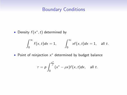
Boundary Conditions
• Density f (x∗, t) determined by
∫
∞
0f (x , t)dx = 1,
∫
∞
0xf (x , t)dx = 1, all t.
• Point of reinjection x∗ determined by budget balance
τ = p
∫ x∗
ρ
0(x∗ − ρx)f (x , t)dx , all t.

Stationary distribution
Proposition
The stationary distribution f (x) has the form
f (x) =
C1x−β1 when x < x∗
C2x−β2 when x > x∗
where β1 < 1 is the smaller root of the characteristic equation
κ2
2β2 −
(
3
2κ2 − (g − g)
)
β + κ2 − p − (g − g) = 0
and β2 > 2 is the larger root of the characteristic equation
κ2
2β2 −
(
3
2κ2 − (g − g)
)
β + κ2 − p − (g − g) + qρβ−1 = 0.

Stationary Distribution, f (x)
See Benhabib and Zhu (2008) for calibration details.

Compare to US Wealth Distribution
-2 -1 0 1 2 3 4 50
0.02
0.04
0.06
0.08
0.1
0.12
Ratio of individual wealth to aggregate wealth
Density
Jess Benhabib Shenghao Zhu (New York University)Age, Luck, and Inheritance January 11, 2008 3 / 29

Simplifications/Limitations
(1) Perpetual Youth
(2) Weird life insurance business
(3) No Labor Income
(4) Stationary distribution only due to government policy
(5) Returns not Persistent
(6) Everything (bequest motive, savings rate etc) homogeneous
• Benhabib, Bisin and Zhu (2011) improves on (1)-(5).

Benhabib, Bisin and Zhu, ECMA (2011)
• Also introduce capital income taxes, estate taxation.
• Samuelson (1965) describing “Pareto’s law”:
In all places and all times, the distribution of income remains
the same. Neither institutional change nor egalitarian taxation
can alter this fundamental constant of social sciences.
• Benhabib, Bisin and Zhu (2011): this is not true. Capital
income and estate taxation can significantly reduce wealth
inequality.

Agent’s Problem
• Agents live for T periods.
• At birth, draw idiosyncratic labor income y(s), and rate of
return on capital r(s), fixed over lifecycle.
• Can be correlated with those of parent.
• Agent’s problem is now
maxC(s,v)
∫ s+T
s
e−ρ(v−s)u(C (s, v))dv + e−ρTφ(W (s, s +T )) s.t
W (s, t) = r(s)W (s, t) + y(s)− C (s, t)
with W (s, s) given.

� �
initial earnings, over dynasties n.

Change of Notation
• More convenient notation:
• keep track of generations n = 0, 1, 2, ...
• use age τ = t − s
maxcn(τ)
∫ T
0u(cn(τ))dτ + e−ρTφ(wn+1(0)) s.t
wn(τ) = rnwn(τ) + yn − cn(τ)
• (rn)n and (yn)n are stochastic processes
• Estate taxation:
wn+1(0) = (1− b)wn(T )

Evolution of Wealth Across Generations
• With CRRA u and φ, get closed form solution for savings. See
Appendix A.
• Can obtain wealth at death given wealth at birth
wn(T ) = σw (rn,T )wn(0) + σy (rn,T )yn
where σw and σy depend on parameters only.
• Let wn = wn(0)
• Recall wn+1 = (1− b)wn(T ).
• Get a stochastic difference equation
wn+1 = α(rn)wn + β(rn, yn)

Stationary Wealth Distribution
• Can analyze this difference equation
• With β(rn, yn) = 0 this would be a random growth process.
• With β(rn, yn) > 0 this is called a Kesten process
• Theorem 1: stationary distribution of initial wealth, wn, has
a Pareto tail
Pr(wn > w) ∼ kw−µ
• Intuition: labor income β(rn, yn) works as lower bound.
• Theorem 2: Stationary distribution of wealth (of all
households of all ages from 0 to T ) also has a Pareto tail with
same exponent µ.

Capital Income and Estate Taxation
• Introduce capital income tax ζ. Let post-tax return be
(1− ζ)rn.
• Proposition 3: The tail index µ increases (i.e. inequality
decreases) with the estate tax b and the capital income tax ζ.
• Can also examine non-linear taxes (1− ζ(rn))rn.
• Corollary 1: The tail index µ increases (i.e. inequality
decreases) with the imposition of a nonlinear tax on capital
ζ(rn).
• Capital income and estate taxes reduce wealth inequality by
reducing capital income risk, not the average return.

Calibration
• Match US Lorenz curve
• Parameterize rn = (.08, .12, .15, .32) and
Pr(rn+1|rn) =
.8 + εlow .12− εlow3 .07− εlow
3 0.01 − εlow3
.8 .12 .07 0.01
.8 .12 .07 0.01
.8−εhigh3 .12−
εhigh3 .07 −
εhigh3 0.01 + εhigh
• εlow controls persistence of lowest rate of return.
• εhigh controls persistence of highest rate of return.
• “frictions to social mobility”

Calibration
TABLE II
PERCENTILES OF THE TOP TAIL; εlow = :01
Percentiles
Economy 90th–95th 95th–99th 99th–100th
United States :113 :231 :347εhigh = 0 :118 :204 :261εhigh = :01 :116 :202 :275εhigh = :02 :105 :182 :341εhigh = :05 :087 :151 :457

Calibration
TABLE III
TAIL INDEX, GINI, AND QUINTILES; εlow = :01
Quintiles
Economy Tail Index µ Gini First Second Third Fourth Fifth
United States 1:49 :803 −:003 :013 :05 :122 :817εhigh = 0 1:796 :646 :033 :058 :08 :123 :707εhigh = :01 1:256 :655 :032 :056 :078 :12 :714εhigh = :02 1:038 :685 :029 :051 :071 :11 :739εhigh = :05 :716 :742 :024 :042 :058 :09 :786

Calibration
TABLE IX
TAX EXPERIMENTS—TAIL INDEX µ
b\ζ 0 :05 :15 :2
0 :68 :76 :994 1:177
:1 :689 :772 1:014 1:205
:2 :7 :785 1:038 1:238
:25 :706 :793 1:051 1:257
TABLE X
TAX EXPERIMENTS—GINI
b\ζ 0 :05 :15 :2
0 .779 .769 .695 .674
:1 .768 .730 .693 .677
:2 .778 .724 .679 .674
:3 .754 .726 .680 .677

Cagetti and De Nardi (2006)
• Benhabib, Bisin and Zhu (2011,2012): stochastic processes
for rate of return on capital exogenously given.
• Cagetti and De Nardi (2006) endogenize this a bit more:
entrepreneurship
• Also embed in general equilibrium

Cagetti and De Nardi (2006)
• Construct a quantitative model consistent with observed data.
• Evaluate model along dimensions not matched by construction
• Study effects of borrowing constraints on aggregates and
wealth inequality
• Results:
• Model accounts very well for wealth distributions of
entrepreneurs and workers
• Model generates entry into entrepreneurship consistent with
estimates
• Model generates entrepreneurial returns consistent with data
• More stringent borrowing constraints ⇒ less inequality but
also less investment
• Voluntary bequests important for wealth concentration

Cagetti and De Nardi (2006)
• Model features:
• Two sectors: entrepreneurial and non-entrepreneurial. All
action is in former.
• Individuals heterogeneous in wealth, working ability and
entrepreneurial ability.
• Occupational choice
• Entrepreneurs operate span of control (i.e. decreasing returns)
technology, face borrowing constraints (limited commitment).
• Next few slides: match of wealth distribution

Model Without Entpreneurs
Fig. 1.—Distribution of wealth, conditional on wealth being positive, for the wholepopulation. Dash-dot line: data; solid line: model without entrepreneurs.

Model With Entrepreneurs
Fig. 2.—Distribution of wealth, conditional on wealth being positive, for the wholepopulation. Dash-dot line: data; solid line: baseline model with entrepreneurs.

Workers vs. Entrepreneurs
Fig. 3.—Distribution of wealth, conditional on wealth being positive, in the baselinemodel with entrepreneurs. Solid line: workers; dash-dot line: entrepreneurs.

Wealth Distribution of Entrepreneurs Only
Fig. 4.—Distribution of the entrepreneurs’ wealth, conditional on wealth being positive.Dash-dot line: data; solid line: baseline model.

Firm Size Distribution
Fig. 6.—Firm size distribution, baseline model with entrepreneurs

Other Related Literature
• Acemoglu (2002), “Technical Change, Inequality, and the
Labor Market”
• Huggett, Ventura and Yaron (2011), “Sources of Lifetime
Inequality”
• Katz and Murphy (1992), “Changes in Relative Wages,
1963-87: Supply and Demand Factors”
• Krueger, Perri, Pistaferri and Violante (2010),
“Cross-Sectional Facts for Macroeconomists”
This is a RED special issue see
http://www.economicdynamics.org/RED-cross-sectional-facts.htm
• Quadrini (1999), “The Importance of Entrepreneurship for
Wealth Concentration and Mobility”
• Quadrini (2000), “Entrepreneurship, Saving and Social
Mobility”