lecture 6: nonstationari.ty error correction modelsatoroj/econometric_methods/lecture_6_ecm.pdf ·...

Stationarity and nonstationarity Testing for integration Cointegration Error correction model

Lecture 6: Nonstationarity. Error Correction Models

Econometric Methods � Warsaw School of Economics

Andrzej Torój

Andrzej Torój

(6) Nonstationarity. ECM 1 / 32


Outline

1 Stationarity and nonstationarity

Notion of stationarity

Random walk as nonstationary time series

2 Testing for integration

Dickey-Fuller test

Augmented D-F speci�cation

3 Cointegration

4 Error correction model

Andrzej Torój



Outline



3 Cointegration


Andrzej Torój




Time series � de�nition

Yt � random variable � takes values with some probabilities(described by density function f (y)/ distribution functionF (y))

values + probabilities: distribution of a random variable

{Yt} � stochastic process � sequence of random variables Yt

ordered by time

{yt} � time series � draw from a stochastic process in one sample

Key parameters of random variable's distribution:

Expected value: E(Y ) =´ +∞−∞ yf (y) dy

Variance: D2(Y ) = E(Y − E(Y ))2

Andrzej Torój




Stationarity

Type I (in the strict sense / strong)

Distribution of the stochastic process is time-invariant (in everyperiod, yt is a value taken by identically distributed random variableYt)

Type II (in the large sense / weak)

� mean and variance constant overtimeE(Yt) = µ <∞D2(Yt) = σ2 <∞� covariance between variables depends on their distance in time(not the moment in time)Cov(Yt ,Yt+h) = Cov(Yt+k ,Yt+k+h) = γ(h)

Andrzej Torój




�White noise�

�White noise� � de�nition

E(εt) = 0 [�uctuations around zero]D2(εt) = σ2 <∞ [homoskedasticity]Cov(εt , εt+h) = 0, h 6= 0 [no serial correlation]

...like the disturbances in the classical linear regression model.

εt ∼ IID(0, σ2)

I � independent

I � indentically

D � distributed

Andrzej Torój




Stationary series � �white noise�

Andrzej Torój




Nonstationary process � �random walk�

Random walk � de�nition

yt = yt−1 + εtyt = yt−1 + εt = yt−2 + εt−1 + εt = yt−3 + εt−2 + εt−1 + εt = . . . =

y0 +∑T

t=1 εty0=0=

T∑t=1

εt︸︷︷︸stochastic trend

Properties of random walk:

E(yt) = E(∑T

t=1 εt) =∑T

t=1 E(εt) = 0

D2(yt) = D2(∑T

t=1 εt)cov(εt ,εt−h)=0

=∑T

t=1 D2(εt) = Tσ2

cov(yt , yt−h) = E(yt , yt−h)− E(yt)E(yt−h) =

E(∑T−h

t=1 εt∑T−h

t=1 εt)−E(

T−h∑t=1

)︸︷︷︸0

E(

T−h∑t=1

)︸︷︷︸0

= D2(∑T−h

t=1 εt) =∑T−h

t=1 D2(εt) = (T−h)σ2

Andrzej Torój




Nonstationary series � random walk

Andrzej Torój




Integration order

Stationary variable is called integrated of order 0, notation: I(0).

Integration order � de�nition

Variable yt is integrated of order d (yt ∼ I (d)) if it can betransformed into a stationary variable after di�erencing d times.

E.g. variable yt generated by the process yt = yt−1 + εt isintegrated of order 1 (yt ∼ I (1)), as yt − yt−1 = εt , and εt ∼ I (0)by de�nition.

First di�erences: ∆yt = yt − yt−1

Second di�erences:∆∆yt = ∆yt−∆yt−1 = yt−yt−1−yt−1+yt−2 = yt−2yt−1+yt−2

(��lter (1,-2,1)�)

Andrzej Torój




Nonstationary process � random walk with drift

Random walk with drift � de�nition

yt = α0 + yt−1 + εtyt = α0 + yt−1 + εt = α0 + α0 + yt−2 + εt−1 + εt =

α0 + α0 + α0 + yt−3 + εt−2 + εt−1 + εt = . . .y0=0= Tα0 +

T∑t=1

εt︸︷︷︸stochastic trend

Random walk with drift � properties:

E(yt) = E(Tα0 +∑T

t=1 εt) = Tα0 +∑T

t=1 E(εt) = Tα0

Variance and covariance � the same as in the case of random walk (adding a constantdoes not a�ect the dispersion).

Andrzej Torój




Nonstationary variable � random walk with drift

Andrzej Torój




Order of integration � why it matters

possible problems:

regression I(1) vs I(1) � spurious regression (trendingvariables)regression I(0) vs I(1) � nonstationary residuals

(economically unlikely), mistakes in statistical inference

(test statistic for variable signi�cance is not t-distributed)

solutions:

transformation of the series (di�erencing, logarithm)respeci�cation of the model (for consistency with the theory)error correction and cointegration

Andrzej Torój



Outline



3 Cointegration


Andrzej Torój



Dickey-Fuller test

Dickey-Fuller (DF)

Dickey and Fuller, 1979, 1981

yt = α1yt−1 + εt

process is stationary if α1 < 1

process is nonstationary if α1 = 1 (then random walk)

H0 : α1 = 1

H1 : α1 < 1

true H0 → nonstationary variables → bias in OLS →hypothesis not veri�able immediately

Andrzej Torój



Dickey-Fuller test

DF � test statistic

Subtract yt−1 from both sides � potentially stationary dependentvariable:

∆yt = (α1 − 1)︸︷︷︸ yt−1 + εt

δ

H0 : δ = 0⇐⇒ α1 = 1⇐⇒ yt ∼ I (1)

H1 : δ < 0⇐⇒ α1 < 1⇐⇒ yt ∼ I (0)

DF emp = δSδ∼ DF

(computed as t-statistic, but with di�erent distribution � seeMacKinnon (1996) )

If DF emp < DF ∗, reject H0 against H1 and consider the processstationary.

Andrzej Torój



Dickey-Fuller test

DF � algorithm

H0 not rejected:

nonstationarity, but unknown order of integration (1 orhigher)...

Test again...

variable is integrated of order 2 (yt ∼ I (2)), if stationary afterdouble di�erentiation

∆(∆yt) = δ∆yt−1 + εt

H0 : δ = 0⇐⇒ yt ∼ I (2)

H1 : δ < 0⇐⇒ yt ∼ I (1)


Andrzej Torój



Dickey-Fuller test

DF � I(2) series

If again H0 not rejected:

variable integrated of order 2 or not rejecting H0 due to lowpower of the test...

Test again...

∆3yt = δ∆2yt−1 + εt

H0 : δ = 0⇐⇒ yt ∼ I (3)

H1 : δ < 0⇐⇒ yt ∼ I (2)


failure to reject the null again � too weak power of the test(too rarely rejects false null hypothesis)

in economics, series integrated of order higher than 2 generallyabsent

Andrzej Torój




Augmented DF

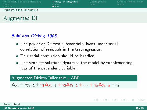
Said and Dickey, 1985

The power of DF test substantially lower under serialcorrelation of residuals in the test regression.

This serial correlation should be handled.

The simplest solution: dynamise the model by supplementinglags of the dependent variable.

Augmented Dickey-Fuller test � ADF

∆yt = δyt−1 + γ1∆yt−1 + γ2∆yt−2 + . . .+ γk∆yt−k + εt

Andrzej Torój




ADF � how many lags?

in general: the purpose is to eliminate the serial correlation ofthe error term

CAUTION! we do not use DW statistic to evaluate it(remember why...?)

auxiliary algorithms: set the maximum lag length to considerand...

...pick the best regression by means of information criteria(AIC, SIC, HQC)...see if the last signi�cant; if not, remove it and check again

rule-of-thumb formula for maximum lag length:(4 · T

100

) 14 ,

where T � sample size (Schwert, 2002)

Andrzej Torój




ADF � speci�cation of test regression

∆yt = δyt−1

(+

k∑i=1

γ i∆yt−i

)+ εt

possible extensions:

∆yt = β + δyt−1 +

(k∑

i=1γ i∆yt−i

)+ εt

→ H0: nonstationary process with drift

additionally: linear trend, quadratic trend, seasonal dummies...

Andrzej Torój




(A)DF � trendstationarity

∆yt = β + δyt−1 +

(k∑

i=1γ i∆yt−i

)+ εt

extension:

∆yt = β + δyt−1 +

(k∑

i=1γ i∆yt−i

)+ γt + εt

→ if H0 rejected and trend t signi�cant � trendstationary series(then include t in the regression)

→ if H0 not rejected, series is nonstationary

Beware the di�erence!

stationary process 6= deterministic trend 6= stochastic trend

Andrzej Torój




Exercise (1)

Test the order of integration of the following variables with ADFtest:� log real wages� log labour productivity� unemployment

Andrzej Torój



Outline



3 Cointegration


Andrzej Torój



Cointegration

Nonstationarity � what then?

dealing with models based on nonstationary variables:

OLS: spurious regressionexplosive behaviour of dynamic modelsI(0)+I(1): nonstationary residuals + false statistical inference

solution: di�erencing I(1) data

OLS, dynamic models: adequate toolsLONG-TERM RELATIONSHIPS lost from the data

Andrzej Torój



Cointegration

Cointegration of time series

dependencies between nonstationary variables � sometimesstable in time...then called COINTEGRATING RELATIONSHIPS

there is a mechanism that brings the system back toequilibrium everytime it is shocked away from it (Grangertheorem)

Cointegration

Time series y1 and y2 are cointegrated (of order d , b), if they are integrated oforder d and there exists their linear combination integrated of order d − b:y1, y2 ∼ CI (d , b)⇐⇒ y1 ∼ I (d) ∧ y2 ∼ I (d) ∧ ∃β 6=0 y

Tβ︸︷︷︸y1β1+y2β2

∼ I (d − b)

Usually: variables integrated of order 1, their combination �

stationary.

Andrzej Torój



Cointegration

Testing for cointegration: Engle-Granger procedure

1 Test the order of integration.

2 If all of them, say, I(1), specify the cointegrating relationship:y1t = β0 + β1y2t + εt

1 estimate parameters β0, β1 via OLS2 compute the residual series (εt)

3 Test these residuals for stationarity � if stationary, variables arecointegrated.

Andrzej Torój



Outline



3 Cointegration


Andrzej Torój



ECM

Error correction model (1)

some �error correction� mechanism directly implied by theGranger theorem

recall the ADL(1,1) model:yt = α0 + α1yt−1 + β0xt + β1xt−1 + εtyt = α0 + α1yt−1 + β0xt + β1xt−1 +εt +yt−1 − yt−1 + xt−1 − xt−1 + β0xt−1 − β0xt−1 + α1xt−1 − α1xt−1

rearranging terms, we obtain the error correction model:

∆yt = (α1 − 1)(yt−1 −α0

1− α1− β0 + β1

1− α1xt−1︸︷︷︸

ECT : ˆεt−1

) + β0∆xt + εt

Andrzej Torój



ECM

Error correction model (2)

Procedure:

1 estimate the cointegrating relationship

2 estimate the ECM, using di�erenced variables and laggedresiduals from the cointegrating relationship

variables are cointegrated when (α1 − 1) < 0

> 0: disequilibrium expands= 0: no error correction(−1; 0): error correction (close to 0: slow, close to -1: quick;

half − life = ln(0.5)ln(α1)

)

= −1: full error correction in 1 period< −1: overshooting, oscillatory adjustment

Andrzej Torój



ECM

Exercise (2)

Consider the following variables:� log real wages (dependent)� log labour productivity� unemploymentWhat is their order of integration?Are they cointegrated?Are the signs in the cointegrating relationship economically rea-sonable?Is there error correction mechanism at work?What is the half-life of the adjustment?Example inspired by Zasova, Melihovs (2005)

Andrzej Torój


http://www.bank.lv/public_files/images/img_lb/izdevumi/english/citas/Labour_market.pdf


ECM

Readings

Greene:

Chapter 20 � Models With Lagged VariablesChapter 21 - Time-Series ModelsChapter 22 - Nonstationary Data

Andrzej Torój


lecture 6: nonstationari.ty error correction modelsatoroj/econometric_methods/lecture_6_ecm.pdf ·...

Documents