lecture 6 competition, monopoly, monopolistic...
TRANSCRIPT

Lecture 6Competition, Monopoly, Monopolistic
Competition and Oligopoly
1
Overview
Firm supply decisions in a perfectly competitive market– Short run supply– Long run supply
Competitive equilibriumMonopoly
– Supply decisions– Barriers to entry/sources of monopoly power
Monopolistic Competition
2

Overview
Oligopoly– Rivals reactions– Nash equilibrium– Prisoners’ Dilemma
Measuring market structure
3
Market structure
Start by looking at extreme cases– Competitive market
• Many firms• Commodity market obvious example
– Monopoly markets• Single seller• Firm with patent, government protection or access
to scarce resource
4

Market structure
Intermediate Cases– Monopolistic competition
• Many firms• Firms sell differentiated products• Some market power
– Oligopolistic markets• Few sellers• Barriers to entry
– Take into account rivals response to your actions
5

Competitive or Commodity Markets
Characteristics of a Commodity Market
1. Price taking
2. Product homogeneity
3. Free entry and exit
4. Perfect Information
6
Commodity Markets
Price Taking
– The individual firm sells a very small share of the total market output
• Cannot influence market price
• Firm’s demand curve is perfectly elastic
– The individual consumer buys too small a share of industry output to have any impact on market price.
– Examples: wheat farmer, me buying gas.7
Commodity Markets
Product Homogeneity
– The products of all firms are perfect substitutes
– Small differences in quality
– Examples
• Agricultural products, oil, copper, iron, lumber, coal
8
Characteristics of Substitutes
Two products tend to be close substitutes when– They have similar performance characteristics– They have similar occasion for use and– They are sold in the same geographic area
9
Commodity Markets
Free Entry and Exit
– Buyers can easily switch from one supplier to another
– Suppliers can easily enter or exit a market– All factors of production are perfectly mobile
in the long-run
10
Commodity Markets
Perfect Information– Every consumer knows about all goods being
produced and their prices– All producers have well defined production
functions– Can relax these assumptions
11
Commodity Markets
Do we believe these assumptions hold all the time? – Seem to hold in commodity markets– Other markets have characteristics similar to
commodity marketsEven if all the conditions do not hold,
competition can still be fierce if at least two hold– Predictions of basic model will still hold
12
Perfectly Competitive Markets
Need to be aware of the assumptions so that we know whether the assumptions are violated in such a way that the model is no longer validWe will talk about other market structures
where some of these assumptions don’t hold
13

Profit Maximizing Choice of Output
Determining the profit maximizing level of output– Profit (π ) = Total Revenue - Total Cost– Total Revenue (R) = Pq– Total Cost (C) = Cq– Therefore:
)()()( qCqRq −=π
14

Profit Maximizing Choice of Output
0
Cost,Revenue,
Profit($s per year)
Output (units per year)
R(q)Total Revenue
Slope of R(q) = MR
15
Profit Maximizing Choice of Output
0
Cost,Revenue,
Profit($s per year)
Output (units per year)
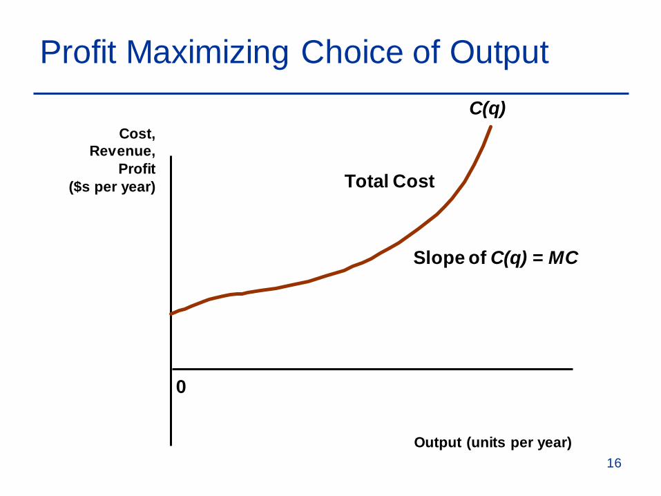
C(q)
Total Cost
Slope of C(q) = MC
16

Profit Maximizing Choice of Output
0
Cost,Revenue,
Profit($s per year)
Output (units per year)
R(q)
C(q)
q*
Distance between the two curves is π.
17
Profit Maximizing Choice of Output
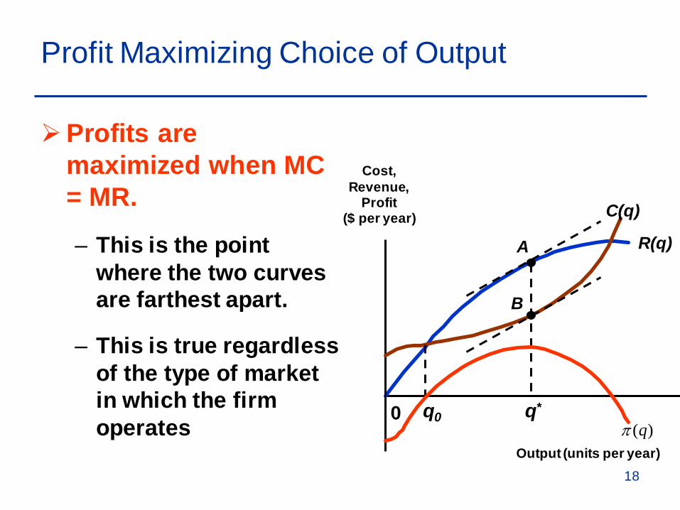
Profits are maximized when MC = MR.
– This is the point where the two curves are farthest apart.
– This is true regardless of the type of market in which the firm operates
R(q)
0
Cost,Revenue,
Profit($ per year)
Output (units per year)
C(q)
A
B
q0 q*
)(qπ
18

Marginal Revenue, Marginal Cost, and Profit Maximization
C - R =πqR MR
∆∆
=
qCMC∆∆
=
19

Marginal Revenue, Marginal Cost, and Profit Maximization
orqC
qR 0
q
: whenmaximized are Profits
=∆∆
−∆∆
=∆∆π
MC(q)MR(q)MCMR=
=− thatso0
20
Profit Maximizing Choice of Output
Consider the case for a firm operating in a commodity market.– The firm is a price taker.– Revenue is given by: R(q)=P*q. – MR=P and R(q) is a horizontal line.
Call market output (Q), and firm output (q). market demand (D) and firm demand (d).
21

Demand and Marginal Revenue Facedby a Competitive Firm
Output (bushels)
Price$ per bushel
Price$ per bushel
Output (millions of bushels)
d$4
100 200 100
Firm Industry
D
$4
22
The Competitive Firm’s Demand
Profit Maximization occurs where: MC(q) = MR = P.
Let’s combine production and cost analysis to see again why this is the profit maximizing (or cost minimizing) point for the firm to produce.
23

q0 q1 q2
A Competitive Firm Making a Positive Profit
10
20
30
40
Price($ perunit)
0 1 2 3 4 5 6 7 8 9 10 11
50
60MC
AVC
ATCAR=MR=P
Outputq*
At q*: MR = MCand P > ATC
ABCDorqx AC) -(P *= π
D
BC
A
24
A Competitive Firm Making a Positive Profit
The way I have drawn these curves P>AVC and P>ATC.Firm is making a profit.However, in the short-run firm will produce
as long as P>AVC, even if P<AFC.Why?Let’s see why.
25

A Competitive Firm Incurring LossesPrice($ perunit)
Output
AVC
ATCMC
q*
P = MR
B
F
C
A
E
DAt q*: MR = MCand P < ATCLosses = (P- AC) x q*
or ABCD
If firm produced 0 then losses=CBFE or amount of fixed costs
26

Price($ per
unit)
MC
Output
AVC
ATC
P = AVC
P1
P2
q1 q2
S = MC above AVC
A Firm’s Short-Run Supply Curve
Shut-down
27

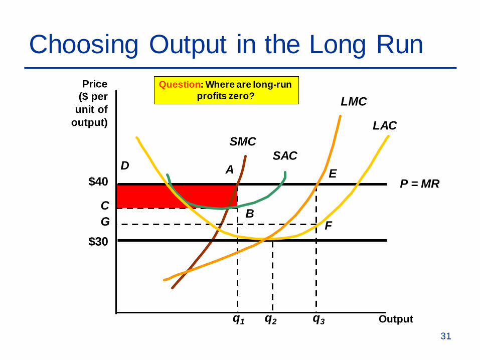
Choosing Output in the Long Run
In the long run, a firm can alter all its inputs, including the amount of machinery and the size of the plant.
Firms can also enter and exit the industry at no cost.
28

Choosing Output in the Long Run
Firms continue to use the same rule when choosing output; P=MC.However, now the relevant marginal cost
is long-run marginal cost.Firms produce output as long as P ≥LRAC
29

Choosing Output in the Long Run
Recall that we have assumed that firms can enter the industry at no cost and begin producing output.What will firms do if they see an industry
where firms are earning a positive profit?– Note, this is above the opportunity cost for all
of the resources being employed.Firms will enter the industry until long-run
profits are zero.
30
q1
A
BC
D
Choosing Output in the Long RunPrice
($ perunit of
output)
Output
P = MR$40
SACSMC
Question: Where are long-run profits zero?
q3q2
G F$30
LAC
E
LMC
31
S1
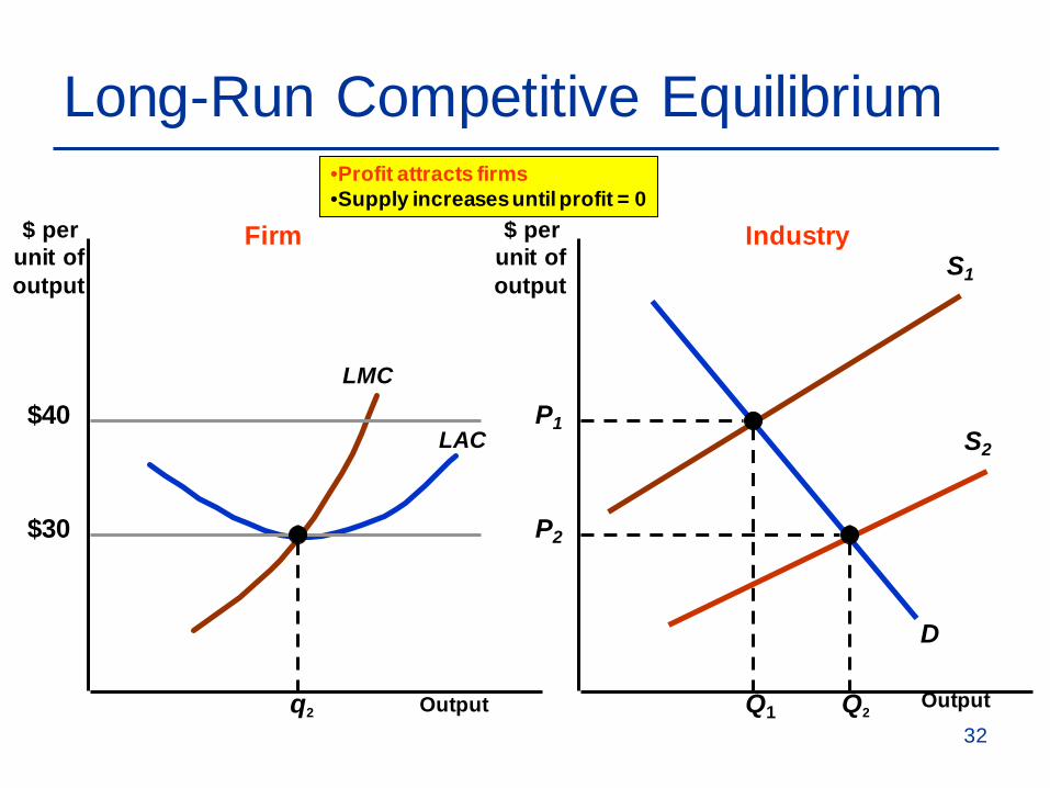
Long-Run Competitive Equilibrium
Output Output
$ per unit ofoutput
$ per unit ofoutput
$40LAC
LMC
D
S2
P1
Q1q2
Firm Industry
$30
Q2
P2
•Profit attracts firms•Supply increases until profit = 0
32

Choosing Output in the Long Run
Long-Run Competitive Equilibrium
1) MC = MR
2) P = LAC• No incentive to leave or enter
• Profit = 0
3) Equilibrium Market Price—quantity demanded equals quantity supplied.
33

Monopoly
The monopolist is the supply-side of the market and has complete control over the amount offered for sale.
Profits will be maximized at the level of output where marginal revenue equals marginal cost.
34
Monopoly
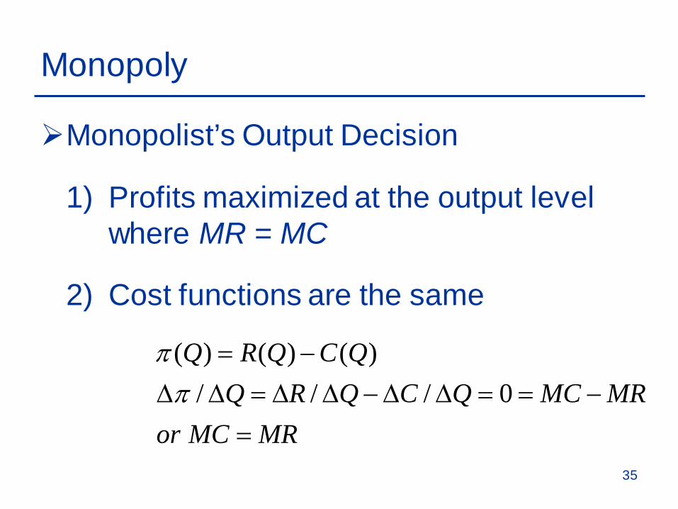
Monopolist’s Output Decision
1) Profits maximized at the output level where MR = MC
2) Cost functions are the same
MRMCorMRMCQCQRQ
QCQRQ
=−==∆∆−∆∆=∆∆
−=0///
)()()(π
π
35
Maximizing Profit When Marginal Revenue Equals Marginal Cost
Moving to output levels below MR = MC the increase in revenue is greater than the increase in cost (MR > MC).Moving to output levels above MR = MC
the increase in cost is greater than the increase in revenue (MR < MC)
The Monopolist’s Output Decision
36

Lostprofit
P1
Q1
Lostprofit
MC
Quantity
€ perunit ofoutput
D = AR
MR
P*
Q*
Maximizing Profit When Marginal Revenue Equals Marginal Cost
P2
Q237
Monopoly
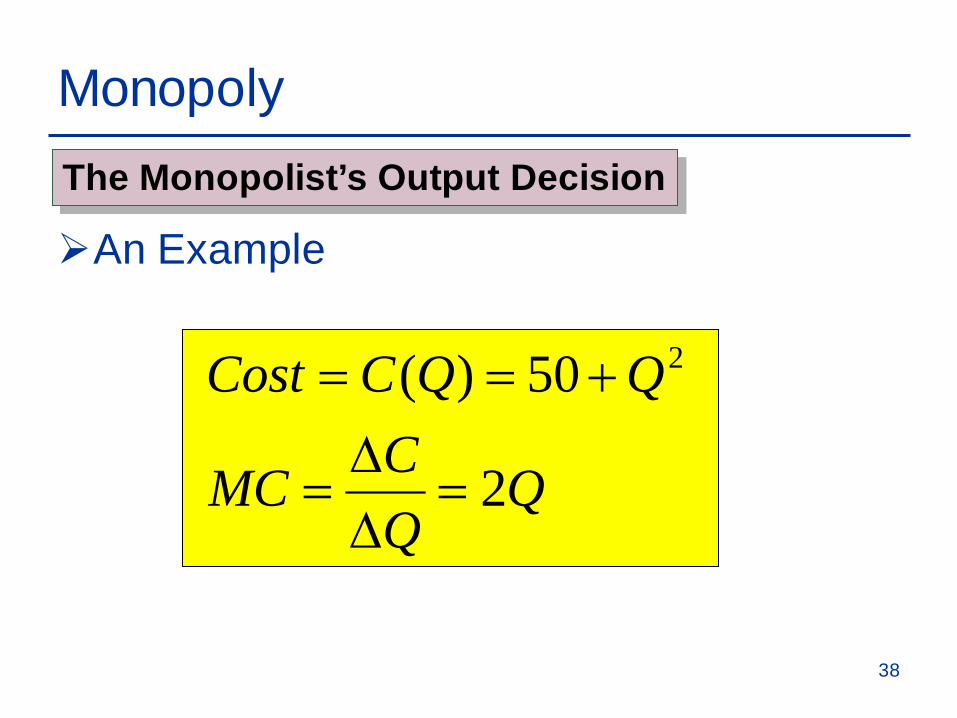
An Example
QQCMC
QQCCost
2
50)( 2
=∆∆
=
+==
The Monopolist’s Output Decision
38
Monopoly
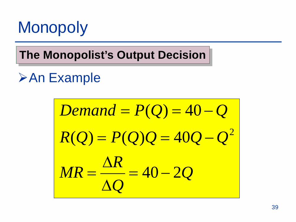
An Example
QQRMR
QQQQPQRQQPDemand
240
40)()(40)(
2
−=∆∆
=
−==
−==
The Monopolist’s Output Decision
39
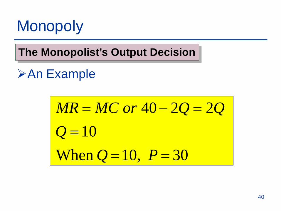
Monopoly
An Example
30 10,When 10
2240
===
=−=
P QQ
QQorMCMR
The Monopolist’s Output Decision
40

Monopoly
An Example– By setting marginal revenue equal to marginal
cost, it can be verified that profit is maximized at P = $30 and Q = 10.
The Monopolist’s Output Decision
41
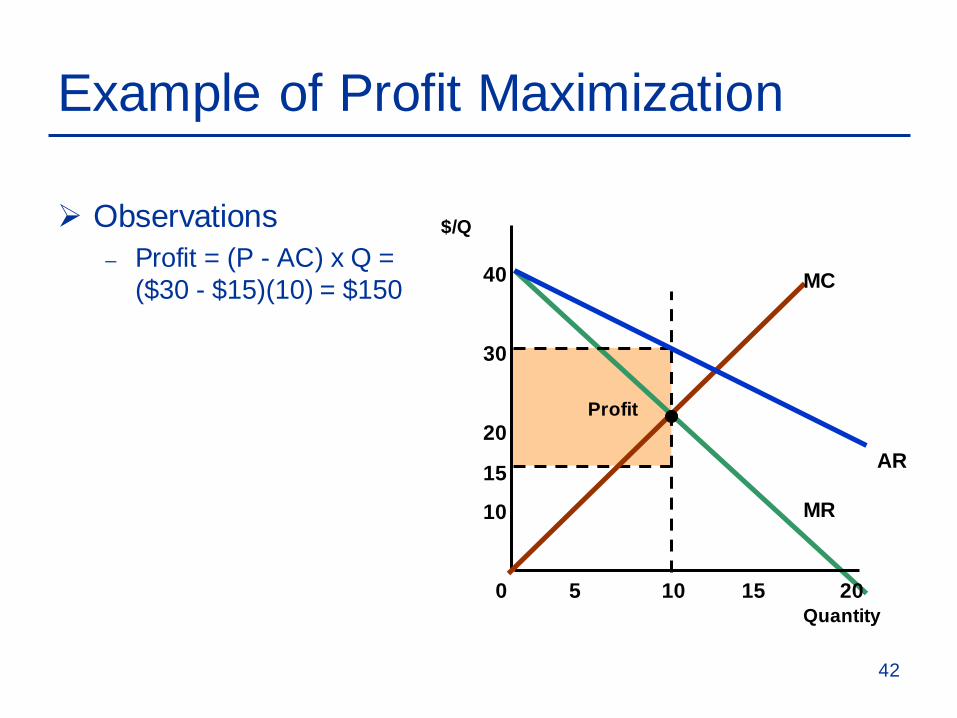
Example of Profit Maximization
Observations– Profit = (P - AC) x Q =
($30 - $15)(10) = $150
Quantity
$/Q
0 5 10 15 20
10
20
30
40
15
MC
AR
MR
Profit
42
Sources of Market Power
A firm’s monopoly power is determined by the firm’s elasticity of demand. – More sensitive demand is to changes in price
the closer we are to the competitive outcome (P=MC).
43

Monopoly
A Rule of Thumb for Pricing– We want to translate the condition that
marginal revenue should equal marginal cost into a rule of thumb that can be more easily applied in practice.
44

A Rule of Thumb for Pricing
Can show that optimal price is:
Where E*D is the elasticity of demand at the optimal level of output. – When demand is perfectly elastic P=MC.
( )*DE11
MCP +
=
45

Sources of Monopoly Power
The firm’s elasticity of demand is determined by:1) Elasticity of market demand2) Number of firms3) The interaction among firms
Anything that limits the number of substitutes for a firm’s product will enhance its market power.
46
Sources of Monopoly Power
Some of the things that limit substitutes are:
1. Control over a unique input or special knowledge—Specific Assets
2. The government Governments frequently limits entry into
markets through the use of licenses and other devices.
47
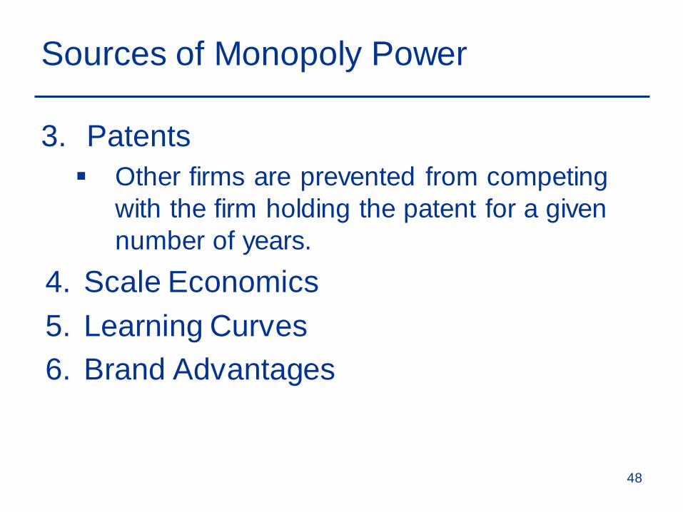
Sources of Monopoly Power
3. Patents Other firms are prevented from competing
with the firm holding the patent for a given number of years.
4. Scale Economics5. Learning Curves6. Brand Advantages
48

The Social Costs of Monopoly Power
Monopoly power results in higher prices and lower quantities.However, does monopoly power make
consumers and producers in the aggregate better or worse off?
49

BA
Lost Consumer Surplus
Deadweight Loss
Because of the higherprice, consumers lose
A+B and producer gains A-C.
C
Deadweight Loss from Monopoly Power
Quantity
AR
MR
MC
QC
PC
Pm
Qm
$/Q
50
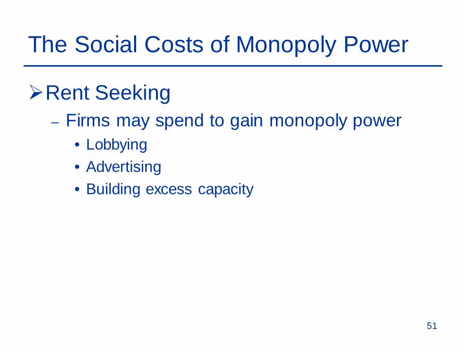
Rent Seeking– Firms may spend to gain monopoly power
• Lobbying• Advertising• Building excess capacity
The Social Costs of Monopoly Power
51
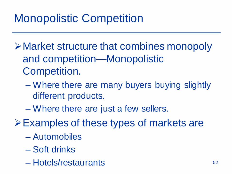
Monopolistic Competition
Market structure that combines monopoly and competition—Monopolistic Competition.– Where there are many buyers buying slightly
different products.– Where there are just a few sellers.
Examples of these types of markets are– Automobiles– Soft drinks– Hotels/restaurants 52
Introduction
Our models for these markets will combine some aspects of the competitive model and some aspects of the monopoly model.
53
Monopolistic Competition
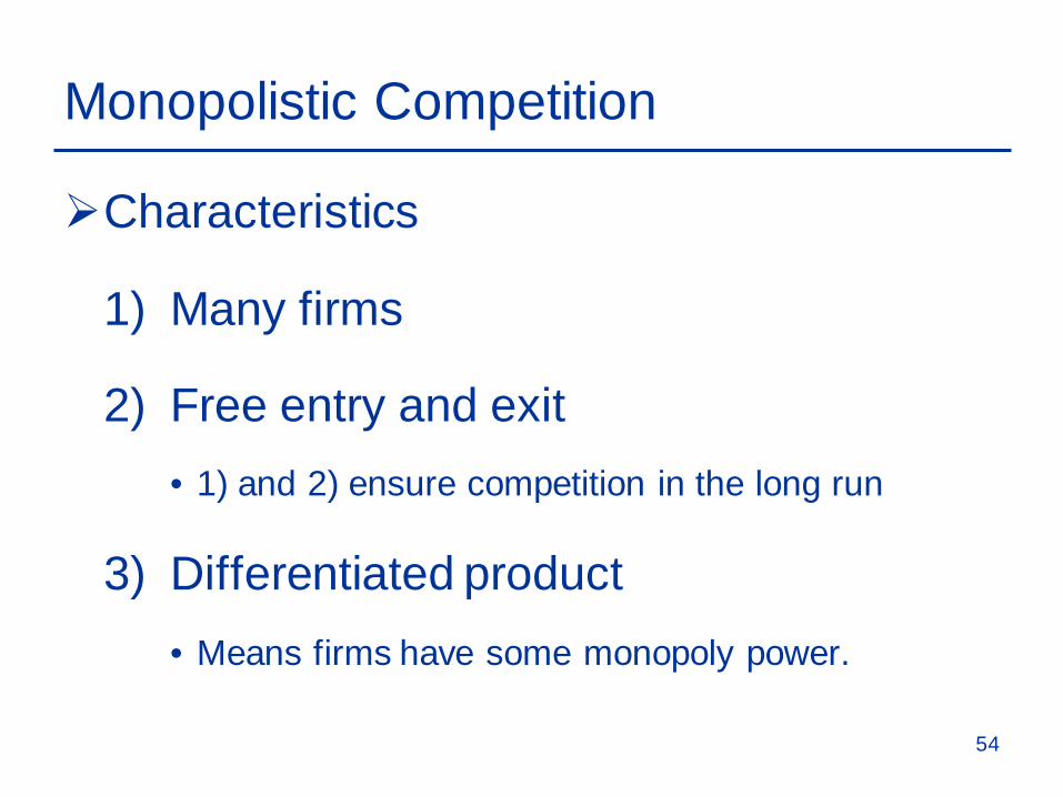
Characteristics
1) Many firms
2) Free entry and exit• 1) and 2) ensure competition in the long run
3) Differentiated product• Means firms have some monopoly power.
54
Monopolistic Competition
The amount of monopoly power depends on the degree of differentiation.
Automobile– Ferrari and monopoly power
• Consumers can have a preference for Ferrari—performance, handling, style
• The greater the preference (differentiation) in consumers’ minds the higher the price.
55

Monopolistic Competition
The Makings of Monopolistic Competition– Two important characteristics
• Differentiated but highly substitutable products• Free entry and exit
56

Monopolistic Competition
How do firms differentiate their products?– Presumably through advertising.– This is actual the origin of this model, trying to
explain advertising.Why do firms want to do this?
57
A Monopolistically CompetitiveFirm in the Short and Long Run
Quantity
$/Q
Quantity
$/QMC
AC
MC
AC
DSR
MRSR
DLR
MRLR
QSR
PSR
QLR
PLR
Short Run Long Run
58

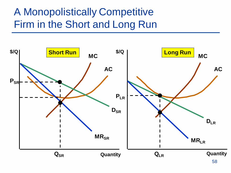
Observations (short-run)– Downward sloping demand--differentiated
product– Demand is relatively elastic--good substitutes– MR < P– Profits are maximized when MR = MC– This firm is making economic profits
A Monopolistically CompetitiveFirm in the Short and Long Run
59
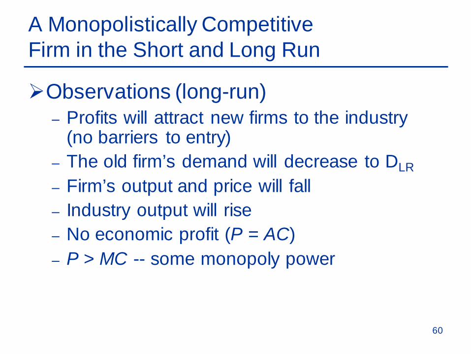
Observations (long-run)– Profits will attract new firms to the industry
(no barriers to entry)– The old firm’s demand will decrease to DLR
– Firm’s output and price will fall– Industry output will rise– No economic profit (P = AC)– P > MC -- some monopoly power
A Monopolistically CompetitiveFirm in the Short and Long Run
60
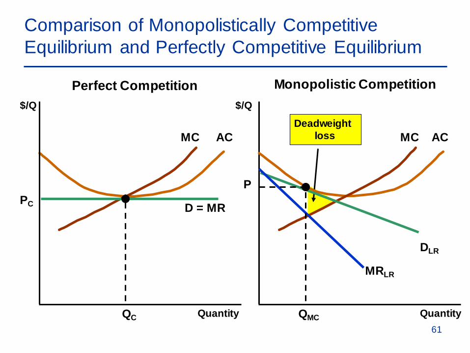
Deadweight lossMC AC
Comparison of Monopolistically CompetitiveEquilibrium and Perfectly Competitive Equilibrium
$/Q
Quantity
$/Q
D = MR
QC
PC
MC AC
DLR
MRLR
QMC
P
Quantity
Perfect Competition Monopolistic Competition
61

Monopolistic Competition
Monopolistic Competition and Economic Efficiency– The monopoly power (differentiation) yields
a higher price than perfect competition. If price was lowered to the point where MC = D, total surplus would increase by the yellow triangle.
62

Monopolistic Competition
Monopolistic Competition and Economic Efficiency– Although there are no economic profits in
the long run, the firm is still not producing at minimum AC and excess capacity exists.
63

Monopolistic Competition Versus Perfect Competition
Monopolistic competition is similar to perfect competition.– Each firm acts independently, without regard
to the responses of its competitors. – Free entry guarantees that firms earn zero
economic profits in the long-run.
64
Monopolistic Competition Versus Perfect Competition
Monopolistic competition differs from perfect competition. – Monopolistic competitors are not price takers. – The firm's equilibrium price exceeds its
marginal cost.– Firms have excess capacity in long-run
equilibrium.
65

Nonprice Competition
Firms in monopolistic competition sometimes engage in nonprice competition. – Provide better-quality products.– Product characteristics are designed to match
the preferences of specific groups of consumers.
– May involve location.
66
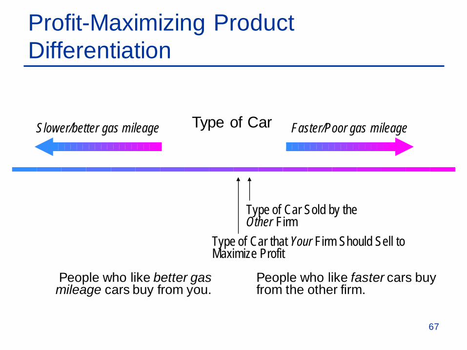
Profit-Maximizing Product Differentiation
People who like better gas mileage cars buy from you.
People who like faster cars buy from the other firm.
Type of Car Sold by the Other Firm
Type of Car that Your Firm Should Sell to Maximize Profit
Type of Car Slower/better gas mileage Faster/Poor gas mileage
67
Oligopoly
Characteristics– Small number of firms– Product differentiation may or may not exist– Barriers to entry
Oligopoly exists in markets where a few producers produce most of the output
68

Ten Most Concentrated IndustriesPercentage of Value of Shipments Accounted for by the Largest Firms in High-Concentration Industries, 1992
SIC NO.
INDUSTRYDESIGNATION
FOURLARGEST
FIRMS
EIGHTLARGEST
FIRMS
NUMBEROF
FIRMS
2823 Cellulosic man-made fiber 98 100 53331 Primary copper 98 99 113633 Household laundry equipment 94 99 102111 Cigarettes 93 100 82082 Malt beverages (beer) 90 98 1603641 Electric lamp bulbs 86 94 762043 Cereal breakfast foods 85 98 423711 Motor vehicles 84 91 3983482 Small arms ammunition 84 95 553632 Household refrigerators and
freezers82 98 52 69
Oligopoly
What are some barriers to entry?– Natural
• Scale economies• Patents• Technology• Name recognition/branding
70
Oligopoly
What are some barriers to entry?
– Strategic action• Flooding the market• Controlling an essential input
71
Oligopoly
Management Challenges– Strategic actions– Rival behavior
Question– What are the possible rival responses to a
10% price cut by Ford?
72
Oligopoly
Equilibrium in an Oligopolistic Market– In perfect competition, monopoly, and
monopolistic competition producers did not have to consider a rival’s response when choosing output and price.
– In oligopoly producers must consider the response of competitors when choosing output and price.
73
Oligopoly
Equilibrium in an Oligopolistic Market– Defining Equilibrium
• Firms do the best they can and have no incentive to change their output or price
• All firms assume competitors are taking rival decisions into account.
74

Oligopoly
Nash Equilibrium– Each firm is doing the best it can given what
its competitors are doing.
75
Oligopoly
The Cournot Model– Duopoly
• Two firms competing with each other. They choose output independently.
• Homogenous good• The output of the other firm is assumed to be fixed• Barriers to new entry
76
MC1
50
MR1(75)
D1(75)
12.5
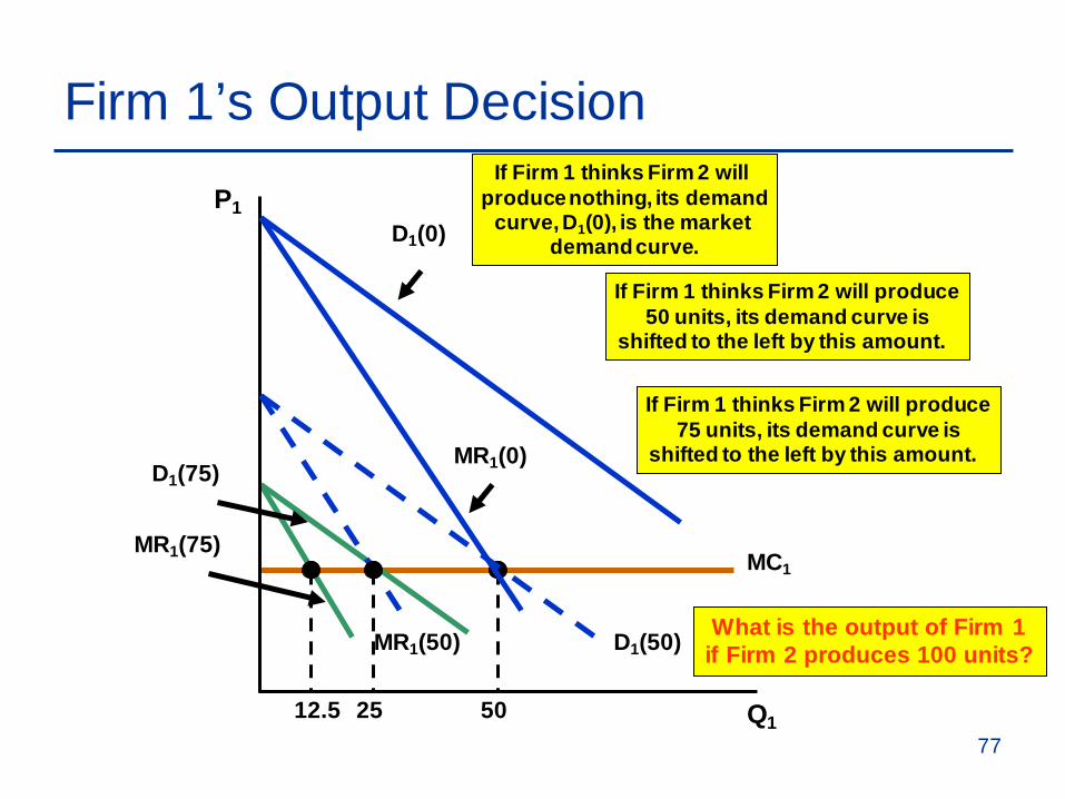
If Firm 1 thinks Firm 2 will produce75 units, its demand curve is
shifted to the left by this amount.
Firm 1’s Output Decision
Q1
P1
What is the output of Firm 1if Firm 2 produces 100 units?
D1(0)
MR1(0)
If Firm 1 thinks Firm 2 will produce nothing, its demand
curve, D1(0), is the market demand curve.
D1(50)MR1(50)
25
If Firm 1 thinks Firm 2 will produce50 units, its demand curve is
shifted to the left by this amount.
77
Oligopoly
The Reaction Curve– A firm’s profit-maximizing output is a
decreasing function of the expected output of Firm 2.
78
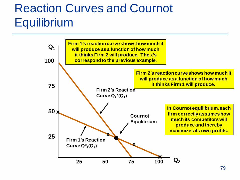
Firm 2’s ReactionCurve Q2*(Q1)
Firm 2’s reaction curve shows how much itwill produce as a function of how much
it thinks Firm 1 will produce.
Reaction Curves and Cournot Equilibrium
Q2
Q1
25 50 75 100
25
50
75
100
Firm 1’s ReactionCurve Q*1(Q2)
x
xx
x
Firm 1’s reaction curve shows how much itwill produce as a function of how much
it thinks Firm 2 will produce. The x’s correspond to the previous example.
In Cournot equilibrium, eachfirm correctly assumes how
much its competitors willproduce and thereby
maximizes its own profits.
CournotEquilibrium
79
Oligopoly
An Example of the Cournot Equilibrium– Duopoly
• Market demand is P = 30 - Q where Q = Q1 + Q2
• MC1 = MC2 = 0
The Linear Demand Curve
80
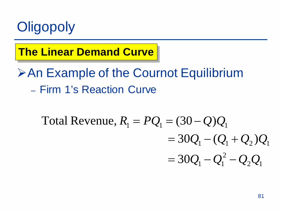
Oligopoly
An Example of the Cournot Equilibrium– Firm 1’s Reaction Curve
111 )30( Revenue, Total QQPQR −==
122
11
1211
30
)(30
QQQQQQQQ
−−=
+−=
The Linear Demand Curve
81
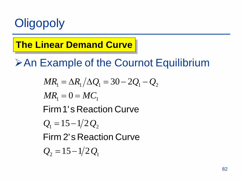
Oligopoly
An Example of the Cournot Equilibrium
12
21
11
21111
2115
2115
0230
MCMRQQQRMR
−=
−=
==−−=∆∆=
Curve Reaction s2' Firm
Curve Reaction s1' Firm
The Linear Demand Curve
82
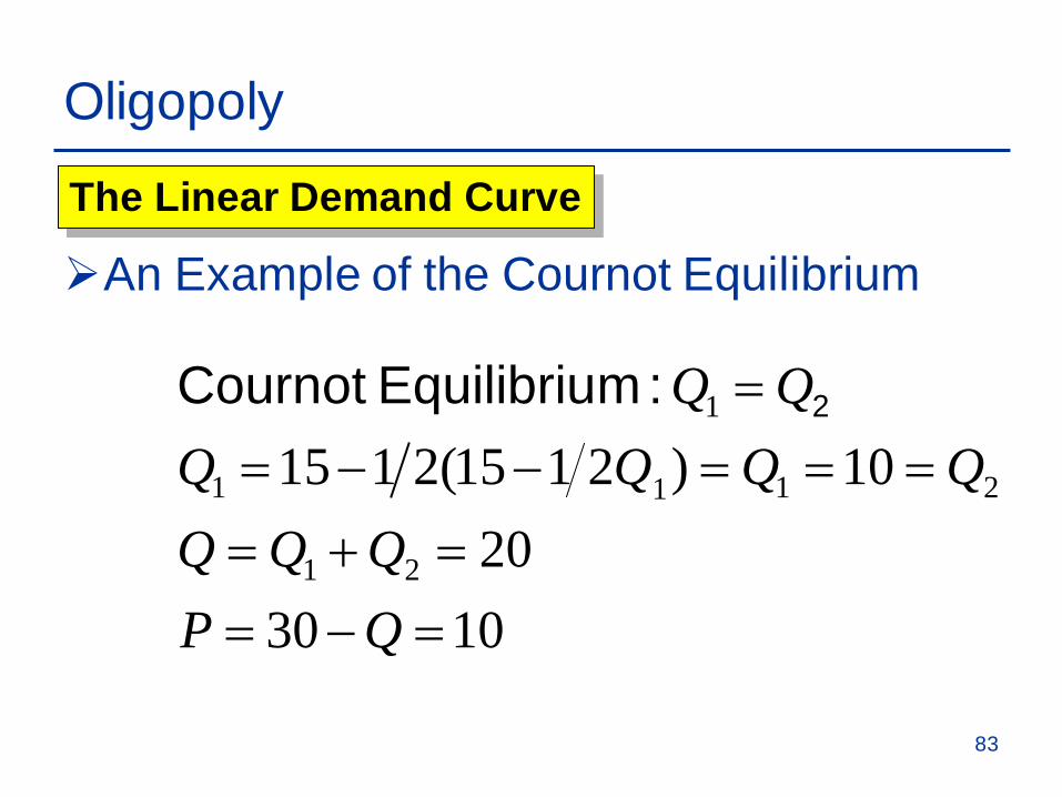
Oligopoly
An Example of the Cournot Equilibrium
103020
10)2115(2115
21
2111
1
=−==+=
===−−==
QPQQQ
QQQQQQ 2:mEquilibriu Cournot
The Linear Demand Curve
83
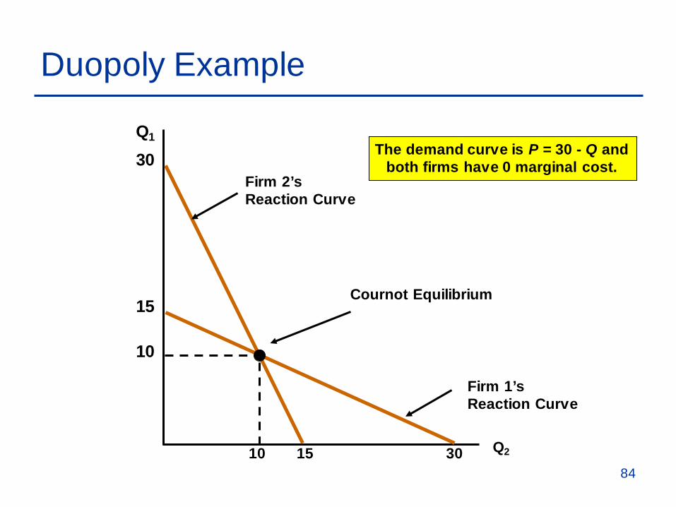
Duopoly Example
Q1
Q2
Firm 2’sReaction Curve
30
15
Firm 1’sReaction Curve
15
30
10
10
Cournot Equilibrium
The demand curve is P = 30 - Q andboth firms have 0 marginal cost.
84
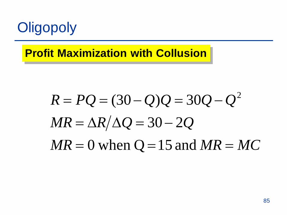
Oligopoly
MCMRMRQQRMR
QQQQPQR
===−=∆∆=
−=−==
and 15 Q when 0230
30)30( 2
Profit Maximization with Collusion
85
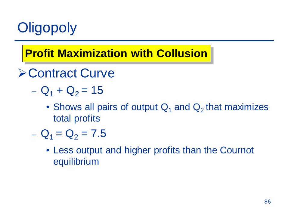
Oligopoly
Contract Curve– Q1 + Q2 = 15
• Shows all pairs of output Q1 and Q2 that maximizes total profits
– Q1 = Q2 = 7.5• Less output and higher profits than the Cournot
equilibrium
Profit Maximization with Collusion
86
Firm 1’sReaction Curve
Firm 2’sReaction Curve
Duopoly Example
Q1
Q2
30
30
10
10
Cournot Equilibrium15
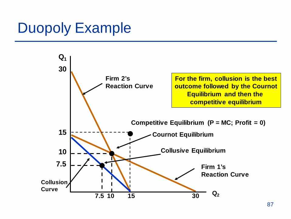
15
Competitive Equilibrium (P = MC; Profit = 0)
CollusionCurve
7.5
7.5
Collusive Equilibrium
For the firm, collusion is the bestoutcome followed by the Cournot
Equilibrium and then the competitive equilibrium
87
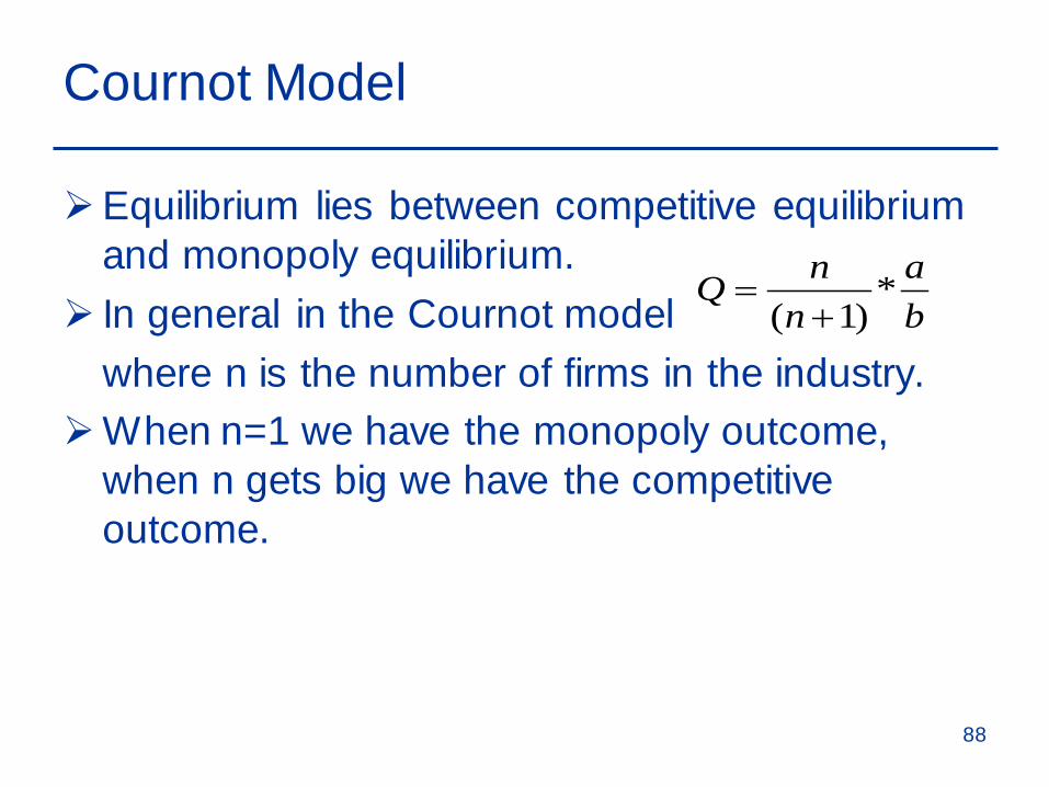
Cournot Model
Equilibrium lies between competitive equilibrium and monopoly equilibrium.
In general in the Cournot model where n is the number of firms in the industry.
When n=1 we have the monopoly outcome, when n gets big we have the competitive outcome.
*( 1)
n aQn b
=+
88
First Mover Advantage-- The Stackelberg Model
Assumptions– One firm can set output first– MC = 0– Market demand is P = 30 - Q where Q = total
output– Firm 1 sets output first and Firm 2 then makes
an output decision
89

Firm 1– Must consider the reaction of Firm 2
Firm 2– Takes Firm 1’s output as fixed and therefore
determines output with the Cournot reaction curve: Q2 = 15 - 1/2Q1
First Mover Advantage-- The Stackelberg Model
90

Firm 1
– Choose Q1 so that:
122
1111 300
Q - Q - QQ PQ R MC, MC MR
==
=== 0 MR therefore
First Mover Advantage--The Stackelberg Model
91

Substituting Firm 2’s Reaction Curve for Q2:
5.7 and 15:015
21
1111
===−=∆∆=QQMRQQRMR
211
112
111
2115
)2115(30
QQQQQQR
−=
−−−=
First Mover Advantage--The Stackelberg Model
92

Conclusion– Firm 1’s output is twice as large as firm 2’s– Firm 1’s profit is twice as large as firm 2’s
Questions– Why is it more profitable to be the first mover?– Which model (Cournot or Stackelberg) is more
appropriate?
First Mover Advantage--The Stackelberg Model
93
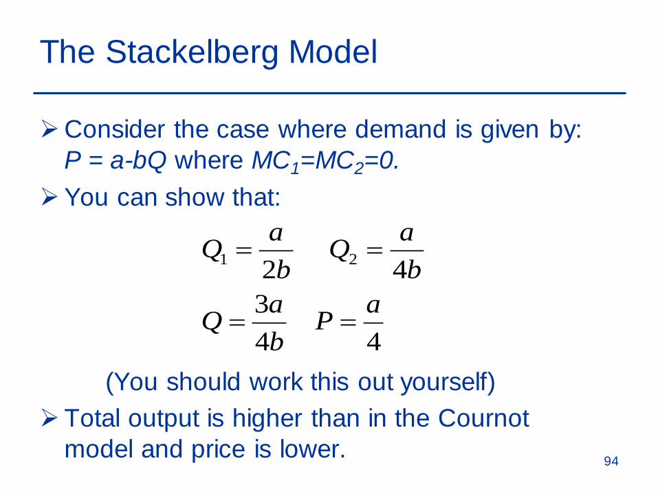
The Stackelberg Model
Consider the case where demand is given by: P = a-bQ where MC1=MC2=0.
You can show that:
(You should work this out yourself)Total output is higher than in the Cournot
model and price is lower.
1 22 434 4
a aQ Qb b
a aQ Pb
= =
= =
94
Price Competition
Competition in an oligopolistic industry may occur with price instead of output.
The Bertrand Model is used to illustrate price competition in an oligopolistic industry with homogenous goods.
95
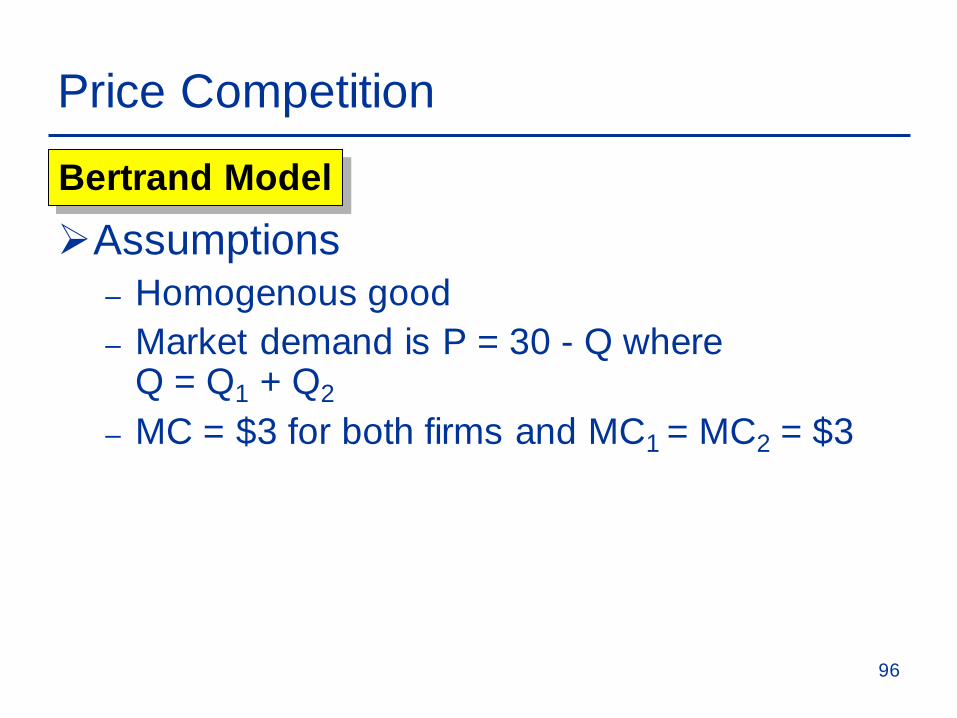
Price Competition
Assumptions– Homogenous good– Market demand is P = 30 - Q where
Q = Q1 + Q2
– MC = $3 for both firms and MC1 = MC2 = $3
Bertrand Model
96

Price Competition
Assumptions– The Cournot equilibrium:
– Now, assume the firms compete with price, not quantity.
Bertrand Model
$81 firms both for
====
π912$ 21 QQP
97

Price Competition
How will consumers respond to a price differential? (Hint: Consider homogeneity)– The Nash equilibrium:
• P = MC; P1 = P2 = $3• Q = 27; Q1 & Q2 = 13.5•
Bertrand Model
0=π
98
Price Competition
Why not charge a higher price to raise profits?
How does the Bertrand outcome compare to the Cournot outcome?
The Bertrand model demonstrates the importance of the strategic variable (price versus output).
Bertrand Model
99
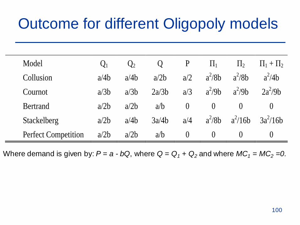
Outcome for different Oligopoly models
Model Q1 Q2 Q P Π1 Π2 Π1 + Π2 Collusion a/4b a/4b a/2b a/2 a2/8b a2/8b a2/4b Cournot a/3b a/3b 2a/3b a/3 a2/9b a2/9b 2a2/9b Bertrand a/2b a/2b a/b 0 0 0 0 Stackelberg a/2b a/4b 3a/4b a/4 a2/8b a2/16b 3a2/16b Perfect Competition a/2b a/2b a/b 0 0 0 0
Where demand is given by: P = a - bQ, where Q = Q1 + Q2 and where MC1 = MC2 =0.
100
Competition Versus Collusion:The Prisoners’ Dilemma
Each firms profits are highest when they collude
Why wouldn’t each firm set the collusion price independently and earn the higher profits that occur with explicit collusion?
101
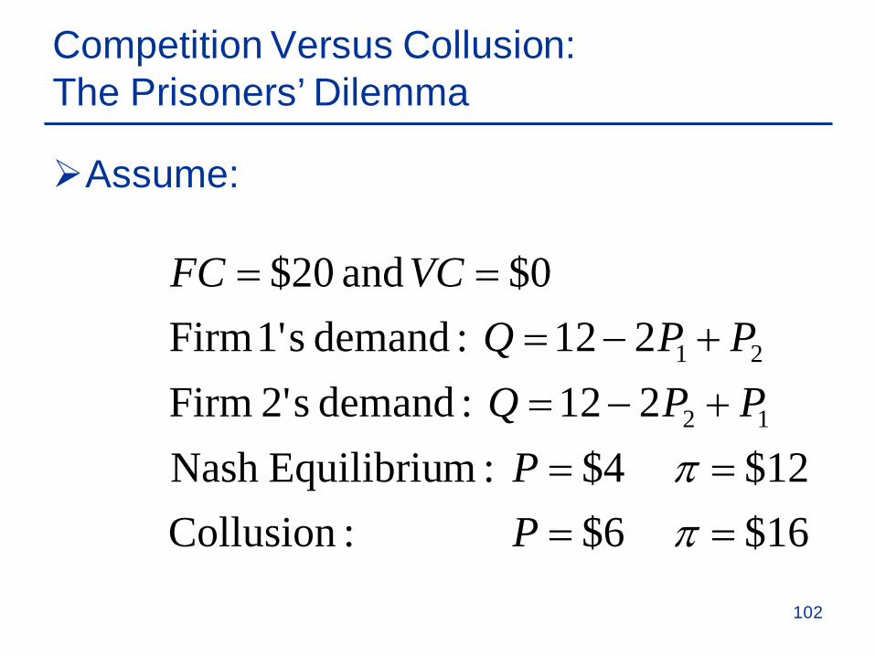
Assume:
16$ 6$ :Collusion12$ 4$ :mEquilibriuNash
212 :demand s2' Firm212 :demand s1' Firm
0$ and 20$
12
21
====+−=+−=
==
ππ
PP
PPQPPQ
VCFC
Competition Versus Collusion:The Prisoners’ Dilemma
102
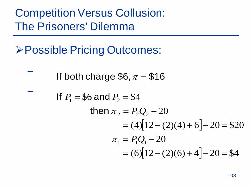
Possible Pricing Outcomes:
–
–$16 $6, charge both If =π
Competition Versus Collusion:The Prisoners’ Dilemma
[ ]
[ ] 4$204)6)(2(12)6(20
20$206)4)(2(12)4(20
4$6$
111
222
21
=−+−=−=
=−+−=−=
==
then and If
QP
QPPP
π
π
103

Payoff Matrix for Pricing Game
Firm 2
Firm 1
Charge $4 Charge $6
Charge $4
Charge $6
$12, $12 $20, $4
$16, $16$4, $20
104

These two firms are playing a noncooperative game.– Each firm independently does the best it can
taking its competitor into account.
Question– Why will both firms both choose $4 when $6
will yield higher profits?
Competition Versus Collusion:The Prisoners’ Dilemma
105

Cartels
Characteristics
1) Explicit agreements to set output and price
2) May not include all firms
106

Cartels
– Examples of successful cartels
• OPEC• International Bauxite
Association• Mercurio Europeo
– Examples of unsuccessful cartels
• Copper• Tin• Coffee• Tea• Cocoa
Characteristics
3) Most often international
107
Cartels
Conditions that make forming a cartel easier.– Potential for monopoly power—inelastic
demand.– A concentrated industry.– Firms compete primarily on price.
108

Cartels
What makes it easier to prevent cheating?– Few firms in the industry– Stable demand– Public prices– Repeated interactions
109
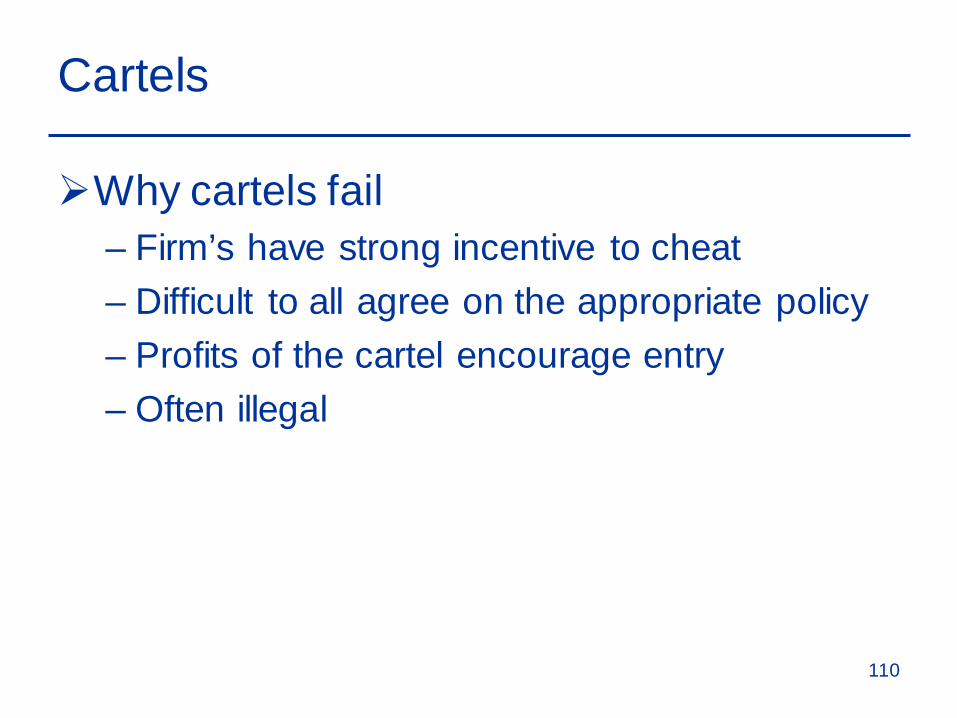
Cartels
Why cartels fail– Firm’s have strong incentive to cheat– Difficult to all agree on the appropriate policy– Profits of the cartel encourage entry– Often illegal
110

Market Structure
Markets are often described by the degree of concentration– Common measure is N-firm concentration
ratio = combined market share of the largest N firms (such as 4 or 20)
– Another is Herfindahl index, the sum of squared market shares
𝐻𝐻𝑖𝑖 = ∑𝑖𝑖(𝑆𝑆𝑖𝑖)2
Where 𝑆𝑆𝑖𝑖 is firm i’s share of output
111

Measuring Market Structure
Monopoly is one extreme with the highest concentration - one sellerPerfect competition is the other extreme
with many, many sellers
112
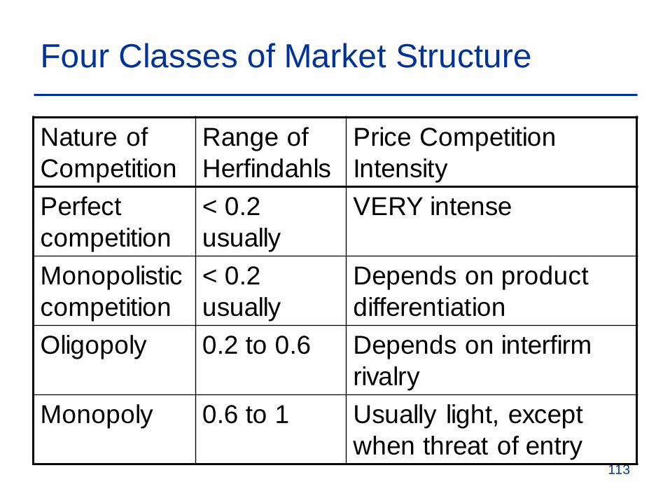
Four Classes of Market Structure
Nature of Competition
Range of Herfindahls
Price Competition Intensity
Perfect competition
< 0.2 usually
VERY intense
Monopolistic competition
< 0.2 usually
Depends on product differentiation
Oligopoly 0.2 to 0.6 Depends on interfirm rivalry
Monopoly 0.6 to 1 Usually light, except when threat of entry
113
Competition Level Varies within Market Structure
A monopoly market may produce the same outcomes as a competitive marketA market with as few as two firms can lead
to fierce competitionWith monopolistic competition, level of
product differentiation determines the intensity of price competitionDo not rely solely on Herfindahl index!!!
114
Summary
We assume that all firms try and maximize profits.
A competitive firm makes its output choice under the assumption that the demand for its own output is horizontal.
115

Summary
In the short run, a competitive firm maximizes its profit by choosing an output at which price is equal to (short-run) marginal cost.
In the long-run, profit-maximizing competitive firms choose the output at which price is equal to long-run marginal cost.
116
Summary
Market power is the ability of sellers or buyers to affect the price of a good.Monopoly power is determined in part by
the number of firms competing in the market.Market power can impose costs on societyIn a monopolistically competitive market,
firms compete by selling differentiated products, which are highly substitutable.
117

Summary
Firms with market power are in an enviable position because they have the potential to earn large profits, but realizing that potential may depend critically on the firm’s pricing strategy.
A pricing strategy aims to enlarge the customer base and capture as much consumer surplus as possible.
118
Summary
In an oligopolistic market, only a few firms account for most or all of production.
In the Cournot model of oligopoly, firms make their output decisions at the same time, each taking the other’s output as fixed.
In the Stackelberg model, one firm sets its output first.
119

Summary
The Nash equilibrium concept can also be applied to markets in which firms produce substitute goods and compete by setting price.
In a cartel, producers explicitly collude in setting prices and output levels.
Firms would earn higher profits by collusively agreeing to raise prices, but the antitrust laws usually prohibit this. 120