lecture 5 advanced (= modern) regression analysis numerical analysis of biological and environmental...
TRANSCRIPT

Lecture 5 Advanced (= Modern) Regression Analysis
NUMERICAL ANALYSIS OF BIOLOGICAL AND
ENVIRONMENTAL DATA
John Birks

Generalised Linear Models (GLM)-What are GLMs?-A simple GLM-Advantages of GLM-Structure of GLM
Error functionLinear predictorLink function
ADVANCED REGRESSION ANALYSIS = MODERN
REGRESSION ANALYSIS
-Parameter estimation-Minimal adequate model-Concept of deviance-Model building-Model notation-Examples of models-Model criticismClassification
Locally weighted regression (LOWESS)Spline functions
Generalised additive models (GAM)Classification and regression trees (CART)
Examples of modern techniquesArtificial neural networks
Software

Brew, J.S. & Maddy, D. 1995. Generalised linear modelling. In Statistical Modelling of Quaternary Science Data (eds. D. Maddy & J.S. Brew) – Quaternary Research Association Technical Guide 5
Crawley, M.J. 1993. GLIM for ecologists – Blackwell
Crawley, M.J. 2002. Statistical computing: An introduction to data analysis using S-PLUS – Wiley
Crawley, M.J. 2005. Statistics. An introduction using R - Wiley
Crosbie, S.F. & Hinch, G.N. 1985. New Zealand J. Agr. Research 28, 19-29
Faraway, J.J. 2004. Linear Models with R. Chapman & Hall/CRC.
Faraway, J.J. 2006. Extending the Linear Model with R – Chapman & Hall/CRC
Fox, J. 2002. An R and S-PLUS companion to applied regression – Sage.
McCullagh, P. & Nelder, J.A. 1989. Generalized Linear Models – Chapman & Hall
Nicholls, A.O. 1989. Biological Conservation 50, 51-75
O’Brian, L. 1992. Introducing Quantitative Geography. Measurement, Methods and Generalized Linear Models - Routledge
GENERALISED LINEAR MODELS

y = a + bx
y = a + bx + cx2 = a + bx + cz (x2 = z)
y = a + bex = a + bz where z = exponential (x)
Some non-linear models can be linearised by transformation
y = exp (a + bx)
Logny = a + bx
Michaelis-Menten equation
Not a straight-line relationship between response variable and predictor variable.
Linear model is an equation that contains mathematical variables, parameters and random variables that is LINEAR in the parameters and the random variables.
bxax
y
1
xba
y11
Take reciprocals
WHAT ARE GENERALISED LINEAR MODELS?

Linear models are not necessarily straight-line models:
a) polynomial (y =1 + x – x2/15)
b) exponential (y = 3 + 0.1ex)
Inverse polynomials:
a) The Michaelis-Menten or Holling functional response equation;
b) The n-shaped curve 1/y = a + bx + c/x
These are linear models!

Some models are intrinsically non-linear:
xcb
ay
cxbeay 1
hyperbolic function
asymptotic exponential
No transformation can linearise them in all parameters

EXAMPLES OF GENERALISED LINEAR FUNCTIONS

Want to find linear combinations of predictor (= explanatory or independent) (x) variables which best predict the response variable (y).
Five steps:
1. Identification of response (y) and predictor (x) variables.
2. Identification of model equation.
3. Choice of appropriate error function for response variable.
4. Appropriate model parameter estimation procedures.
5. Appropriate model evaluation procedures.
Primary aim - provide a mathematical expression for use in description, interpretation, prediction, or reconstruction involving the relationship between variables y = a + bx
A SIMPLE GENERALISED LINEAR MODEL
bxayInfluences estimates of a and bSystematic
Errorcomponent component
R

ADVANTAGES OF GLM
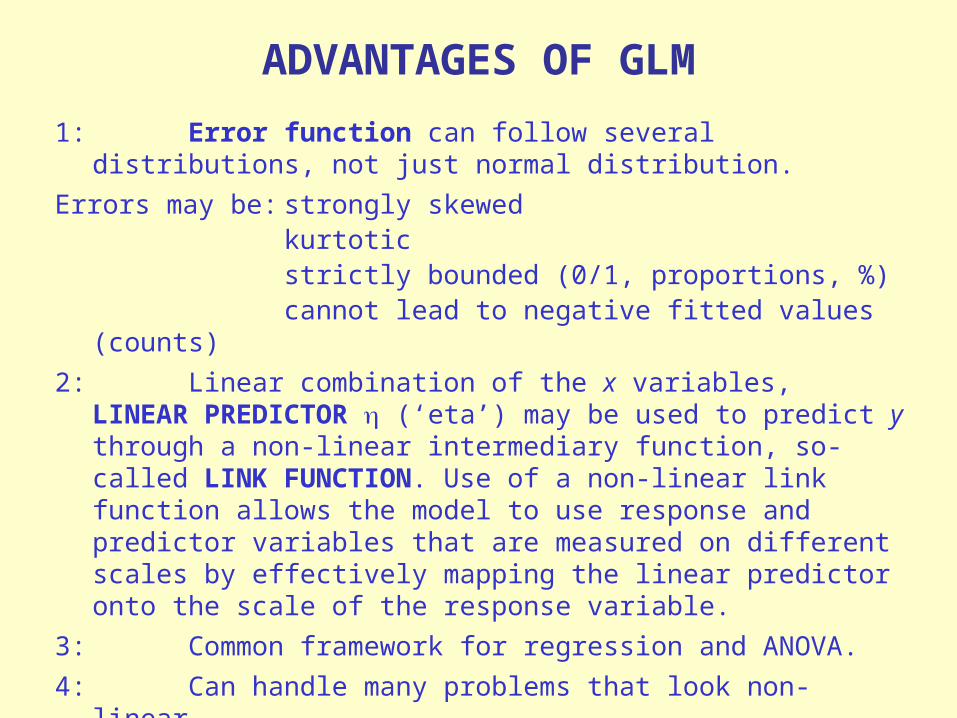
1: Error function can follow several distributions, not just normal distribution.
Errors may be: strongly skewedkurtoticstrictly bounded (0/1, proportions, %)cannot lead to negative fitted values (counts)
2: Linear combination of the x variables, LINEAR PREDICTOR (‘eta’) may be used to predict y through a non-linear intermediary function, so-called LINK FUNCTION. Use of a non-linear link function allows the model to use response and predictor variables that are measured on different scales by effectively mapping the linear predictor onto the scale of the response variable.
3: Common framework for regression and ANOVA.
4: Can handle many problems that look non-linear.
5: Not necessary to transform data since the regression is transformed through the link function.

STRUCTURE OF GENERALISED LINEAR MODEL(1)ERROR FUNCTION
Poisson count dataBinomial proportions, 1/0Gamma data with constant coefficient of variationExponential data on time to death (survival analysis)
CHARACTERISTICS OF COMMON GLM PROBABILITY DISTRIBUTIONS
Choice depends on range of y and on the proportional relationship between variance and expected value .
Probability Range of yVariance function
Gaussian - to 1
Poisson 0 (1)
Binomial 0 (1) n (1 - /)
Gamma 0 to 2
Inverse Gaussian
0 to 3

Some members of the exponential family of probability distributions

ECOLOGICALLY MEANINGFUL ERROR DISTRIBUTIONS
J. Oksanen (2002)
Normal errors rarely adequate in ecology, but GLM offer ecologically meaningful alternatives.
•Poisson. Counts: integers, non-negative, variance increases with mean.
•Binomial. Observed proportions from a total: integers, non-negative, have a maximum value, variance largest at = 0.5.
•Gamma. Concentrations: non-negative real values, standard deviation increases with mean, many near-zero values and some high peaks.

(2) LINEAR PREDICTOR
unknown parameters
predictor variables
LINEAR STRUCTUREj
m
j
ijx
1
To determine fit of a given model, linear predictor is needed for each value of response variable and then compares predicted value with a transformed value of y, the transformation to be applied specified by LINK FUNCTION. The fitted value is computed by applying the inverse of the link function to get back to the original scale of measurement of y.
Log-link - Fitted values are anti-log of linear predictor
Reciprocal link - Fitted values are reciprocal of linear predictor

(3) LINK FUNCTION
Link function relates the mean value of y to its linear predictor (η). η = g(μ)where g(·) is link function and μ are fitted values of y.
Linear predictor is sum of terms for each of the parameters and value of is obtained by transforming value of y by link function and obtaining predicted value of y as inverse link function.
μ = g-1(η)
Can combine link function and linear predictor to form basic or core equation of GLM. Error
component
Linear predictorLink function
OR
y = g-1 (η) + ε
g(y) = η + ε
y = predictable component + error component
y = +

Symbol Link function Formula Use
I Identity η = μRegression or ANOVA with normal errors
L Log η = log μCount data with Poission errors
G Logit η = log zProportion data
with binomial errors
R Reciprocal η = Continuous data
with gamma errors
P Probit η = Φ-1(μ/n)Proportion data in
bioassays
CComplementary
log-logη = log[–log(1-μ/n)
Proportion data in dilution assays
S Square root η = √μ Count dataE Exponent η = μ** number Power functions
The link functions used by GLIM. The canonical link function for normal errorsis the identity link, for Poission errors the log link, for binomial errors the logitlink and for gamma errors the reciprocal link.
-n
1
Some common link functions in generalised linear modelsLink GLIM notation
($LINK=)Link function
(η=)IdentityLogarithmicLogitProbit
ILGP
μlog μ
log (μ/n –μ)
Φ-1 (μ/n)√μ
μ**{number}1/μ
Notes: the following are defaut configurations set automatically by GLIM if $LINKis omitted:
Square rootExponentReciprocal
SER
NormalPoissonBinomialGamma Reciprocal
Error Implied $LINK
IdentityLogarithmicLogit
ENSURE FITTED VALUES STAY
WITHIN REASONABLE
BOUNDS
Link Function Definition Range of fitted valueIdentity η = μ -∞ to ∞
Log η = ln μ 0 to ∞Power p η = μP 0 to ∞
Logit η = ln[μ/(1- μ)] 0 to 1Probit η = Φ-1(μ) 0 to 1
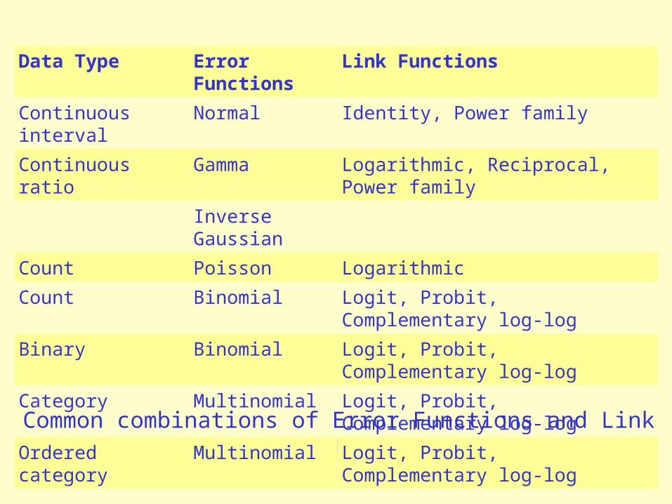
Common combinations of Error Functions and Link Functions
Data Type Error Functions
Link Functions
Continuous interval
Normal Identity, Power family
Continuous ratio Gamma Logarithmic, Reciprocal, Power family
Inverse Gaussian
Count Poisson Logarithmic
Count Binomial Logit, Probit, Complementary log-log
Binary Binomial Logit, Probit, Complementary log-log
Category Multinomial Logit, Probit, Complementary log-log
Ordered category Multinomial Logit, Probit, Complementary log-log

Linkfunction
Regression Continuous Continuous Identity NormalANOVA Continuous Factor Identity NormalANCOVA Continuous Both continuous Log Gamma
and factorRegression Continuous Continuous Reciprocal GammaContingency Count Factor Log PoissontableProportions Proportion Continuous Logit BinomialProbit Proportion Continuous Probit Binomial
(dose)Survival Binary Factor Complementary Binomial
(alive or dead) log-logSurvival Time to death Continuous Reciprocal Exponential
Examples of some error distributions and link functionsType of analysis Response
variableExplanatory
variableError
distribution
Method Link function Error distributionLinear regression Identity NormalANOVA Identity NormalANOVA (random effects) Identity GammaLog-linear model: symmetric Poisson Logarithmic asymmetric Binomial or Multinomial Logit
Binomial or multinomialLogit regression Binomial or multinomial Logit
Probit regression Probit
Examples of generalised linear models
Source: After O’Brian (1983) and O’Brian and Wrigley (1984)
TYPES OF GLM ANALYSIS

GENERALISED LINEAR MODELS – A SUMMARY
Mathematical extensions of linear models that do not force data into unnatural scales. Thereby allow for non-linearity and non-constant variance structures in the data.
Based on an assumed relationship (link function) between the mean of the response variable and the linear combination of the predictor variables.
Data can be assumed to be from several families of probability distributions – normal, binomial, Poisson, gamma, etc – which better fit the non-normal error structures of most real-life data.
More flexible and better suited for analysing real-life data than 'conventional' regression techniques.

Given error function and link function can now formulate linear predictor term. Need to be able to estimate its parameters and find linear predictor that minimises the deviance.
Normal distribution, least-squares algorithm appropriate. Other error functions need maximum likelihood estimation.
In maximum likelihood, aim is find parameter values that give ‘best fit’ to the data. Best in ML considers:
1. data on response variable y2. model specification3. parameter estimates
Need to find the MINIMAL ADEQUATE MODEL to describe the data.
‘BEST’ model is that producing the minimal residual deviance subject to the constraint that all the parameters in the model are statistically significant.
Model should be minimal because of principle of parsimony and adequate because there is no point in retaining an inadequate model that does not describe a significant part of the variation in the data.
NO ONE MODEL, many possible models may be adequate. Need to find MINIMAL ADEQUATE MODEL.
PARAMETER ESTIMATION

1. Models should have as few parameters as possible.
2. Linear models are to be preferred to non-linear models.
3. Models relying on few assumptions are to be preferred to models with many assumptions.
4. Models should be simplified until they are minimal adequate.
5. Simple explanations are to be preferred to complex ones.
Maximum likelihood estimation, given the data, model, link, and error functions, provides values for the parameters by finding iteratively the parameter values in the model that would make the data most likely, i.e. to find the parameter values that maximise the likelihood of the data being observed.
Depends not only on the data but on the model specification.
PRINCIPLE OF PARSIMONY (Ockham’s Razor)

Deviance - measure of the goodness of fit
Fitted values are most unlikely to match the observed data perfectly. Size of discrepancy between model and data is a measure of the inadequacy of the model. DEVIANCE is measure of discrepancy. Twice the log likelihood of the observed data under a specified model.
Its value is defined relative to an arbitrary constant, so that only differences in DEVIANCE (i.e. ratios of likelihoods) have any useful meaning.
CONSTANT is deviance for FULL MODEL – parameter for each observation – is zero.
Discrepancy of fit is proportional to twice the difference between the maximum log likelihood achievable and that attained using a particular model.
OTHER OUTPUT FOR GLM
Parameter estimates, standard errors, t-valuesStandardised parameter estimates (estimates/se)Fitted valuesCovariance matrix for parameter estimatesStandardised residuals
CONCEPT OF DEVIANCE

The formulae used by GLIM in calculating deviance, where y is the data and μ is the fitted value under the model in question (the grand mean in the simplest case); note that, for the grand mean, the term Σ(y – μ) = 0 in the Poisson deviance, and so this reduces to 2Σyln(y/μ); in the binomial deviance, n is the sample size (the binomial denominator), out of which y successes were obtained.
CALCULATION OF DEVIANCE
Error structure Deviance
Normal (y - )2
Poisson 2[y ln (y/) – (y - )]
Binomial 2{y ln (y/) + (n – y) ln [(n – y)/(n - )]}
Gamma 2[-ln (y/) + (y - )/]
Inverse Gaussian (y - )2/(2y)
REF
REF
REF
REF

Aim is to find minimal adequate model and use deviance as principal criterion for assessing different models.
GENERAL LINEAR MODELS• Common framework for Regression Analysis and ANOVA
• Goodness of fit: Sum of Squares (SS)
• Least squares estimation
• Degrees of freedom (df) = {Number of observations} minus {number of parameters}, or df = n – p
• Statistical testing: Compare two models with different number (p and m) of estimated parameters
mpdiff SSSSSS mpdfdfdf mpdiff
diffmp SS2
pnSS
dfSSF
p
diffdiffpnmp /
/,
MODEL BUILDING

Is the regression coefficient significant?
μ = b0
df = N – 1SS0
μ = b0 + b1x
df = N – 2SSA
2
10
21 NSS
SSF
AN /
/SS - A
,
REGRESSION ANALYSIS

ANOVA (Analysis of variance)
Are the class means equal?
AABB
CC
μ = b0
df = N – 1SS0
μ = b0 + b1B +
b2C
df = N – 3SSA
CLASS
A B C
1 1 0 0
2 0 1 0
3 0 0 1
3
10
32 NSS
SSF
AN /
/SS - A
,

In GLM we have DEVIANCE RATIO TEST To consider if model A is a significant improvement over model B, we use:
BB
BABA
dfDdfdfDD
F//
Bdf
df
B/ Deviancedifference )/difference (Deviance
Value greater than tabulated value of F would indicate model A is a significant improvement over model B.
F corresponding to =0.05 df1 = dfA – dfB
df2 = dfB

i
log LL 22
2 22
πσ - σ
- μx ii
Least squares maximize Normal log-likelihood
Other error distributions can be used in analogous way
Deviance is based on log-likelihood, and has the same distribution- Deviance = 0: Observed and fitted values are equal (=
‘deviation’)- Deviance is always positive
Log-likelihood, Sum of Squares and Deviance follow Chi-Squared distribution
Scaled Chi-Squared distribution follows F distribution
LEAST SQUARES AND MAXIMUM LIKELIHOOD
REF
REF
REF
REF

Deviance: Same distribution as Sum of Squares - Chi-squared: Model fits
- F test: Scaled deviance Tests exactly like general linear models Expected value of deviance = degrees of freedom Overdispersion: Model does not fit
- Deviance > degrees of freedom Deviance must be scaled
- Divide by overdispersion coefficient (D/df)- Use F test (scaling automatic)
STATISTICAL TESTING IN GLM

GOODNESS OF FIT AND MODEL INFERENCE
J. Oksanen (2002)
• Deviance: Measure of goodness of fit
– Derived from the error function: Residual sum of squares in Normal error
– Distributed approximately like x2
• Residual degrees of freedom: Each fitted parameter uses one degree of freedom and (probably) reduces the deviance.
• Inference: Compare change in deviance against change in degrees of freedom
• Overdispersion: Deviance larger than expected under strict likelihood model
• Use F–statistic in place of x2.

The aim of the exercise is to determine the minimal adequate model in which all the parameters are significantly different from zero. This is achieved by a step-wise process of model simplification, beginning with the full model, then proceeding by the elimination of non-significant terms, and the retention of significant terms.
One parameter for each and every data pointFit: perfectDegrees of freedom: noneExplanatory power of model: noneContains all (p ) factors, interactions and covariates that might be of interestMany of the model’s terms may be insignificantDegrees of freedom: n – p – 1A simplified model with termsAll the terms are significant (if there are no significant terms, then MAM = null model)Degrees of freedom: n – p’ – 1
Explanatory power: r 2 = SSR/SSTA single parameter, the grand meanFit: noneDegrees of freedom: n – 1Explanatory power of model: none
Full model
Maximal model
Minimal adequate model
Null model
pp 10
MODEL BUILDING
MINIMAL ADEQUATE MODEL
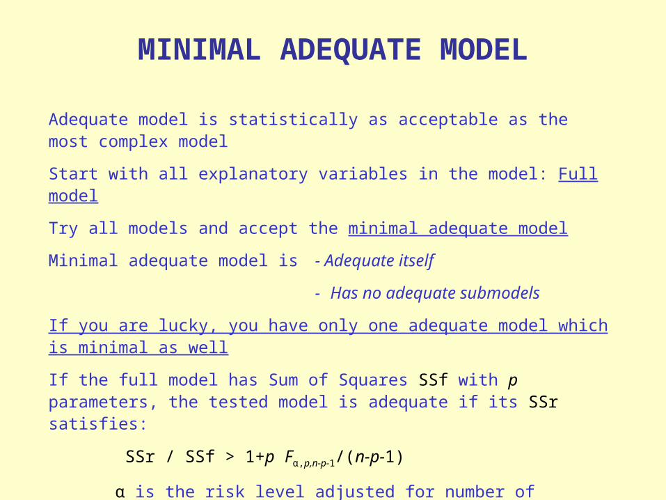
Adequate model is statistically as acceptable as the most complex model
Start with all explanatory variables in the model: Full model
Try all models and accept the minimal adequate model
Minimal adequate model is - Adequate itself
- Has no adequate submodels
If you are lucky, you have only one adequate model which is minimal as well
If the full model has Sum of Squares SSf with p parameters, the tested model is adequate if its SSr satisfies:
SSr / SSf > 1+p Fα,p,n-p-1/(n-p-1)
α is the risk level adjusted for number of parameters,
e.g. α = 1-0.05p

The steps involved in model simplification. There are no hard and fast rules, and this is only a guide to one sensible way of approaching the problem of model simplification.
Step Procedure Explanation1 Fit the maximal model Fit all the factors, interactions and covariates of
interest. Note the residual deviance. Check for overdispersion (Poisson or binomial errors), and rescale if necessary
Inspect the parameter estimates
Remove the least significant terms first starting with the highest order interactions
Leave the term out of the model
Inspect the parameter estimatesRemove the least significant term remaining in the model
Put the term back into the model
These are the statistically significant terms as assessed by deletion from the maximal model
Repeat steps 3 or 4 until the model contains nothing but significant terms
The resulting model is the minimal adequate model
If none of the parameters is significant, then the null model is the minimal adequate model
4 If the deletion causes a significant increase in deviance
5 Keep removing terms from the model
2 Begin model simplification
3 If the deletion causes an insignificant increase in deviance

Effect of altitude on sulphur concentration in terricolous lichens
Explanatory variables
- ALT: Altitude (m)
- SPE: Species (Cetraria nivalis, Hypogymnia physodes)
- EXP: Exposition (E, W)
- FJE: Fjell (three alternatives)
Parameters
- n = 72, p – 1 = 23, df = 48, α = 1 – .0523 = 0.693
Minimal adequate model:
- RSSr/RSSf = 1 + 23 · 0.819 / 48 = 1.392
Model RSSr/RSSf
alt*spe*exp*fje 1 Fullalt*spe*exp 1.978 Rejectalt*spe*fje 1.284 Adequatespe*exp*fje 1.352 Adequatealt*exp*fje 8.697 Reject
EXAMPLE OF FINDING MINIMAL ADEQUATE MODEL

TOOLS FOR FINDING MINIMAL ADEQUATE MODEL OR PARSIMONY
AIC - Akiake information criterion (or penalised log likelihood)
BIC - Bayes information criterion
AIC = -2 x log likelihood + 2(parameters + 1)
(1 is added for the estimated variance, an additional parameter)
BIC = -2 x log likelihood + logen(parameters + 1)
R

More parameters in the model, better the fit but less and less explanatory power.
Trade-off between goodness of fit and the number of parameters. AIC and BIC penalise any superfluous parameters by adding 2p (AIC) or logen times p (BIC) to
the deviance.
AIC applies a relatively light penalty for lack of parsimony.
BIC applies a heavier penalty for lack of parsimony.
Select the model that gives the lowest AIC and/or BIC.
R

Model formula involves parameters being added to model, one for each variable and (n – 1) for each n level factor.
Proportions of a given lithology (A – factor) may depend on depth (X – variable) and site (B – factor).
Additive model A + B + XLinear predictor xK ji
constantconstant parameterparameter
Parameter with Parameter with appro-priate factor appro-priate factor levellevel
What if proportion of a given lithology A may depend on depth and site in such a way that the effect of depth is different at different sites.
Interaction term between main effects of B and XXBXBA Model
XK iji For each lithology factor level
Interaction term between two factors A and B is A.B and introduces a new factor ()ij for each combination of factor levels.
Interaction term between two variables X and Y (X.Y) is equal to new variable Z = (XY).
Multiple interactions: A.B.C = A + B + C + A.B + A.C + B.C + A.B.C
Variables X and Y Factors A,B,C with levels i, j, k (categorical variables)
MODEL NOTATIONREF
REF
REF

TAYLOR (1980): California precipitation – 30 localities
Altitude, latitude, distance to coast
Quantitative variable predictors
PPTN Response variableError function normalLink function identity
(1) 8012 29 df
(2) ALT + LAT + DIST + constant 3202 26 df
t 3.36 4.34 –3.93 –3.51* * * *
(3)
ALT + LAT + DIST + RS 2098 25dft 2 5.23 -3.1 3.63
* * * *
Deviance difference
TOTAL DEVIANCE (SS) =
(estimate/se)
ADD BINARY DUMMY VARIABLES for RAIN-SHADOW EFFECT
Deviance difference
0 0 602.4 .r
0 26 0 742. .r
EXAMPLES OF GLMs

(a) Location of California weather stations; (b) Map of regression residuals; (c) Map of regression residuals from second analysis.
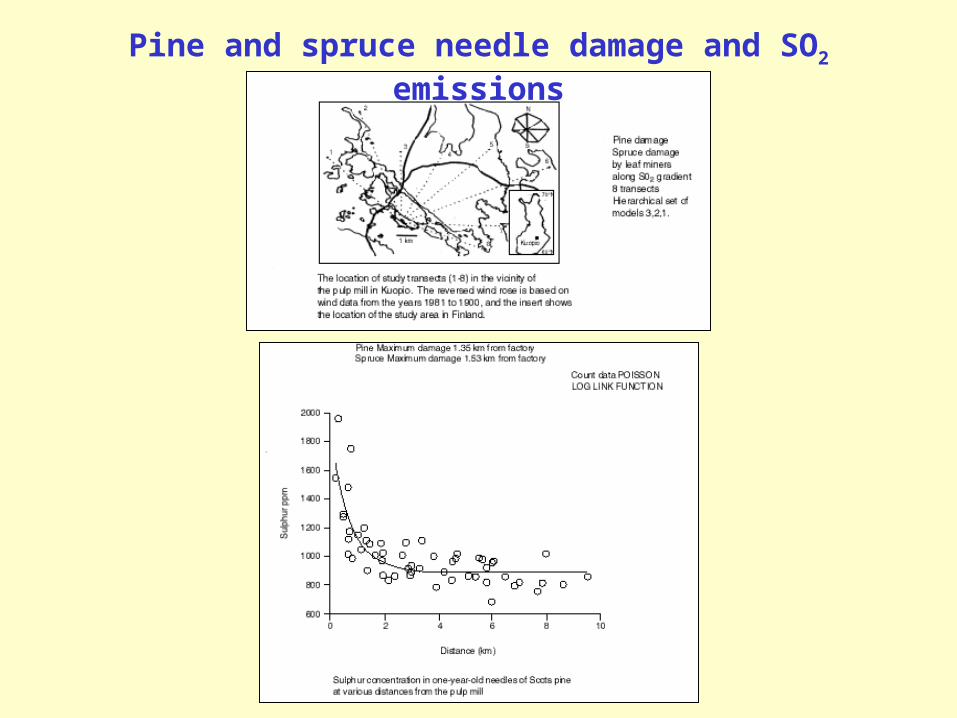
Pine and spruce needle damage and SO2 emissions


Predicted damages and their 95% confidence limits against sulphur concentration of Scots pine needles. The regression model was fitted with different levels (heights of the peaks) for the transects and using observed shoot lengths as offset; the lines shown correspond to transect 1 and 1cm shoot length

The Gaussian response curve for the abundance value (y) of a taxon against an environmental variable (x) (u = optimum or mode; t = tolerance; c = maximum).
Diatom – pH responses


yk(x) =
yk(x) is expected proportional abundance of taxon k
as a function of x (pH)
Generalised linear model
log = b0 + b1x + b2x2
where p is shorthand for yk(x)
2k
2k
2k
2k
t / )u-1/2(x-k
t / )u--1/2(xk
expc 1
expc
p1p
Gaussian Logit Model

Gaussian response function:GLM estimation
μ = h exp
log μ = b0 + b1x + b2x2
2
2
2tux )(
• Gaussian response function can be written as a generalized linear model (which is easy to fit)
- Linear predictor: explanatory variables x and x2
- Link function log (or logit)
- Error Poisson (or Binomial)
• The original Gaussian response parameters can be found by
u = -b1/2b2 OPTIMUM
t = TOLERANCE
h = exp(b0 - b12 / 4b2) HEIGHT
221 b


Results of fitting Gaussian logit, linear logit and null models to the SWAP 167-lake training set and lake-water pH
225 taxa
No. of taxa
Non-converging 1
Gaussian unimodal curves with maxima (b2 < 0)
88
Linear logit sigmoidal curves 78
Gaussian unimodal curves with minima (b2> 0)
5
No pattern 53
Significant Gaussian logit model 88
Significant linear logit model 78
Non-significant fit to pH 58

SEVERAL GRADIENTS
• Gaussian response can be fitted to several gradients: Bell-shaped models
J. Oksanen (2002)

INTERACTIONS IN GAUSSIAN RESPONSES
• No interactions: responses parallel to the gradients
• Interactions: the optimum on one gradient depends on the other
J. Oksanen (2002)
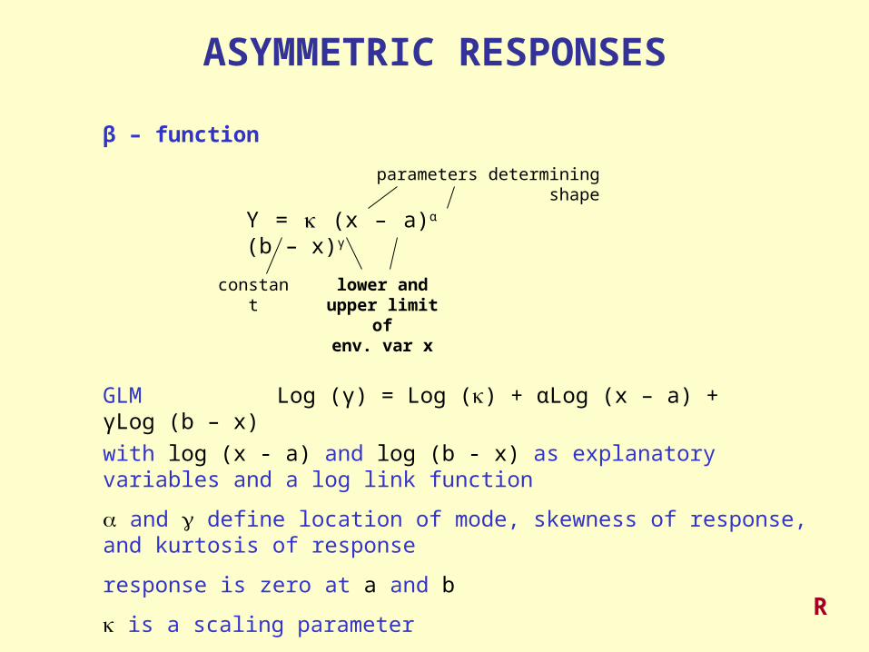
β – function
GLM Log (γ) = Log () + αLog (x – a) + γLog (b – x)
Y = (x – a)α (b – x)γ
lower and upper limit
ofenv. var x
constant
parameters determining shape
ASYMMETRIC RESPONSES
with log (x - a) and log (b - x) as explanatory variables and a log link function
and define location of mode, skewness of response, and kurtosis of response
response is zero at a and b
is a scaling parameterR

SELECTION OF RESPONSE MODELS

Huisman, Olff & Fresco (1993) – J. Veg. Sci. 4, 37–46
Huisman, Olff & Fresco - Hierarchical models of species-environment responses.
Environmental Environmental gradient gradient xx HOF
Plateau
III
Oksanen & Minchin (2002) - Ecol. Modelling 157, 119-129

HOF MODELS
J. Oksanen (2002)
Huisman-Olff-Fresco: A set of five hierarchic models with different shapes.
Model Parameters
V Skewed a b c d
IVSymmetric
a b c b
III Plateau a b c
IIMonotone
a b 0 0
I Flat a 0 0 0

M = sample total
(e.g. 100)
4 parameters to estimate
IV 3 parameters to estimate
II 2 parameters
I 1 parameter
Vy M
e ea bx c dx
1
1
1
1
y Me ea bx c bx
1
1
1
1
y Mea bx
1
1
y Mea
1
1
Hierarchical model means that a simpler model has (1) fewer parameters than the complex model and (2) can be derived by simplifying a more complex model by deleting one or more parameters.
y = expected value which is dependent on the known values of the environmental gradient x, maximum possible value (M), and parameters a, b, c, and d.
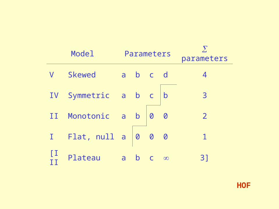
HOF
Model Parameters
parameters
V Skewed a b c d 4
IV Symmetric a b c b 3
II Monotonic a b 0 0 2
I Flat, null a 0 0 0 1
[III Plateau a b c 3]

HOF - fits most complex model V first by maximum likelihood, then IV, II and I (backward elimination)
- calculates deviance, if drop in deviance greater than 3.84, extra parameter is significant at p < 0.05 (2 distribution).
- if data are overdispersed (deviance > degrees of freedom), cannot use 2 test. Must use F-test.
- model is simplified as long as the removed parameters are not significant at p < 0.05
- can specify Poisson or binomial error function
pnD
DDF
p
pppn
/,1
1

HOF - estimation is stopped when first significant term is found
- evaluate how many taxa have significant fits to models V, IV, II and I
- adopt the simplest model which cannot be simplified without a significant change in deviance
- as model III (plateau) has the same number of parameters as model IV, not fitted routinely. If model IV is rejected in favour of model V, the latter is compared against model III and model simplification is continued
HOF

HOF: INFERENCES ON RESPONSE SHAPES
• Alternative models differ only in response shape
• Selection of most parsimonious model with statistical criteria
• 'Shape' is a parametric concept, and parametric HOF models may be the best way of analysing differences in response shapes. Most parsimonious HOF models
on altitude gradient in Mt. Field, Tasmania.
J. Oksanen (2002)

1. All models are wrong
2. Some models are better than others
3. The correct model can never be known with certainty
4. The simpler the model, the better it is In GLM may have mis-specified model, error
structure, or link function.
MODEL CRITICISMFaraway 2005, 2006

MODEL CRITICISM
Plot residuals against fitted values
For non-Normal models: Use Anscombe or Pearson residuals
Normality: Plot ordered residuals against a Normal deviate
Any pattern: Something wrong
Bent residual belt: Wrong systematic part
Wrong link function
Wrong or missing explanatory variables
Widening residual belt: Wrong error function
Leverage values show the influential observations
Influential observations: small residuals
Leverage > 2p/N is high

EXAMPLE OF MODEL CRITICISM

CLASSIFICATION
What has this to do with regression analysis?
What is classification as distinct from clustering and partitioning (Lecture 3) (= unsupervised pattern recognition)?
Classification involves multivariate data that fall into two or more a priori groups, so-called supervised pattern recognition
Range of questions that can be asked of such data.

1. Do the groups involved have different mean vectors for the available measurements?
Multivariate equivalent of familiar univariate t-test, Hotelling’s T2 and multivariate analysis of variance.
Linear discriminant analysis (2 groups) or multiple discriminant analysis (3 or more groups) (also known as canonical variates analysis).

2. For grouped multivariate data, it is possible to use the measurements to construct a classification rule derived from the original observations (training set) that will allow new individuals having the same set of measurements but no known group identity to be allocated to a group or classified in such a way that misclassifications are minimised.
A.H. Fielding (2007) Cluster and classification techniques for the biosciences. Cambridge University Press

Can formulate this classification problem as a regression problem
Response Variable Predictor Variable
Class 1 Class 2 x1, x2, x3, … xm
1 0 x1, x2, x3, … xm
1 0 x1, x2, x3, … xm
1 0 x1, x2, x3, … xm
0 1 x1, x2, x3, … xm
0 1 x1, x2, x3, … xm
0 1 x1, x2, x3, … xmRegression with 0/1 response variable(s) and predictor variables

DISCRIMINANT FUNCTION FOR SEXING FULMARINE PETRELS FROM EXTERNAL
MEASUREMENTS (Van Franketer & ter Braak (1993) The Auk, 110: 492-502)
Lack plumage characters by which sexes can be recognised.
Problems of geographic variation in size and shape.
Approach:
Five species of fulmarine petrels
Antarctic petrel Northern fulmar
Cape petrel Southern fulmar
Snow petrel
1. A generalised discriminant function from data from sexed birds of a number of different populations
2. Population – specific cut points without reference to sexed birds
HL – head length
CL – bill length
BD – bill depth
TL – tarsus length
Measurements

STEPWISE MULTIPLE REGRESSION
Ranks characters according to their discriminative power, provides estimates for constant and regression coefficient b1 (character weight) for each character.
For convenience, omit constant and divide the coefficient by the first-ranked character.
Discriminant score = m1 + w2m2 + ..... + wnmn
where mi = bi/b1
Cut point – mid-point between ♂ and ♀ mean scores.


Reliability tests
1. Self-test - how well are the two sexes discriminated? Ignores bias, over-optimistic
2. Cross-test - divide randomly into training set and test set
3. Jack-knife (or leave-one-out – LOO)
- use all but one bird, predict it, repeat for all birds. Use n-1 samples. Best reliability test.
Small data-sets - self-test OVERESTIMATE
- cross-test UNDERESTIMATE
- jack-knife RELIABLE

MULTISAMPLE DISCRIMINANT
ANALYSIS If samples of sexed birds in different populations are small but different populations have similar morphology (i.e. shape) useful to estimate GENERALISED DISCRIMINANT from combined samples.
1. Cut-point established with reference to sex(determined by dissection) WITH SEX
2. Cut-point without reference to sex NO SEXDecompose mixtures of distributions into their underlying components. Maximum likelihood solution based on assumption of two univariate normal distributions with unequal variances.
Expectation – maximisation (EM) algorithm to estimate means 1 and 2 and variances 1 and 2 of the normals.
Cut point is where the two normal densities intersect.
xs = (22 - 1
2)-1 {122 - 21
2 + 12 [(1 - 2)2
+ (12 - 2
2) log n 12/2
2]0.5}


Cleveland, W.S. 1979. J. Amer. Stat. Association 74, 829-836
Cleveland, W.S. 1993. Visualizing Data. AT & T Bell Laboratories
Cleveland, W.S. 1994. The Elements of Graphing Data. AT & T Bell Laboratories
Crawley, M.J. 2002. Statistical Computing – an introduction to data analysis using S-PLUS. Wiley
Efron, B. & Tibshirani, R. 1981. Science 253, 390-395
Trexler, J.C. & Travis, J. 1993. Ecology 74, 1629-1637
LOCALLY WEIGHTED REGRESSION

W. S. Cleveland LOWESS Locally weightedor regression scatterplotLOESS smoothing
May be unreasonable to expect a single functional relationship between Y and X throughout range of X.
(Running averages for time-series – smooth by average of yt-1, y, yt+1 or add
weights to yt-1, y, yt+1)
LOESS - more general
1. Decide how ‘smooth’ the fitted relationship should be.2. Each observation given a weight depending on distance to observation x1 for
adjacent points considered.3. Fit simple linear regression for adjacent points using weighted least squares.4. Repeat for all observations.5. Calculate residuals (difference between observed and fitted y).6. Estimate robustness weights based on residuals, so that well-fitted points
have high weight.7. Repeat LOESS procedure but with new weights based on robustness weights
and distance weights.
Repeat for different degree of smoothness, to find ‘optimal’ smoother.
LOCALLY WEIGHTED REGRESSION
R

(A)
Surv
ival ra
te (
an
gula
rly t
ransf
orm
ed
) of
tadpole
s in
a s
ing
le e
ncl
osu
re p
lott
ed a
s a f
un
ctio
n o
f th
e a
vera
ge b
ody m
ass
of
the s
urv
ivors
in t
he e
ncl
osu
re.
Data
fro
m T
ravis
(1
983).
Lin
e indic
ate
s th
e n
orm
al le
ast
-sq
uare
s re
gre
ssio
n. (B
) R
esi
duals
fro
m t
he lin
ear
regre
ssio
n d
epic
ted in P
art
A
plo
tted a
s a f
unct
ion
of
the in
dependent
vari
ab
le, avera
ge b
od
y m
ass
.
(A)
Data
fro
m a
bove w
ith a
lin
e d
ep
icti
ng a
least
-sq
uare
s quadra
tic
model. (
B)
Data
fro
m
above w
ith
a lin
e d
epic
ting
a L
OW
ESS
regre
ssio
n m
odel w
ith f
= 0
.67.
(C)
Data
fro
m a
bove
wit
h a
lin
e d
ep
icti
ng a
LO
WESS
regre
ssio
n m
odel w
ith f
= 0
.33.

How
the L
oess
sm
ooth
er
work
s. T
he s
had
ed r
eg
ion indic
ate
s th
e
win
dow
of
valu
es
aro
und t
he t
arg
et
valu
e (
arr
ow
). A
weig
hte
d lin
ear
regre
ssio
n (
bro
ken lin
e)
is c
om
pute
d,
usi
ng w
eig
hts
giv
en b
y t
he
“tri
cube”
funct
ion
(dott
ed lin
e).
Repeati
ng t
he p
roce
ss f
or
all
targ
et
valu
es
giv
es
the s
olid
curv
e.


An air pollutant, ozone, is graphed against wind speed. From the graph we can see that ozone tends to decrease as wind speed increases, but judging whether the pattern is linear or nonlinear is difficult.
Loess, a method for smoothing data, is used to compute a curve summarizing the dependence of ozone on wind speed. With the curve superposed, we can now see that the dependence of ozone on wind speed is nonlinear.

The three loess curves have three different values of the smoothing parameter, α. From the bottom panel to the top the values are 0.1, 0.3 and 0.6. The value of λ is 2.
α = “bandwidth” parameter
0.3-0.5
λ = polynomial order of fitted local regression model
Three loess fits are shown. From the bottom panel to the top, the two parameters, α and λ, are the following:
0.1 and 1; 0.3 and 1 and 0.3 and 2.

LOESS – STATISTICAL ASPECTS
Can express its complexity by the number of degrees of freedom (DF) taken from the data by the fitted model = equivalent number of parameters.
As LOESS produces fitted values of the response variable, can calculate variability in the response values accounted for by the LOESS fitted model and compare it with the residual sum of squares.
As we have the DF of the fitted model, can calculate residual DF and calculate sum of squares per one degree of freedom (corresponding to the mean square in an ANOVA table for a classical regression model).
Thus we can compare different LOESS models using an ANOVA approach of regression and residual sum of squares or deviance. Can also use generalised cross-validation to find ‘optimal’ LOESS model.
REF
REF
REF
REF

‘In any specific application of LOESS, the choice of the two parameters and must be based on a combination of judgement and trial and error. There is no substitute for the latter’
Cleveland (1993)

SPLINE FUNCTIONS
Given data of x and y variables on the same n objects, can connect these points with a smooth, continuous line – spline function.
Named from the flexible drafting spline made from a narrow piece of wood or plastic that can be bent to conform to an irregular shape.
Splines are not analytical functions and they are not statistical models like regressions.
Purely arbitrary and have no real theoretical basis except the theory that defines the characteristics of the lines themselves.
Extremely useful for interpolation for smoothing in two or three dimensions.
Faraway 2006, Crawley 2002

Splines are piecewise polynomials that are constrained to have continuous derivatives at the joints or knots between the pieces or segments.
Cubic spline consists of cubic polynomials which are functions of the form:
The curve defined by a cubic polynomial can pass exactly through four points. For a set of observations with n > 4, need to use a succession of polynomial segments.
To ensure that there are no abrupt changes in slope or curvature between successive segments, the polynomial function is not fitted to four points but only to two. This allows using additional constraints to ensure that the resulting spline has continuous first derivatives between segments (the slope of the line will be the same on either side of a joint) and continuous second derivatives (the rate of change in the slope of the line will not change across a joint).
A spline of degree n will have continuous derivatives across the points up to order n – 1.
34
2321 xxxy
R

Mathematical Explanation
A smoothly joined piecewise polynomial of degree n.
t1, t2, …, tn are a set of n values in the interval a, b so that a < t1 t2 … tn b.
Cubic spline is a function g such that on each of the intervals (a, t1), (t1, t2), …, (tn, b) is a cubic polynomial
and
the polynomial pieces fit together at the points t1 in such a way that g itself and its first and second derivatives are continuous at each ti and hence on the whole a, b.
The points ti are called knots.
REF
REF
REF
REF
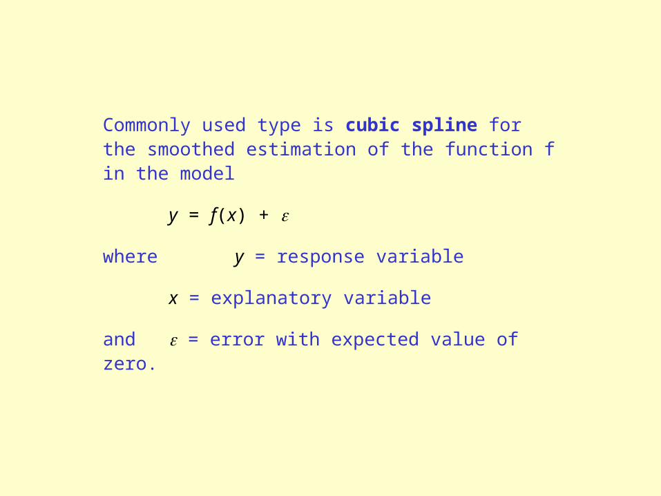
Commonly used type is cubic spline for the smoothed estimation of the function f in the model
y = f(x) +
where y = response variable
x = explanatory variable
and = error with expected value of zero.

Simple Use of Splines
Basic scatter plot of yield against irrigation
LOWESS fitted

Curve-fitting is trade off between smoothness and roughness. Concept of degrees of freedom serves as penalty.
Want smoothest graph that describes relationship between y and x that has the lowest penalty in terms of degrees of freedom.
2 degrees of freedom (slope and intercept)
linear fit
n degrees of freedom

3 df no hump 4 df hint of hump
6 df clear hump

Which to use?
Parsimony favours an asymptote (3 df) over a hump (4 or 6 df).
Need more data to test between asymptote and hump.
Splines are arbitrary smoothers.
S-PLUS
R

How is a spline fitted? Involves differential calculus.
Construct required estimator for the following minimisation problem, namely find f to minimise
where primes represent differentiation.
The first term is residual sum of squares which is used as a distance function between data and estimator.
The second term penalises roughness of the function.
Parameter 0 is a smoothing parameter (degrees of freedom) that controls trade-off between smoothness of the curve and the bias of the estimator.
Solution to the minimisation problem is a cubic polynomial between successive x-values with continuous first and second derivatives at the observation points.
uufxfyn
iii d)()(
211
1
2
REF
REF
REF

Uses of Splines
1. Interpolation for smoothing
2. Regression analysis including generalised additive models (GAM)
Ecological examplevan Dobben & ter Braak 1999 Lichenologist 31: 27-39

Lichens and Air Pollution in the Netherlands
1216 groups of 6 tree species in eight 750 km2 areas.104 lichen species, 65 in 10 or more tree groups.
Pollution data SO2, NO2, and NH3
high correlation between SO2 and NO2 (r =
0.49)
Four models fitted for each of the 65 lichen species
1) Abundance =
where coast = distance to coastdiameter = tree diametercj = regression coefficient for dummy (1/0)
variable for tree species j
j
j jcbbbbbb ) species tree(coastdiameterNHNOSO 54322210 3

2) Non-zero abundance =
j
j jcbbbbbb ) species tree(coastdiameterNHNOSO 54322210 3
3) Logit (1/0)
jj jcb
bbbbbp
p
) species tree(coast
diameterNHNOSO)1(
log
5
4322210 3
4) Logit with splines
jj jcb
bbbbbp
p
) species tree(coast
diameterNHNO)(SOSPL)1(
log
5
43222q10 3
where SPLq = spline function with q degrees of freedom (q = 1, 2, or 4)
In this context q = 2 allows fitting of a unimodal response, q = 4 bimodal response.
Find q by increasing q stepwise and stop if the resulting increase in fit is not significant at 1% level based on deviance test.

van Dobben & ter Braak, 1999

van Dobben & ter Braak, 1999
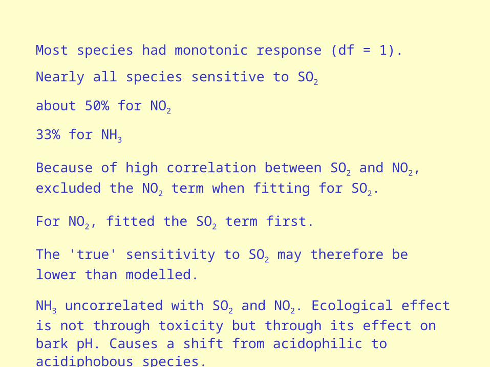
Most species had monotonic response (df = 1).
Nearly all species sensitive to SO2
about 50% for NO2
33% for NH3
Because of high correlation between SO2 and NO2, excluded
the NO2 term when fitting for SO2.
For NO2, fitted the SO2 term first.
The 'true' sensitivity to SO2 may therefore be lower than
modelled.
NH3 uncorrelated with SO2 and NO2. Ecological effect is not
through toxicity but through its effect on bark pH. Causes a shift from acidophilic to acidiphobous species.

Semi-parametric extension of generalised linear models GLM:GLM
intercept or constant predictor
variables
link function
p
jjj xxEyg
1
modelled abundance of response variable y
regression coefficients or model parameters
Requires a priori statistical model, e.g. Gaussian logit model, β-response model, etc.
What if the response is bimodal, is badly skewed, or is more complex than a priori model?
GLM may not be flexible enough to approximate the true response adequately. GLM are model-driven.
e.g. Ordinary least-squares regression - identity link, normal error distribution
Ey = + jxje.g. 2-dimensional Gaussian logit regression - logit link, binomial error distribution
22423
212111
xxxxp
pp
Log)( Logit
GENERALISED ADDITIVE MODELS (GAM)

GAM
modelled abundance of
response variable y
p
jjj xffxEyg
1
link function
unspecified smoothing functions estimated from data using
smoothers to give maximum explanatory power
intercept or constant predictor variables
fj are unspecified smoothing functions estimated from the data using
techniques developed for smoothing scatter plots, e.g. loess, cubic splines.
Data determine shape of response curve rather than being limited by the shapes available in parametric GLM. Can detect bimodality and extreme skewness.
Regression surface g(Ey) for taxon y is expressed as a sum of the functions for each variable xj so each has an additive effect, hence GAM.
GAM are data-driven, the resulting fitted values do not come from an a priori model. Still some statistical framework with link functions and error specification
Need to specify the type of smoother and their complexity in terms of their degrees of freedom.
R

GENERALISED ADDITIVE MODELS
Efron, B. & Tibshirani, R. 1991 Science 253, 390-395
Yee, T.W. & Mitchell, N.D. 1991 J. Vegetation Science 2, 587-602
Guisan, A. et al. 2002 Ecological Modelling 157, 89-100
Hastie, T.J. & Tibshirani, R. 1990 Generalized Additive Models. Chapman & Hall
Wood, S.N. 2006. Generalized Additive Models. An introduction with R. Chapman & Hall/CRC.

GENERALIZED ADDITIVE MODELS (GAM)
• Generalized from GLM; linear predictor replaced with smooth predictor
• Smoothing by regression splines or other smoothers
• Degree of smoothing controlled by degrees of freedom; analogous to number of parameters in GLM
• Everything else like GLM
• Enormous potential use in ecology J. Oksanen (2002)

“No more causes or factors should be assumed than are necessary to account for the facts”.
i.e. the simplest model desirable but with maximum explanatory power. Compromise between simple and complex models.
In GLM, we evaluate role of individual predictors by looking at the magnitude, sign and likely statistical contribution of the estimated regression coefficients. Fit most complex model first, and then backward eliminate variables until retain simplest but with good explanatory power.
In GAM, we can look at fitted smoothers to investigate how the influence of a particular predictor varies along the range of its possible values. Smoothers can be chosen to have different levels of detail that are characterised by the effective number of degrees of freedom used in the fitting of the smoother.
This concept, shared with regression analysis where the individual model terms correspond to one degree of freedom, allows in conjunction with the concept of residual deviance explained, to evaluate significance of the variability explained by the fitted additive models and to make decisions about the significance of any model improvements by extending from constant linear GLM GAM S(2) GAM S(3) GAM S(4).
Simple leave-one-out (jack-knife) to estimate realistic root mean square error of prediction (RMSEP).
PRINCIPLE OF PARSIMONY IN STATISTICAL MODELLING

DEGREES OF FREEDOM
J. Oksanen (2002)
The width of a smoothing window (span) = Degrees of Freedom

SWISS MODERN POLLEN AND CLIMATE


MULTIPLE GRADIENTS
J. Oksanen (2002)
• Each gradient is fitted separately
• Interpretation easy: Only the individual main effects shown and analysed
• Possible to select good parametric shapes
• Thin-plate splines: Same smoothness in all directions and no attempt at making responses parallel to axes


Two explanatory variables show interaction of effects if the effect of one variable depends on the value of the other.
Test for interaction by extending our regression equation with product terms, i.e.
GLM
GAM
Then test using F-test on deviance if contribution of interaction is significant.
Three groups of taxa based on most appropriate pairs of predictors.
p
jkjqjj xxxEyg
1
p
jkjqjj xxfxfEyg
1
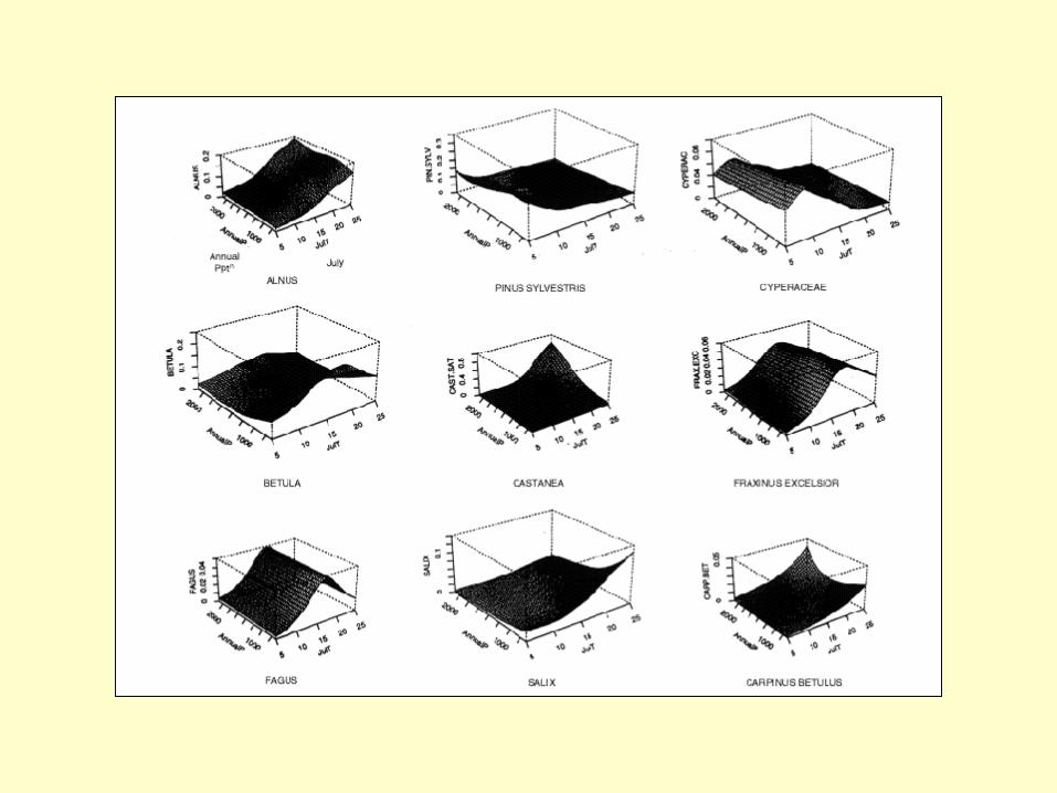
(1) (2) July temperature - Annual pptn
Pinus cembra Alnus, Pinus sylv
Selaginella selaginoides Fagus, Carpinus bet
Botrychium Betula, Salix
Gramineae (p =0.05) Fraxinus excelsior
Artemisia
Populus (3)
Platanus Non-significant interaction Quercus, Alnus viridis
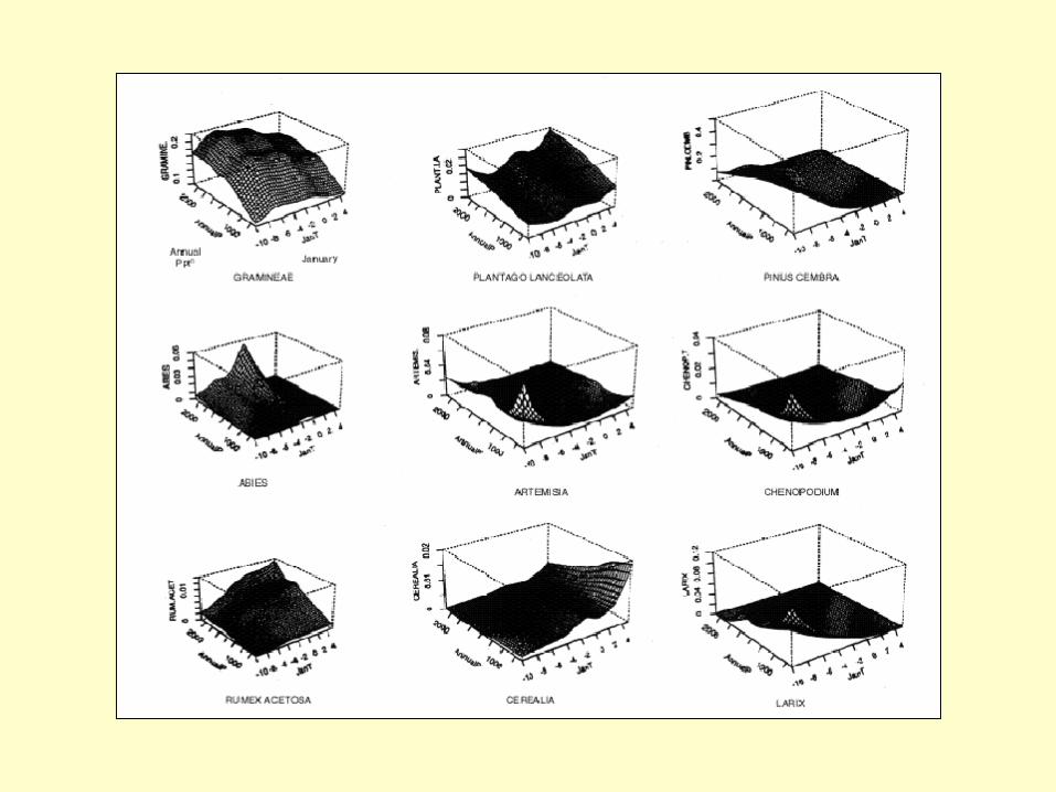
January temperature - Annual pptn
Significant interaction (p≤ 0.05)
Non-significant interaction
January temperature - July temperature
Significant interaction
Non-significant interaction
INTERACTIONS BETWEEN PREDICTORS ON RESPONSE OF TAXON

INTERACTIONS
GAM are designed to show clearly the main effects in GAM plots 'Equivalent kernel' is parallel to the axes
J. Oksanen (2002)
" "

Variables Model P(.) RAltitude s( ,3) <0.001 0.7Slope s( ,2) <0.001 0.21Aspect n.s.Rock pH poly( ,2) <0.001 0.82Rock Ca s( ,2) <0.001 0.81Water pH poly( ,2) <0.001 0.42Soil pH n.a.Soil Ca n.a.LOI n.a.Ri poly( ,3) <0.001 0.8Substratum Linear <0.001Flushing Quad <0.001Cracks Linear <0.001Weathering Linear <0.001Shelter Quad <0.001Undulation Linear <0.001Concavity Linear <0.001Snow-persistence Quad <0.001Phyllitite Linear <0.001Flush + Shelter Quad + Quad <0.001Flush + Snow Quad + Quad <0.001Shelter + Snow Quad + Quad <0.001Ri + Flush poly( ,1) + Quad <0.001 0.79
Ri + Shelter poly( ,1) + Quad <0.001 0.69
Ri + Snow poly( ,1) + Quad <0.001 0.61
Rock pH + Rock Ca s( ,3) + s( ,3) <0.001 0.67Rock pH + Water pH s( ,2) + s( ,3) <0.001 0.38Rock Ca + Water pH s( ,3) + s( ,3) <0.001 0.47
Interactions
Summary of regression statistics for Andreaea nivalis. Included are model typeselected, p-value, and regression coefficient (R) for continuous variables.Continuous variables; s( ,λ) = smooth spline function (GAM) where λ sets thewidth of the neineighbourhood, poly ( ,n) = GLM of the n’th order polynomial.Categorical variables; Linear = reflects a linear continuous function, Quad =reflects a quadratic continuous function. Not significant = n.s., not available = n.a.
ANDREAEA NIVALIS

The response function for A. nivalis on the continuous environmental variables: (a) altitude, (b) slope, (c) rock pH, (d) rock Ca, (e) water pH and (f) radiation index. = number of occurrences at each level of the gradient.
Histogram of A. nivalis on each categorical variable: (a) substratum, (b) flushing, (c) cracks, (d) weathering, (e) shelter, (f) undulation, (g) concavity, (h) snow-persistence, and (i) phyllite.

Response surface of A. nivalis on: (a) shelter and flushing, (b) flushing and radiation, (c) snow-persistence + flushing, and (d) snow-persistence + shelter.

Response surface of A. nivalis on: (a) rock Ca and rock pH, (b) water pH and rock pH, and (c) water pH + rock Ca.

GENERALISED ADDITIVE MODELS – A SUMMARY
GAMs are semi-parametric extensions of GLMs.
Only underlying assumptions are that the functions are additive and that the components are smooth. Like GLM, uses a link function to establish a relationship between the mean of the response variable and a 'smoothed' function of the predictor variable(s).
Strength is ability to deal with highly non-linear and non-monotonic relationships between the response variable and the set of predictor variables.
Data-driven rather than model-driven (as in GLM). Data determine the nature of the relationship between response and predictor variables.
Can handle non-linear data structures. Very useful exploratory tool.

A CONTINUUM OF REGRESSION MODELS
Simple Linear Regression Multiple Linear Regression > GLM > GAM
SLR and MLR - most restrictive in terms of assumptions but are most used (and misused!)
GLM - fairly general but still model-based
GAM - most general as data-based

Breiman, L., Friedman, J., Ohlson, R. & Stone, C. 1984. Classification and regression trees – Wadsworth
De'Ath, G. 2002 Ecology 83, 1105-1117
De'Ath, G. & Fabricus, K.E. 2000 Ecology 81, 3178-3192
Efron, B. & Tibshirani, R. 1991. Science 253, 390-395
Michaelsen, J. et al. 1994. J. Vegetation Science 5, 673-686
CLASSIFICATION AND REGRESSION TREES (CART)
Also known as decision trees

Decision Trees
Like a species identification key. Class labels are assigned to objects by following a path through a series of simple rules or questions, the answers to which determine the next direction through the path.
Decision tree is a supervised learning algorithm which must be provided with a training set that contains objects with class labels.
Looks like a cluster analysis dendrogram or partitioning diagram but these are from unsupervised methods that take no account of pre-assigned class labels.

Example (three species of Iris)
If petal length < 2.09 cm Iris setosaIf petal width < 1.64 cm Iris versicolorIf neither Iris virginica
Fielding 2007As axis-parallel splits

CART PROBLEM:
Experiment on cause of duodenal ulcers, one of 56 model nucleophiles were given to each of 745 rats. Each rat subsequently autopsied to check for development of duodenal ulcer and outcome scored as 1, 2 or 3 severity.
535 class 1, 90 class 2, 120 class 3 outcomes
Which of 67 characteristics of these compounds was associated with development of duodenal ulcers?
CART aims to use a set of predictor variables to estimate the means of one or more response variables. A binary tree is constructed by repeatedly splitting the data set into subsets. Each individual split is based on a single predictor variable and is chosen to minimise the variability of the response variables in each of the resulting subsets.
The tree begins with the full data set and ends with a series of terminal nodes. Within each terminal node, the means of the response variables are taken as predictors for future observations.
Closer to ANOVA than regression in that data are divided into a discrete number of subsets based on categorical predictors and predictions are determined by subset means.
R

Measure of impurity
Univariate response variable error sum of squares, i.e. one-way ANOVA at each split and selecting the predictor variable which minimises the error sum of squares in the two descendent nodes.
Categorical responses (classes 1, 2, 3) – assign classes to terminal node using majority rule, assign the class that is most numerous in the node.
At each node of the tree a question is asked – data points for which the answer is yes are assigned to the left branch.
May be less desirable to misclassify animal with a severe ulcer. Introduce a higher penalty to errors for class 3.
Must define two criteria:
1. A measure of impurity or inhomogeneity.
2. Rule for selecting optimum tree.
Produce a very large tree and then prune it into successively smaller trees. Skill of each tree is determined by cross-validation. Divide the full data into subsets, drop one subset, grow the tree on the remaining data and test it on the omitted subset.

CART tree. Classification tree from the CART analysis of data on duodenal ulcers. At each node of the tree, a question is asked; data points for which the answer is “yes” are assigned to the left branch and other data points are assigned to the right branch
Misclassification 1 39.6%
class 2 56.7%
3 18.3%R

CLASSIFICATION AND REGRESSION TREES – A
SUMMARYExplain variation of single response variable by one or more explanatory or predictor variables.
Response variable can be quantitative (regression trees) or categorical (classification trees).
Predictor variables can be categorical and/or quantitative.
Trees constructed by repeated splitting of data, defined by a simple rule based on single predictor variable.
At each split, data partitioned into two mutually exclusive groups, each of which is as homogeneous as possible. Splitting procedure is then applied to each group separately.
Aim is to partition the response into homogeneous groups but to keep the tree as small and as simple as possible.
Usually create an overlarge tree first, pruned back to desired size by cross-validation.
Each group typically characterised by either the distribution (categorical response) or mean value (quantitative response) of the response variable, group size, and the predictor variables that define it.

SPLITTING PROCEDURES
Way that predictor variables are used to form splits depends on their type.
1. Categorical variable with two levels (e.g. small, large), only one split is possible, with each level defining a group.
2. Categorical variables with more than two levels, any combination of levels can be used to form a split. With k levels, there are 2k-1 –1 possible splits.
3. Quantitative predictor variables, a split is defined by values less than and greater than some chosen value. Only the rank order of quantitative variables determines a split, and for u unique values there are u-1 possible splits.
From all possible splits of predictor variables, select the one that maximises the homogeneity of the two resulting groups. Homogeneity can be defined in many ways, depending on the type of response variable.
Trees drawn graphically, with root node representing the undivided data at the top, and the branches and leaves (each leaf representing a final group) beneath. Can also show summary statistics of nodes and distributional plots.
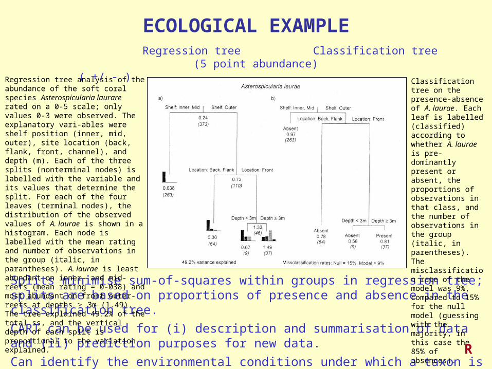
ECOLOGICAL EXAMPLE Regression tree Classification tree (5 point abundance) ( +/ - )
Splits minimise sum-of-squares within groups in regression tree; splits are based on proportions of presence and absence in the classification tree.
CART can be used for (i) description and summarisation of data and (ii) prediction purposes for new data.
Can identify the environmental conditions under which a taxon is particularly abundant (regression tree) or particularly frequent (classification tree).
Regression tree analysis of the abundance of the soft coral species Asterospicularia laurare rated on a 0-5 scale; only values 0-3 were observed. The explanatory vari-ables were shelf position (inner, mid, outer), site location (back, flank, front, channel), and depth (m). Each of the three splits (nonterminal nodes) is labelled with the variable and its values that determine the split. For each of the four leaves (terminal nodes), the distribution of the observed values of A. laurae is shown in a histogram. Each node is labelled with the mean rating and number of observations in the group (italic, in parantheses). A. laurae is least abundant on inner- and mid-reefs (mean rating = 0-038) and most abundant on front outer-reefs at depths 3m (1.49). The tree explained 49.2% of the total ss, and the vertical depth of each split is proportional to the variation explained.
Classification tree on the presence-absence of A. laurae. Each leaf is labelled (classified) according to whether A. laurae is pre-dominantly present or absent, the proportions of observations in that class, and the number of observations in the group (italic, in parentheses). The misclassification rate of the model was 9%, compared to 15% for the null model (guessing with the majority, in this case the 85% of absences).
R

Regression trees explaining the abundances of the soft coral taxa Efflatounaria, Sinularia spp., and Sinularia flexibilis in terms of the four spatial variables (shelf position, location, reef type, and depth) and four physical variables (sediment, visibility, waves, and slope). At the bottom of the cross-validation plots (a, d, g), the bar charts show the relative proportions of trees of each size selected under the 1-SE rule (grey) and minimum rules (white) from a series of 50 cross-validations. For Efflatournaria (a), a five-leaf tree is most likely by either the 1-SE or the minimum rule. For Sinularia spp. (d), five- to eight-leaf trees have support, and for S. flexibilis (g), five- to nine-leaf trees have support. Cross-validation plots (a, d, g), representative of the modal choice for each taxa according to the 1-SE rule, are also shown. For all three taxa, a five-leaf tree was selected (c, f, i). The shaded ellipses enclose nodes pruned from the full trees (b, e, h), each of which accounted for > 99% of the total ss.


COMPARISON OF CART AND GLMs
ANOVA is powerful technique but as number of predictor variables and complexity of data increase (interactions, unbalanced designs, empty cells), ANOVA and GLMs become less effective.
CARTs are simpler and less sensitive to unbalanced designs and zero-values. Splits represent an optimum set of one-degree-of-freedom contrasts.
Simple, easy to interpret, and graphical.
These CART advantages increase as number of predictor variables and complexity increase.
'Data mining' tool.

MULTIVARIATE REGRESSION TREES
De'Ath, G. 2002 Ecology 83, 1105-1117
Natural extension of univariate regression trees. Considers multivariate response, not single response.
Replace univariate response by multivariate assemblage response and redefine the impurity of a node by summing the univariate impurity measure over the multivariate response.
Extend univariate sum-of-squares impurity criterion to multivariate sum-of-squares about the multivariate mean. Sum of squared Euclidean distances (SSD) of samples about the node centroid.
Each split minimises the SSD of samples from the centroids of the nodes to which they belong. Maximises the SSD between node centroids (cf. k-means clustering). This minimises SSD between all pairs of samples within nodes and maximises SSD between all pairs of samples in different nodes.
Each tree leaf can be characterised by multivariate mean of its samples, number of samples at the leaf, and the predictor values that define it.
Forms clusters of sites by repeated splitting of data, each split defined by simple rule based on environmental values. Splits chosen to minimise the dissimilarity of sites within node.
R

MULTIVARIATE REGRESSION TREES (cont)
MRT is a form of constrained clustering, with constraints set by the predictor variables and their values
MRT can be extended to dissimilarity measures other than squared Euclidean distance (distance-based MRT)
Hunting spider data (12 species, 28 samples, six environmental variables)
Four-leaf tree split just on water content and abundances of fallen twigs at sample sites explains 78.8% of the species variance
Tree size selected by cross-validation. Four-leaf tree has lowest estimated prediction error
Can identify indicator species using Dufrêne & Legendre (1967) INDVAL approach


Tabulate explained variance at each split for each species
MULTIVARIATE REGRESSION TREES (cont)
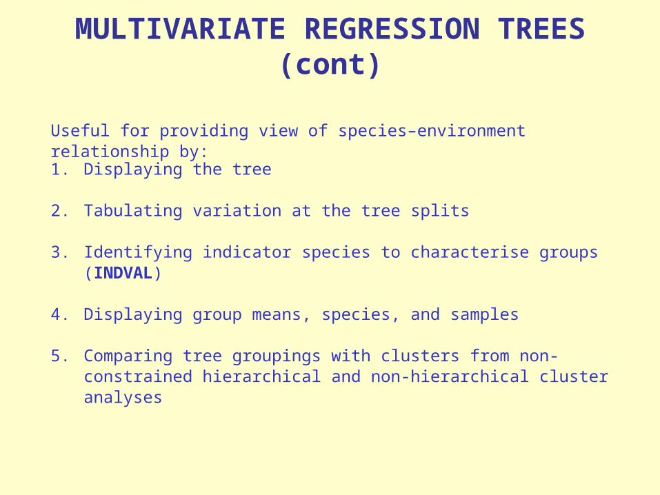
Useful for providing view of species–environment relationship by:
1. Displaying the tree
2. Tabulating variation at the tree splits
3. Identifying indicator species to characterise groups (INDVAL)
4. Displaying group means, species, and samples
5. Comparing tree groupings with clusters from non-constrained hierarchical and non-hierarchical cluster analyses

MULTIVARIATE REGRESSION TREES (cont)
Advantages
1. Absence of model assumptions (e.g. response models), resulting in greater robustness
2. Invariance to monotonic transformations of predictor variables
3. Prediction of species abundances from environmental variables
4. Emphasises local structure and interactions whereas constrained ordinations consider global structure
5. Outperforms or matches redundancy analysis and canonical correspondence analysis in explaining and predicting species composition
6. MRT is one tree, need m univariate regression trees for m species
7. More regression-based approach than simple discriminants and TWINSPAN

OTHER NEWER TYPES OF CLASSIFICATION AND REGRESSION
TREE TECHNIQUES
Rapidly growing area of activity in data-mining – analysis of large heterogeneous data
New approaches
1. Bagging Trees
2. Random Forests
3. Multivariate adaptive regression splines (MARS)
Brief introduction to each, so that you are aware of their existence and what their strengths and limitations are.

BAGGING TREES
Part of the output error in a simple regression tree (RT) can be due to the specific choice of the data set.
If create data sets by resampling with replacement (i.e. bootstrapping) and grow regression trees without pruning or averaging, the variance of the output error is reduced.
In bootstrapping. on average 37% of the data is excluded. The included data are replicated so that the sample is full size.
Portion of data in sample is ‘in-bag’ data, the rest is ‘out-of-bag’ data.
Out-of-bag data used not to build or prune tree but to provide better estimates of node error.
Requires 30-100 trees. Difficult or impossible to examine them all. Usually find consistent results, so one RT is adequate. Often averaged.
R

In addition to bagging, there is boosting or boosted trees (De’ath 2007 Ecology 88: 243-251)
In boosted trees, bias is reduced by repeatedly re-adjusting weights of the training samples. Used primarily for classifying data with large sample sizes rather than for regression.
R

RANDOM FORESTS (RF)
Designed to produce accurate predictions that do not overfit the data. Similar to BT in that bootstrap samples are drawn to construct multiple trees.
Difference from BT is that each tree is grown with a randomised set of predictors, hence name ‘random’ forests.
Large number of trees (500-2000) are grown, hence a ‘forest’ of trees.
Number of predictors used to find the best split at each node is a randomly chosen subset of the total number of predictors.
As with BT, trees are grown to maximum size without pruning. Aggregation is by averaging trees.
Out-of-bag samples can be used to derive an unbiased error rate and variable importance, eliminating the need for an independent test-set.

As many trees are grown, there is limited generalisation error (true error as opposed to training error only). Thus no overfitting is possible, hence good for prediction.
By growing each tree to maximise size without pruning and selecting only the best split between a random sub-set at each node, RF tries to maintain some predictive ability while inducing diversity among trees.
Random prediction selection diminishes correlation between unpruned trees and keeps bias low. Using an ensemble of unpruned trees, variance is also reduced.

Another advantage is that predicted output depends only on one user-selected parameter, the number of predictors to be chosen at each node.
RF seem more of a ‘black box’ than BT because cannot see individual trees. RF give general metrics to aid interpretation, especially the importance of predictor variables in prediction. Can evaluate how much worse the prediction would be if that predictor were permuted randomly.
In contrast to artificial neural networks that are very much a very ‘black box’, RF are perhaps a ‘grey box’. R

MULTIVARIATE ADAPTIVE REGRESSION SPLINES (MARS)
Builds flexible regression models by using basic functions to fit separate splines to distinct intervals of the predictor variables.
The variables to use and the end-points of the intervals are found by an exhaustive search procedure using basic functions. Differs from classical splines where the knots are pre-determined and evenly spaced.
Basic functions are similar to principal components and express the relationship of the predictors to the response variable.
MARS finds the locations and number of required knots in a forward/backward stepwise fashion.

Model is overfitted by generating more knots than needed, and the knots that contribute least to the overall fit are removed.
MARS have advantage over RT in the RT’s discontinuous branching at tree nodes is replaced with continuous smooth functions that are guided by the nature of the data.

MARS better at detecting global and linear data structure as output is smoother and not as coarse-grained and discontinuous as in RT.
MARS limitations are:
1. basic functions may be excessively guided by the local nature of the data, resulting in inappropriate results
2. selecting the correct values for the parameters can be cumbersome and may need multiple trial-and-error steps
3. does not lend itself well to modelling species-environment relationships
R

Comparison of regression-tree approaches
1. Method
RT Recusively partitions data based on a single, best predictor to form a binary tree. Creates a series of decision rules based on the predictor variables.
BT Creates multiple boot-strapped regression trees without pruning and averages the outputs.
RF Similar to BT except that each tree is grown with a randomised subset of predictors. Typically 500-2000 trees are grown and results aggregated by averaging.
MARSBuilds localised regression models by fitting separate splines using basic functions to distinct intervals of predictor variables.

2. Strengths
RT Better than conventional linear techniques in allowing for interactions and non-linearities when there are many predictors. Easy to interpret and can map predictors with greatest influence.
BT Very effective in reducing variance and error in high-dimensional data. Data not used (out-of-bag data) used to provide reliable error estimates
RF Growing large numbers of trees does not overfit the data, and random predictor selection keeps bias low. Provides good (?best) models for prediction.
MARSBecause splitting rules are replaced by continuous smooth functions, MARS better at detecting global and linear data structures. Output is smoother and less coarse-grained.

3. Limitations
RT Linear function highly approximated and output tree can be highly variant to small data perturbations.
BT Because large numbers of trees (30-50) are averaged, interpretation of results not easy. Bias component of the error is marginally better than single RT
RF At least a ‘grey box’ or a pale black box compared to BT. Can be very demanding in computing resources and time.
MARSTends to be excessively guided by the local nature of the data, making predictions with new data unstable. Selecting values for input parameters can be cumbersome.

MAJOR FEATURES OF CLASSIFICATION AND REGRESSION TREES OF
ECOLOGICAL DATA
1. Ability to use different types of response variables (continuous, categorical, +/-)
2. Capacity for interactive exploration, description, and prediction
3. Invariance to monotonic transformations of predictor variables
4. Easy graphical interpretation of complex results involving interactions
5. Model selection by cross-validation
6. Good procedures for handling missing values in both the response and the predictor variables

Recursive partition of data on the basis of set of predictor variables (in discriminant analysis a priori groups or classes, 1/0 variables).
Find the best combination of one variable and its split threshold value that separates the entire sample into two groups that are internally homogeneous as possible with respect to species composition.
Lindbladh et al. 2002. American Journal of Botany 89: 1459-1476
Picea pollen in eastern North America.
Three species P. rubens
P. mariana
P. glauca
CLASSIFICATION (= DISCRIMINANT ANALYSIS) AND CLASSIFICATION AND
REGRESSION TREES
R

Lindbladh et al. (2002)
R

Lindbladh et al. (2002)

Cross-validation of classification tree
(419 grains in training set, 103 grains in test set)

Binary trees -
Picea glauca vs rest
Picea mariana vs rest
Picea rubens vs rest

In identification can have several outcomes
e.g. not identifiable at all
unequivocally P. rubens
P. rubens or P. mariana, etc.

Can now see which grains can be equivocally identified in test set, how many are unidentifiable, etc. Assessment of inability to be identified correctly.
Unidentifiable about the same for each species, worst in P. mariana.
Test set (%)
P. glauca
P. mariana
P. rubens
Correct (100, 010, 001) 79.3 70.0 75.9
Equivocal (101, 110, 011, 111)
0.0 2.7 2.5
Unidentifiable (000) 20.7 27.3 21.6

Applications to fossil data


Relationship of the frequency of Fagus sylvatica to altitude and annual precipitation
Leps & Smilauer (2000)
EXAMPLES OF MODERN REGRESSION ANALYSIS

LINEAR
SECOND ORDER POLYNOMIAL
LINEAR LEAST SQUARES REGRESSION
Negative prediction
s
Two linear models describing, separately, the dependency of Fagus frequency upon altitude and annual precipitation
Shape of two generalized linear models describing, separately, the dependency of Fagus frequency upon altitude and annual precipitation
GLM POISSON LOG LINK FUNCTION
SECOND ORDER POLYNOMIAL
SECOND ORDER POLY-
NOMIAL
Leps & Smilauer 2000
GLM
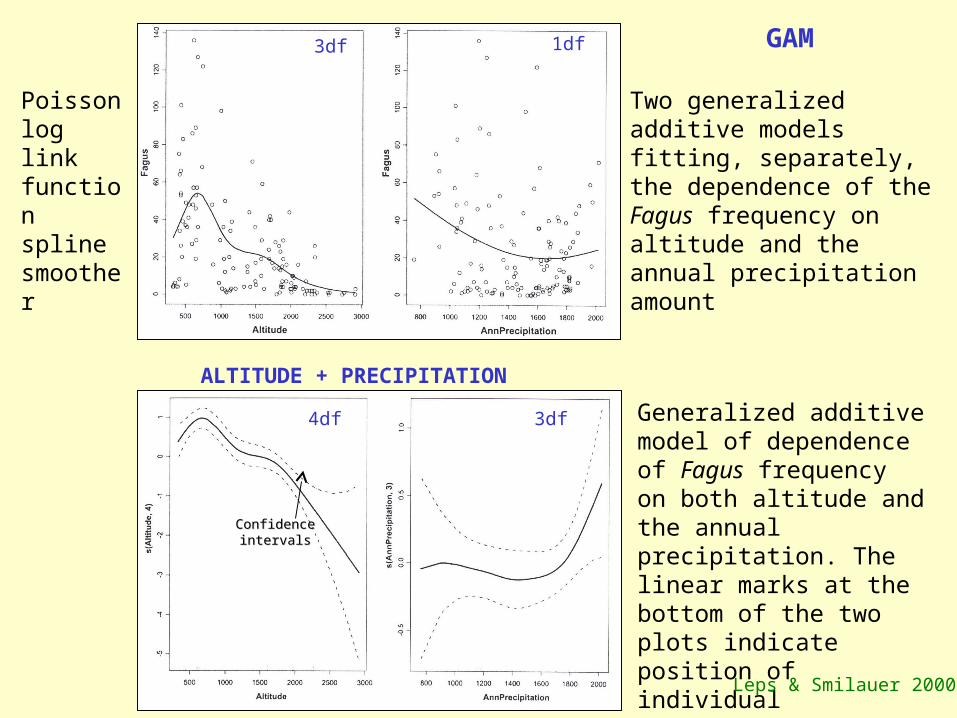
3df 1df
Poisson log link function spline smoother
GAM
Two generalized additive models fitting, separately, the dependence of the Fagus frequency on altitude and the annual precipitation amount
ALTITUDE + PRECIPITATION
Generalized additive model of dependence of Fagus frequency on both altitude and the annual precipitation. The linear marks at the bottom of the two plots indicate position of individual observations
4df 3df
Confidence Confidence intervalsintervals
Leps & Smilauer 2000

Comparison of three response surfaces modelling the frequency of Fagus using altitude and annual precipitation as predictors and using (from left to right) GLM, GAM, and loess smoother.
Leps & Smilauer 2000

Regression tree
Altitude, precipitation, degree days
The final regression tree
Fagus frequency
Leps & Smilauer 2000

Correlation between rate of sea-level change and frequency of explosive volcanism in the Mediterranean.V.J. McGuire, R.J. Howarth, C.R. Firth, A.R. Solow, A.D. Pullens, S.J. Saunders, I.S. Stuart, J.C Vita-Finzi (1997) Nature 389: 473-476
Location map of principal volcanic centres and provinces active in the Mediterranean region during the late Quaternary, and the distribution of boreholes from which deep-sea cores were extracted. The Roman Province includes the Vulsini, Vico, Sebatini and Albani centres; the Campanian Province includes Campi Flegrei, Somma Vesuvius and Ischia.
Cumulative plot of ordered event times (representing the tephra-layer occurrence) versus time. The dashed line corresponds to a median repose period of 1.05kyr. Three anomalous episodes of increased tephra-layer emplacement between 8 and 15, 34 and 38, and 55 and 61 kyr BP are also shown, having median repose periods (time to next tephra-producing event) of 0.35, 0.45 and 0.80 kyr respectively.

Changes in mean sea level. a. Estimated change in mean sea level (MSL) as a function of age (kyr) based on data from Barbados and Pacific cores. A smooth curve has been fitted to the Barbados data and region of overlap of the two data sets using the non-parametric locally weighted regression smoother LOWESS technique. The sparse data of Shackleton for the period 80 kyr ago have been fitted with a smooth cubic spline curve. Ages of dated tephra layers in deep-sea cores are shown by crosses. b. Rate of change of MSL with time, based on 0.25-kyr intervals. Ages of dated tephra layers in deep sea cores are shown by crosses.
Variation of repose times as a function of rate of change of mean sea level with time. These data are based on a bin width of 1.5d(MSL)/dt, and are summarized by box plots. Box width is proportional to the number of values in each bin; the base, horizontal dividing line, and top of each box show the 25th, 50th, (median) and 75th percentiles. In a few cases the median coincides with the base or top of the box; whiskers extend out to the most extreme values lying with 1.5 of the interquartile range beyond the ends of the box. Isolated data points are shown individually. The bold, solid curve is a weighted LOWESS- smoothed fit to the medians and indicates a clear decrease in repose period with rate of change of MSL, either upwards, (positive) or downwards (negative). We note that the maximum repose period is offset from the zero point on the rate of change axis, implying a time lag in the response of the volcanic systems to a given rate of change in the sea-level record. the dashed lines show the median line (line labelled ‘1’) and empirical 95% (‘2’) and 99% (‘3’) confidence envelopes for the binning and LOWESS curve-fitting process applied to 1,000 sets of 81 repose times drawn randomly from the empirical cumulative distribution of the observed repose times. No systematic variation of repose period with rate of change of MSL is apparent in the simulated data.
9595%%
9595%%

Branch of artificial intelligence - ability to “learn”.
Attempt to emulate the human brain with 1.5 x 10¹⁰ neurons each with 10 to 104 connections or synapses. Learn some target values or vectors from a set of associated input signals through a set of iterative adjustments of set of parameters. Minimise error between network and desired output following some learning rule. Mimic biological neuron. Regression, calibration, discriminant analysis (= classification)
ARTIFICIAL NEURAL NETWORKS

NEURAL NETWORKS – BASIC REFERENCES
Abdi, H. et al. 1999 Neural Networks. Sage Publications
Eberhart, R.C. & Dobbins, R.W. (eds.) 1990 Neural Network PC Tools. Academic Press
Faraway, J.J. 2006 Extending the Linear Model with R. Chapman & Hall/CRC (chapter 14)
Lek, S. & Guégan, J.P. 1999 Ecological Modelling 120, 65-73
Lek, S. & Guégan, J.P. 2000 Artificial Neuronal Networks. Application to Ecology and Evolution. Springer

(a) A diagram showing the general architecture of a three-layer back propagation network with five neurons in the input layer, three neurons in the hidden layer, and two neurons in the output layer. Each neuron in the hidden and output layers receives weighted signals from each neuron in the previous layer. (b) A diagram showing a single neuron in a back propagation network. In forward propagation, the incoming signals from the neurons of the previous layer (p) are multiplied with the weights of the connections (w) and summed. The bias (b) is then added, and the resulting sum is filtered through the transfer function to produce the activity (a) of the neuron. This is sent on to the next layer or, in the case of the last layer, represents the output. (c) A linear transfer function (left) and a sigmoidal transfer function (right)
All neurons are associated with:
Weight terms contain knowledge of memory of network.
Training involves incremental adjustment of weights to find an optimal mapping between input and output vectors. Need training set with corresponding inputs and outputs.
Optimisation ‘template comparison’ in which differences between actual output and desired output are used as optimisation criterion.
repeated until the differences between target output and computed output reach a preset threshold.
FORWARD PROPAGATION
Each input vector is propagated through network while being modified and filtered by the weights of the connections and by the transfer functions of the neurons. All incoming signals are multiplied with connective weights and summed and filtered through transfer function. Resulting activity of neuron is then used as input to next layer. Done once when running an already trained network.
TRANSFER FUNCTION Summed signals, filters and sends them on
BIAS TERM Measure of ‘importance’ like regression coefficients
Training -1 forward propagation
-2 back propagation

BACK PROPAGATION
Difference or ‘error’ between output vector resulting from forward propagation step and desired target vector is computed. Used to incrementally adjust the weights between output layer and the last of the hidden layers according to a learning algorithm based on a gradient-descent method.
For each layer, going backwards through the network, the values used for adjusting the weights are the error terms in the immediately succeeding layer. Size of incremental adjustments determined by learning rule set to 0–1.
Too high a learning rate may result in a network that may never converge. Too low a rate may result in excessively slow learning.
Various ways of doing back propagation:
Nguyen - Widrow initialisation
Momentum
Adaptive learning
Success of NN model best determined by some cross-validation.
Predictor or training set and independent test set leave-one-out (jack-knifing).
Statistics MSE RMSE r2 MSEP RMSEP
r2 cv
Estimated Predicted cross-validation

FOR AGR OTH PRE FLO ANI CTP COP ETP EOP(%) (%) (%) (cm) (m3s-1) (animal
km-2)(mg.l-1) (mg.l-1) (mg.l-1) (mg.l-1)
Minimum 0 0 0 13 0.001 0 0.005 0.005 0 0Maximum 100 100 100 263 14.65 233.5 1.12 0.58 321.7 117.7Range 100 100 100 250 14.65 233.5 1.12 0.57 321.7 117.7Mean 47.11 35.37 17.52 105.86 0.51 22.28 0.07 0.03 17.81 7.65Median 48.3 26.9 7.7 102 0.25 16.1 0.04 0.01 11.7 4.7Standard
deviation 32.35 32.61 22.84 41.57 0.99 25.06 0.09 0.05 22.33 10.62CV (%) 68.67 92.2 130.35 39.27 195.35 112.46 126.05 157.28 125.38 138.77Q1 16.1 3.6 2.7 81 0.09 1.4 0.02 0.008 6.4 2.8Q3 76.2 62.5 23.1 27 0.55 34.1 0.09 0.03 22.3 8.7
Statistical parameters of the variables studied(Q1, Q3: first and third quartile; CV: coefficient of variation)
PREDICTORS RESPONSES
Description of the data usedThe data used in this study come from the US National Eutrophication Survey (NES) as published by Omernik (1977). They consist of 927 tributary sites that drained watersheds not affected by point-source pollution. For each tributary site, the NES collected parameters for each subdrainage area: area, land use percentage (7 categories), geology, slope, pH, precipitation, flow and animal density. Moreover, mean nutrient concentrations of total phos-phorus, ortho-phosphate and nitrogen were measured in the corresponding tributaries and the export coefficients were calculated. These data were discussed by Omernik (op. Cit.). In the present study, we consider as indepen-dent variables: the percentage of the subwatershed areas under forest (FOR), agriculture (AGR), other categories (OTH) (defined as the difference between total watershed area and forest plus agriculture area), animal density (ANI), average annual precipitation (PRE) and flow (FLO). Concentration of total phosphorus (CTP), concentration of ortho-phosphorus (COP), export of total phosphorus (ETP) and export of ortho-phosphorus (EOP) were used as dependent variables. Independent variables presented large ranges corresponding to the large geographical variations in climate, soil characteristics and land use within the US territory (see table below). Dependent variables also presented large ranges with extremely high values. We can only hypothesize the existence of some local particularities, or the hidden effects of point source pollution not considered in the original data.

Representation of the structure of the neural network used. F1: input layer neurons, F2: hidden layer neurons, F3: output layer neurons. FOR: % forest; AGR: % agricultural zone; OTH: % other than forest and agriculture; PRE: precipitation; FLO: flow; ANI: animal density; Ŷ: estimated dependent variable.
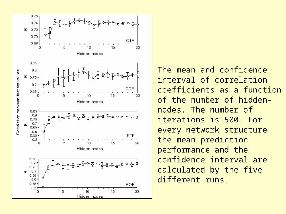
The mean and confidence interval of correlation coefficients as a function of the number of hidden-nodes. The number of iterations is 500. For every network structure the mean prediction performance and the confidence interval are calculated by the five different runs.

Mean Square of Errors (MSE) as a function of the number of training iterations. The number of hidden units is 5.
Lek et al. (1996)
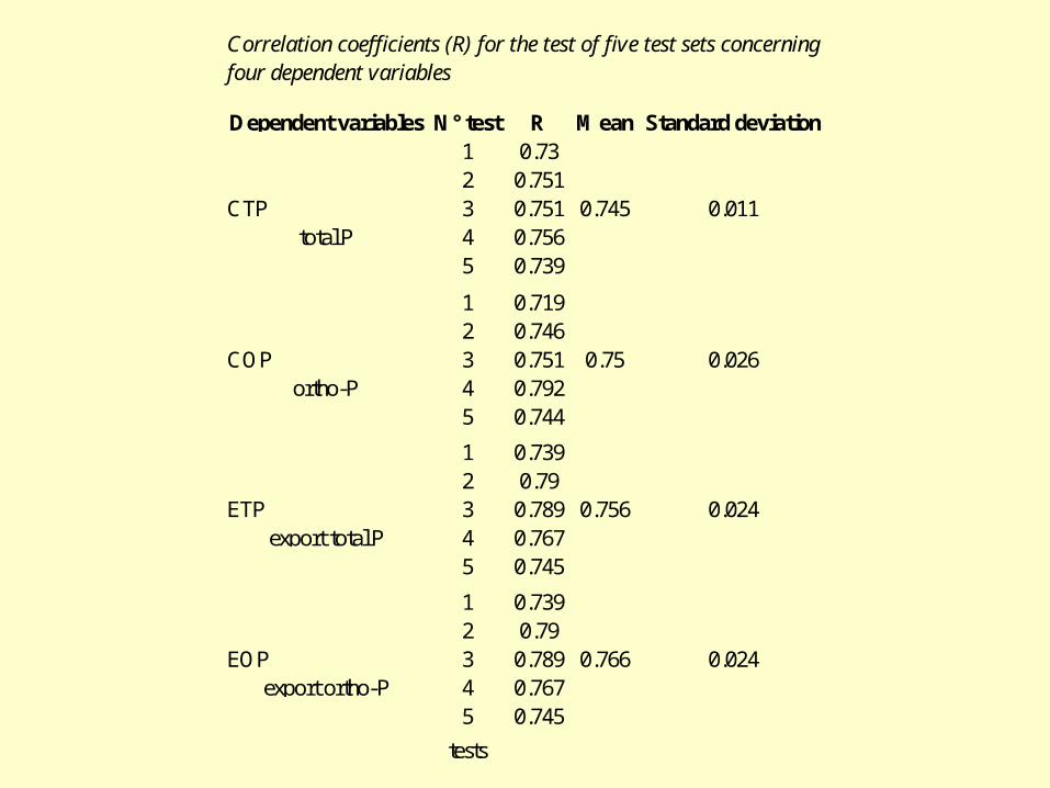
Dependent variables N° test R Mean Standard deviation1 0.732 0.751
CTP 3 0.751 0.745 0.011total P 4 0.756
5 0.739
1 0.7192 0.746
COP 3 0.751 0.75 0.026ortho-P 4 0.792
5 0.744
1 0.7392 0.79
ETP 3 0.789 0.756 0.024export total P 4 0.767
5 0.745
1 0.7392 0.79
EOP 3 0.789 0.766 0.024export ortho-P 4 0.767
5 0.745
tests
Correlation coefficients (R) for the test of five test sets concerning four dependent variables

Variable Type CharacteristicsWi i Wetted width (m2)
ASSG i Area with suitable spawning gravel for trout
per linear meter of river (m2/linear meter)SV i Surface velocity (m/s)
GRA i Water gradient (%)FWi i Flow / width m2/ s/m)D i Mean depth (m)
SDD i Standard deviation of depth (m)BV i Bottom velocity (m/s)
SDBV i Standard deviation of bottom velocity (m/s)VD i Mean speed / mean depth (m/s/m)R/M d Density of trout redds per linear metre of
stream-bed (redds/m)
Habitat variables to study brown trout reproduction (from Delacoste et al., 1993)
i: independent, d: dependent; these independent variables are non-correlated except SV and BV, R = 0.76.
Structure of the neural network used in this study. F1: input layer of neurons comprising as many neurons as variables at the entry of the system; F2: hidden layer of neurons whose number is determined empirically; F3: output layer of neurons with a single neuron corresponding to a single dependent variable.
Lek et al. (1996)
PREDICTION OF BROWN TROUT SPAWNING SITES

PREDICTION OF BROWN TROUT SPAWNING SITES (R/M)
(R/M = density of trout redds per metre of stream-bed)
205 sites Full model R2 No transfor Transform
Stepwise linear regression 4 vars 0.44 0.62
Multiple linear regression 10 vars 0.47 0.63
Neural network 4 vars 0.81 0.74Neural network 10 vars 0.93 0.96

Neural network modelling: variation of the correlation coefficient between observed and estimated values according to the number of neurons of the hidden layer (average value and standard deviation).
Neural network modelling: variation of the sum squared of errors and the correlation coefficient between observed and estimated values according to the number of iterations.

Correlation graphs between observed and estimated values of R/M by different models: (a) multiple regression(MR) with transformed variables; (b) multiple regression (MR) with non-transformed variables; (c) neural network with four independent variables (NN4) with transformed variables; (d) neural network with four independent variables (NN4) with non-transformed variables; (e) neural network with all the independent variables (NN10) with transformed variables; (f) neural network with all the independent variables (NN10) with non-transformed variables.
Lek et al. (1996)

Relationship between residuals and the estimated and observed values of R/M for transformed variable models: a, b: MR: c, d: NN4; e, f: NN10 Lek et al. (1996)

Contribution profile of each independent variable to the prediction of R / M by NN (five variables are only represented here)
No. test NN MRR_learn R_test R_learn
1 0.892 0.862 0.6852 0.914 0.888 0.6853 0.904 0.906 0.694 0.883 0.867 0.6885 0.905 0.906 0.669
Mean 0.9 0.886 0.684
R2 0.81 0.79 0.468
0.6260.566
R_test
0.371
Results of the NN and MR models on random training setfractions (3/4) of the records) and test set fractions (theremaining 1/4 records)
0.740.609
R_learn: correlation coefficient between estimated and observed values of the training sets; R_test: correlation coefficient of thetest sets.
0.4870.628
Cross Validation
Lek et al. (1996)

CLASSIFICATION (= DISCRIMINANT ANALYSIS) AND ARTIFICIAL NEURAL
NETWORKS
Artificial neural networks
Input vectors Output vectors
>1 Predictor 1 or more Responses Regression
>1 Variable 2 or more ClassesDiscriminant
(or 1/0 Responses) analysis

Malmgren & Nordlund (1996) Paleoceanography 11, 503–512
Four distinct volcanic ash zones in late Quaternary sediments of Norwegian Sea.
Zone A B C D Basaltic and Rhyolithic types
8 classes x 9 variables (Na2O, MgO, Al2O3, SiO, K2O, CaO, TiO2, MnO, FeO)
183 samples
DISCRIMINANT ANALYSIS BY NEURAL NETWORKS
R

(A). Diagram showing the general architecture of a 3-layer back propagation network with five elements in the input layer, three neurons in the hidden layer, and two neurons in the output layer. Each neuron in the hidden and output layers receives weighted signals from the neurons in the previous layer. (B) Diagram showing the elements of a single neuron in a back propagation network. In forward propagation, the incoming signals from the neurons of the previous layer (p) are multiplied with the weights of the connections (w) and summed. The bias (b) is then added, and the resulting sum is filtered through the transfer function to produce the activity (a) of the neuron. This is sent on to the next layer or, in the case of the last layer, represents the output. (C) A linear transfer function (left) and a sigmoidal transfer function (right).

Configuration of grains referable to the 4 late Quaternary volcanic ash zones, A through D, in the Norwegian sea described by Sjøholm et al [1991] along first and second canonical variate axes. The canonical variate analysis is based on the geochemical composition of the individual ash particles (nine chemical elements were analyzed: Na2O, MgO, Al2O3, SiO2, K2O, CaO, TiO2, MnO, and FeO). Two types of grains, basaltic and rhyolithic, were distinguished within each zone. This plane, accounting for 98% of the variability among group mean vectors in nine-dimensional space (the first axis represents 95%), distinguishes basaltic and rhyolithic grains. Apart from basaltic grains from zone C, which may be differentiated from such grains from other zones, grains of the same type are clearly overlapping with regard to the geochemical composition among the zones.
4 zonesA B C D
2 typesRhyoliteBasalt
Malmgren & Nordlund (1996)

Changes in error rate (percentages of misclassifications in the test set) for a three-layer back propagation network with increasing number of neurons when applied to training-test set 1 (80:20% training test partition). Error rates were determined for an incremental series of 3, 6, 9, …., 33 neurons in the hidden layer. Error rates were computed as average rates based on ten independent trials with different initial random weights and biases. The error rates represent the minimum error obtained for runs of 300, 600, 900, and up to 9000 epochs. The minimum error rate (9.2%) was obtained for a configuration with 24 neurons in the hidden layer, although there is a major reduction already at nine neurons. Malmgren & Nordlund (1996)

Changes in error rate (percentages of misclassifications) in the training set with increasing number of epochs in the first out of ten trials in training set 1. This network had 24 neurons in the hidden layer, and the network error was monitored over 30 subsequent intervals of 300 training epochs each. During training, the error rate in the training set decreased from 18.5% after 300 epochs to a minimum of 2.1% after 7500 epochs. The minimum error rate in the test set (10.8%) was reached after 3300 epochs.
Malmgren & Nordlund (1996)

CRITERION OF NEURAL NETWORK SUCCESS
ERROR RATE of predictions in independent test set that is not part of the training set.
Cross-validation 5 random test sets 37 particles
Training set 146 particles
Error rate of misclassification (%) for each test setAverage rate of misclassification (%) for five test sets
NETWORK CONFIGURATION & NUMBER OF TRAINING CYCLES
24 neurons
Training set – minimum in error rate
7500 cycles
Test set – minimum in error rate
(10.8%) 3300 cycles
OTHER TECHNIQUES USED
Linear discriminant analysis (LDA)
k-nearest neighbour (= modern analog technique) (=KNN)
Soft independent modelling of close analogy (SIMCA)
(close to PLS with classes)
CONCLUSIONS
Average error rate NN network 9.2%
i.e. 33.6 out of 37 particles correctly classified
LDA 38.4% K-NN 30.8%SIMCA 28.7%

Error rates (percentages of misclassifications in the test sets) for each of the five independent training-test set partitions (80% training set and 20% test set members) and average error rates over the five partitions for a three-layer back propagation (BP) neural network, linear network, linear discriminant analysis, the k-nearest neighbours technique (k-NN) and SIMCA. Neural network results are based on ten independent trials with different initial conditions. Error rates for each test set are represented by the average of the minimum error rates obtained during each of the ten trials, and the fivefold average error rates are the averages of the minimum error rates for the various partitions.

Error rates in each of five training-test set partitions, fivefold average error rates in the test sets, and 95% confidence intervals for the fivefold average error rates for the techniques discussed in this paper.
The fivefold average error rates were determined as the average error rates over five independent training and test sets using 80% training and 20% test partitions. Error rates for the neural networks are averages of ten trials for each training-test set partition using different initial conditions ((random initial weights and biases). The minimum fivefold error rate for the back propagation (BP) network was obtained using 24 neurons in the hidden layer. Apart from regular error rates for soft independent modelling of class analogy (SIMCA 1), the total error rates for misclassified observations that could be referable to one or several other groups are reported under SIMCA 2. LDA represents linear discriminant analysis and k-NN, k-nearest neighbour.
Neural N

Average error rates (percentages) for basaltic and rhyolithic particles in ash zones A through D
As before, error average error rates over five experiments based on 80% training set members and 20% test set members. N is the range of sample sizes in these experiments.

As in the use of ANN in regression, problems of over-fitting and over-training and reliable model testing occur. n-fold cross-validation needed with an independent test set (10% of observations), an optimisation data set (10%), and a training or learning set (80%). Repeated n-times (usually 10).
ANN a computationally slow way of implementing two- or many-group discriminant analysis. No obvious advantages.
Allows use of 'mixed' data about groups (e.g. continuous, ordinal, qualitative, presence/absence). But can use mixed data in canonical analysis of principal co-ordinates if use the Gower coefficient for mixed data.

Malmgren & Nordlund, 1996. Palaeoceanography 11, 305-512 (volcanic ash discriminant analysis)
Malmgren & Nordlund, 1997. Palaeo, Paleao, Palaeo 136, 359-373 (surface temperature reconstructions)
Lek et al., 1996. Ecological Modelling 90, 39-52 (trout & habitat regression)
Lek et al., 1996. Acta Oecologia 17, 43-53 (phosphorus & land-use)
Mastrorillo et al., 1997. Freshwater Biology 38, 237-246 (fish +/- and habitats)
Borggaard & Theoberg, 1992. Annl. Chem. 64, 545-551 (near infra-red spectra)
Whitehead et al., 1997. Hydrobiologia 349, 47-57 (blue-green algae)
Poff, Tokar & Johnson, 1996. Limnology & Oceanography 41, 857-863 (stream hydrology)
Guegan et al., 1998. Nature 391, 382-384 (fish diversity)
Racca et al., 2001. J. Paleolimnology 26, 411-422 (diatoms & pH)
Malmgren et al., 2001. Paleoceanography 16, 520-530 (forams & sea temperatures)
Peyron & de Vernal, 2001. J. Quaternary Science 16, 699-709 (dinoflagellates & sea temperatures)
NEURAL NETWORK APPLICATIONS

REGRESSION MODELS AS PREDICTIVE TOOLS
(1) presence/absence of 27 fish species as a function of 13 habitat features in 286 temperate lakes
(2) Monte Carlo simulated presence/absence data with a range of deterministic, linear, and non-linear species responses (30 samples x 500 times)
Olden & Jackson (2002) Freshwater Biology 47, 1976-1995
Compared logistic regression analysis, linear discriminant analysis, classification trees, and artificial neural networks to predict:
(Regression models mainly concerned with descriptive and explanatory roles.)
Criteria of prediction performance:
(i) Percentage of lakes where presence or absence of species correctly classified
(ii) Ability to predict species presence (sensitivity) correctly
(iii) Ability to predict species absence (specificity) correctly

RESULTS
(i) Real data (ii) Simulated data
(iii) On average, neural networks outperformed the other methods but for species presence/absence all methods showed moderate to excellent success.
(Correct classification 80-85%, specificity 70-75%, sensitivity 35-75%)
Neural networks consistently had best performance.
(iv) Simulated non-linear data – neural networks (98% correct) and classification trees (89% correct) greatly outperformed other methods.
(v) Simulated linear data. All methods good (92-100% correct).
Classification trees and neural networks have the advantage that they can model both linear and non-linear responses; linear discriminant analysis poor with non-linear data; logistic regression surprisingly poor with non-linear data.

A Warning About Artificial Neural Network Software
Telford et al. 2004 Palaeoceanography 19, PA4014, doi: 10.1029/2004PA001072
ANN are algorithms that by mimicking biological neural networks have the ability to learn by example. Learn by iteratively adjusting a large set of parameters (originally set at random values) to minimise the error between the predicted output and actual input.
If trained for too long, ANNs can over-fit the data by learning particular features of the data rather than learning the general rules.

Need to have
(1) modelling data-set
(2) independent optimisation data-set and, when training and optimisation are done,
(3) independent test-set
Not all software makes the distinction between (2) and (3), and some use (2) as a test-set.
When a truly independent test-set is used, ANN does not out-perform more 'classical' methods.
Not always clear from published studies what was done.
Be cautious when reading about the fantastic performance of ANN

ANN CONCLUSIONS
ANN are, if used carefully, a flexible class of non-linear regression models. By adding more hidden layers, can control complexity of model from relatively simple models to models with complex structure.
Seem attractive because they require less expertise to use compared to GLM, etc. BUT users must pay attention to basic statistical issues of transformations, scalings, outliers, influential points, and minimal adequate models.
May be good for prediction but bad for understanding. The ANN weights are almost un-interpretable. ANN usually introduce complex interactions that often do not reflect reality.
Easy to over-fit, giving over-optimistic predictions.
No statistical theory for inference, diagnostics, or model selection.
ANN are, at best, a tool; not a rigorous method with underlying theory.

Generalised Linear ModelsSYSTAT GLIMGENSTATS-PLUSR
Generalised Additive ModelsGAIMGENSTATS-PLUSR
SOFTWARE FOR ADVANCED OR MODERN REGRESSION ANALYSIS
Locally Weighted Regression & SplinesSYSTAT GENSTAT S-PLUSR
Classification & Regression TreesSYSTAT S-PLUSCARTR
Neural NetworksMATLAB Neural Network ToolboxS-PLUS (Functions) NGO Neuro-Genetic OptimiserR (Libraries)