lecture 42: review of active mosfet circuits

Department of EECS University of California, Berkeley

EECS 105 Fall 2004, Lecture 42

Lecture 42: Review of active MOSFET circuits

Prof. J. S. Smith


EECS 105 Spring 2004, Lecture 42 Prof. J. S. Smith

Final Exam

Covers the course from the beginning Date/Time: SATURDAY, MAY 15, 2004 8-11A Location: BECHTEL auditorium One page (Two sides) of notes



Observed Behavior: ID-VDS

For low values of drain voltage, the device is like a resistor As the voltage is increases, the resistance behaves non-linearly

and the rate of increase of current slows Eventually the current stops growing and remains essentially

constant (current source)

DSV

/DSI k

“constant” current

resistor region

non-linear resistor region

2GSV V

3GSV V

4GSV V

GSV

DSIDSV



Observed Behavior: ID-VDS

DSV

/DSI k

“constant” current

resistor region

non-linear resistor region

2GSV V

3GSV V

4GSV V

GSV

DSIDSV

As the drain voltage increases, the E field across the oxide at the drain endis reduced, and so the charge is less, and the current no longer increases proportionally. As the gate-source voltage is increased, this happensat higher and higher drain voltages. The start of the saturation region is shaped like a parabola



Finding ID = f (VGS, VDS)

Approximate inversion charge QN(y): drain is higher than the source less charge at drain end of channel



Inversion Charge at Source/Drain

)(

)0(

TnGSox

N

VVC

yQ

)( LyQN

)( TnGDox VVC

DSGSGD VVV

2

)()0()(

LyQyQyQ NN

N

The charge under the gate along the gate, but we are going to make a simple approximation, that the average charge is the average of the charge near the source and drain



Average Inversion Charge

Charge at drain end is lower since field is lower Notice that this only works if the gate is inverted along its

entire length If there is an inversion along the entire gate, it works well

because Q is proportional to V everywhere the gate is inverted

( ) ( )( )

2ox GS T ox GD T

N

C V V C V VQ y

Source End Drain End

( ) ( )( )

2ox GS T ox GS SD T

N

C V V C V V VQ y

(2 2 )( ) ( )

2 2ox GS T ox SD DS

N ox GS T

C V V C V VQ y C V V



Drift Velocity and Drain Current

“Long-channel” assumption: use mobility to find v

( ) ( ) ( / ) n DSn n

Vv y E y V y

L

And now the current is just charge per area, times velocity, times the width:

( )2

DS DSD N ox GS T

V VI WvQ W C V V

L

( )2DS

D ox GS T DS

VWI C V V V

L

Inverted Parabolas



Square-Law Characteristics

Boundary: what is ID,SAT?TRIODE REGION

SATURATION REGION



The Saturation Region

When VDS > VGS – VTn, there isn’t any inversioncharge at the drain … according to our simplistic model

Why do curvesflatten out?



Square-Law Current in Saturation

Current stays at maximum (where VDS = VGS – VTn )

Measurement: ID increases slightly with increasing VDS

model with linear “fudge factor”

( )2DS

D ox GS T DS

VWI C V V V

L

, ( )( )2

GS TDS sat ox GS T GS T

V VWI C V V V V

L

2, ( )

2ox

DS sat GS T

CWI V V

L

2, ( ) (1 )

2ox

DS sat GS T DS

CWI V V V

L



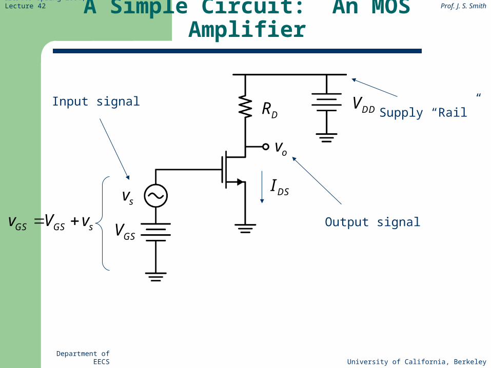
A Simple Circuit: An MOS Amplifier

DSI

GSV

sv

DR DDV

GS GS sv V v

ov

Input signal

Output signal

Supply “Rail”



Small Signal Analysis

Step 1: Find DC operating point. Calculate

(estimate) the DC voltages and currents (ignore

small signals sources)

Substitute the small-signal model of the

MOSFET/BJT/Diode and the small-signal models

of the other circuit elements.

Solve for desired parameters (gain, input

impedance, …)



A Simple Circuit: An MOS Amplifier

DSI

GSV

sv

DR DDV

GS GS sv V v

ov

Input signal

Output signal

Supply “Rail”



Small-Signal Analysis

Step 1. Find DC Bias – ignore small-signal source

VGS,BIAS was found inLecture 15

IGS,Q



Small-Signal Modeling

What are the small-signal models of the DC supplies?

Shorts!



Small-Signal Models of Ideal Supplies

Small-signal model:

supplysupply

supply

ig

v

supply 0r

supplysupply

supply

0i

gv

supplyr

short

open



Small-Signal Circuit for Amplifier



Low-Frequency Voltage Gain

Consider first 0 case … capacitors are open-circuits

Transconductance

,2( ) D SAT

m n ox GS TGS T

IWg C V V

L V V

||out m s D ov g v R r

||v m D oA g R r

Design Variable

Design Variables



Voltage Gain (Cont.)

Substitute transconductance:

Output resistance: typical value n= 0.05 V-1

,

1 1200k

0.05 0.1on D SAT

r kI

Voltage gain: 2 0.125 || 200 14.3

0.32vA

,2||D SAT

v D oGS T

IA R r

V V

m Dg R



Input and Output Waveforms

Output small-signal voltage amplitude: 14 x 25 mV = 350

Input small-signal voltage amplitude: 25 mV



What Limits the Output Amplitude?

1. vOUT(t) reaches VSUP or 0 … or

2. MOSFET leaves constant-current region and enters triode region

, 0.31VDS DS SAT GS TnV V V V

, , 0.32Vo MIN DS SATv V

2.5 0.32V = 2.18Vamp



Maximum Output Amplitude

vout(t)= -2.18 V cos(t) vs(t) = 152 mV cos(t)

How accurate is the small-signal (linear) model?

0.1520.5

0.32s

GS Tn

v

V V

Significant error in neglecting third term in expansion of iD = iD (vGS)



One-Port Models (EECS 40)

A terminal pair across which a voltage and associated current are defined

CircuitBlockabv

abi

thevv

thevR

abv

abi

thevithevRabv

abi



Small-Signal Two-Port Models

We assume that input port is linear and that the amplifier is unilateral: – Output depends on input but input is independent of

output. Output port : depends linearly on the current and

voltage at the input and output ports Unilateral assumption is good as long as “overlap”

capacitance is small (MOS)

inv

outv

outiini



Two-Port Small-Signal Amplifiers

si sR inR outR LRi inAi

ini

sv

sR

inR

outR

LRv inA vinv

Current Amplifier

Voltage Amplifier



Two-Port Small-Signal Amplifiers

sv

sR

inRoutR LRm inG v

inv

si sR inR

outR

LRm inR i

ini

Transresistance Amplifier

Transconductance Amplifier



Common-Source Amplifier (again)

How to isolate DC level?



DC Bias

Neglect all AC signals

5 V

2.5 V

Choose IBIAS, W/L



Load-Line Analysis to find Q

Q

D

DD outR

D

V VI

R

1

10kslope

0V

10kDI

5V

10kDI



Small-Signal Analysis

inR



sv

sR

inRoutR LRm inG v

inv

Two-Port Parameters:

Find Rin, Rout, Gm

inR

m mG g ||out o DR r R

Generic Transconductance Amp



Two-Port CS Model

Reattach source and load one-ports:



Maximize Gain of CS Amp

Increase the gm (more current) Increase RD (free? Don’t need to dissipate extra power) Limit: Must keep the device in saturation

For a fixed current, the load resistor can only be chosen so large To have good swing we’d also like to avoid getting too close to saturation

||v m D oA g R r

,DS DD D D DS satV V I R V



Current Source Supply

Solution: Use a current source!

Current independent of voltage for ideal source



CS Amp with Current Source Supply



Load Line for DC Biasing

Both the I-source and the transistor are idealized for DC bias analysis



Two-Port Parameters

From currentsource supply

inR

||out o ocR r r

m mG g



P-Channel CS Amplifier

DC bias: VSG = VDD – VBIAS sets drain current –IDp = ISUP



Common Gate Amplifier

DC bias:

SUP BIAS DSI I I

current gain=1Impedance buffer

Gain of transistortends to hold this node at ss ground:low input impedanceload for current input

Notice that IOUT must equal-Is



CG as a Current Amplifier: Find Ai

out d ti i i

1iA



CG Input Resistance

At input:

Output voltage:

t outt m gs mb t

o

v vi g v g v

r

( || ) ( || )out d oc L t oc Lv i r R i r R

gs tv v

||t oc L tt m t mb t

o

v r R ii g v g v

r



Approximations…

We have this messy result

But we don’t need that much precision. Let’s start approximating:

1

1||

1

m mbt o

oc Lin t

o

g gi r

r RR vr

1m mb

o

g gr

||oc L Lr R R 0L

o

R

r

1in

m mb

Rg g



CG Output Resistance

( ) 0s s tm gs mb s

S o

v v vg v g v

R r

1 1 ts m mb

S o o

vv g g

R r r



CG Output Resistance

Substituting vs = itRS

1 1 tt S m mb

S o o

vi R g g

R r r

The output resistance is (vt / it)|| roc

|| 1oout oc S m o mb o

S

rR r R g r g r

R



Approximating the CG Rout

The exact result is complicated, so let’s try tomake it simpler:

Sgm 500 Sgmb 50 kro 200

][|| SSombSomoocout RRrgRrgrrR

][|| SSomoocout RRrgrrR

Assuming the source resistance is less than ro,

)]1([||][|| SmoocSomoocout RgrrRrgrrR



CG Two-Port Model

Function: a current buffer

•Low Input Impedance•High Output Impedance



Common-Drain Amplifier

21( )

2DS ox GS T

WI C V V

L

2 DSGS T

ox

IV V

WC

L

Weak IDS dependence

In the common drain amp,the output is taken from aterminal of which the currentis a sensitivefunction



CD Voltage Gain

Note vgs = vt – vout

||out

m gs mb outoc o

vg v g v

r r

||

outm t out mb out

oc o

vg v v g v

r r



CD Voltage Gain (Cont.)

KCL at source node:

Voltage gain (for vSB not zero):

||

outm t out mb out

oc o

vg v v g v

r r

1

|| mb m out m toc o

g g v g vr r

1||

out m

inmb m

oc o

v g

v g gr r

1out m

in mb m

v g

v g g



CD Output Resistance

Sum currents at output (source) node:

|| || tout o oc

t

vR r r

i t m t mb ti g v g v

1out

m mb

Rg g



CD Output Resistance (Cont.)

ro || roc is much larger than the inverses of the transconductances ignore

1out

m mb

Rg g

Function: a voltage buffer•High Input Impedance•Low Output Impedance



Voltage and current gain

Current tracks input

voltage tracks input



Bias sensitivity

When a transistor biasing circuit is designed, it is important to realize that the characteristics of the transistor can vary widely, and that passive components vary significantly also.

Biasing circuits must therefore be designed to produce a usable bias without counting on specific values for these components.

One example is a BJT base bias in a CE amp. A slight change in the base-emitter voltage makes a very large difference in the quiescent point. The insertion of a resistor at the emitter will improve sensitivity.



Insensitivity to transistor parameters

Most of the circuit parameters are independent of variation of the transistor parameters, and depend only on resistance ratios. That is often a design goal, but in integrated circuits we will not want to use so many resistors.



NMOS pullup

Rather than using a big (and expensive) resistor, let’s look at a NMOS transistor as an active pullup device

Note that when the transistor is connected this way, it is not an amplifier,it is a two terminal device. When the gate is connected to the drain of this NMOS device, it will be in saturation, so we get the equation for the drain current:

SDnTnSGoxnD VVVCL

WI

1

22

+V

outv



Small signal model

So we have:

The N channel MOSFET’s transconductance is:

And so the small signal model for this device will be a resistor with a resistance:

22

2

21

2

12

TnoxnnTnoxn

SDnTnSGoxnD

VVCL

WVVVC

L

W

VVVCL

WI

DoxnTnSGoxn

Q

DSG

m ICL

WVVC

L

Wi

vg

2

mgr

1



IV for NMOS pull-up

The I-V characteristic of this pull-up device:

21 TnDDoxnD VVC

L

WI

2tDD VV I

VDDV



Active Load We can use this as the pullup device for an NMOS common

source amplifier:

inv

outv

2111

11 2 TngsoxnD VVC

L

WI

2222

22 2 TngsoxnD VVC

L

WI

DDV

20 gsDD VVV

22

220 /

2

LWC

IVVV

oxntDD

2M

1M



Active LoadSince I2=I1 we have:

inv

outv

DDV 22

120 /

2

LWC

IVVV

oxntDD

And since: igs VV 1

1

22

1110 /

/titnDD VV

LW

LWVVV

2M

1M



Behavior

If the output voltage goes higher than one threshold below VDD, transistor 2 goes into cutoff and the amplifier will clip.

If the output goes too low, then transistor 1 will fall out of the saturation mode.

Within these limitations, this stage gives a good linear amplification.



CMOS Diode Connected Transistor

Short gate/drain of a transistor and pass current through it

Since VGS = VDS, the device is in saturation since VDS > VGS-VT

Since FET is a square-law (or weaker) device, the I-V curve is very soft compared to PN junction diode



Diode Equivalent Circuit

1

0OUT

OUT tD

OUT tI

di vR

dv i

Equivalent Circuit:

RD

+ -

iOUT

+

-

VD vOUT

1D

m

Rg



The Integrated “Current Mirror” M1 and M2 have the same

VGS

If we neglect CLM (λ=0), then the drain currents are equal

Since λ is small, the currents will nearly mirror one another even if Vout is not equal to VGS1

We say that the current IREF is mirrored into iOUT

Notice that the mirror works for small and large signals!

High Res

Low Resis



Current Mirror as Current Sink

The output current of M2 is only weakly dependent on vOUT due to high output resistance of FET

M2 acts like a current source to the rest of the circuit



Small-Signal Resistance of I-Source



Improved Current Sources

Goal: increase roc Approach: look at amplifier output resistance results … to see topologies that boost resistance

Looks like the output impedance of a common-source amplifier with source degeneration

out oR r



Effect of Source Degeneration

Equivalent resistance loading gate is dominated by the diode resistance … assume this is a small impedance

Output impedance is boosted by factor

( )St t m gs o Rv i g v r v

1eq

m

Rg

Sgs Rv v

SR t Sv i R

( )t t m S t o t Sv i g R i r i R

1to m S o

t

vR g R r

i

1 m Sg R



Cascode (or Stacked) Current Source

Insight: VGS2 = constant AND VDS2 = constant

Small-Signal Resistance roc:

1o m S oR g R r

1o m o oR g r r

20o m oR g r r



Drawback of Cascode I-Source

Minimum output voltage to keep both transistors in saturation:

, 4, 2,OUT MIN DS MIN DS MINV V V

vOUT

iOUT

2, 2 0 2DS MIN GS T DSATV V V V

4 2 4 2 4 0D DSAT GS GS GS TV V V V V V

, 2 4 0OUT MIN GS GS TV V V V



Current Sinks and Sources

Sink: output current goes to ground

Source: output current comes from voltage supply



Current Mirrors

We only need one reference current to set up all the currentsources and sinks needed for a multistage amplifier.



Summary of Cascaded Amplifiers

General goals:

1. Boost the gain (except for buffers)2. Improve frequency response3. Optimize the input and output resistances:

Rin Rout

Voltage:

Current:

Transconductance:

Transresistance:

00

0 0



Start: Two-Stage Voltage Amplifier

• Use two-port models to explore whether the combination “works”

CS1CS2

Results of new 2-port: Rin = Rin1, Rout = Rout2

1 2 1 2 2||v m in out m outA G R R G R

1 2 2 1 2||v m m in out outA G G R R R

CS1,2



Cascading stages

CS1CS2 CD3

Output resistance:

Voltage gain (2-port parameter):

Input resistance:

1 1 1 2 2 2|| ||v m o oc m o ocA g r r g r r

1out

m mb

Rg g

lecture 42: review of active mosfet circuits

Documents