Lecture 3

Central Tendency And Variability

Central Tendency Central tendency = statistical measure that

identifies a single score as representative of an entire distribution. – Median – Mean– Mode

MORE ABOUT DISTRIBUTIONS - Measures of central tendency help us to summarize and understand the distribution better

** The important thing to remember about central tendency is that these measures describe and summarize a group of individuals rather than any single person. IN FACT, the average person may not exist!

Distributions: Try to Find the “Center”

f

1 2 3 4 5 6 7 98

f

1 2 3 4 5 6 7 98

f

1 2 3 4 5 6 7 98

The Mean Arithmetic Average: computed by adding all

scores in the distribution and dividing by the number of scores.

Population mean = , Greek letter mu

Sample mean = M or X, read “x-bar”

Computed:

= X / N M = X / n

Conceptualizing the Mean

The amount each individual would get if the total (X) were divided equally amongst the individuals (n)– 10 friends plan to pitch in for lotto tickets. They

want to buy $200 dollars worth of tickets. What is the average amount each person would have to put in? X = 200, n = 10, so M = ?

– The friends are lucky and won the jackpot. They each got a share of 500 K. Given this information what is the total amount of money won?

• M = 500 K, n = 10, X = ?

M = X / n

Conceptualizing the Mean

A balance point for a distribution… Consider a population consisting of N scores:2, 4, 8, 10

Balance by distance Always must occur between hi and low score

= X / N

1 2 3 4 5 6 7 8 9 10

Score Distance from

X=2 4 pts below M

X=4 2 pts below M

X=9 3 pts above M

X=9 3 pts above M

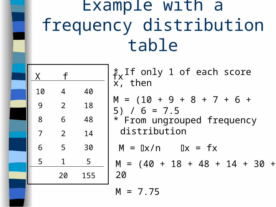
Example with a frequency distribution table

X f fx

10

9

8

7

6

5

4

2

6

2

5

1

20

40

18

48

14

30

5

155

* If only 1 of each score x, then

M = (10 + 9 + 8 + 7 + 6 + 5) / 6 = 7.5

* From ungrouped frequency distribution

M = x/n x = fx

M = (40 + 18 + 48 + 14 + 30 + 5) / 20

M = 7.75

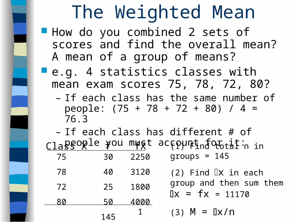
The Weighted Mean How do you combined 2 sets of scores and

find the overall mean? A mean of a group of means?

e.g. 4 statistics classes with mean exam scores 75, 78, 72, 80?– If each class has the same number of people: (75

+ 78 + 72 + 80) / 4 = 76.3– If each class has different # of people you must

account for it:Class X f fX

75

78

72

80

30

40

25

50

145

2250

3120

1800

40001

11170

(1) Find total n in groups = 145

(2) Find x in each group and

then sum them x = fx = 11170

(3) M = x/n

M = 11170/ 145 = 77

An alternative procedureClass X f fX

75

78

72

80

30

40

25

50

145

2250

3120

1800

40001

11170

M = (30/145)(75) + (40/145)(78) + (25/145)(72) + (50/145)(80)

M = .21(75) + .28(78) + .17(72) + .34(80)

M = 15.75 + 21.84 + 12.24 + 27.2

M = 77.03

* For yet another way to compute weighted means see Box 3.1 in your book (pg. 77).

Characteristics of the Mean Most commonly used measure of central

tendency– Because it uses every score in the distribution it

tends to be a good representative May or may not be an occurring score Very sensitive to outliers

– e.g. 1, 3, 4, 5, 5, 6, 10, 100 (M = 16.75) Affected by skewed distributions - pulled

toward the extremes Closely related to the variance and standard

deviation…makes it good for use with inferential statistics– Summed deviations = 0 (more on this later)

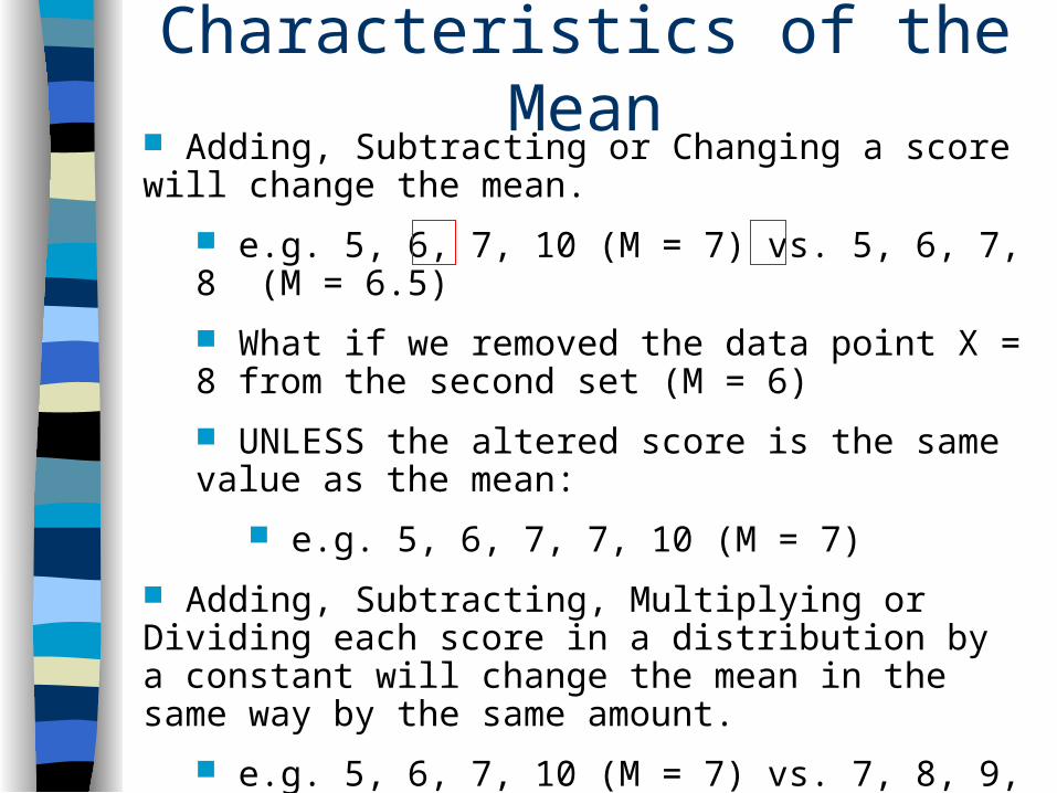
Adding, Subtracting or Changing a score will change the mean.

e.g. 5, 6, 7, 10 (M = 7) vs. 5, 6, 7, 8 (M = 6.5)

What if we removed the data point X = 8 from the second set (M = 6)

UNLESS the altered score is the same value as the mean:

e.g. 5, 6, 7, 7, 10 (M = 7)

Adding, Subtracting, Multiplying or Dividing each score in a distribution by a constant will change the mean in the same way by the same amount.

e.g. 5, 6, 7, 10 (M = 7) vs. 7, 8, 9, 12 (M = 9)

e.g. 5, 6, 7, 10 (M = 7) vs. 10, 12, 14, 20 (M = 14)

Characteristics of the Mean

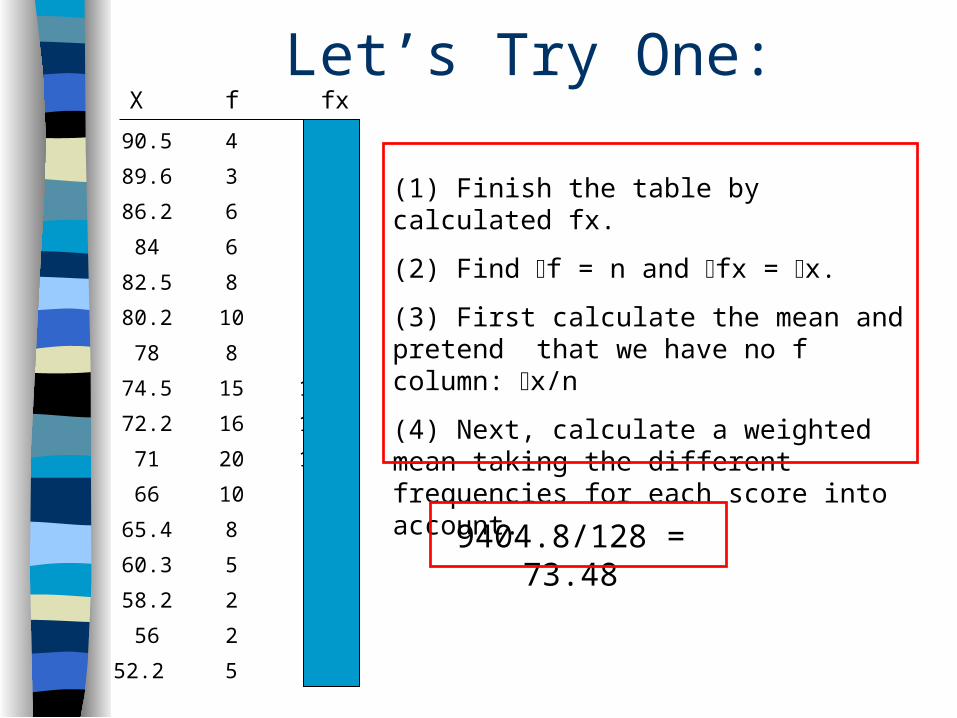
Let’s Try One:X f fx

(1) Finish the table by calculated fx.

(2) Find f = n and fx = x.

(3) First calculate the mean and pretend that we have no f column: x/n

(4) Next, calculate a weighted mean taking the different frequencies for each score into account.

90.5 4 362

89.6 3 269

86.2 6 517

84 6 504

82.5 8 660

80.2 10 802

78 8 624

74.5 15 1118

72.2 16 1155

71 20 1420

66 10 660

65.4 8 523

60.3 5 302

58.2 2 116

56 2 112

52.2 5 261

9404.8/128 = 73.48

Admin wants to know the mean grade for all stats classes for the year 2003-2004 at the UA. Below are the mean grades and the number of people in the class.

Grade Class size fx

75 34 2550

80 42 3360

82 200 16400

68 156 10608

88 75 6600

77 222 17094

72 144 10368

83 172 14276

81256/1045 =

77.76

The Median

Median - Divides the distribution into exactly 2 parts (by area). The median is equal to PR 50.

No sanctioned abbreviation for the median; some use Mdn.

The definition and computations for the median are identical for populations and samples.

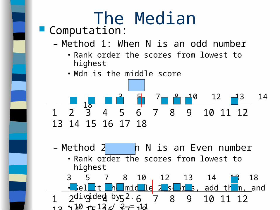
Computation:– Method 1: When N is an odd number

• Rank order the scores from lowest to highest• Mdn is the middle score

3 5 7 8 10 12 13 14 18

– Method 2: When N is an Even number• Rank order the scores from lowest to highest3 5 7 8 10 12 13 14 18 18 • Select the middle 2 scores, add them, and divided by 2.• 10 + 12 / 2 = 11

The Median

1 2 3 4 5 6 7 8 9 10 11 12 13 14 15 16 17 18

1 2 3 4 5 6 7 8 9 10 11 12 13 14 15 16 17 18

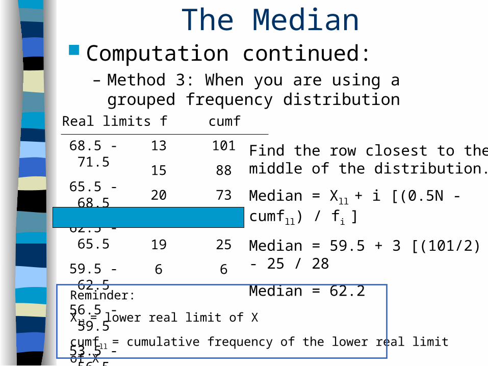
The Median Computation continued:

– Method 3: When you are using a grouped frequency distribution

Real limits f cumf

68.5 - 71.5

65.5 - 68.5

62.5 - 65.5

59.5 - 62.5

56.5 - 59.5

53.5 - 56.5

13

15

20

28

19

6

101

88

73

53

25

6

Find the row closest to the middle of the distribution.

Median = Xll + i [(0.5N - cumfll) / fi ]

Median = 59.5 + 3 [(101/2) - 25 / 28

Median = 62.2

Reminder:

Xll = lower real limit of X

cumfll = cumulative frequency of the lower real limit of X

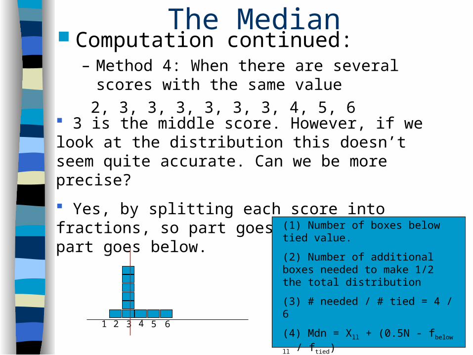
The Median Computation continued:

– Method 4: When there are several scores with the same value

2, 3, 3, 3, 3, 3, 3, 4, 5, 6

3 is the middle score. However, if we look at the distribution this doesn’t seem quite accurate. Can we be more precise?

Yes, by splitting each score into fractions, so part goes above the mdn and part goes below.

(1) Number of boxes below tied value.

(2) Number of additional boxes needed to make 1/2 the total distribution

(3) # needed / # tied = 4 / 6

(4) Mdn = Xll + (0.5N - fbelow ll / ftied)

Mdn = 2.5 + (5 - 1 / 6) = 3.17

1 2 3 4 65

Characterizing the Median Will be an occurring score with a odd N Not affected by outliers Not affected by skewed distributions Will likely change with addition of scores Good for distributions that are truncated, open-ended

or missing data (can’t calculate a mean under these conditions)– Truncated: only part of the distribution is being used– Open-ended: top or bottom category has only 1 limit

• E.g. score of 70 or more • Or < 50

– Missing data: data missing due to drop out or incompletion

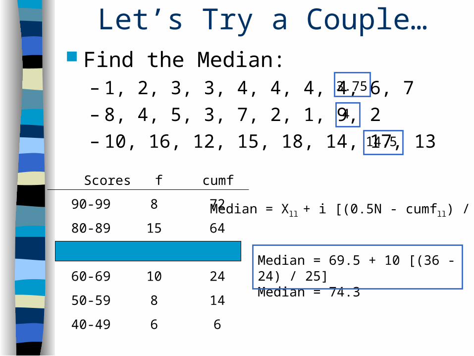
Let’s Try a Couple… Find the Median:

– 1, 2, 3, 3, 4, 4, 4, 4, 6, 7– 8, 4, 5, 3, 7, 2, 1, 9, 2– 10, 16, 12, 15, 18, 14, 17, 13

Scores f cumf

90-99

80-89

70-79

60-69

50-59

40-49

8

15

25

10

8

6

72

64

49

24

14

6

Median = Xll + i [(0.5N - cumfll) / fi ]

Median = 69.5 + 10 [(36 - 24) / 25]Median = 74.3

4

14.5

3.75

Reconceptualizing the Middle: The Mean vs. The Median

f

2 4 6 8 10 12 14 1816

= 12 for N = 12 [balanced by distance: 4+4+6+6+6 (26) above the mean and 2+2+4+4+4+4+6 (260 below the mean]

Median = 10 (6 boxes on either side…balanced by area)

The Mode Mode = the most common observation among

a group of scores. Highest frequency score. Like median no special symbols to denote the mode.

Also, no separate definition for pop. v. sample. Computations:

– 1, 3, 4, 6, 7, 7, 7, 9, 9 mode = 7– 1, 2, 2, 2, 3, 4, 4, 9, 9, 9 mode = 2, 9

– It is possible to have more than one mode. • 2 modes = bi-modal• N modes = multimodal• Lots and lots scores with equal high points = NO mode

Class f68.5 - 71.5

65.5 - 68.5

62.5 - 65.5

10

16

9

(1) Find highest f value

(2) Report midpoint as mode

mode = (65.5 + 68.5) / 2 = 67

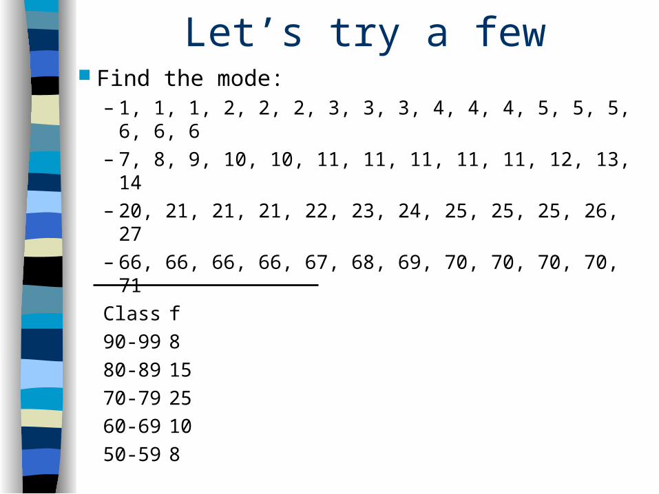
Let’s try a few Find the mode:

– 1, 1, 1, 2, 2, 2, 3, 3, 3, 4, 4, 4, 5, 5, 5, 6, 6, 6– 7, 8, 9, 10, 10, 11, 11, 11, 11, 11, 12, 13, 14– 20, 21, 21, 21, 22, 23, 24, 25, 25, 25, 26, 27– 66, 66, 66, 66, 67, 68, 69, 70, 70, 70, 70, 71

Class f

90-99 8

80-89 15

70-79 25

60-69 10

50-59 8

Characterizing the Mode Will be an occurring score (except possibly

with a grouped frequency distribution).

May or may not change with the addition of scores.

Not sensitive to outliers.

Affected by skewed distributions - pushed away from extremes.

Which to Use? Mean - Most common…great for normal

distributions. Interval or Ratio data. Median - Good for use with:

-- skewed -- truncated -- open-ended -- missing data -- ordinal data

Mode - Quick and dirty, but crude. Can have multiple modes. Good for use with:

-- discrete data-- nominal scale

-- shape

Symmetrical Distributions* In all distributions:

Mode= tallest point

Median = middle point in area

Mean = balancing point

Normal Distribution: symmetrical

unimodal, and asymptotic

mode mean and median

mean and median

No mode

Positively Skewed Distribution

Mode < Mean < Mean

* Note the Mean is most affected by outliers or skewed distributions

Negatively Skewed Distributions

Mean < Median < Mode

Group ActivityYou are planning on buying a car. At this

point, you have narrowed it down to three models (A, B, & C) all from the same year. All factors are equivalent except MPG. To help you decide, the dealer tells you that she can provide one measure of central tendency, the same measure, for each model’s MPG. Which measure would you choose to know? Why?

Variability

• Variability provides a quantitative measure of the degree to which scores in a distribution are spread out of clustered together

Why is Variability Important? Variability defines the spread of a distribution

in terms of distance. Are scores close together? Are they far apart?

Measures how well an individual score (or group of scores) represents an entire population. This has important implications for research!!– So, variability provides a measure of how much

error to expect if you are using a sample to represent a population

Central tendency and variability are closely related. The more you understand their relationship, the better you will understand statistics.

Class A Class B

If you randomly select an individual grade from each of these distributions which individual A or B will more closely represent the entire distribution?

Measures of Variability

Range

Interquartile range and Semi-Interquartile range

Standard Deviation and Variance

Range Difference between the largest and

smallest value in a distribution= Upper real limit - Lower real limit = OR hi - lo +1

Can increase with the addition of scores Cannot decrease with the addition of

scores Find the range of:

{1, 1, 1, 2, 5, 100 } & {1, 25, 50, 77, 80, 100}

Various types including percentiles & quartiles

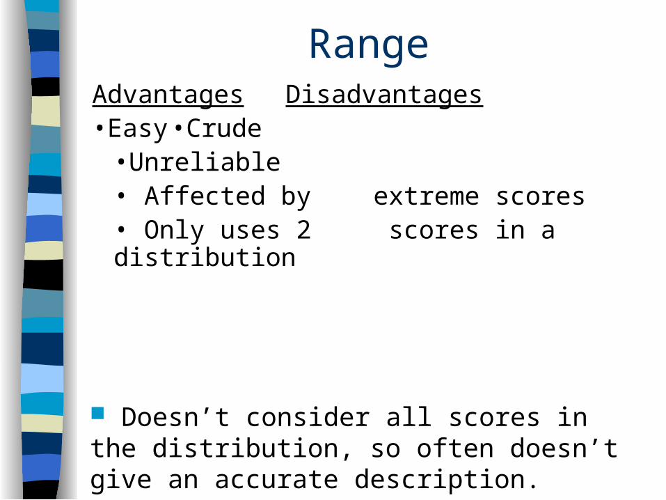
RangeAdvantages Disadvantages•Easy •Crude

•Unreliable• Affected by extreme scores• Only uses 2 scores in a distribution

Doesn’t consider all scores in the distribution, so often doesn’t give an accurate description.

Percentiles

Reminder that percentiles can be one way of looking at a distribution

Values that divide a distribution into hundredths

Define below where a certain percentage of scores fall– 95th percentile = 95% of the scores are

equal to or fall below this point

Quartiles

Values that divide a distribution into fourths

Quartiles are specifically labeled:– Q1 = 25th percentile

– Q2 = 50th percentile (Median)

– Q3 = 75th percentile

A Special Case: Interquartiles and Semi-Interquartiles

The interquartile range: the middlemost 50% of the distribution= Q3 - Q1

While ranges, in general, are affected by extreme scores, the interquartile range is not (we hacked off the extreme scores)

Because of its relationship with the median, it can be used with ordinal data. (Median = Q2 = 50%)

Semi-Interquartile range = simply 1/2 of the interquartile range = (Q3 - Q1) / 2– Conceptually this measure the distance from the

middle of the distribution to each of the boundaries defining the middle 50%

Computing Quartiles

Use the formulas or interpolation to identify the percentile rankings

OR Use a frequency distribution histogram

f

1 2 3 4 5 6 7 98

Q1=3.5 Q3=7

Interquartile range is 3.5 points

Semi-interquartile range = 1.75

Interquartile and Semi-Interquartile range

Advantages Not affected by

outliers Can be used with

skewed distributions Can be used with

ordinal data

Disadvantages Throws away too

much data

Example For the following data set compute the

range, the interquartile range, and the semiquartile range

1, 2, 2, 3, 6, 10, 12, 12, 13, 14, 15, 20, 20, 18, 21, 17

Standard Deviation

The average distance from the mean…generally far or near?

This is the most commonly used and most important measure of variability.

It’s going to tell us how much a score varies from the mean.– Distance of each score from the mean.

Homework - Chapter 3

5, 8, 9, 10, 12, 15, 21, 22, 23, 24

Read IN THE LITERATURE pages 93-95 in your textbook.