lecture 2: distributional e ects of trade

Lecture 2: Distributional Effects of Trade

Andres Rodriguez-Clare

June 2019

Intro Model Empirics Counterfactuals Unemployment

Motivation

• Gravity models → quantify aggregate welfare effects of trade

• Empirical research → large distributional effects of trade

• This paper bridges the two literatures, and quantifies the aggregate anddistributional effects of the “China Shock” for the US

Rodriguez-Clare Slicing the Pie June 2019 2 / 45


Gravity and Welfare

• Gravity model: tractable structural framework to predict trade flows

I Ricardian comparative advantage (e.g. Eaton & Kortum 2002)

I or monopolistic competition (Krugman 1980, Melitz-Pareto)

• Stylized model with reasonable empirical performance (e.g. Donaldson2018)

• Trade data + trade elasticity → counterfactual analysis

I Gains from trade

I Aggregate gains from China shock,...



The China Syndrome

• Autor, Dorn and Hanson (2013)

• Focus on local labor markets (commuting zones - CZs)

• Major finding: relative decline in earnings and employment for CZs mostexposed to competition from ↑ US imports from China

• Other findings: ↑ federal transfers, ↓ marriage, ↑ suicide and drugoverdose, electoral polarization... and maybe even Trump



What about welfare?

• Empirical methodology can only identify relative effects

• But ↑ imports also imply gains via lower prices

• What are the absolute effects? Are groups better or worse off?

• Specific factors intuition:I ↓ in relative wage for workers in import competing industriesI But such workers may still gain due to lower consumption prices

• Need general equilibrium model... back to gravity



Gravity + Roy-Frechet

• Standard multi-sector gravity: workers are perfectly mobile

• Other extreme: workers are stuck in their sector (specific factors)

• Our Roy-Frechet model nests these two extremes

I Roy model: workers select sectors based on comparative advantage

I Frechet parameter κ determines scope for reallocation

• κ → ∞: perfectly mobile workers

• κ → 1: specific factors

• We estimate κ building on ADH’s empirical results

• Examine between-group distributional effects of trade



Extensions and limitations of baseline model

• Extensions

1. Intermediate goods - fairly straightforward

2. Mobility across groups - strong data requirements

3. For tradable goods, no costs of trade across groups - data restriction

• Limitations:

1. Strong parametric assumptions - can relax

2. No implications for within-group inequality

3. No dynamics



Literature• Aggregate gains from trade, with gravity: Costinot et al. (2012 - CDK)

I Eaton & Kortum (2002 - EK), Arkolakis et al. (2012 - ACR), ...

• Distributional consequences of trade:

I With gravity: Burstein & Vogel (2016), Fajgelbaum & Khandelwal (2016)

I Between regions: Autor et al. (2013), Dauth et al. (2014), Dix-Carneiro &

Kovak (2016), Hakobyan & McLaren (2016), Kovak (2013), Topalova (2010),...

• Trade and sectoral reallocation:

I Adao (2016), Adao et al. (2018 - AAE), Artuc et al. (2010), Caliendo et al.

(2016 - CDP), Cosar (2013), Dix-Carneiro (2014), Goldberg & Pavcnik (2007),

Lee (2018), Menezes-Filho & Muendler (2011), Wacziarg & Seddon-Wallack

(2004),...

• Roy-type labor markets:

I Burstein et al. (2018 - BMV), He (2018), Hsieh et al. (2019), Lagakos &

Waugh (2013 - LW), Young (2014)



Model



Model

• N countries, index i , j

• S sectors, index s, k

• Gi groups, index ig



Model: Trade Side

• Each sector is modeled as in Eaton & Kortum (2002):

• Preferences across sectors are Cobb-Douglas with shares βis

• Trade shares take on gravity form (origin i , destination j):

λijs =Tis (τijswis)

−θs

γ−θsP−θsjs

where γ−θsP−θsjs = ∑l Tls (τljswls)

−θs



Model: Labor Side

• Exogeneous mass Lig of workers of type g in country i

• A worker from g has efficiency units zs drawn iid from a Frechet dist.with κ > 1 and Aigs

• Workers maximize earnings (efficiency units multiplied by wage wis)

• Share of workers in group g who choose to work in sector s is

πigs =Aigsw

κis

Φκig

with Φig ≡(

∑k

Aigkwκik

)1/κ



Labor Market Equilibrium• Demand for efficiency units in sector s in country i is (cfr. EK)

1

wis∑j

λijsβjsYj ,

• Share of workers in group g that choose to work in sector s is (cfr. LW)

πigs =Aigsw

κis

Φκig

with Φig ≡(

∑k

Aigkwκik

)1/κ

I Effective labor units: Eigs = ηigΦig

wisπigsLig

• Equilibrium: find wis that equalize demand and supply of efficiencyunits. Equations Graphically

• Comparative statics: “exact hat algebra” (DEK) to computecounterfactual λiis and πigs



Comparative Statics: Real Income

• Define yig =Yig

Lig. Given all wis we can get λiis and πigs and then

yig/Pi = Φig/Pi (from yig = ηΦig )

= Φig/ ∏s

Pβis

is (Cobb-Douglas preferences)

from λiis =Tisw

−θsis

ηθsP−θsis

and πigs =Aigsw

κis

Φκig

:

= ∏∏∏s

λ−βis /θsiis︸︷︷︸

Country−level ACR gains

· ∏∏∏s

π−βis /κigs︸︷︷︸

New group−level “Roy” term



Comparative Statics: Real Income

yig

Pi

= ∏∏∏s


A country ′s consumer gains

· ∏∏∏s


A group′s labor−income gains

• Consumer gains measure gains from specialization at the country level

I valid for a broad class of gravity models (ACR)

• Workers in group g gain less if sectors of their comparative advantageneed to shrink



Empirical Analysis



Data

• For i = US, sector s

• Estimation follows ADH very closely:

I G = 722 Commuting Zones (CZs)

I Time period: 1990-2007

I Labor income data from the American Community Survey (ACS)

I Employment data from County Business Patterns (CBP)

I Trade data from UN Comtrade at the six-digit product level

• Simulations:

I Trade data from WIOD

I S = 14, with 13 manufacturing sectors and 1 non-manufacturing sector

I Labor data: Census and American Community Survey

I Time period: 2000 - 2007



Estimation

• Two key elasticities: θ and κ

I Estimation of θ is standard in the literature - gravity equation

I Key challenge here is estimation of κ

• Combine empirical and theoretical elements to estimate κ

I Empirical: higher exposure to China shock →↓ manuf. employment

I Theoretical: ↓ manuf. employment →↓ relative income depending on κ



Estimation

• Formally, for i = US and supressing subindex, model implies

ln yg = ln wNM −1

κln πgNM + εgNM ,

where εgNM = (1/κ) ln AgNM . Derivation and discussion

• Use China shock

Zgt ≡ ∑s∈M

πgst∆IPChina→Otherst

as instrument for ln πgNM building on ADH.

• Exclusion restriction: E (Zg εgNM) = 0 Discussion

• Identical set of control variables as ADH



Table: IV estimation of κ

(1) (2) (3) (4)ln yg ln yg ln yg ln yg

ln πNM -0.358∗ -0.639∗∗ -0.704∗∗ -0.487∗∗

(0.211) (0.303) (0.295) (0.183)

Implied κ 2.79 1.56 1.42 2.05F-First Stage 58.46 24.02 29.52 67.87Observations 1444 1444 1444 1444R2 0.683 0.667 0.662 0.677

Import Penetration Other (πgst−10) Other US US Bartik

Variable yg is average earnings per worker, and πgNM is the labor share employed in non-manufacturing. The columns

differ in the construction of the instrument: column (1) uses Zgt ≡ ∑s∈M πgst−10∆IPChina→Otherst , column (2) uses

Zgt ≡ ∑s∈M πgst∆IPChina→Otherst , column (3) uses Zgt ≡ ∑s∈M πgst∆IPChina→US

st , and column (4) uses our Bartik

measure for the US: Zgt ≡ ln ∑s πgst rst . Standard errors are clustered at the state level and reported in parentheses.



Counterfactual Analysis



China-shock calibration

• China shock = sector-level productivity shocks in the model, TChina,s

• Calibration of TChina,s

I Inspired by Caliendo, Dvorkin & Parro (2016)

• Run a variation on ADH’s first-stage regression for our data

λChina,US,s = α + βλChina,Other ,s + εs

I Obtain λChina,US,s ≡ βλChina,Other ,s

I Calibrate TChina,s to fit the simulated λChina,US,s to λChina,US,s



Simulated China shock and groups’ income changes

κ Aggregate Mean CV Min. Max. ACR

→ 1 0.24 0.30 1.40 -1.73 2.32 0.141.5 0.22 0.27 1.16 -1.42 1.64 0.153 0.20 0.24 0.80 -0.90 0.97 0.16→ ∞ 0.20 0.20 0 0.20 0.20 0.20

The first column displays the aggregate welfare effect of the China shock for the US, in percentage

terms 100(WUS − 1), and the second column shows the mean welfare effect: 100( 1G ∑g WUS ,g − 1).

The third column shows the coefficient of variation (CV), and for the fourth and fifth column we

have Min.≡ ming 100(WUS,g − 1) and Max.≡ maxg 100(WUS ,g − 1), respectively. The final column

displays the multi-sector ACR term 100(

∏s λ−βUS ,s/θsUS,US,s − 1

). The values for TChina,s are calibrated

for κ = 1.5.



Figure: Geographical distribution of the welfare gains from the rise of China

This figure plots the geographic distribution of 100(Wg − 1), where Wg are the welfare effects for group g in the US from thecounterfactual rise of China, for our preferred value of κ = 1.5.



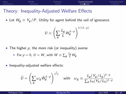
Theory: Inequality-Adjusted Welfare Effects

• Let Wg ≡ Yg/P. Utility for agent behind the veil of ignorance

U ≡(

∑g

LgLW

1−ρg

)1/(1−ρ)

• The higher ρ, the more risk (or inequality) averse

I For ρ = 0, U = W , with W ≡ ∑gLgL Wg

• Inequality-adjusted welfare effects:

U =

(∑g

ωgW1−ρg

) 11−ρ

with ωg ≡Lg (Yg/Lg )1−ρ

∑h Lh(Yh/Lh)1−ρ



Inequality-adjusted welfare effects

0 2 4 6 8 10 12 14 160

0.05

0.1

0.15

0.2

0.25

0.3

1 = 1.5 = 3

The figure plots the relationship between U, the inequality-adjusted welfare effects of the rise of China, with

U ≡(

∑g lgW1−ρg

)1/(1−ρ), and ρ which is the coefficient of relative risk aversion for the agent behind the veil of ignorance.



Initial income and changes in import competition

-3 -2 -1 0 1 2 3 4-0.025

-0.02

-0.015

-0.01

-0.005

0

0.005

0.01

0.015

0.02

0.025



Counterfactual return to autarky

• The gains from trade are 1.56% for the US, with a CV of 58%.

• Losses from trade are particularly concentrated in Central and SouthernAppalachia

• The inequality-adjusted gains from trade are higher than the standardgains from trade

Full results



Unemployment (in progress)



Matching and employment rate (Kim and Vogel 2018)

• Workers get matched to a vacancy with endogenous probability Eig

• Employers’ cost of posting a vacancy Vigs is CigPi , so their ZPC entails

ψigs =(1− νig )

CigηEig

Φig

Pi,

with labor market tightness ψigs ≡ Vigs

πigsLig.

• Since ψigs = ψig , and with a matching function Eig = AMig ψα

ig :

Eig =(AMig

) 11−α

(η(1− νig )

Cig

) α1−α(

Φig

Pi

) α1−α



Updated welfare expression

Wig =

∏∏∏s


A country ′s consumer gains

· ∏∏∏s


A group′s labor−income gains

1

1−α

• The change in the employment rate amplifies the change in real income.

• The larger α - the elasticity of the employment rate to labor markettightness - the stronger the amplification.



Amplification effect of α on the welfare changes

0 0.1 0.2 0.3 0.4 0.5 0.6 0.7-10

-5

0

5

10

15



Approximate sufficient statistic for income changes

• A Bartik-style approximation of relative income changes, for any tradeshock

ln Yg/Y ≈ 1

κ(1− α)ln ∑

s

πgs rs

I rs ≡ ∑g πgsYg/Y

I This approximate sufficient statistic is exact for κ(1− α) = 1, and almostexact in our simulations.

• In the data, we (i) test the validity of this import-competition measureand (ii) estimate α indirectly, assuming κ = 1.5.



Table: Empirical analysis of the Bartik measure as sufficient statistic

(1) (2) (3)ln yg ln yg ln yg

ln ∑s πgs rs,US 1.230∗ 1.735∗∗ 1.845∗∗

(0.727) (0.824) (0.787)

Implied α 0.458 0.614 0.637F First Stage 42.66 18.80 16.35Observations 1444 1444 1444R2 0.677 0.664 0.660

Instrument IP to other (lagged) IP to other (no lag) IP to the US

Variable yg is measured as average earnings per worker. Labor shares πgs are measured as the share of workers using the CBP data in1990 and 2000. We aggregate the shares at the 2 digit-ISIC industry level. Column (1) reports the second stage coefficient in whichimports to other HI countries and lagged employment shares are used when constructing the instrument, column (2) is analogous tocolumn (1) but does not employ lagged shares. Column (3) reports the second stage coefficient in the case in which US imports isused as an instrument (without lagged employment shares). Standard errors (in parentheses) are clustered at the state level, with *p < 0.1, ** p < 0.05, *** p < 0.001. All specifications include the same set of controls employed in our baseline κ estimation.



Conclusion

• Framework to study aggregate and distributional effects of trade

• Welfare effects are summarized in a parsimonious equation that neststhe multi-sector ACR result

• Key additional parameter κ governs strength of distributional effects

• Estimate κ combining ADH Bartik strategy with structural equationfrom model, κ ≈ 1.5

• Counterfactual analysis reveals that China shock increases averagewelfare, but some groups experience losses more than six times theaverage gain

• Adjusted for plausible measures of inequality aversion, gains in socialwelfare remain positive, and deviate only slightly from the standardaggregation.


Background

Background


Background

Equilibrium

• Excess demand for efficiency units in sector s of country i is

ELDis ≡1

wis∑j

λijsβjsYj −∑g

Eigs

• λijs , Yj and Eigs are functions of the whole matrix of wages w ≡ {wis},so system ELDis = 0 for all i , s determines all wages w

Graphically

Comparative Statics

Back


Background

Comparative Statics: Wages

• Foreign shock: Tis , τijs 6= 1 for i 6= j (x ≡ x ′/x)

• Using ELDis = 0, we can write ELD ′is = 0 as

∑g

πigsΦigπigsYig = ∑j

λijsλijsβjs ∑g

ΦjgYjg

with

Φig =

(∑k

πigk wκik

)1/κ

,

λijs =Tis (τijswis)

−θs

∑k λkjsTks (τkjswks)−θs

,

πigs =w κis

∑k πigk wκik

Back


Background

Supply and Demand of Eis

𝑫𝒆𝒎𝒂𝒏𝒅

𝑬𝒊𝒔

𝒘𝒊𝒔

𝑬𝒊𝟏𝒔

!𝑬𝒊𝒈𝒔𝒈

𝑬𝒊𝒔∗ 𝑬𝒊𝟏𝒔∗

𝒘𝒊𝒔∗

Back


Background

Derivation of estimation equation

• Labor Share: πgs =Agsw

κs

Φκg

• Hat algebra and rearranging: Φκg =

Ags wκs

πgs

• Intuition: conditional on w κs , πgs acts as a sufficient statistic for a

group’s degree of specialization

• Taking logs, noting that yg = Φg and applying to sector NM:

ln yg = ln wNM −1

κln πgNM + εgNM ,

• Focus on non-manufacturing since it is the largest sector, and onlysector with sufficiently strong first stage

Back


Background

Exclusion restriction

• Control for observables Xgt : εgt = X ′gtΘ + εgt

• Updated exclusion restriction: Turning to the second condition, oninstrument validity, note that

cov(Zgt , εgt) = ∑s∈M

∆IPChina→Otherst E [πgst−10E[εgt |πgt−10]] = 0,

• Two ways of satisfying this restriction:

I E[πgst−10E[εgt |πgt−10]

]= 0 for all s (Goldsmith-Pinkham et al. 2018)

I cov(Zgt , εgt) = ∑s∈M ∆IPChina→Otherst E [πgst−10εgt ]→ 0 (Borusyak et

al. 2018)

• This restriction relates to the ADH argument on the exogeneity of theChina shock

Back


Background

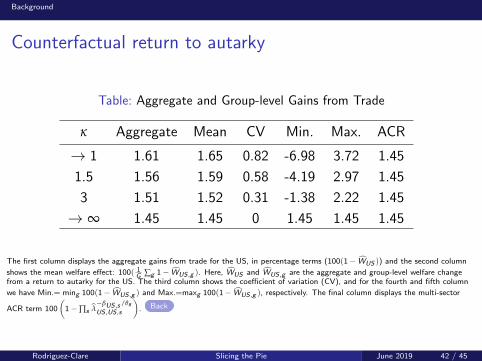
Counterfactual return to autarky

Table: Aggregate and Group-level Gains from Trade

κ Aggregate Mean CV Min. Max. ACR

→ 1 1.61 1.65 0.82 -6.98 3.72 1.45

1.5 1.56 1.59 0.58 -4.19 2.97 1.45

3 1.51 1.52 0.31 -1.38 2.22 1.45

→ ∞ 1.45 1.45 0 1.45 1.45 1.45

The first column displays the aggregate gains from trade for the US, in percentage terms (100(1− WUS )) and the second column

shows the mean welfare effect: 100( 1G ∑g 1− WUS ,g ). Here, WUS and WUS ,g are the aggregate and group-level welfare change

from a return to autarky for the US. The third column shows the coefficient of variation (CV), and for the fourth and fifth column

we have Min.= ming 100(1− WUS ,g ) and Max.=maxg 100(1− WUS ,g ), respectively. The final column displays the multi-sector

ACR term 100

(1−∏s λ

−βUS ,s /θsUS ,US ,s

). Back


Background

Figure: Geographical distribution of the gains from trade

This figure plots the geographic distribution of 100(1− Wg ), where Wg are the welfare effects for group g in the US from a return

to autarky for our preferred value of κ = 1.5. Back


Background

Inequality-adjusted Gains from Trade

0 2 4 6 8 10 12 14 160

0.5

1

1.5

2

1 = 1.5 = 3

The figure plots the relationship between the inequality-adjusted gains from trade UUS ≡(

∑g ωg W1−ρg

) 11−ρ and ρ. Here, ρ is the

coefficient of relative risk aversion for the agent behind the veil of ignorance and ωg ≡lg (Yg /Lg )

1−ρ

∑h lh(Yh/Lh)1−ρ a modified weight for group

g . The vertical axis displays 100(1− UUS ).Back


Background

Income and import competition

-3 -2 -1 0 1 2 3 4-0.04

-0.02

0

0.02

0.04

0.06

0.08

0.1

Back


lecture 2: distributional e ects of trade

Documents