Lecture 2 Announcements:

• First assignment is assigned today and due next Wed. Assignment is linked to the daily schedule on the course webpage.

• You can turn in homework Wed in class, or in slot on wall across from 2202 Bren, by 5:00pm on due date. Make sure you use the slot for the correct Lecture (A or B) for Statistics 110.

• You will need R for the homework due next week, so make sure you install R and R Studio early enough to get help if needed. See course website links under heading related to computer accounts and information.

• More information on R and R Studio in Friday discussion. Bring laptop (with R and R Studio installed) if desired.

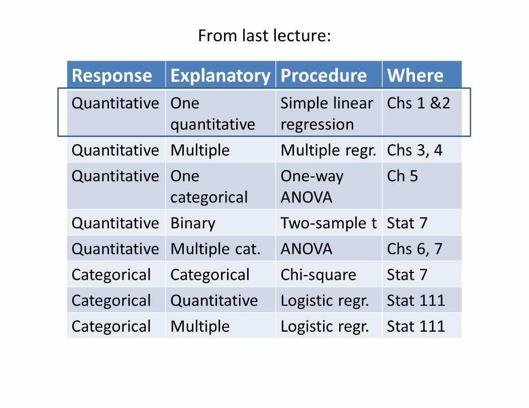
From last lecture:

TODAY:

• First half of lecture is finishing Chapter 0 (on white board) • Then Sections 1.1 and 1.2 (these notes)

Simple Linear Regression, for relationship between

Two Quantitative Variables

Motivation Measure 2 quantitative variables on the same units.

• How strongly related are they?

• In the future, if we know value of one, can we predict the other?

Example: After the midterm exam, how well can we predict your final average (of homework, midterm, final) for this class?

Data: Last year’s Stat 110 class where both midterm and final average are known. Use it to create an equation to use in the future, to predict

Y = Final Average, when X = Midterm score is known.

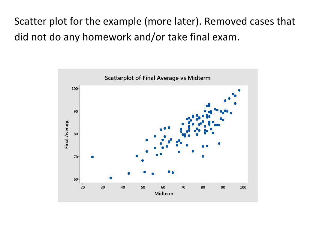
Scatter plot for the example (more later). Removed cases that did not do any homework and/or take final exam.

1009080706050403020

100

90

80

70

60

Midterm

Fina

l Ave

rage

Scatterplot of Final Average vs Midterm

Algebra Review for Linear relationship Equation for a straight line:

Y = β0 + β1X

β0 = y-intercept, the value of Y when X = 0

β1 = slope, the increase in Y when X goes up by 1 unit

Example (deterministic = exact relationship): One pint of water weighs 1.04 pounds. (“A pint’s a pound the world around.”)

Suppose a bucket weighs 3 pounds. Fill it with X pints of water. Let Y = weight of the filled bucket.

How can we find Y, when we know X? Easy!

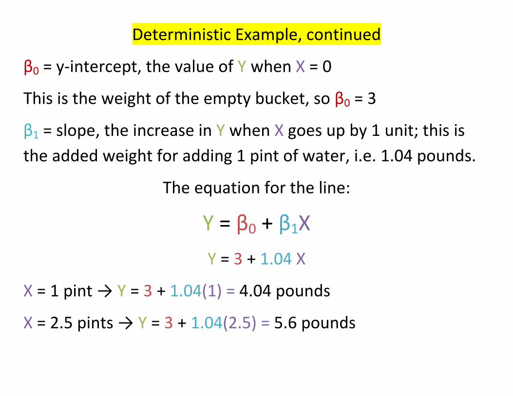
Deterministic Example, continued

β0 = y-intercept, the value of Y when X = 0

This is the weight of the empty bucket, so β0 = 3

β1 = slope, the increase in Y when X goes up by 1 unit; this is the added weight for adding 1 pint of water, i.e. 1.04 pounds.

The equation for the line:

Y = β0 + β1X Y = 3 + 1.04 X

X = 1 pint → Y = 3 + 1.04(1) = 4.04 pounds

X = 2.5 pints → Y = 3 + 1.04(2.5) = 5.6 pounds

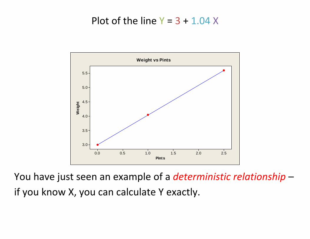
Plot of the line Y = 3 + 1.04 X

2.52.01.51.00.50.0

5.5

5.0

4.5

4.0

3.5

3.0

Pints

Wei

ght

Weight vs Pints

You have just seen an example of a deterministic relationship – if you know X, you can calculate Y exactly.

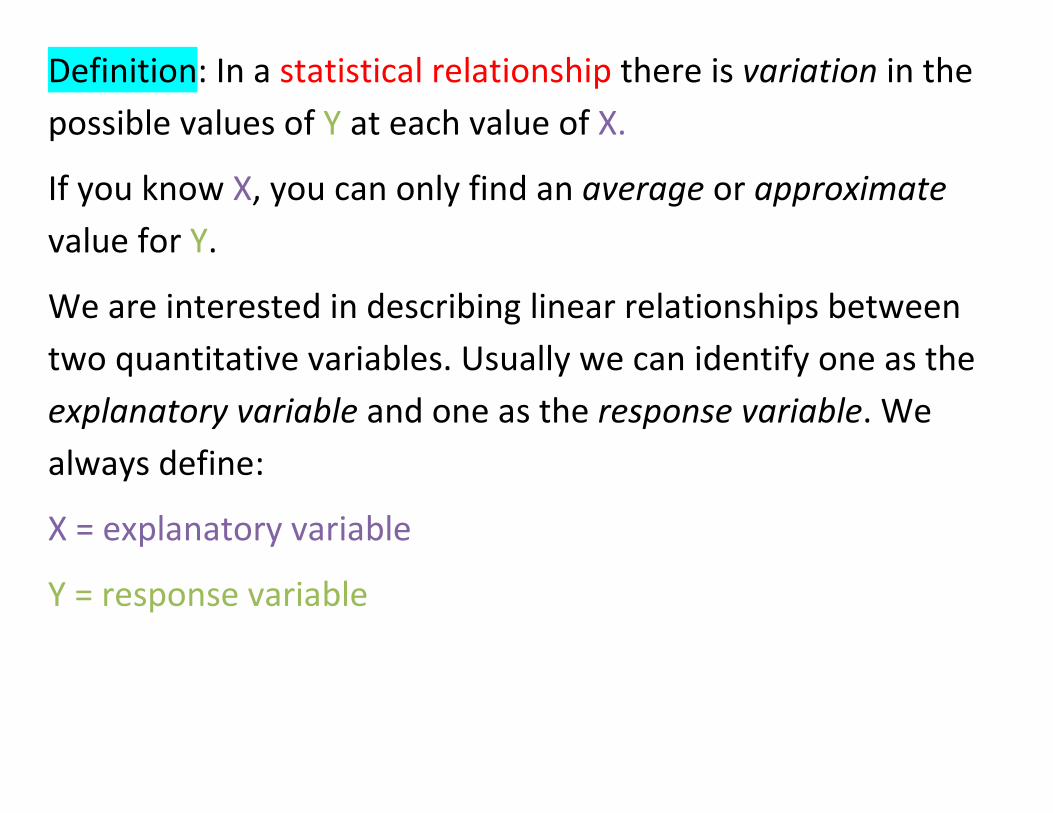
Definition: In a statistical relationship there is variation in the possible values of Y at each value of X.

If you know X, you can only find an average or approximate value for Y.

We are interested in describing linear relationships between two quantitative variables. Usually we can identify one as the explanatory variable and one as the response variable. We always define:

X = explanatory variable

Y = response variable

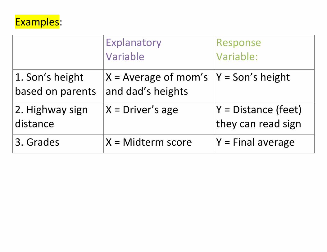
Examples:

Explanatory Variable

Response Variable:

1. Son’s height based on parents

X = Average of mom’s and dad’s heights

Y = Son’s height

2. Highway sign distance

X = Driver’s age Y = Distance (feet) they can read sign

3. Grades X = Midterm score Y = Final average

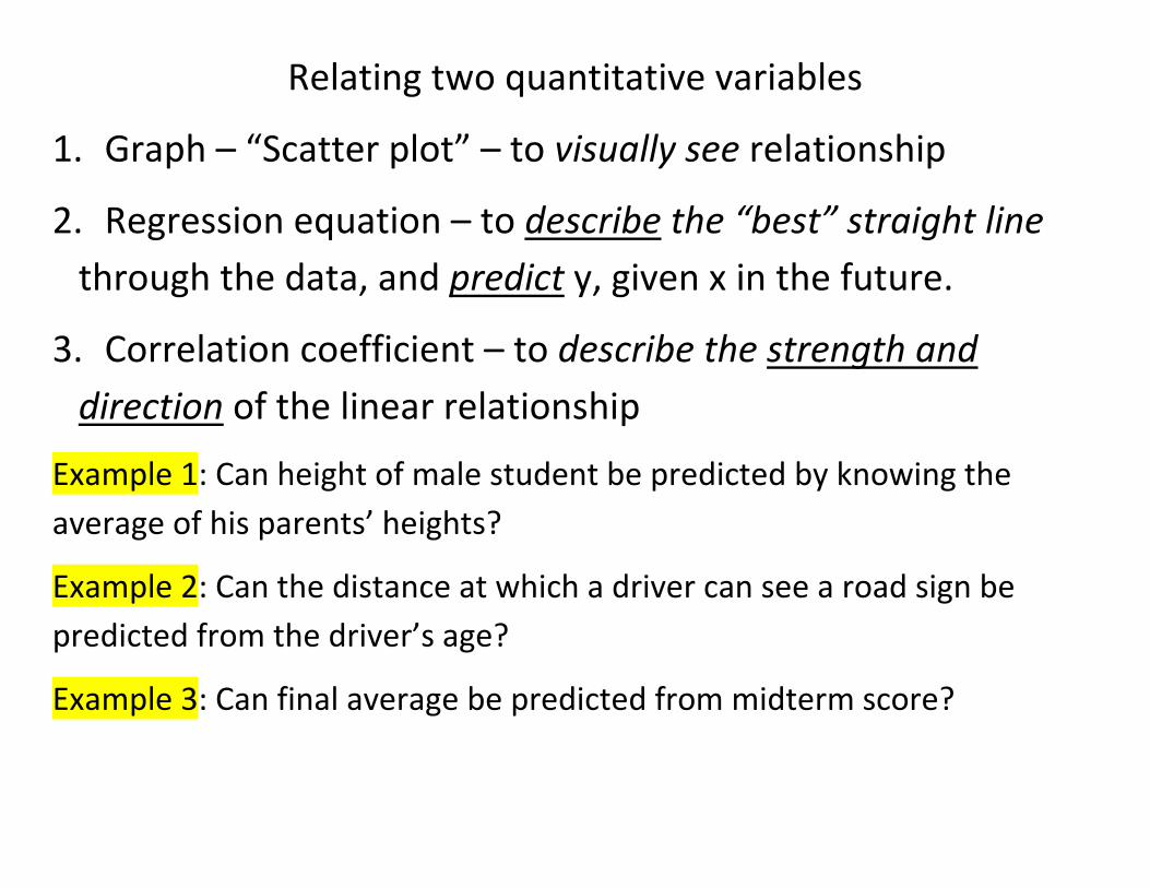
Relating two quantitative variables

1. Graph – “Scatter plot” – to visually see relationship

2. Regression equation – to describe the “best” straight line through the data, and predict y, given x in the future.

3. Correlation coefficient – to describe the strength and direction of the linear relationship

Example 1: Can height of male student be predicted by knowing the average of his parents’ heights?

Example 2: Can the distance at which a driver can see a road sign be predicted from the driver’s age?

Example 3: Can final average be predicted from midterm score?

Creating a scatter plot:

• Create axes with the appropriate ranges for X (horizontal axis) and Y (vertical axis)

• Put in one “dot” for each (x, y) pair in the data set.

Example 1: Scatterplot of 3 points, x = avg parent ht, y = height

First 3 points in the data (in inches): x y 64.5 72 68 68 69.5 70

AvgParentHt

Hei

ght

70696867666564

72

71

70

69

68

64.5 68 69.5

72

68

70

Scatterplot of Height vs AvgParentHt

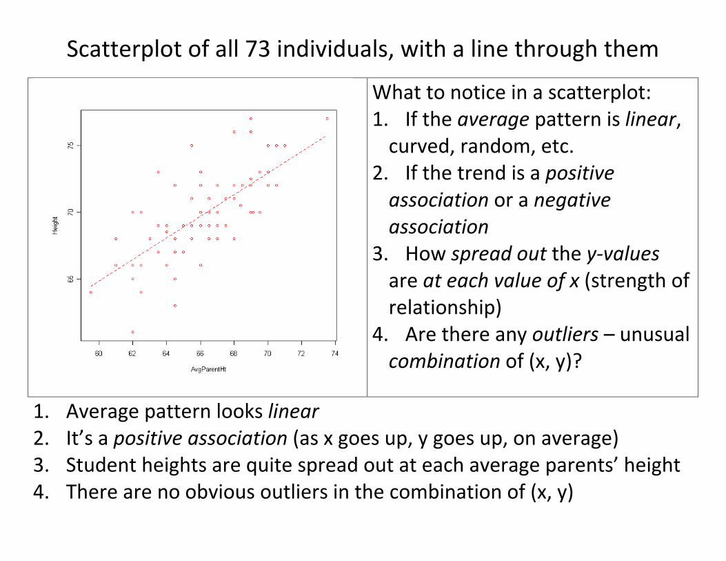
Scatterplot of all 73 individuals, with a line through them

What to notice in a scatterplot: 1. If the average pattern is linear,

curved, random, etc. 2. If the trend is a positive

association or a negative association

3. How spread out the y-values are at each value of x (strength of relationship)

4. Are there any outliers – unusual combination of (x, y)?

1. Average pattern looks linear 2. It’s a positive association (as x goes up, y goes up, on average) 3. Student heights are quite spread out at each average parents’ height 4. There are no obvious outliers in the combination of (x, y)

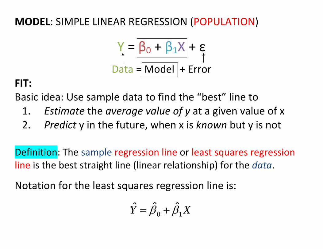
MODEL: SIMPLE LINEAR REGRESSION (POPULATION)

Y = β0 + β1X + ε Data = Model + Error

FIT: Basic idea: Use sample data to find the “best” line to

1. Estimate the average value of y at a given value of x 2. Predict y in the future, when x is known but y is not

Definition: The sample regression line or least squares regression line is the best straight line (linear relationship) for the data.

Notation for the least squares regression line is:

XY 10ˆˆˆ ββ +=

XY 10ˆˆˆ ββ +=

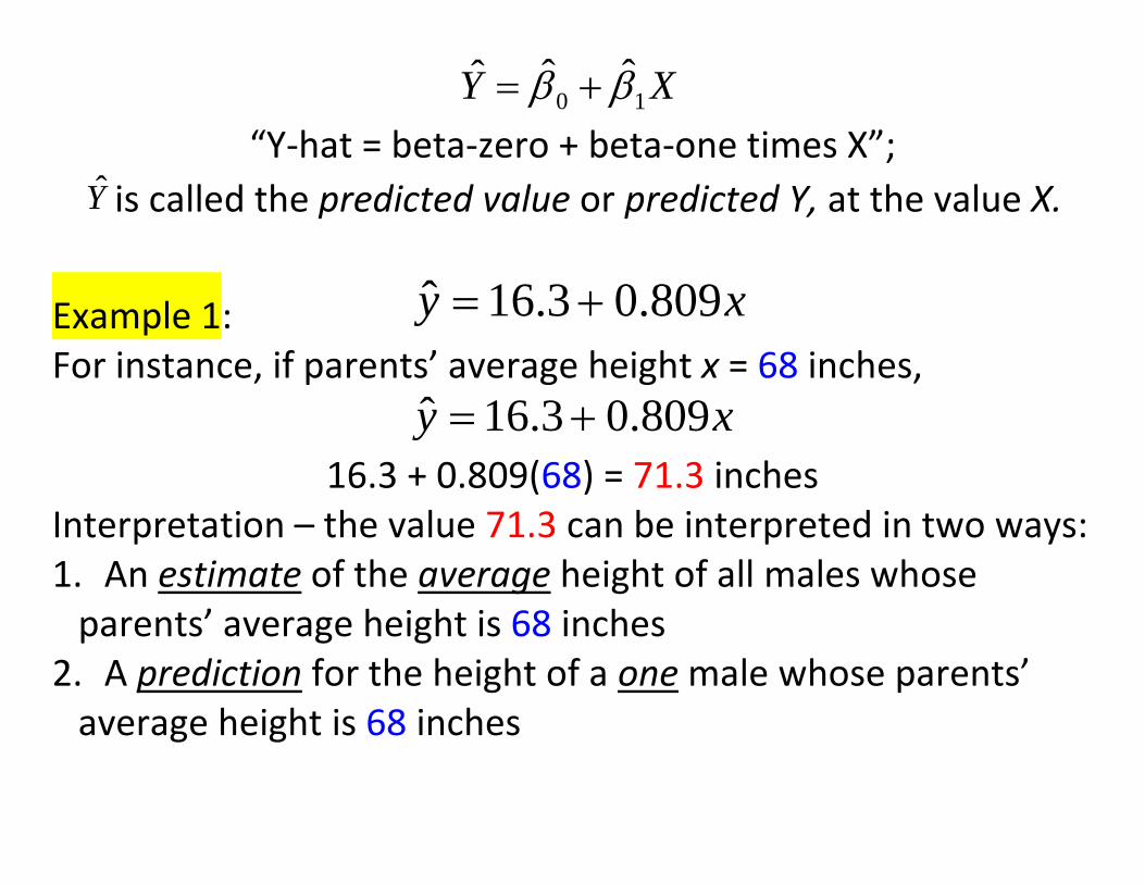
“Y-hat = beta-zero + beta-one times X”; Y is called the predicted value or predicted Y, at the value X.

Example 1: xy 809.03.16ˆ += For instance, if parents’ average height x = 68 inches,

xy 809.03.16ˆ += 16.3 + 0.809(68) = 71.3 inches

Interpretation – the value 71.3 can be interpreted in two ways: 1. An estimate of the average height of all males whose

parents’ average height is 68 inches 2. A prediction for the height of a one male whose parents’

average height is 68 inches

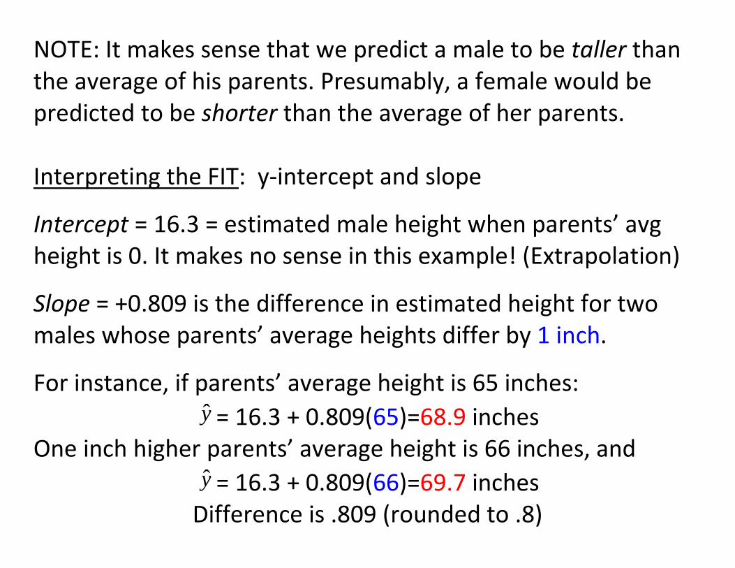
NOTE: It makes sense that we predict a male to be taller than the average of his parents. Presumably, a female would be predicted to be shorter than the average of her parents.

Interpreting the FIT: y-intercept and slope

Intercept = 16.3 = estimated male height when parents’ avg height is 0. It makes no sense in this example! (Extrapolation)

Slope = +0.809 is the difference in estimated height for two males whose parents’ average heights differ by 1 inch.

For instance, if parents’ average height is 65 inches: y = 16.3 + 0.809(65)=68.9 inches

One inch higher parents’ average height is 66 inches, and y = 16.3 + 0.809(66)=69.7 inches

Difference is .809 (rounded to .8)

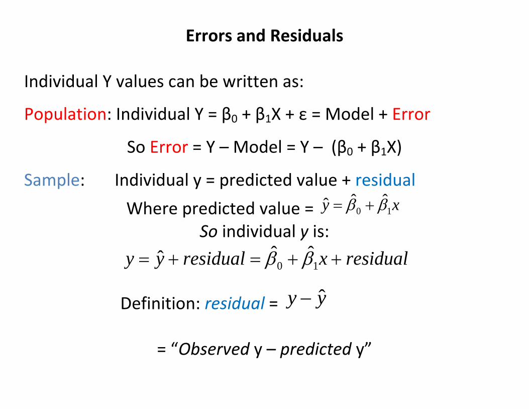
Errors and Residuals

Individual Y values can be written as:

Population: Individual Y = β0 + β1X + ε = Model + Error

So Error = Y – Model = Y – (β0 + β1X)

Sample: Individual y = predicted value + residual Where predicted value = xy 10

ˆˆˆ ββ += So individual y is:

residualxresidualyy ++=+= 10ˆˆˆ ββ

Definition: residual = ˆy y−

= “Observed y – predicted y”

Example: Suppose the average of a guy’s parents’ heights is 66 inches, and he is 69 inches tall.

Observed data: x = 66 inches, y = 69 inches.

Predicted height: y = 16.3 + 0.809(66) = 69.7 inches

Residual = 69 – 69.7 = –0.7 inches

The person is just 0.7 inches shorter than predicted.

y = predicted value + residual 69 = 69.7 + (–0.7)

Each y value in the original dataset can be written this way.

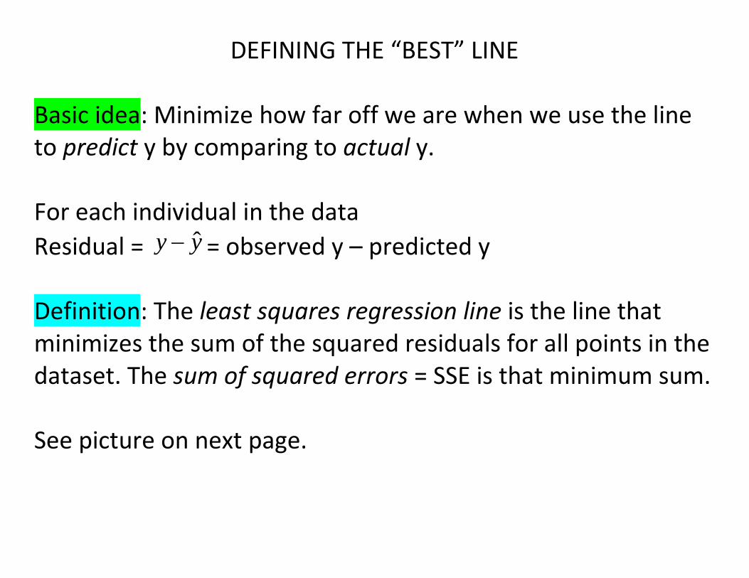
DEFINING THE “BEST” LINE Basic idea: Minimize how far off we are when we use the line to predict y by comparing to actual y. For each individual in the data Residual = yy ˆ− = observed y – predicted y Definition: The least squares regression line is the line that minimizes the sum of the squared residuals for all points in the dataset. The sum of squared errors = SSE is that minimum sum. See picture on next page.

ILLUSTRATING THE LEAST SQUARES LINE

7472706866646260

78

76

74

72

70

68

66

64

62

60

AvgParentsHt

Hei

ght

Scatterplot of Height vs Average Parents' Height

SSE = 376.9 (average of about 5.16 per person, or about 2.25 inches when take square root)

Example 1: This picture shows the residuals for 4 of the individuals. The blue line comes closer to all of the points than any other line, where “close” is defined by SSE =

∑valuesall

residual 2

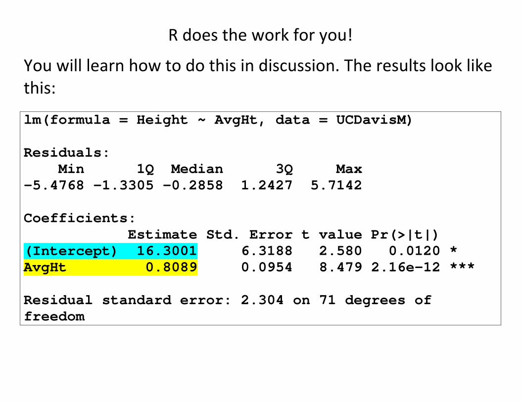
R does the work for you!

You will learn how to do this in discussion. The results look like this: lm(formula = Height ~ AvgHt, data = UCDavisM) Residuals: Min 1Q Median 3Q Max -5.4768 -1.3305 -0.2858 1.2427 5.7142 Coefficients: Estimate Std. Error t value Pr(>|t|) (Intercept) 16.3001 6.3188 2.580 0.0120 * AvgHt 0.8089 0.0954 8.479 2.16e-12 *** Residual standard error: 2.304 on 71 degrees of freedom

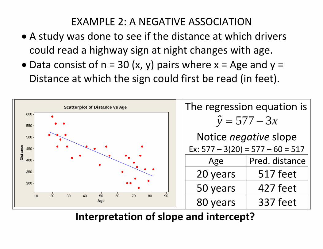
EXAMPLE 2: A NEGATIVE ASSOCIATION • A study was done to see if the distance at which drivers

could read a highway sign at night changes with age. • Data consist of n = 30 (x, y) pairs where x = Age and y =

Distance at which the sign could first be read (in feet).

Age

Dis

tanc

e

908070605040302010

600

550

500

450

400

350

300

Scatterplot of Distance vs Age

The regression equation is xy 3577ˆ −=

Notice negative slope Ex: 577 – 3(20) = 577 – 60 = 517

Age Pred. distance 20 years 517 feet 50 years 427 feet 80 years 337 feet

Interpretation of slope and intercept?

Not easy to find the best line by eye!

Applets: http://www.rossmanchance.com/applets/RegShuffle.htm (Try copying and pasting data from other examples.) http://illuminations.nctm.org/Activity.aspx?id=4187 http://illuminations.nctm.org/Activity.aspx?id=4186

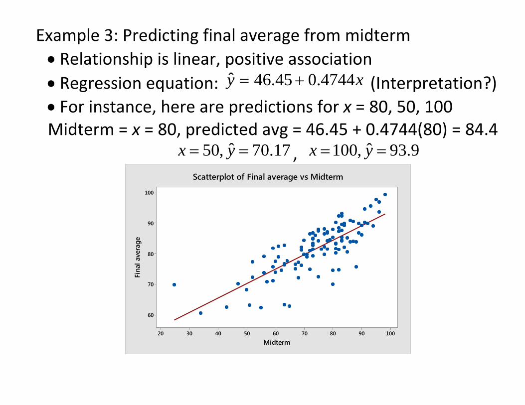
Example 3: Predicting final average from midterm • Relationship is linear, positive association • Regression equation: xy 4744.045.46ˆ += (Interpretation?) • For instance, here are predictions for x = 80, 50, 100 Midterm = x = 80, predicted avg = 46.45 + 0.4744(80) = 84.4

17.70ˆ,50 == yx , 9.93ˆ,100 == yx

1009080706050403020

100

90

80

70

60

Midterm

Fina

l ave

rage

Scatterplot of Final average vs Midterm

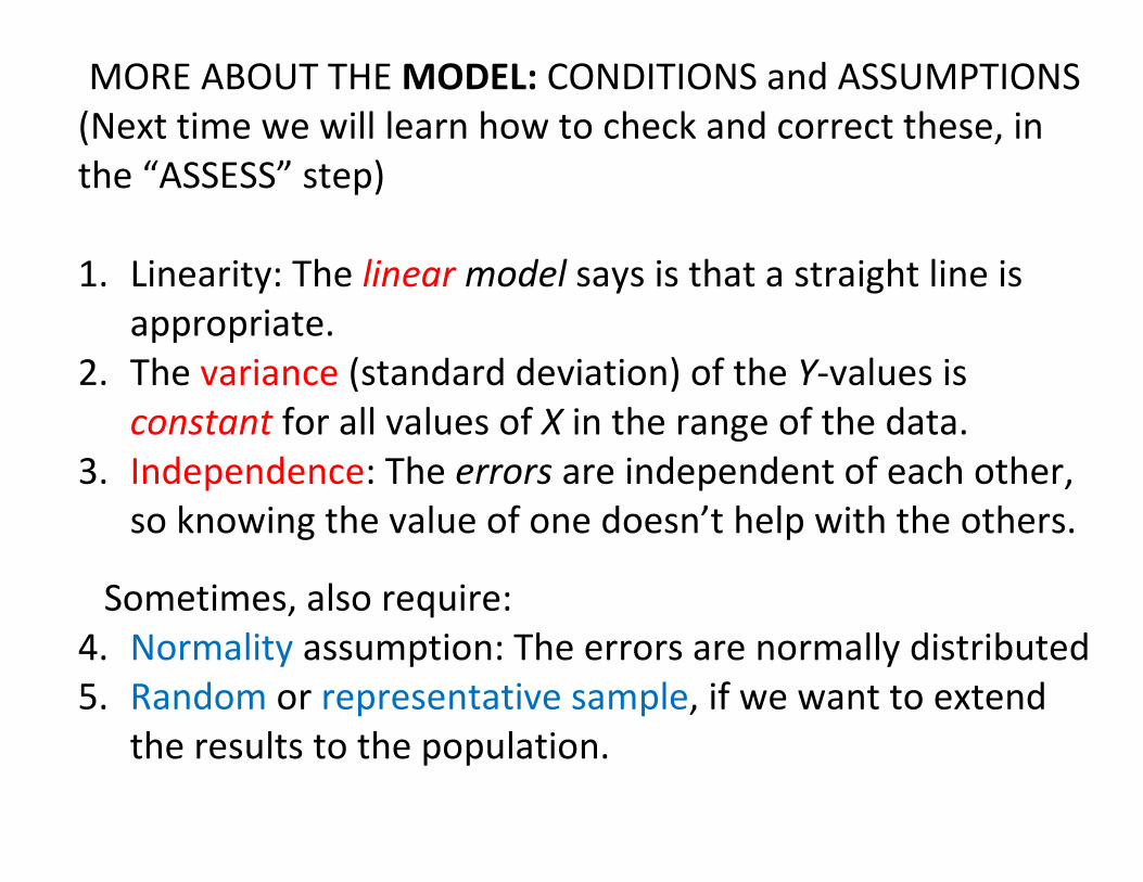
MORE ABOUT THE MODEL: CONDITIONS and ASSUMPTIONS (Next time we will learn how to check and correct these, in the “ASSESS” step)

1. Linearity: The linear model says is that a straight line is

appropriate. 2. The variance (standard deviation) of the Y-values is

constant for all values of X in the range of the data. 3. Independence: The errors are independent of each other,

so knowing the value of one doesn’t help with the others.

Sometimes, also require: 4. Normality assumption: The errors are normally distributed 5. Random or representative sample, if we want to extend

the results to the population.

Putting this all together, the Simple Linear Regression Model (for the Population) is:

Y = β0 + β1X + ε where ε ~ N(0, σ) and all independent

and σ = standard deviation errors = standard deviation of all Y values at each X value

Picture of this model:

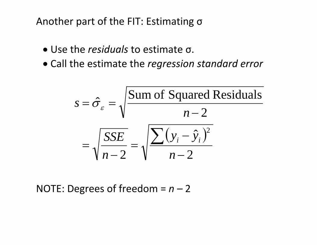
Another part of the FIT: Estimating σ • Use the residuals to estimate σ. • Call the estimate the regression standard error

( )2

ˆ2

2Residuals Squared of Sumˆ

2

−−

=−

=

−==

∑n

yynSSE

ns

ii

es

NOTE: Degrees of freedom = n – 2

Example: Highway Sign Distance

feetnSSEs 76.49

2869334

2==

−=

Interpretation: At each age, X, there is a distribution of possible distances (Y) at which sign can be read. The mean is estimated to be

xy 3577ˆ −= The standard deviation is estimated to be about 50 feet. For instance, for everyone who is 30 years old, the distribution of sign-reading distances has approximately: Mean = 577 – 90 = 487 feet and st. dev. = 50 feet. See picture on white board. For Ex 3 (grades), s = 5. Interpretation?