lecture 19 - university of california, san...

Lecture 19

• Self-organizing data structures: lists, splay trees

• Data structures for multidimensional data: K-D trees

• Review and overview of the C++ Standard Template Library

• Final review

Reading: Weiss, Ch. 4 and Ch. 12

of 31CSE 100, UCSD: LEC 19

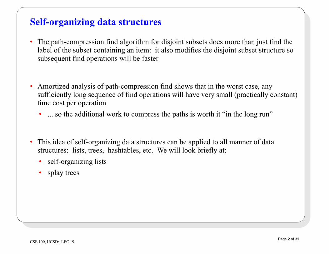
Self-organizing data structures

• The path-compression find algorithm for disjoint subsets does more than just find the label of the subset containing an item: it also modifies the disjoint subset structure so subsequent find operations will be faster

• Amortized analysis of path-compression find shows that in the worst case, any sufficiently long sequence of find operations will have very small (practically constant) time cost per operation

• ... so the additional work to compress the paths is worth it “in the long run”

• This idea of self-organizing data structures can be applied to all manner of data structures: lists, trees, hashtables, etc. We will look briefly at:

• self-organizing lists

• splay trees


Self-organizing lists

• Worst-case time cost for searching a linked list is O(N)

• Assuming all keys are equally likely to be searched for, average case time cost for successful search in a linked list is also O(N)

• But what if all keys are not equally likely?

• Then we might be able to do better by putting keys that are more likely to be searched for at the beginning of the list...


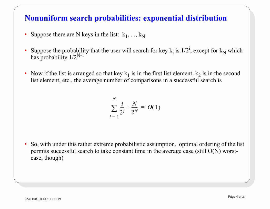
Nonuniform search probabilities: exponential distribution

• Suppose there are N keys in the list: k1, ..., kN

• Suppose the probability that the user will search for key ki is 1/2i, except for kN which has probability 1/2N-1

• Now if the list is arranged so that key k1 is in the first list element, k2 is in the second list element, etc., the average number of comparisons in a successful search is

• So, with under this rather extreme probabilistic assumption, optimal ordering of the list permits successful search to take constant time in the average case (still O(N) worst-case, though)

i2i----

i 1=

N

N2N------+ O 1 =


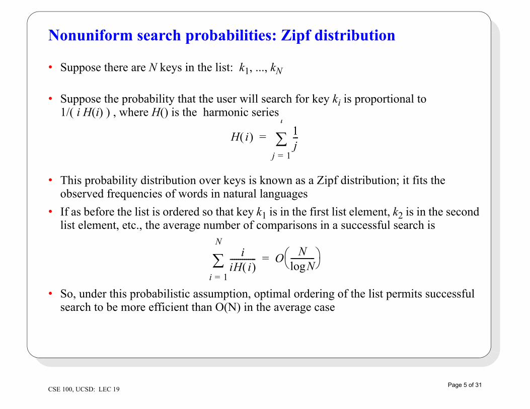
Nonuniform search probabilities: Zipf distribution

• Suppose there are N keys in the list: k1, ..., kN

• Suppose the probability that the user will search for key ki is proportional to 1/( i H(i) ) , where H() is the harmonic series

• This probability distribution over keys is known as a Zipf distribution; it fits the observed frequencies of words in natural languages

• If as before the list is ordered so that key k1 is in the first list element, k2 is in the second list element, etc., the average number of comparisons in a successful search is

• So, under this probabilistic assumption, optimal ordering of the list permits successful search to be more efficient than O(N) in the average case

H i 1j---

j 1=

i

=

iiH i -------------

i 1=

N

ONNlog

------------ =


Nonuniform search probabilities: the 90/10 rule

• The 90/10 rule: Empirical studies show that in a typical database, 90% of the references are to only 10% of the items

• (This is a rough qualitiative result that may not be true in all cases... Sometimes the same idea is called the 80/20 rule...)

• If the 90/10 rule holds, and the list is arranged so that the more frequently referenced keys are at the front of the list, average access time will be 10 times faster than in a randomly arranged list

• This is still O(N) average case, but with a better constant factor


Self-organizing list strategies

• If you know the probabilities for each key, you could build a list ordered by those probabilities (this is called the “optimal static ordering”)

• But usually you don’t know the probabilities beforehand

• A self-organizing list will adapt to the actual pattern of searches, by moving a found key nearer to the front of the list (insert and delete operations can stay the same)

• There are two simple strategies for this: transpose and move-to-front


Transpose

• When there is a successful search for a key in the list, swap that key with the key in the previous element in the list

• Easy to do, whether the list is implemented as a pointer-based linked list or as an array

• Eventually, frequently accessed keys will tend to move near the front of the list...

• ... but they are not guaranteed to do so!

• Consider this “worst case” situation: The list is created, and then only the last two elements are accessed alternately

• these two elements will repeatedly be exchanged with each other, and will stay at the end of the list


Move-to-front

• When there is a successful search for a key in the list, move the element with that key to the front of the list

• Easy to do in a pointer-based linked list, more expensive in a list implemented with an array

• Obviously, over time, frequently accessed keys will tend to be near the front of the list

• In fact, it can be shown that the average number of comparisons for a successful search using the simple move-to-front strategy is no more than twice that of the optimal static ordering!


Self-organizing search trees

• The ideas of self-organizing lists can be applied to search trees as well

• Basic idea: when a search operation finds a key in the tree, move the node containing that key to the root of the tree, so subsequent accesses will be fast

• This can be done using repeated AVL single rotations, rotating the node up to the root

• This idea was originally proposed by Allen and Munro [1978] and by Bitner [1979]

• However, simply rotating the node with a found key to the root has worst-case amortized cost O(N) per operation (because the tree can become, and remain, very unbalanced)

• Something better is needed...


Splay trees

• Splay trees were proposed by Sleator and Tarjan [1985]

• Splay trees are binary search trees that use “splaying” operations after a successful find to move the found key to the root of the tree. These operations improve subsequent searches for that key, while not making access for other keys worse on average

• Splaying operations are composed out of AVL rotations involving a node, its parent, and grandparent, depending on various special cases.

• The result: worst-case amortized time cost for any sequence of M > N find operations is O(M log N) , so splay trees act like balanced trees “in the long run”

• (However, worst-case time cost for any individual find operation is still O(N) )


Search trees and multidimensional keys

• The search trees we have discussed so far (ordinary binary search trees, AVL trees, red-black trees, B trees, treaps, splay trees) require that the set of possible keys be completely ordered

• for each pair of keys K1, K2 exactly one of these is true:

• K1 < K2

• K1 = K2

• K1 > K2

• That means that the possible keys must lie in a one-dimensional set (or anyway be mapped to a one-dimensional set by the ordering relation)

• What to do if the keys are multidimensional?


Multidimensional keys

• Example 1: In a database of persons, the key may be a pair of strings (lastname, firstname)

• Example 2: In a database of 3D graphics objects, the key may be an ordered triple of numbers (x,y,z) which are the Cartesian x,y,z coordinates of the center of the object

• How can these keys be stored in a search tree?


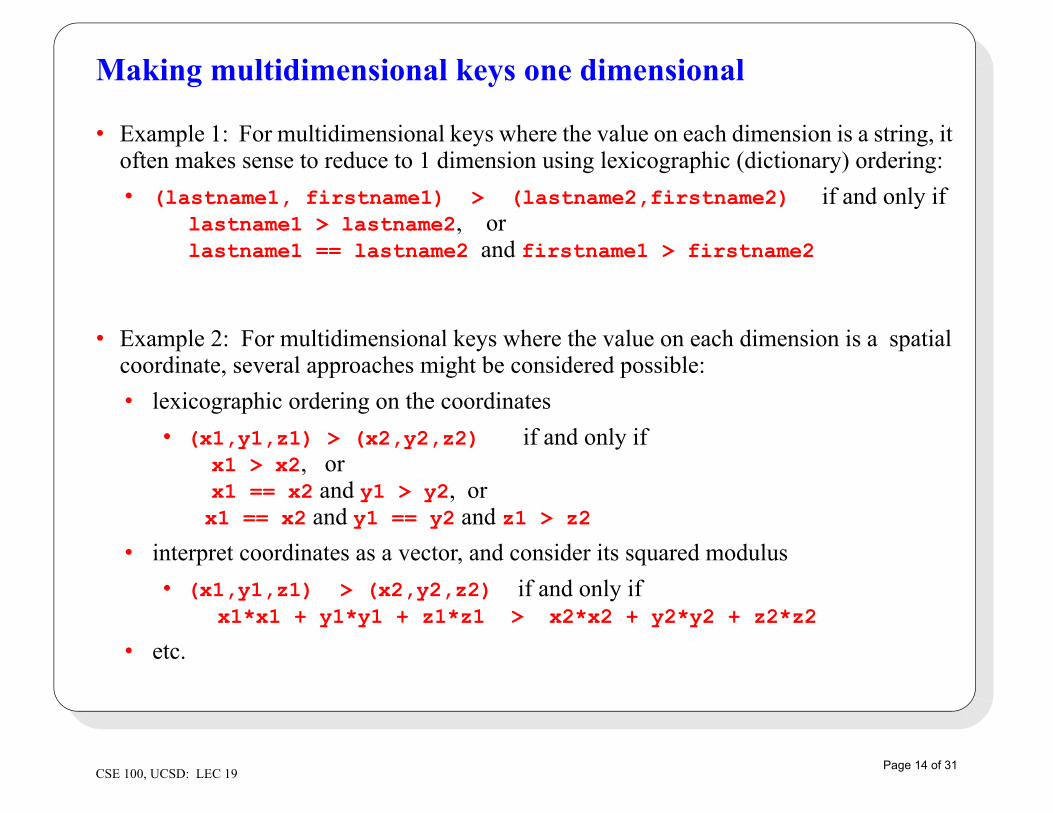
Making multidimensional keys one dimensional

• Example 1: For multidimensional keys where the value on each dimension is a string, it often makes sense to reduce to 1 dimension using lexicographic (dictionary) ordering:

• (lastname1, firstname1) > (lastname2,firstname2) if and only if lastname1 > lastname2, or lastname1 == lastname2 and firstname1 > firstname2

• Example 2: For multidimensional keys where the value on each dimension is a spatial coordinate, several approaches might be considered possible:

• lexicographic ordering on the coordinates

• (x1,y1,z1) > (x2,y2,z2) if and only if x1 > x2, or x1 == x2 and y1 > y2, or x1 == x2 and y1 == y2 and z1 > z2

• interpret coordinates as a vector, and consider its squared modulus

• (x1,y1,z1) > (x2,y2,z2) if and only if x1*x1 + y1*y1 + z1*z1 > x2*x2 + y2*y2 + z2*z2

• etc.


Keeping multidimensional keys multidimensional

• As you know, search trees require ordered keys

• One advantage of search trees (over hashtables) is that the key ordering information can be used to make some interesting queries efficient. For example:

• find the 10 names in the database that are alphabetically nearest the given name, or

• find the 7 objects in the database whose centers are geometrically nearest the given object, etc.

• But if you map multidimensions to 1D, you may lose the ordering information you need for such queries

• This is particularly a problem in spatial or geometric applications: nearness of coordinates is not preserved with lexicographic ordering or comparing vector moduli

• The solution is to use a search tree that deals directly with multidimensional keys


K-D trees

• k-d trees are a variation on the BST that allows for efficient processing of multidimensional keys (k-d is an abbreviation of “k-dimensional”)

• k-d trees differ from BST’s in that each level of the k-d tree makes branching decisions based on one of the k dimensions of the key

• If a key has k dimensions 0 ,..., k-1, then tree nodes at level L make branching decisions based on key dimension L mod k

• For example, in a 3-d tree with keys (x,y,z), the root makes branching decisions on the value of the x coordinate; children of the root discriminate on the y coordinate; grandchildren of the root discriminate on z; children of the grandchildren of the root discriminate on x, etc.

• This branching decisions are just like those in a BST

• the only difference is that they “pay attention” to only one dimension of the key, and which dimension depends on the level of the node

• (of course equality comparisons need to pay attention to all dimensions of the key)


K-D tree ordering property

• k-d tree ordering property:

• Consider any node X at level L; suppose it contains a key whose dimension L mod k has value V.

• Then all keys in the left subtree of X have keys whose dimension L mod k has value less than V, and

• all keys in the right subtree of X have keys whose dimension L mod k has value greater than or equal to V


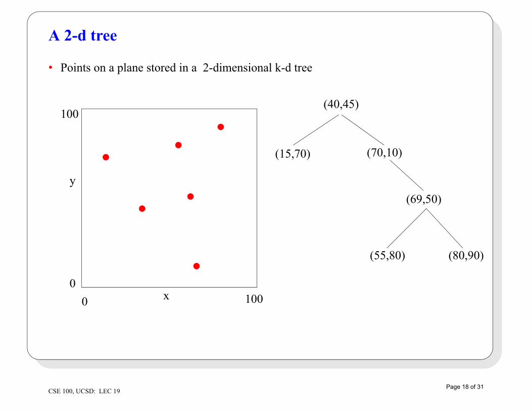
A 2-d tree

• Points on a plane stored in a 2-dimensional k-d tree

x

y

0

0

100

100

(40,45)

(15,70) (70,10)

(69,50)

(80,90)(55,80)


K-D tree operations

• Find and insert operations in k-d trees are similar to standard BST operations

• Descend the tree, making decisions at each node

• But in a k-d tree, these decisions depend on the level of the node!

• The result of an insert operation is a new leaf node

• Non-lazy delete operations are a little harder: finding the node to actually remove from the tree requires some thought

• k-d trees have the same asymptotic time costs as ordinary BST’s

• (balanced k-d trees are very tricky to implement)

• k-d trees can also be used to perform “region” queries


K-D tree region queries

• Suppose you want to find all the points that lie in a k-dimensional “hypercube” region of a certain size, centered on a certain point

• This is pretty easy to do in a k-d tree:

• Start at the root. If it is in the region, add it to the list, and recursively process its left and right children.

• If any node encountered in the search is not in the region, then check to see if it is because of the coordinate that this node is “paying attention” to

• If so, then the entire left or right subtree (depending on the result of the comparison) of this node can be eliminated from the search

• Example: Find all keys that lie within a certain hypercube


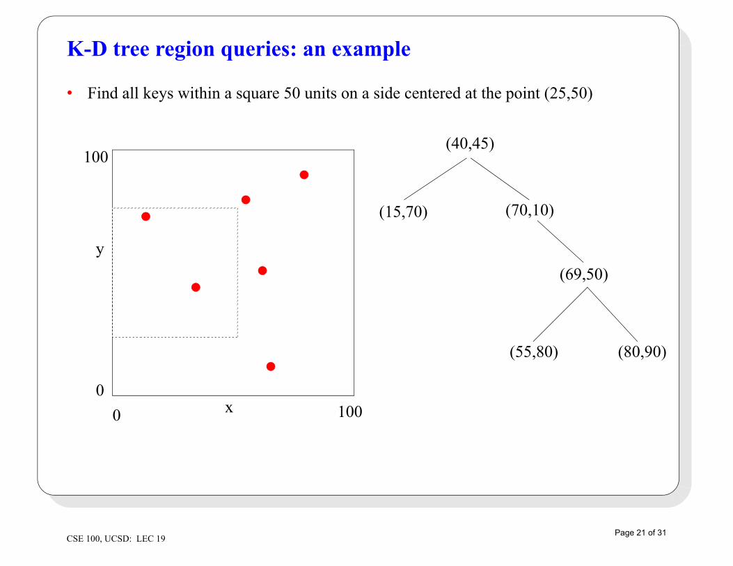
K-D tree region queries: an example

• Find all keys within a square 50 units on a side centered at the point (25,50)

x

y

0

0

100

100

(40,45)

(15,70) (70,10)

(69,50)

(80,90)(55,80)


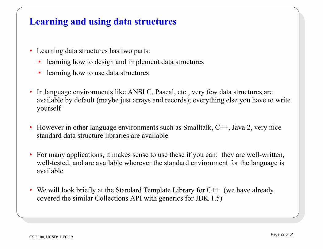
Learning and using data structures

• Learning data structures has two parts:

• learning how to design and implement data structures

• learning how to use data structures

• In language environments like ANSI C, Pascal, etc., very few data structures are available by default (maybe just arrays and records); everything else you have to write yourself

• However in other language environments such as Smalltalk, C++, Java 2, very nice standard data structure libraries are available

• For many applications, it makes sense to use these if you can: they are well-written, well-tested, and are available wherever the standard environment for the language is available

• We will look briefly at the Standard Template Library for C++ (we have already covered the similar Collections API with generics for JDK 1.5)


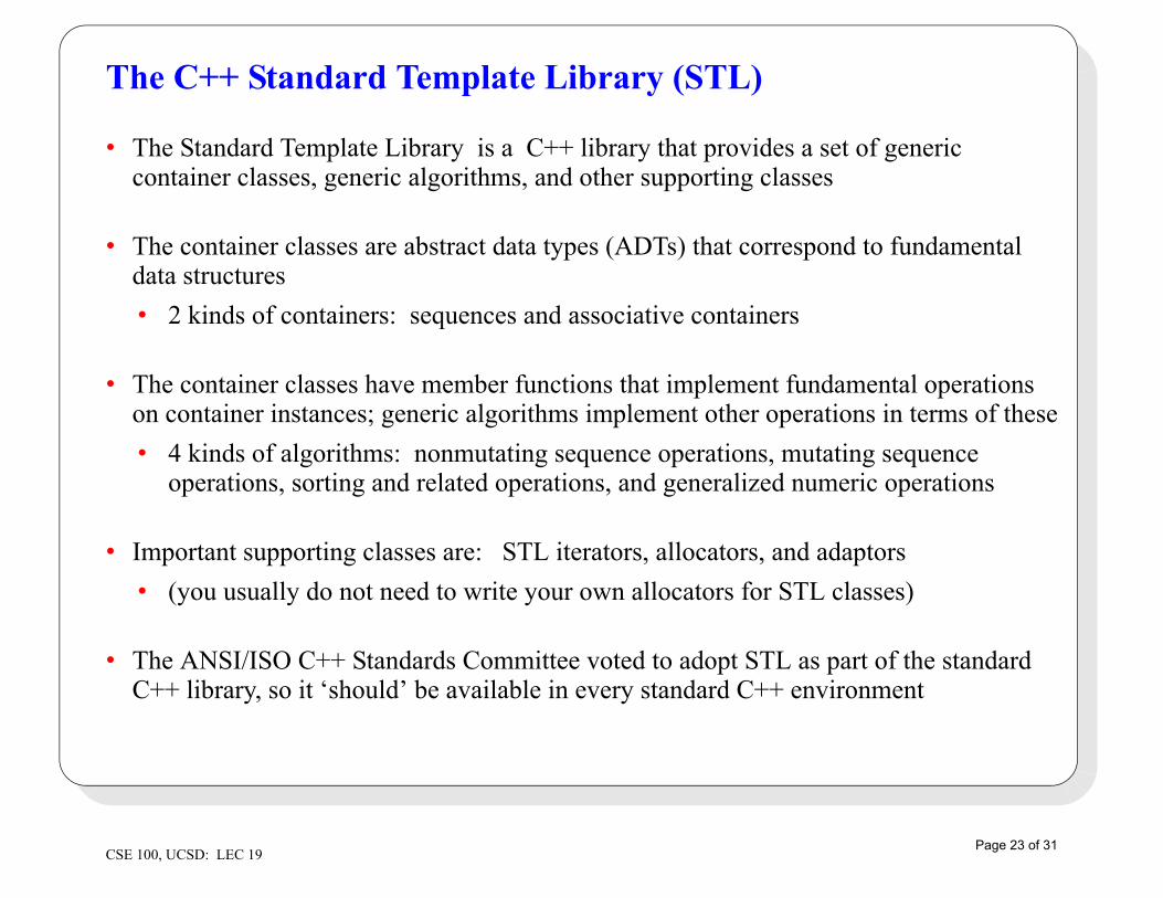
The C++ Standard Template Library (STL)

• The Standard Template Library is a C++ library that provides a set of generic container classes, generic algorithms, and other supporting classes

• The container classes are abstract data types (ADTs) that correspond to fundamental data structures

• 2 kinds of containers: sequences and associative containers

• The container classes have member functions that implement fundamental operations on container instances; generic algorithms implement other operations in terms of these

• 4 kinds of algorithms: nonmutating sequence operations, mutating sequence operations, sorting and related operations, and generalized numeric operations

• Important supporting classes are: STL iterators, allocators, and adaptors

• (you usually do not need to write your own allocators for STL classes)

• The ANSI/ISO C++ Standards Committee voted to adopt STL as part of the standard C++ library, so it ‘should’ be available in every standard C++ environment


STL iterators

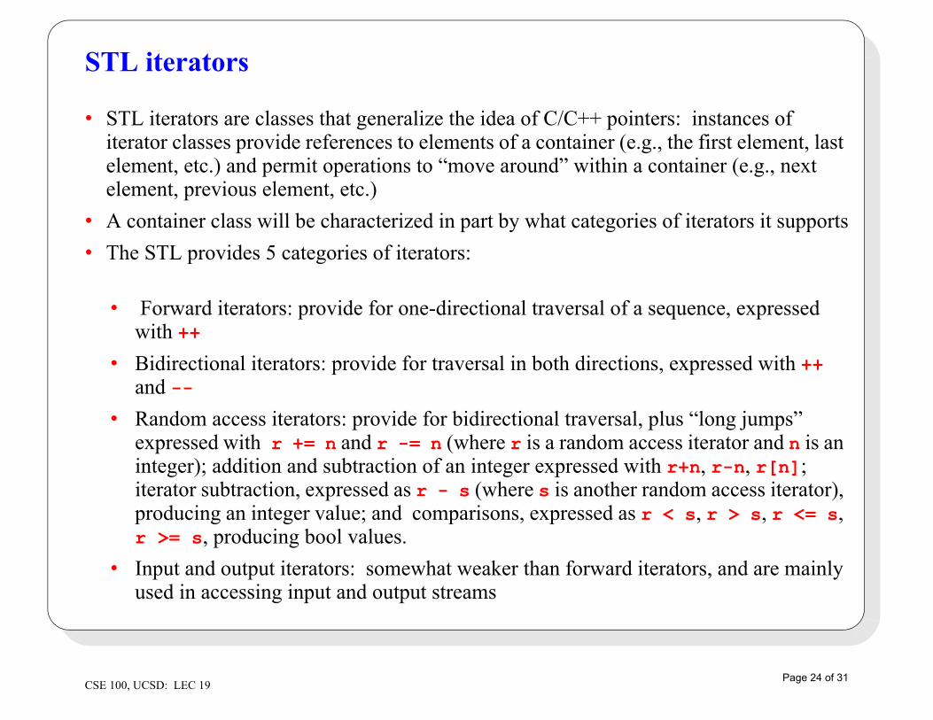
• STL iterators are classes that generalize the idea of C/C++ pointers: instances of iterator classes provide references to elements of a container (e.g., the first element, last element, etc.) and permit operations to “move around” within a container (e.g., next element, previous element, etc.)

• A container class will be characterized in part by what categories of iterators it supports

• The STL provides 5 categories of iterators:

• Forward iterators: provide for one-directional traversal of a sequence, expressed with ++

• Bidirectional iterators: provide for traversal in both directions, expressed with ++ and --

• Random access iterators: provide for bidirectional traversal, plus “long jumps” expressed with r += n and r -= n (where r is a random access iterator and n is an integer); addition and subtraction of an integer expressed with r+n, r-n, r[n]; iterator subtraction, expressed as r - s (where s is another random access iterator), producing an integer value; and comparisons, expressed as r < s, r > s, r <= s, r >= s, producing bool values.

• Input and output iterators: somewhat weaker than forward iterators, and are mainly used in accessing input and output streams


STL containers: sequences

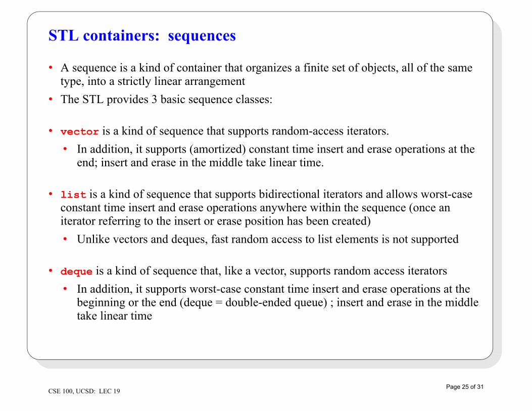
• A sequence is a kind of container that organizes a finite set of objects, all of the same type, into a strictly linear arrangement

• The STL provides 3 basic sequence classes:

• vector is a kind of sequence that supports random-access iterators.

• In addition, it supports (amortized) constant time insert and erase operations at the end; insert and erase in the middle take linear time.

• list is a kind of sequence that supports bidirectional iterators and allows worst-case constant time insert and erase operations anywhere within the sequence (once an iterator referring to the insert or erase position has been created)

• Unlike vectors and deques, fast random access to list elements is not supported

• deque is a kind of sequence that, like a vector, supports random access iterators

• In addition, it supports worst-case constant time insert and erase operations at the beginning or the end (deque = double-ended queue) ; insert and erase in the middle take linear time


STL containers: associative containers

• Associative containers provide an ability for fast retrieval of data based on keys

• The STL provides 4 basic kinds of associative containers: set, multiset, map, multimap

• All of the associative containers are parameterized (templatized) on the key type, and on an ordering relation that imposes a total order on keys

• map and multimap are also parameterized on the type of the associated data

• set and map support only unique keys; multiset and multimap allow multiple occurrences of the same key

• All associative containers support bidirectional iterators

• All associative containers support worst-case logarithmic-time insert, erase, and find operations

• Iterators for associative containers iterate through the containers in ascending order of key values


Implementing STL containers

• The STL containers have an interface that specifies required operations, and worst-case or amortized time cost bounds on the operations

• What would you use to implement the STL list class? The STL map class?

• In SGI’s reference implementation of the STL, list is implemented using doubly-linked lists, and map is implemented using red-black trees


STL algorithms

• In the STL, some algorithms are provided that are separate from any container class; this permits using the algorithms on user-defined classes and primitive types

• There are 4 kinds of these algorithms: nonmutating sequence operations, mutating sequence operations, sorting and related operations, and generalized numeric operations

• Nonmutating sequence algorithms: foreach, find, adjacent find, count, mismatch, equal, search

• Mutating sequence algorithms: copy, swap, transform, replace, fill, generate, remove, unique, reverse, rotate, random shuffle, partition

• Sorting and related algorithms: sort, nth-element, binary search, merge, set includes, set union, set intersection, set difference, set symmetric difference, minimum, maximum, lexicographic comparison, permutation generation

• Generalized numeric algorithms: accumulate, inner product, partial sum, adjacent difference


STL adaptors

• Adaptors are templated classes that “convert” a container class into one that has a different, more restrictive interface

• stack: Any sequence that supports operations back, push_back, pop_back can be used to instantiate stack. In particular, vector, list and deque can be used

• queue: Any sequence that supports operations front, back, push_back, pop_front can be used to instantiate queue. In particular, list and deque can be used

• priority queue: Any sequence with random access iterator and supporting operations front, push_back and pop_back can be used to instantiate priority_queue. In particular, vector and deque can be used


Final review

• ... any questions?!!?


Topics for the course, day 1... How did we do?

• In CSE 100, we will build on what you have already learned about programming: procedural and data abstraction, object-oriented programming, and elementary data structure and algorithm design, implementation, and analysis

• We will build on that, and go beyond it, to learn about more advanced, high-performance data structures and algorithms:

• Balanced search trees: AVL, red-black, B-trees

• Binary tries and Huffman codes for compression

• Graphs as data structures, and graph algorithms

• Data structures for disjoint-subset and union-find algorithms

• More about hash functions and hashing techniques

• Randomized data structures: skip lists, treaps

• Structures and algorithms for document database indexing

• Amortized cost analysis

• The C++ standard template library (STL)


lecture 19 - university of california, san...

Documents