lecture 17

NASSP Masters 5003F - Computational Astronomy - 2009

Lecture 17

• Reprise: dirty beam, dirty image.

• Sensitivity

• Wide-band imaging

• Weighting– Uniform vs Natural– Tapering– De Villiers weighting– Briggs-like schemes


Reprise: dirty beam, dirty image.• Fourier inversion of V times the sampling

function S gives the dirty image ID:

• This is related to the ‘true’ sky image I´ by:

• The dirty beam B is the FT of the sampling function:

• (Can get B by setting all the V to 1, then FT.)

vmulivuSvuVdvdumlI 2D e,,,

mlBmlImlI ,,,D

vmulivuSdvdumlB 2e,,


Reprise: l and m• Remember that l = sin θ. θ is the angle from

the phase centre.

• For small l, l ~ θ (in radians of course).• m is similar but for the orthogonal direction.

Direction of phase centre.

Direction ofsource.

l

θ


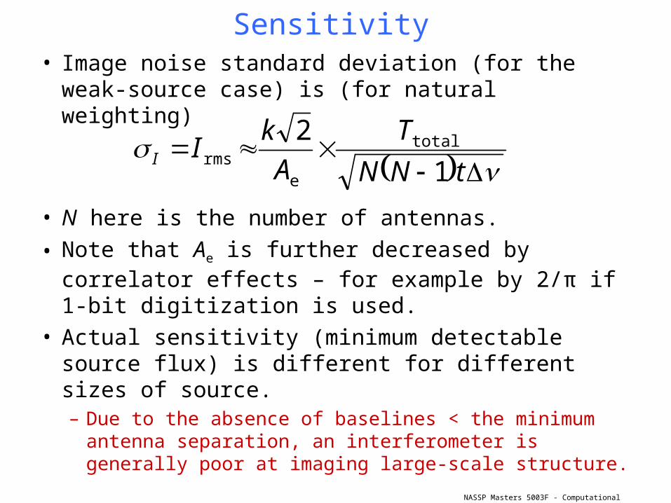
Sensitivity• Image noise standard deviation (for the weak-

source case) is (for natural weighting)

• N here is the number of antennas.

• Note that Ae is further decreased by correlator effects – for example by 2/π if 1-bit digitization is used.

• Actual sensitivity (minimum detectable source flux) is different for different sizes of source.– Due to the absence of baselines < the minimum

antenna separation, an interferometer is generally poor at imaging large-scale structure.

tNN

T

A

kII

1

2 total

erms


How can we increase UV coverage?…we could get more baselines if we moved the antennas!

Wide-band imaging.


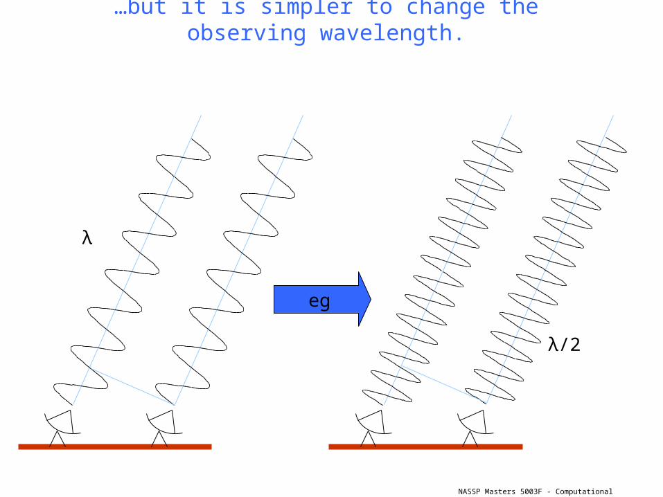
…but it is simpler to change the observing wavelength.

eg

λ

λ/2


…we have many baselines,

and, effectively,

many antennas.

With many wavelengths…

Talk at Nagoya University IMS Oct 2009

A simulated example.The full visibility function V(u,v)

(real part only shown). A familiar pattern of ‘sources’

Red positive; blue negative.

(I’ve taken some liberties here – obviously the stars of the Southern Cross arenot strong radio sources – I’ve also rescaled their angular separations.)

21/43


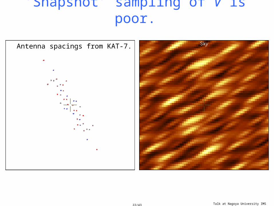
‘Snapshot’ sampling of V is poor.

Antenna spacings from KAT-7.

22/43


Aperture synthesis via the Earth’s rotation.

Dirty image D is the true sky brightness map I, convolved with the dirty beam B.


For this technique to work perfectly, all sources must be constant over time.

23/43


Frequency synthesis.


Bandwidth 5 to 6 GHz.

For this technique to work perfectly, all sources must not only be constant over time, but must also have the same spectra.

The final image is still not as ‘clean’ as we would like…

24/43


16 x 1 MHz 2000 x 1 MHz

Merlin, δ=+35° eMerlin, δ=+35°

Narrow vs broad-band: UV coverage


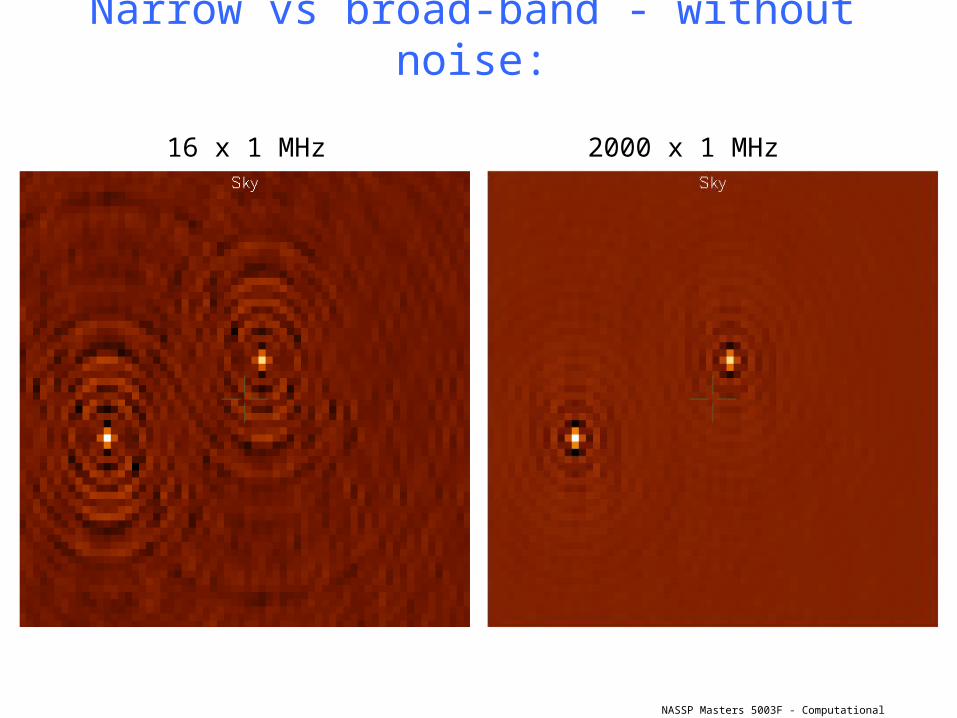
16 x 1 MHz 2000 x 1 MHz

Narrow vs broad-band - without noise:


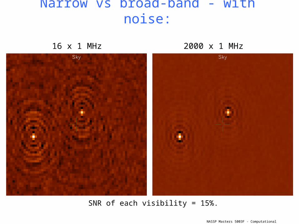
SNR of each visibility = 15%.

16 x 1 MHz 2000 x 1 MHz

Narrow vs broad-band - with noise:


Weighting: or how to shape the dirty beam.

• Why should we weight the visibilities before transforming to the sky plane?– Because the uneven distribution of samples of V means that the dirty beam has lots of ripples or sidelobes, which can extend a long way out.

• These can hide fainter sources.

– Even if we can subtract the brighter sources, there are always errors in our knowledge of the dirty beam shape.

• If there must be some residual, the smoother and lower it is, the better.


Weighting

• There are usually far more short than long baselines.

Baseline length

The distribution of baselinesalso nearly always hasa ‘hole’ in the middle.


Weighting• A crude example:

This bin has 1 sample.

This bin has 84 samples.


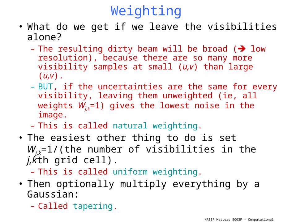
Weighting• What do we get if we leave the visibilities alone?

– The resulting dirty beam will be broad ( low resolution), because there are so many more visibility samples at small (u,v) than large (u,v).

– BUT, if the uncertainties are the same for every visibility, leaving them unweighted (ie, all weights Wj,k=1) gives the lowest noise in the image.

– This is called natural weighting.

• The easiest other thing to do is set Wj,k=1/(the number of visibilities in the j,kth grid cell).– This is called uniform weighting.

• Then optionally multiply everything by a Gaussian:– Called tapering.


Natural weighting Uniform weighting

Natural vs uniform:



The resulting dirty images:


SNR of each visibility = 0.7%.


But if we add in some noise...


Tradeoff

• This sort of tradeoff, between increasing resolution on the one hand and sensitivity on the other, is unfortunately typical in interferometry.


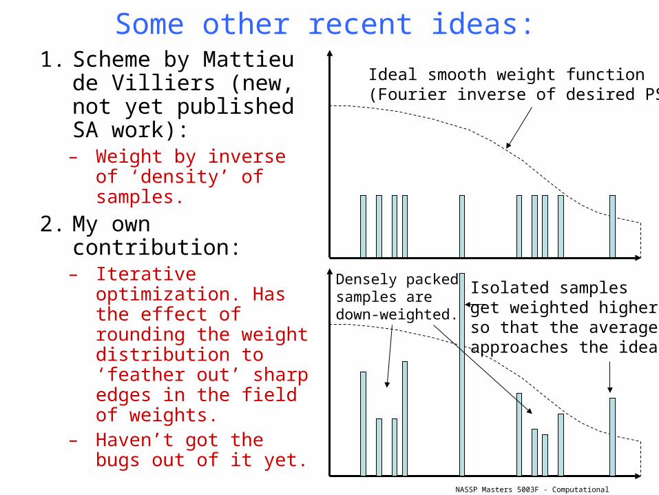
Some other recent ideas:1. Scheme by Mattieu

de Villiers (new, not yet published SA work):– Weight by inverse of

‘density’ of samples.

2. My own contribution:– Iterative optimization.

Has the effect of rounding the weight distribution to ‘feather out’ sharp edges in the field of weights.

– Haven’t got the bugs out of it yet.

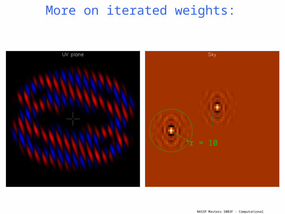
Ideal smooth weight function(Fourier inverse of desired PSF)

Isolated samplesget weighted higherso that the averageapproaches the ideal.

Densely packedsamples aredown-weighted.


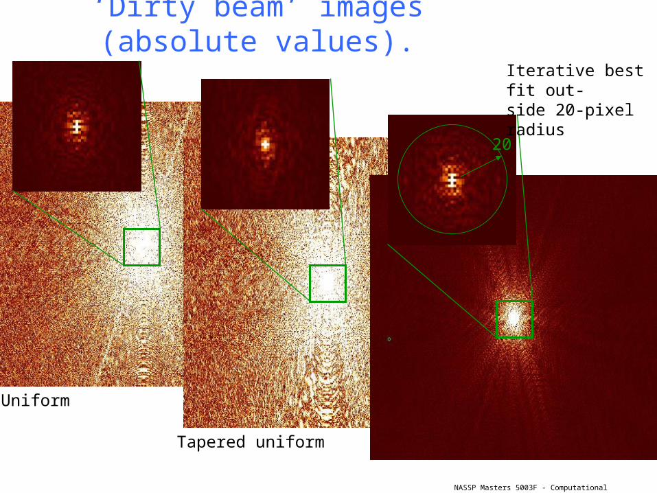
Uniform

Tapered uniform

Iterative best fit out-side 20-pixel radius

Simulated e-Merlin data.400 x 5 MHz channels;νav = 6 GHz;tint = 10 s;δ = +30°

Weighting schemes:


‘Dirty beam’ images (absolute values).

20

Iterative best fit out-side 20-pixel radius

Tapered uniform

Uniform


Natural

Uniform

Optimized

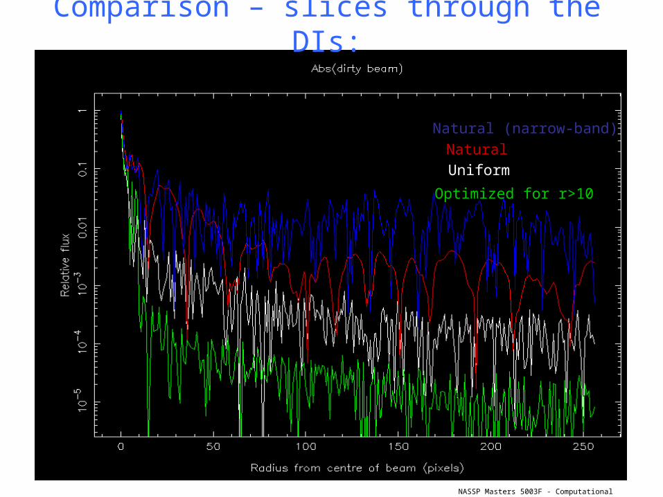
Natural (narrow-band)

Natural

Uniform

Optimized for r>10

Comparison – slices through the DIs:


r = 10

More on iterated weights:


SNR of each visibility = 5.

But real data is noisy…


1. Multiply visibilitieswith a vignettingfunction of time andfrequency, eg

2. Aips task IMAGRparameter UVBOX:effectively smoothsthe weight function.See also D Briggs’PhD thesis.

One could think of other ‘feathering’ schemes.

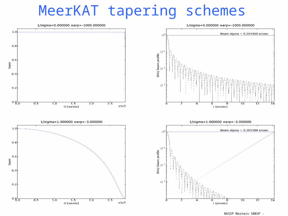
MeerKAT tapering schemes


lecture 17

Documents