lecture 16 -analysis of alternatives - us epa › sites › production › files › 2015-07 ›...

LECTURE #16

ANALYSIS OF ALTERNATIVES:MODELING SCENARIOS, BMPS, AND TMDLS

2 of 56

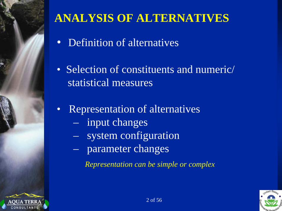
ANALYSIS OF ALTERNATIVES

• Definition of alternatives

• Selection of constituents and numeric/statistical measures

• Representation of alternatives – input changes– system configuration– parameter changes

Representation can be simple or complex

3 of 56

STEPS IN THE ANALYSIS OF ALTERNATIVES

1. Define Appropriate Base Conditions

2. Define Basis and Measures for Comparisonof Alternatives

3. Simulate Base Conditions

4. Define Alternatives

5. Define and Evaluate Model Changes (Input,Parameters, Representation) for Each Alternative

6. Perform Simulation Runs of Alternatives

7. Compare Model Results for Base and Alternatives

4 of 56

MEASURES OF MODEL SCENARIOCOMPARISONS

• Point-to-point paired data comparison

• Time and/or space integrated paired data comparison

• Frequency domain comparison

ANALYSIS OF ALTERNATIVES - # 1

Alternative:

Model Representation:

Possible HSPF Input Changes:

Point source waste treatment

Changes in point source loads

Modify point load input files in WDM

Modify MFACT in EXT SOURCES

Use GENER option to calculate new point loads

ANALYSIS OF ALTERNATIVES - 2

Alternative:



Instream aeration

Point load of oxygen to stream

Develop point load oxygen files in WDM,and input to stream reach

Use GENER option to calculate new point loadoxygen files


Point Source Manager in WinHSPF

Point Source Manager in WinHSPF

ANALYSIS OF ALTERNATIVES - # 2ANALYSIS OF ALTERNATIVES - 3

Alternative:



Land use changes

Change areas for each PLS affected

Modify area factors in SCHEMATIC Block


Alternative:



Reservoir operations analysis

Change in operating rule curves and/or

Modify FTABLES to reflect new operatingprocedures – Reach Editor in WinHSPF

Modify time-varying outflow demand filesin WDM -- WDMUtil

outflows for existing reservoir

Link to another reservoir model withMUTSIN/PLTGEN

or NETWORK BlockLand Use Editor in WinHSPF

7 of 56


Alternative:



Reservoir site investigations

Replace existing stream reach with a

Modify OPN SEQUENCE, RCHRES, and/or


Alternative:



Flow augmentation and/or diversions

Modify inflows and/or outflows to/

Add or modify time series files of flowsor outflow demands through changes toNETWORK, RCHRES, and/or FTABLE blocks,as needed

from specific reaches

proposed reservoir

SCHEMATIC blocks, as needed

Modify/develop FTABLE for new reservoirReach Editor in WinHSPF

Reach Editor in WinHSPF

8 of 56


Alternative:



Rainfall/ET/air temp regime changes

Clearly define expected changes in

Modify input data files in WDM using MFACT in


Alternative:



Wasteload allocation

Distribute allowable waste loadings for each

Modify point loads input files and/or NPS loads bychanges in file values, MFACT multipliers in EXT SOURCES,MASS-LINK Blocks, or BMP Module Point Load Editor and BMP Module in WinHSPFWill need to iterate simulation.

constituent among existing/expected

appropriate met data input files

EXT SOURCES – Met Data Editor in WinHSPF

Calculate new input files using GENER option

(precip augmentation, climate changes)

Develop new input files – WDMUtil

dischargers

9 of 56

ANALYSIS OF ALTERNATIVES - # 5ANALYSIS OF ALTERNATIVES - 9Alternative:



Stream channel modifications (e.g.

Modify flow characteristics in specific

Modify RCHRES block and associated


Alternative:



Stormwater drainage and managementDefine componets of proposed plan (e.g.

Modify appropriate PERLND parameters

Modify RCHRES network for storage options(e.g. detention facilities)

storage/treatment, street sweeping)

stream reaches

channelization, levees)

FTABLES to reflect changes

Use GENER, MASS-LINK, or BMP Module tomodify NPS loadings and/or outflowsLink with a separate urban storage/treatment model using MUTSIN/PLTGEN

Reach Editor in WinHSPF

Reach Editor and BMP Module in WinHSPF

10 of 56

ANALYSIS OF ALTERNATIVES - # 6ANALYSIS OF ALTERNATIVES - 11Alternative:



Urban and/or agricultural best

Define all components of each BMP and

Modify appropriate PERLND and/or

ANALYSIS OF ALTERNATIVES - 12Alternative:



Land/soil disruptions (e.g. construction,

Define components resulting from specific

Modify appropriate PERLND parameters torepresent 'disturbed' or changed condition

May require additional PLSs with adjusted

type of disruption/disturbance

differences from base conditions

SPEC-ACTIONS parameters

Modify linkage of land and reach segments through MASS-LINK or BMP Module (BMP Efficiency Approach) -- BMP Module in WinHSPF

management practices (BMPs)

mining waste disposal, clear cutting)

parameters & corresponding changesthroughout the UCI

CONNECTICUT WATERSHED MODEL STUDY

AND

EXAMPLE TMDL CALCULATIONS

12 of 56

STUDY OBJECTIVES

• Develop a watershed model as a framework for quantifying nutrient sources and loadings to LIS from Connecticut watersheds

• Evaluate the potential for nutrient load reduction from various BMP implementation levels under both current and future growth scenarios

• Provide a spreadsheet compilation of nutrient loads to LIS and modeled scenarios as a simplified planning tool

13 of 56

CTWM – HSPF WITHIN GENSCN

Long Island Sound

Long Island Sound

1. Ammonia as N 2. Nitrite-Nitrate as N3. Refractory Organic N4. Orthophosphate as P5. Refractory Organic P6. Refractory Organic C7. Phytoplankton biomass8. BOD/DO9. Water Temperature

Modeled WQ Constituents

14 of 56

4

3

56

2-4

2-2

2-3

2-1

1

Calibration BasinsTest BasinsCT State BoundaryManagement Zones

CTWM, NUTRIENT MANAGEMENT ZONES, AND CALIBRATION SITES

15 of 56

AVERAGE ANNUAL NUTRIENT LOADS (103 lbs / yr) DELIVERED TO LIS FOR EACH OF THE

MANAGEMENT ZONES

M-ZoneNPS% of Total Total NPS % of Total Total NPS % of Total Total

1 4,078 71% 5,757 209 38% 552 32,334 63% 51,6692 3,043 10% 29,343 168 7% 2,505 17,173 17% 101,3953 978 24% 4,052 54 14% 398 2,511 48% 5,1844 3,929 65% 6,061 316 61% 521 13,824 90% 15,3865 475 26% 1,855 25 13% 194 2,262 40% 5,7246 629 39% 1,616 34 20% 169 3,141 54% 5,852

Total ( 103 lbs / yr) 13,132 27% 48,684 807 19% 4,338 71,245 38% 185,211

Total(tons / yr) 6,566 27% 24,342 404 19% 2,169 35,623 38% 92,606

Total Organic CarbonTotal Nitrogen Total Phosphorus

Note: The totals for Management Zone 2 include the Fall-Line boundary condition loads for the Connecticut River at Thompsonville, while for Management Zone 4 they include the boundary conditionfor the Housatonic River at Ashley Falls, MA.

16 of 56

4

3

56

2-4

2-2

2-3

2-1

1

Calibration BasinsTest BasinsCT State BoundaryManagement Zones

CTWM POINT VS. NONPOINT – TOTAL NITROGEN

NONPOINTPOINT

State Loads to LIS

17 of 56

PIE CHARTS FOR 3 TEST WATERSHEDS

LEGEND

FORESTAG/OTHERURBAN PER.WETLANDURBAN IMP.ROADAD to REACHPOINT SOURCE

Salmon Quinnipiac Norwalk

TN

TP

TC

18 of 56

LEGEND

FORESTAG/OTHERURBAN PER.WETLANDURBAN IMP.ROADAD to REACHPOINT SOURCE

PIE CHARTS FOR 3 CALIBRATION BASINS

Housatonic Farmington Quinebaug

TN

TP

TC

19 of 56

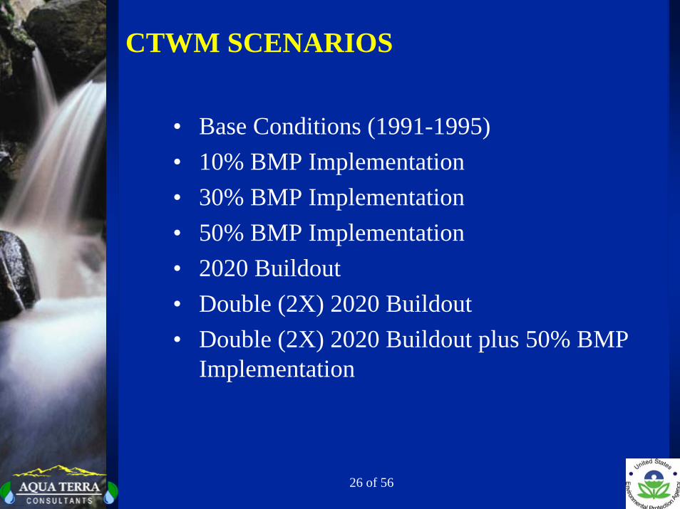
CTWM SCENARIOS

• Base Conditions (1991-1995)• 10% BMP Implementation• 30% BMP Implementation• 50% BMP Implementation• 2020 Buildout• Double (2X) 2020 Buildout• Double (2X) 2020 Buildout plus 50% BMP

Implementation

BMP MODULE

21 of 56

BMPs MODULE

• Built-in default parameter database with references

• Choice of using default numbers or user specified numbers

• Efficiency factors used for pollutant removal

• Removal efficiency input as constant or varying monthly

• Keeps track of pollutant removed

22 of 56

BMPs INCLUDED IN MODULE• Changes in land use acreage’s due to land use

planning/management

• Wet detention pond

• Dry detention pond

• Vegetated swales and filter strips(various widths)

• Stream buffers (25 feet and 100 feet)

• User specified sediment and pollutant (nitrogen, phosphorous, BOD, fecal coliform, metals - copper, cadmium, and zinc) load reductions

23 of 56

1

2

3

4

Land UseLand Use BMPBMP’’ss

Forest

Agriculture

Urban

ReceivingWater

Tributary 3

HSPF BMP MODULEHSPF BMP MODULE

Provided by CH2M Hill

24 of 56

SPECIFY BMP DETAILS

25 of 56

SET BMP EFFICIENCY INFORMATION

26 of 56

CTWM SCENARIOS

• Base Conditions (1991-1995)• 10% BMP Implementation• 30% BMP Implementation• 50% BMP Implementation• 2020 Buildout• Double (2X) 2020 Buildout• Double (2X) 2020 Buildout plus 50% BMP

Implementation

27 of 56

MODEL REPRESENTATION OF SCENARIOS

• Land use distributions for each model segment for the 2020 Buildout and 2X 2020 Buildout scenarios

• BMP removal efficiencies for urban and agricultural BMPs for all modeled constituents

• Model land use affected by the BMP implementation levels - 10%, 30%, 50%

28 of 56

REMOVAL EFFICIENCY VALUES USED IN THE CTWM

Constituent Removal Efficiency (%)

BODu 40%NOx 35%NH3 45%PO4 50%

Organic N 55%Organic P 55%Organic C 55%

29 of 56

PERCENT CHANGE IN AVERAGE ANNUAL LOADS DELIVERED TO LIS FOR EACH OF THE

CTWM SCENARIOS

ScenarioNPS Total NPS Total NPS Total

10% BMP Implementation -1.78 -0.48 -2.11 -0.39 -2.78 -1.07

30% BMP Implementation -5.70 -1.54 -6.62 -1.23 -8.99 -3.46

50% BMP Implementation -9.62 -2.59 -11.13 -2.07 -15.20 -5.852020 Buildout 1.38 0.37 1.38 0.26 1.72 0.66

Double 2(X) 2020 Buildout 2.56 0.69 2.53 0.47 3.09 1.19

Double 2(X) 2020 Buildout plus 50% BMP

Implemetation -7.90 -2.10 -9.40 -1.70 -13.40 -5.20

Total Nitrogen Total PhosphorusTotal Organic

Carbon

30 of 56

RELATIONSHIP BETWEEN PERCENT REDUCTION IN LOADS DELIVERED TO LIS AND PERCENT BMP

IMPLEMENTATION ON URBAN AND AGRICULTURAL LAND

0

5

10

15

10 30 50Percent BMP Implementation

Per

cent

Loa

d R

educ

tion

NPS TN

NPS TP

NPS TOC

(NPS+PS) TN

(NPS + PS) TP

(NPS + PS) TOC

NPS TOC

NPS TN

NPS TP

(NPS+PS) TOC

(NPS+PS) TN

(NPS+PS) TP

31 of 56

CTWM SUMMARY CONCLUSIONS• NPS reductions are relatively small, <15%, for all BMP

scenarios. However, this is consistent with expectations. Larger reductions would require increased area treated, increased removal efficiencies, or extending BMPs to other land uses.

• Largest reductions are for TOC, TP, and TN, in that order. Order is due to assumed removal efficiencies, loading rates, delivery processes, and sources.

• Significant differences in NPS impacts among CT Management Zones.

• Urban buildout scenarios show an almost linear impact on NPS loading rates. Increases are small due to limited potential forbuildout and relatively small state-wide urban fraction. Reasonable BMP implementation levels can offset growth impacts.

• CTWM and associated spreadsheet tool can be used for watershed and statewide planning-level assessments of BMPs and TMDL development.

SAMPLE TMDL CALCULATION

33 of 56

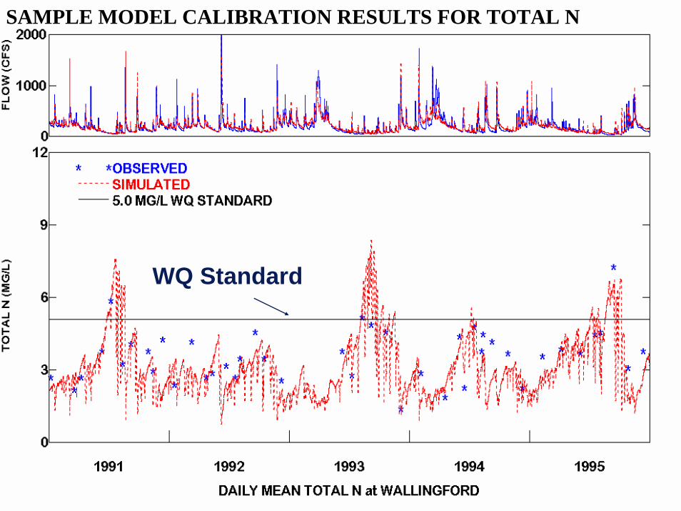
WQ Standard

SAMPLE MODEL CALIBRATION RESULTS FOR TOTAL N

34 of 56

SAMPLE: IMPACTS OF POINT SOURCE REDUCTION

WQ Standard

35 of 56

SAMPLE: IMPACTS OF NONPOINT SOURCE REDUCTION

WQ Standard

36 of 56

SAMPLE TMDL DETERMINATION

WQ Standard - 10% MOS

WQ Standard

37 of 56

SAMPLE TMDL DETERMINATION

WQ Standard - 10% MOS

WQ Standard

WLA + LA = TMDL1080 + 80 = 1160

lb/day lb/day lb/day

HSPF APPLICATION TO THEARROYO SIMI WATERSHED

VENTURA COUNTY, SOUTHERN CA

39 of 56

HSPF APPLICATION TO THE ARROYO SIMI WATERSHED VENTURA COUNTY, SOUTHERN CA

STUDY OBJECTIVES

• Develop hydrologic model of watershed• Assess potential urbanization impacts• Assess impacts of detention on flows and flood peaks• Provide tool for TMDLS, hydrograph modification,

urban stream erosion assessment (ongoing efforts)

40 of 56

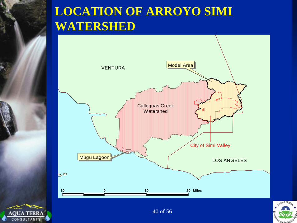
LOCATION OF ARROYO SIMI WATERSHED

Model Area

Mugu Lagoon

Calleguas CreekWatershed

#

City of Simi Valley

LOS ANGELES

VENTURA

10 0 10 20 Miles

41 of 56

REACH SEGMENTATION

42 of 56

SCENARIOS

• Natural, Pre-development

• 10% increase in urban fringe areas



• Detention Basins implemented with 50% increase in urban fringe areas

43 of 56

NATURAL CONDITIONS1. Removed all timeseries representing groundwater pumping

and dewatering, which contributed to the mainstem below Royal.

2. Removed all irrigation inputs for landscape watering.

3. Removed all detention and debris basins included within the Baseline setup, including Las Llagas, Runkle, Tapo 1 and 2, Erringer, and Sycamore. Oak Canyon basins were not constructed until after the calibration period, and therefore were not included in the Baseline model.

4. Eliminated any impervious areas, which were reassigned pervious land parameter values.

5. Assigned model parameters for the OPEN land use category to all the urban categories, except for physical characteristicssuch as slope, overland flow length, etc. which remained unchanged. This included parameters related to surface roughness, vegetal interception and ET, soil moisture storages (upper zone), and interflow.

44 of 56

LAND USE FOR BASELINE/CURRENT AND URBAN SEGMENT BOUNDARIES

�

�

�

��

�

��

��

��

��

��

��

�

��

��

��

�� !��

45 of 56

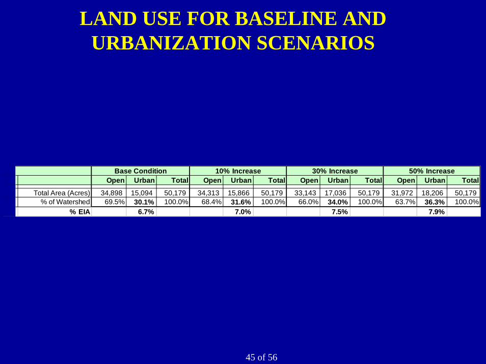
LAND USE FOR BASELINE AND URBANIZATION SCENARIOS

Open Urban Total Open Urban Total Open Urban Total Open Urban Total

Total Area (Acres) 34,898 15,094 50,179 34,313 15,866 50,179 33,143 17,036 50,179 31,972 18,206 50,179 % of Watershed 69.5% 30.1% 100.0% 68.4% 31.6% 100.0% 66.0% 34.0% 100.0% 63.7% 36.3% 100.0%

% EIA 6.7% 7.0% 7.5% 7.9%

50% IncreaseBase Condition 10% Increase 30% Increase

46 of 56

GENERALIZED LOCATIONS OF SCENARIO DETENTION BASINS

47 of 56

FLOW DURATION CURVES FOR MADERA USEP SITE FOR ALL SCENARIOS

48 of 56

STORM PEAK FLOWS (CFS) FOR ALL SCENARIOS BASED ON LOG PEARSON TYPE III ANALYSES

LocationReturn

Period, yr Natural Base+10% Urban

+30% Urban

+50% Urban

+50% Urban w

11 DBs Observed2 98 991 1031 1111 1195 514 12565 1389 2359 2425 2555 2691 1480 2646

10 4991 3776 3852 4004 4166 2628 39152 213 1677 1810 1856 1964 1044 21995 1867 4024 4225 4317 4491 2770 4418

10 5744 6515 6734 6869 7081 4741 64312 2 3 3 3 3 35 23 17 17 17 17 17

10 88 48 48 48 48 482 1 13 14 16 18 185 13 58 61 67 73 73

10 48 129 134 144 155 1552 2 71 79 93 107 1075 15 159 172 199 225 225

10 53 244 262 297 333 3332 2 63 69 83 96 245 15 140 152 176 200 70

10 49 216 232 264 296 126

Scenario

DRY CANYON

OAK CANYON

#1OAK

CANYON #2

ROYAL

MADERA

RUNKLE CANYON

49 of 56

WALNUT CREEK WATERSHED, IOWA

Agricultural Management Systems Evaluation Area (MSEA) Study

Joint USDA/ARS – EPA Effort

50 of 56

WALNUT CREEK WATERSHED, IOWA

51 of 56

52 of 56

ALTERNATE SCENARIOS FOR WALNUT CREEK

Baseline Conditions: Current Practices (i.e. MASTER Farming System # 2)

! Corn-soybean rotation! Fall Chisel plow, residues remain! Atrazine applied @ 0.4 kg a.i./ha, and

Metolachlor applied @ 1.12 kg a.i./ha! Corn land treated at 61% with Atrazine,

and 53% with Metolachlor! Spring fertilizer application @ 209 kg N/ha, on corn only (100%) (31 kgN/ha urea applied and

incorporated on 3/21, and 178 kgN/ha anhydrous NH 3 knifed in on 4/15)

Historical Conditions: Condition/Practices in 1960/70 (i.e. MASTER Farming System #1)

! Continuous corn (on all current cropland )! Fall Moldboard plow; no residues remain! Atrazine applied @ 3.36 kg a.i./ha; Metolachlor @ 2.24 kg a.i./ha! Corn area treated at same levels as Baseline, for both pesticides and N fertilizer! Fall fertilizer application @ 152 kgN/ha, spread and incorporated

Potential BMP Plan: Following Practices applied to Current (Baseline) Scenario

! MASTER Farming System No. 4: Crop Rotation - corn, soybeans, oats, meadow; 25% of cropland area planted in each crop.

! Riparian buffer strips & grass water ways - represented by an 80% reduction in sediment andsurface runoff pesticide and nitrogen loads (based on literature summary by Fawcett andChristiansen (1992)), and 40% reduction in shallow subsurface ( Interflow) loads.

! No change to Baseline pesticide application rates.

! Split fertilizer applications @ 140 kgN/ha: 25% at planting, 50% at 4 weeks, and 25% at 8weeks with anhydrous NH 3 knifed-in.

53 of 56

FREQUENCY ANALYSIS FOR ATRAZINE ANDMETOLACHLOR FOR ALL SCENARIOS

54 of 56

FREQUENCY ANALYSIS OF NITRATE FOR ALL SCENARIOS

55 of 56

LETHALITY ANALYSIS OF CHEMICAL CONCENTRATION DATA

56 of 56

PERCENT OF TIME DAILY PESTICIDE AND NO3-N CONCENTRATIONS ARE EXCEEDED FOR ALTERNATIVE WALNUT CREEK SCENARIOS(Based on 10-year simulations)

Chemical/Concentrations HISTORICAL BASELINE BMP

Atrazine0.1 ppb 89.2 33.9 14.01.0 ppb 36.1 4.6 0.23.0 ppb 19.6 0.4 0.0

Metolachlor0.05 ppb 68.1 40.3 14.40.1 ppb 54.7 27.3 9.61.0 ppb 11.7 3.4 0.01

NO33-N5.0 mg/l 90.4 97.3 82.7

10.0 mg/l 66.7 74.0 47.320.0 mg/l 31.2 39.7 12.0

lecture 16 -analysis of alternatives - us epa › sites › production › files › 2015-07 ›...

Documents