lecture 12 deleveraging and balance sheet effectswebfac/cromer/e210c_f11/lecture 12 slides... ·...

LECTURE 12 Deleveraging and Balance Sheet Effects

November 16, 2011

Economics 210c/236a Christina Romer Fall 2011 David Romer

I. INTRODUCTION

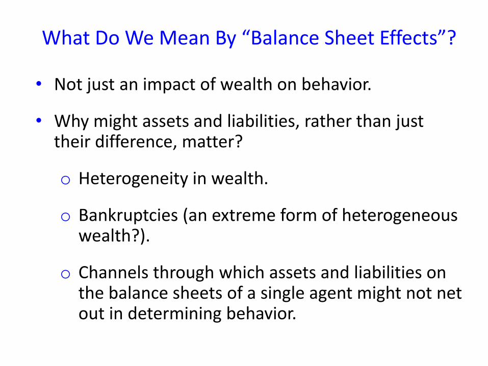
What Do We Mean By “Balance Sheet Effects”?

• Not just an impact of wealth on behavior.

• Why might assets and liabilities, rather than just their difference, matter?

o Heterogeneity in wealth.

o Bankruptcies (an extreme form of heterogeneous wealth?).

o Channels through which assets and liabilities on the balance sheets of a single agent might not net out in determining behavior.

II. RICHARD KOO, “JAPAN’S RECESSION”

Koo’s Hypotheses

• Japan’s poor macro performance is the result of balance sheet effects.

• In his view, why wasn’t it just the difference between assets and liabilities that mattered?

o In places, he seems to imply that the entire economy had negative net worth. But that can’t be right.

o His story appears to be one of heterogeneity: “many … firms had a negative net worth.”

Koo’s Hypotheses (cont.)

Balance sheet effects:

• Operate through AD, not AS.

• Operate through credit demand, not credit supply.

• Not only reduce demand, but make it less responsive to the interest rate.

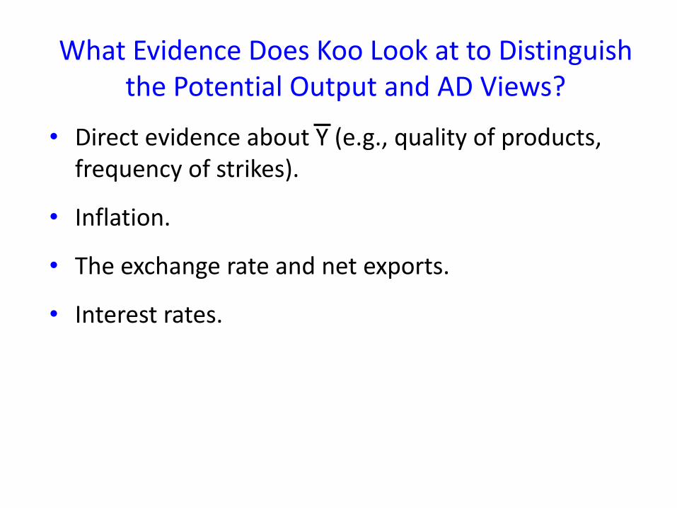
What Evidence Does Koo Look at to Distinguish the Potential Output and AD Views?

• Direct evidence about Y (e.g., quality of products, frequency of strikes).

• Inflation.

• The exchange rate and net exports.

• Interest rates.

What Evidence Does Koo Look at to Distinguish the Credit Supply and Credit Demand Views?

• Did firms that were able to issue debt?

• Did foreign banks enter?

• Were interest rates (real and nominal) high?

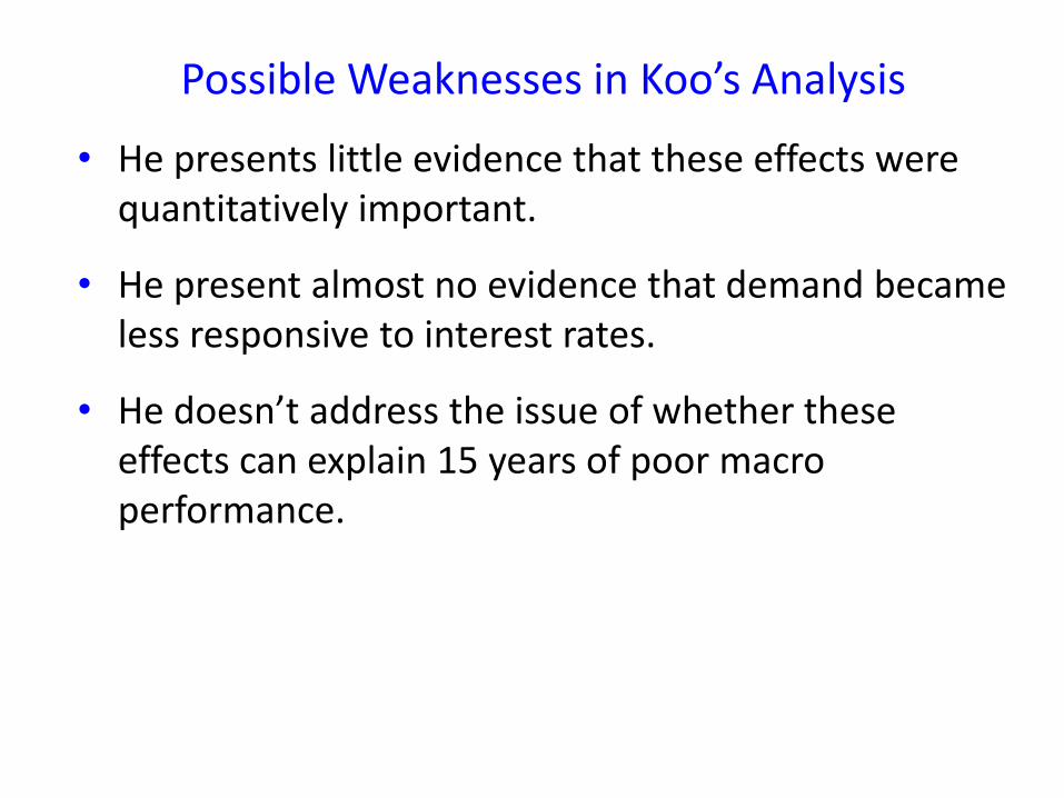
Possible Weaknesses in Koo’s Analysis

• He presents little evidence that these effects were quantitatively important.

• He present almost no evidence that demand became less responsive to interest rates.

• He doesn’t address the issue of whether these effects can explain 15 years of poor macro performance.

III. GAUTI B. EGGERTSSON AND PAUL KRUGMAN, “DEBT,

DELEVERAGING, AND THE LIQUIDITY TRAP: A

FISHER-MINSKY-KOO APPROACH”

Key Ingredients

• Two types of consumers – credit-constrained and unconstrained.

o As a result, the distribution of wealth, and not just its overall level, matters.

• Debt is denominated in nominal terms.

o Gives rise to endogenous redistributions.

• Central bank’s rule involves the inflation rate, not the price level.

o As a result, there’s no nominal anchor.

Case 1: Prices Are Flexible, Debt Is Denominated in Real Terms, and Monetary

Policy Is Targeting the Price Level

• Endowment economy.

• Half of households are impatient, borrow, and are constrained. Half of households are patient, save, and are unconstrained.

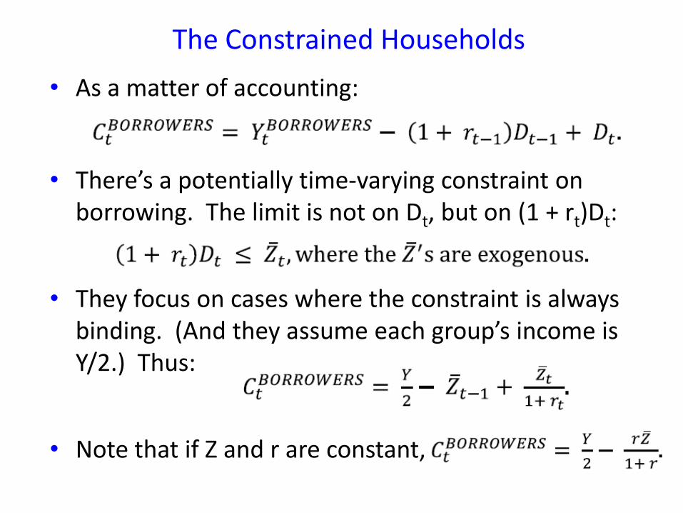
The Constrained Households

• As a matter of accounting:

• There’s a potentially time-varying constraint on borrowing. The limit is not on Dt, but on (1 + rt)Dt:

• They focus on cases where the constraint is always binding. (And they assume each group’s income is Y/2.) Thus:

• Note that if Z and r are constant,

The Unconstrained Households

• Utility:

• Euler equation:

Equilibrium

• rt adjusts so that

Their Focal Example

• Starting in some period, which we’ll call period 1, Z is permanently at some level below its previous value. Call the old value Z0 and the new value Z1.

• One can show that there is a steady state starting in period 2. The key feature of that steady state is that the consumption of the savers is constant and equal to

• In period 1:

Their Focal Example (cont.)

• Market clearing:

• Savers’ Euler equation:

• Putting all this together:

• Algebra yields:

Case 1 – Messages

• Deleveraging as a source of AD shocks.

• Government purchases still stimulate an economy affected by deleveraging.

• Tax cuts can stimulate an economy affected by deleveraging.

Question: Is there a tension between Eggertsson & Krugman’s MPC of 1 and Koo’s view that highly indebted agents will use additional resources only to pay down debt?

Case 2: Debt Is Denominated in Nominal Terms (Prices Are Flexible, and Monetary Policy Is

Targeting the Price Level)

• Same experiment as before, except debt is in nominal terms (and the fall in Z is unexpected).

• The price level before the shock is Pss (which is still the central bank’s long-run target).

• As a result, in period 1 borrowers have to repay Z0Pss/P1.

• Thus,

Case 2 (continued)

• Reasoning like that for case 1 yields

(*)

• At the zero lower bound,

• Algebra gives

Case 2 – Messages

• Having debt denominated in nominal terms magnifies the effects of deleveraging shocks.

• Expected inflation through a fall in the current price level and through a rise in the expected future price level are no longer equivalent.

What Happens When Monetary Policy Is Targeting the Inflation Rate?

• For a shock large enough to push the economy to the zero lower bound, if prices are flexible no equilibrium exists.

• If prices are sticky, equilibrium exists.

• With sticky prices:

o If debt is indexed, price flexibility has no effect on the real equilibrium.

o If debt is nominal, greater price flexibility increase the fall in output.

IV. MARTHA OLNEY, “AVOIDING DEFAULT: THE ROLE OF

CREDIT IN THE CONSUMPTION COLLAPSE OF 1930”

Key Features of Installment Debt in the 1920s

• It grew rapidly, and was substantial by the end of the decade.

• Down payments were high and contract durations were short.

• The penalty for default was that the seller could repossess the good, with no compensation for the excess of its value over what the buyer still owed.

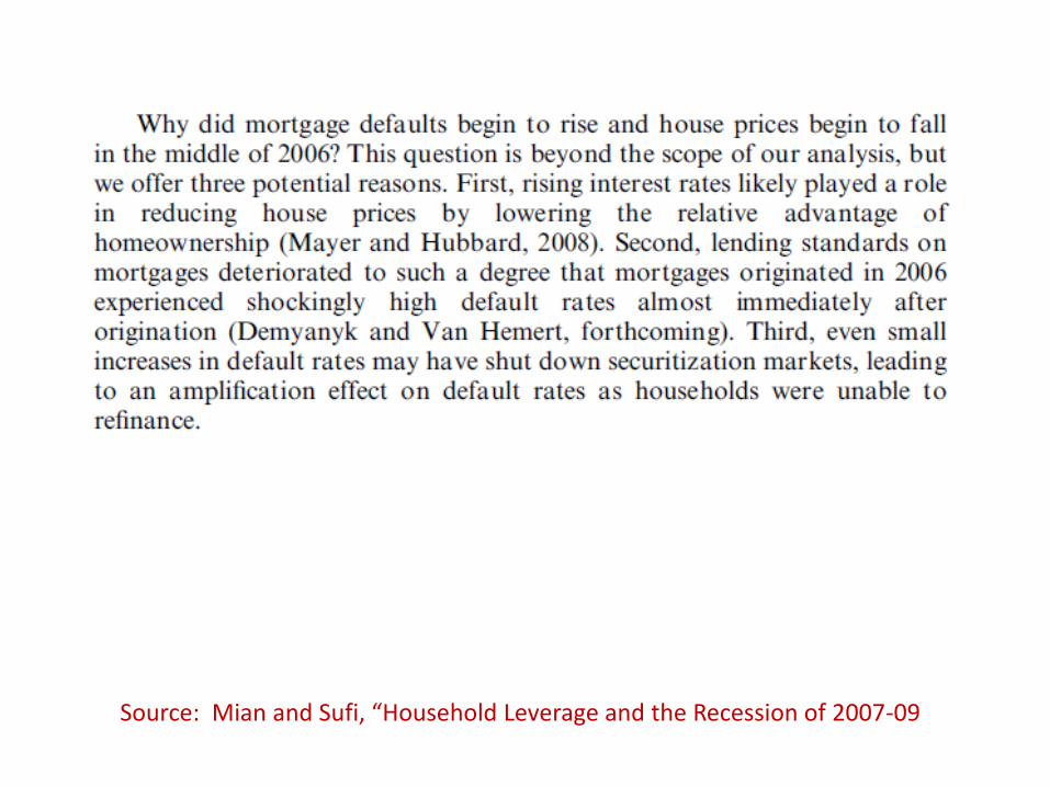
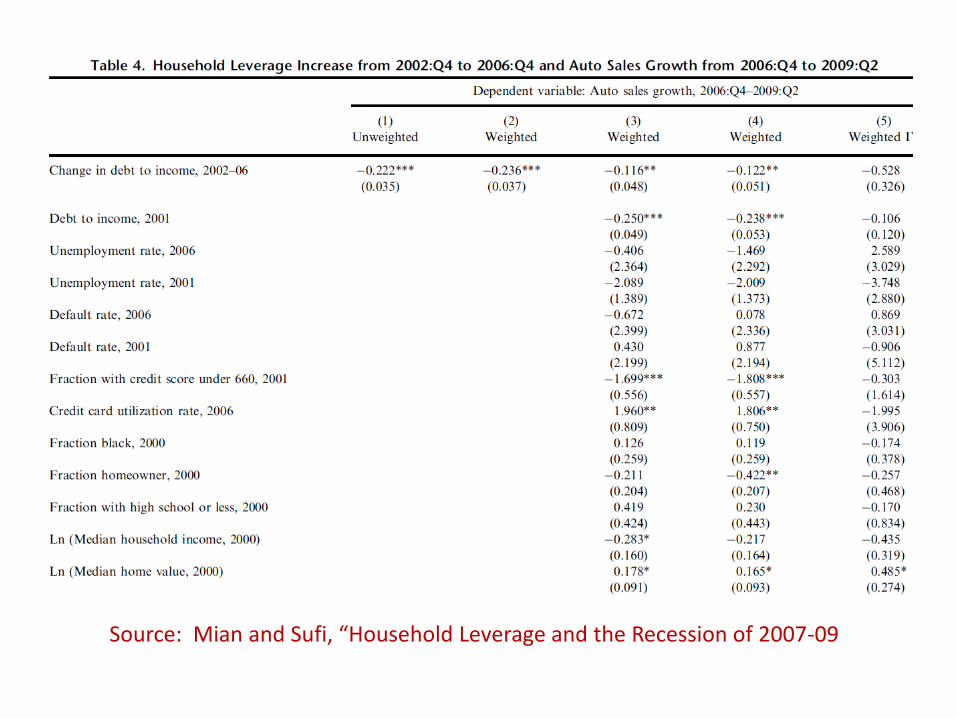
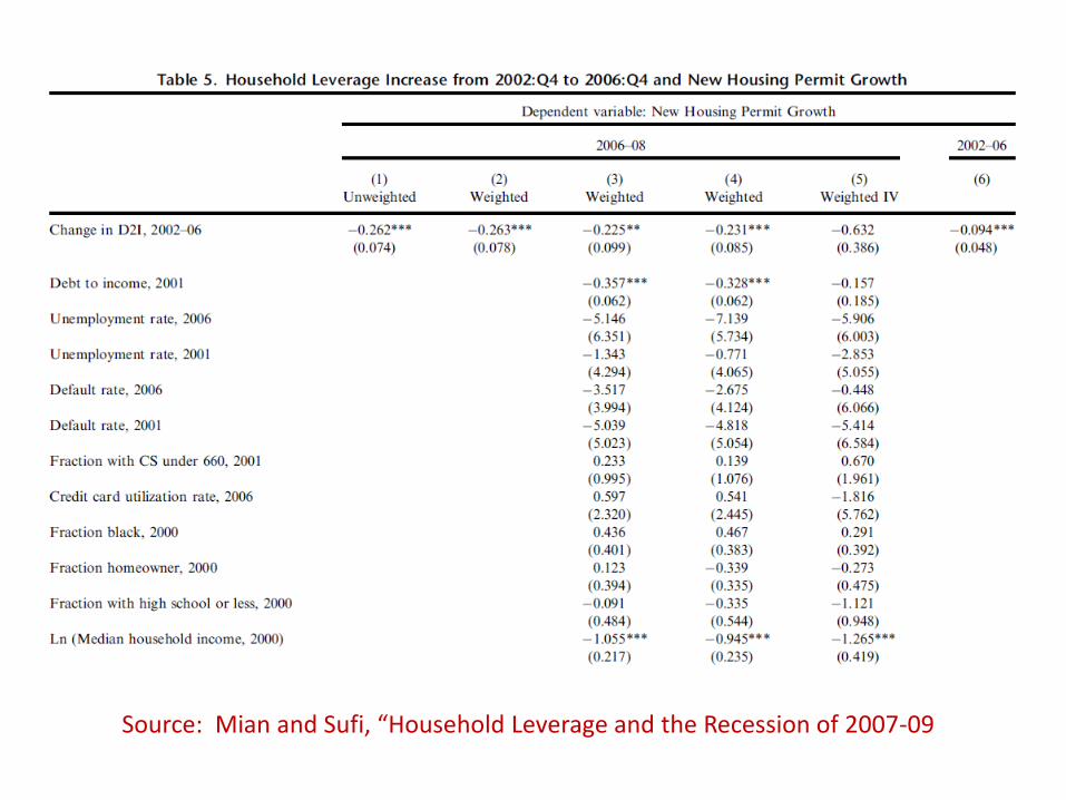
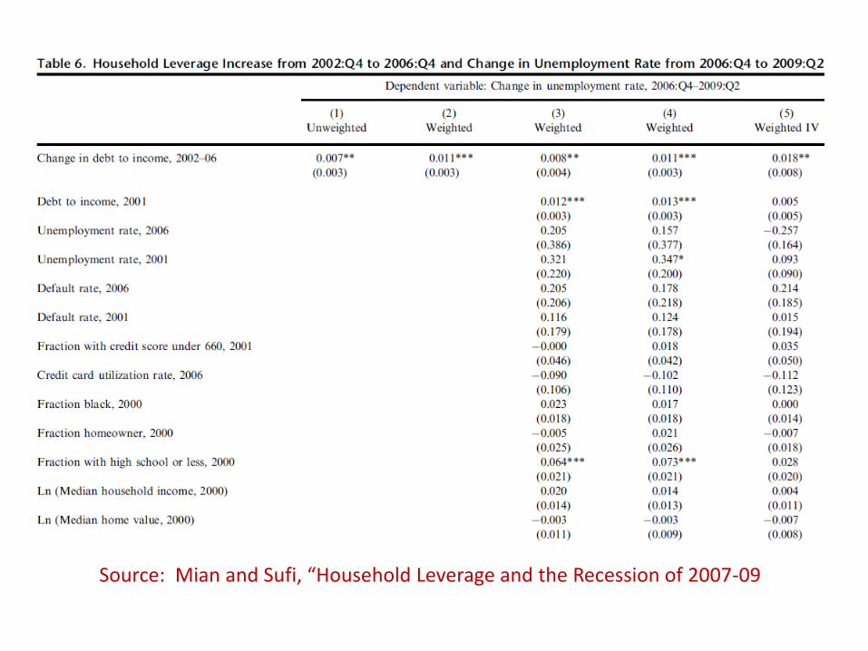
V. MIAN AND SUFI, “HOUSEHOLD LEVERAGE AND THE

RECESSION OF 2007-09”

Source: Mian and Sufi, “Household Leverage and the Recession of 2007-09

County-Level Data Set

• Equifax data by zip code

• Default rates

• Debt

• Credit score

• Credit card utilization

County-Level Data Set

• Income by zip code (IRS)

• House prices (FHFA, MSA level)

• Auto sales (Polk, registrations by county)

• New housing building permits (Census Bureau)

• Unemployment (QCEW, BLS)

• County employment and industrial composition (County Business Patterns, Census Bureau)

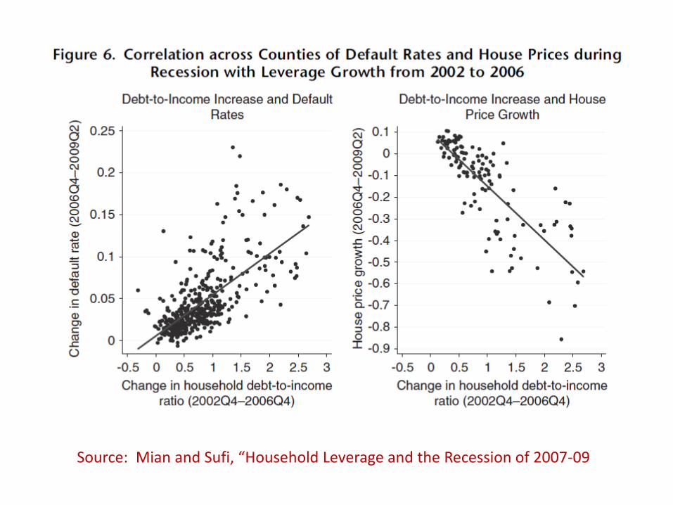
Key Explanatory Variable

• Growth in leverage from 2002Q4 to 2006Q4

• Is the growth in leverage the right variable?

• Do Mian and Sufi have a hypothesis for why leverage growth reduced consumer spending later on?

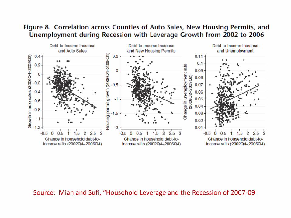
Outcome Variables

• House prices

• Default rate

• Auto sales

• Building permits

• Unemployment

Methodology

• Graphs of outcomes in high- and low-leverage counties.

• Scatter plots of outcome growth after 2006 and leverage growth before.

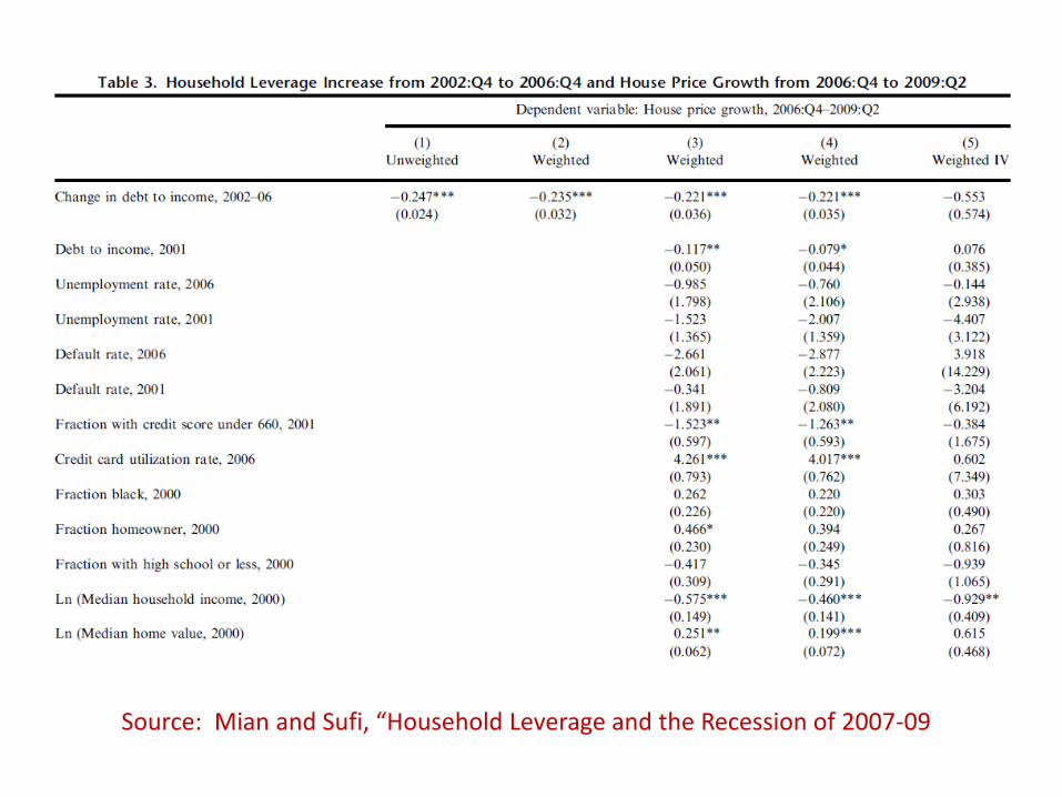
• First-difference regressions

First-Difference Regression Framework

• Economic Outcome: Change from 2006Q4 to 2009Q2

• Leverage Growth: Change from 2002Q4 to 2006Q4

• Control Variables: Set of cyclicality, demographic, and industrial composition measures

IV Regression Framework

• Housing supply inelasticity is a measure of how easy it was to increase housing in a county

• What omitted variable are they worried about?

Why do outcomes plummet in high- and low-leverage counties after 2008Q3?

• Mian and Sufi hypothesize credit-card utilization is another explanatory variable.

• Perhaps counties with higher credit-card utilization were more affected by the credit shock in the fall of 2008.

Could it be local banking conditions?

• Perhaps defaults caused local banks to have trouble.

• This trouble led to a decline in lending to county businesses.

lecture 12 deleveraging and balance sheet effectswebfac/cromer/e210c_f11/lecture 12 slides... ·...

Documents