Lecture 11 Tracking

Davide Scaramuzza

Lab Exercise 6 - Today

Room ETH HG E 33.1 from 14:15 to 16:00

Work description: Lukas-Kanade template tracking

Outline

• What is Tracking?

• Point tracking

• Template tracking

• Tracking by detection of local image features

What is tracking?

• Definition: Following of the motion of an image feature across an image sequence

Point Tracking

• Problem: given two images, estimate the motion of a pixel point from image 𝐼0 to image 𝐼1

Point Tracking

𝐼0(𝑥, 𝑦)

• Problem: given two images, estimate the motion of a pixel point from image 𝐼0 to image 𝐼1

Point Tracking

𝐼1(𝑥, 𝑦)

• Problem: given two images, estimate the motion of a pixel point from image 𝐼0 to image 𝐼1

• Two approaches exist, depending on the amount of motion between the frames

– Block-based methods

– Differential methods

Point Tracking

𝐼0(𝑥, 𝑦)

(𝑢, 𝑣): optical flow vector

Point Tracking • Consider the motion of the following corner

Point Tracking • Consider the motion of the following corner

Point Tracking with Block Matching • Search for the corresponding patch in a neighborhood around the point.

• Use SSD, SAD, or NCC to search for corresponding patches in a local neighborhood of the point. The search region is usually a 𝐷 × 𝐷 squared patch.

Search region

Patch to track

Point Tracking with Differential Methods

• Looks at the local brightness changes at the same location. No patch shift is performed!

Point Tracking with Differential Methods

• Looks at the local brightness changes at the same location. No patch shift is performed!

Point Tracking with Differential Methods

Assumptions:

1. Photo consistency

2. Temporal persistency

3. Spatial coherency

Photo Consistency

• A particular point in image 𝐼0 should have the same intensity as its corresponding point in image 𝐼1

Temporal Persistency (Short Base-Line)

• The motion between the two frames must be small

Spatial Coherency

• Neighboring pixels belonging to the same surface have similar motion

Applying the Spatial Coherency

• Assume that pixels in local neighborhood have the same motion (same 𝑢 and 𝑣) (usually, a square patch of 𝑛 × 𝑛 pixels is used)

• We want to find the motion vector (𝑢, 𝑣) that minimizes the Sum of Squared Differences (SSD):

𝑆𝑆𝐷 = (𝐼0 𝑥, 𝑦 − 𝐼1 𝑥 + 𝑢, 𝑦 + 𝑣 )2

≅ (𝐼0 𝑥, 𝑦 − 𝐼1 𝑥, 𝑦 − 𝐼𝑥𝑢 − 𝐼𝑦𝑣)2

= (∆𝐼 − 𝐼𝑥𝑢 − 𝐼𝑦𝑣)2

This is a simple quadratic function in two variables (𝑢, 𝑣)

Computing the Motion Vector

• To minimize the SSD, we differentiate E with respect to (𝑢, 𝑣) and equate it to zero

𝜕𝐸

𝜕𝑢= 0 ,

𝜕𝐸

𝜕𝑣= 0

𝜕𝐸

𝜕𝑢= 0 − 2 𝐼𝑥(∆𝐼 − 𝐼𝑥𝑢 − 𝐼𝑦𝑣) = 0

𝜕𝐸

𝜕𝑣= 0 − 2 𝐼𝑦 ∆𝐼 − 𝐼𝑥𝑢 − 𝐼𝑦𝑣 = 0

E= SSD= (∆𝐼 − 𝐼𝑥𝑢 − 𝐼𝑦𝑣)2

Computing the Motion Vector

• Linear system of two equations in two unknowns

• We can write them in matrix form:

𝜕𝐸

𝜕𝑢= 0 − 2 𝐼𝑥(∆𝐼 − 𝐼𝑥𝑢 − 𝐼𝑦𝑣) = 0

𝜕𝐸

𝜕𝑣= 0 − 2 𝐼𝑦 ∆𝐼 − 𝐼𝑥𝑢 − 𝐼𝑦𝑣 = 0

𝐼𝑥𝐼𝑥 𝐼𝑥𝐼𝑦

𝐼𝑥𝐼𝑦 𝐼𝑦𝐼𝑦

𝑢𝑣

=

𝐼𝑥∆𝐼

𝐼𝑦∆𝐼

𝑢𝑣

=

𝐼𝑥𝐼𝑥 𝐼𝑥𝐼𝑦

𝐼𝑥𝐼𝑦 𝐼𝑦𝐼𝑦

−1

𝐼𝑥∆𝐼

𝐼𝑦∆𝐼

M matrix Haven’t we seen this matrix already?

Recall Harris detector!

For M to be invertible, its determinant has to be non zero

2

1 and 2 are small

“Edge”

1 >> 2

“Edge”

2 >> 1

“Flat”

region 1

“Corner”

1 and 2 are large and

So is det(M)

𝑀 =

𝐼𝑥𝐼𝑥 𝐼𝑥𝐼𝑦

𝐼𝑥𝐼𝑦 𝐼𝑦𝐼𝑦

• In practice, det(M) should be as large as possible, which means that its eigenvalues should be large (i.e., not a flat region, not an edge) -> in practice, it should be a corner or more generally contain texture!

RR

2

11

0

0

Point Tracking Edge – Low texture – High texture

Simple 1D interpretation of Point Tracking

𝐼1(𝑥 + 𝑢)

Simple 1D interpretation of Point Tracking Sum of Squared Differences

u

𝐸 = (𝐼0 𝑥 − 𝐼1 𝑥 + 𝑢 )2

≅ 𝐼0 𝑥 − 𝐼1 𝑥 − 𝑢𝐼1′ 𝑥

2

𝑑𝐸

𝑑𝑢≅ −2𝐼1

′(𝑥)(𝐼0 𝑥 − 𝐼1 𝑥 − 𝑢𝐼1′ 𝑥 )

𝑢 ≅𝐼0 𝑥 − 𝐼1 𝑥

𝐼1′(𝑥)

𝐼1(𝑥 + 𝑢)

Simple 1D interpretation of Point Tracking Interpretation

𝑢 ≅𝐼0 𝑥 − 𝐼1 𝑥

𝐼′(𝑥)

𝐼1(𝑥 + 𝑢)

u

Aperture Problem • Consider the motion of the following corner

Aperture Problem • Consider the motion of the following corner

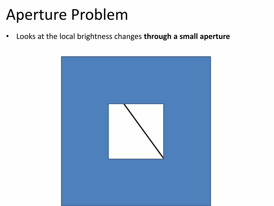
Aperture Problem • Looks at the local brightness changes through a small aperture

Aperture Problem • Looks at the local brightness changes through a small aperture

Aperture Problem • Looks at the local brightness changes through a small aperture

• We cannot always determine the motion direction -> Infinite motion solutions may exist!

• Solution?

Aperture Problem • Looks at the local brightness changes through a small aperture

• We cannot always determine the motion direction -> Infinite motion solutions may exist!

• Solution?: Increase aperture size!

• Optical flow or optic flow is the pattern of apparent motion of objects in a visual scene caused by the relative motion between the observer (an eye or a camera) and the scene

• Tracks the motion of every pixels (or a grid of pixels) between two consecutive frames

• For each pixel, a motion vector is computed: • Vector direction represents motion direction • Vector length represents the amount of movement

Application of Differential Methods: Optical Flow calculation

Optical Flow

[Tao et al., Eurographics 2012]

Optical Flow

[Tao et al., Eurographics 2012]

Optical Flow

[Tao et al., Eurographics 2012]

Optical Flow example

Optical flow issue: choosing the right patch size

Application to Corner Tracking

Color encodes motion direction

Block-based vs. Differential methods

• Block-based methods: search for the corresponding patch in a neighborhood of the point to be tracked. The search region is usually a square of 𝑛 × 𝑛 pixels. – Robust to large motions

– Can be computationally expensive (𝑛 × 𝑛 validations need to be made for a single point to track)

• Differential methods: – Works only for small motions (e.g., high frame rate). For larger motion, multi-

scale implementations are used but are more expensive

– Much more efficient than block-based methods. Thus, can be used to track the motion of every pixel in the image (i.e., optical flow). It avoids searching in the neighborhood of the point by analyzing the local intensity changes (i.e., differences) of an image patch at a specific location (i.e., no search is performed).

Outline

• What is Tracking?

• Point tracking

• Review of 2D image transformations and Jacobians

• Template tracking

• Tracking by detection of local image features

Transformations – 2D

Summary of displacement models (2D transformations)

• Translation

• Euclidean

• Affine

• Projective (homography)

𝑥′ = 𝑥 + 𝑎1 𝑦′ = 𝑦 + 𝑎2

𝑥′ = 𝑥𝑐𝑜𝑠(𝑎3) − 𝑦𝑠𝑖𝑛(𝑎3) + 𝑎1 𝑦′ = 𝑥𝑠𝑖𝑛(𝑎3) + 𝑦𝑐𝑜𝑠(𝑎3) + 𝑎2

𝑥′ = 𝑎1𝑥 + 𝑎3𝑦 + 𝑎5 𝑦′ = 𝑎2𝑥 + 𝑎4𝑦 + 𝑎6

𝑥′ =𝑎1𝑥 + 𝑎2𝑦 + 𝑎3𝑎7𝑥 + 𝑎8𝑦 + 1

𝑦′ =𝑎4𝑥 + 𝑎5𝑦 + 𝑎6𝑎7𝑥 + 𝑎8𝑦 + 1

Summary of displacement models (2D transformations)

• Translation

• Euclidean

• Affine

• Projective

𝑊 𝐱, 𝐩 =𝑥 + 𝑎1𝑦 + 𝑎2

=1 0 𝑎10 1 𝑎2

𝑥𝑦1

𝑊 𝐱,𝐩 =𝑥𝑐𝑜𝑠(𝑎3) − 𝑦𝑠𝑖𝑛(𝑎3) + 𝑎1𝑥𝑠𝑖𝑛(𝑎3) + 𝑦𝑐𝑜𝑠(𝑎3) + 𝑎2

=𝑐𝑎3 −𝑠𝑎3 𝑎1𝑠𝑎3 𝑐𝑎3 𝑎2

𝑥𝑦1

𝑊 𝐱,𝐩 =𝑎1𝑥 + 𝑎3𝑦 + 𝑎5𝑎2𝑥 + 𝑎4𝑦 + 𝑎6

=𝑎1 𝑎3 𝑎5𝑎2 𝑎4 𝑎6

𝑥𝑦1

Homogeneous coordinates

𝑊 𝒙 , 𝐩 =

𝑎1 𝑎2 𝑎3𝑎4 𝑎5 𝑎6𝑎7 𝑎8 1

𝑥𝑦1

We call the transformation Warping W 𝐱,𝐩 and p the set of parameters 𝑝 =(𝑎1, 𝑎2, … , 𝑎𝑛)

𝑊 𝐱, 𝐩 =1 0 𝑎10 1 𝑎2

𝑥𝑦1

𝑊 𝐱, 𝐩 =𝑐𝑎3 −𝑠𝑎3 𝑎1𝑠𝑎3 𝑐𝑎3 𝑎2

𝑥𝑦1

𝑊 𝐱, 𝐩 =𝑎1 𝑎3 𝑎5𝑎2 𝑎4 𝑎6

𝑥𝑦1

𝑊 𝒙 ,𝐩 =

𝑎1 𝑎2 𝑎3𝑎4 𝑎5 𝑎6𝑎7 𝑎8 1

𝑥𝑦1

𝑊 𝐱,𝐩 = λ𝑐𝑎3 −𝑠𝑎3 𝑎1𝑠𝑎3 𝑐𝑎3 𝑎2

𝑥𝑦1

Summary of displacement models (2D transformations)

Derivative and gradient

• Function: 𝑓 𝑥

• Derivative: 𝑓′ 𝑥 =𝑑𝑓

𝑑𝑥 , where 𝑥 is a scalar

• Function: 𝑓(𝑥1, 𝑥2, … , 𝑥𝑛 )

• Gradient: ∇𝑓(𝑥1, 𝑥2, … , 𝑥𝑛 )= 𝜕𝑓

𝜕𝑥1,𝜕𝑓

𝜕𝑥2, … ,

𝜕𝑓

𝜕𝑥𝑛

Jacobian

• 𝐹(𝑥1, 𝑥2, … , 𝑥𝑛 ) =𝑓1(𝑥1, 𝑥2, … , 𝑥𝑛 )

⋮𝑓𝑚(𝑥1, 𝑥2, … , 𝑥𝑛 )

Vector-valued function

Derivative?

𝐽 𝐹 = ∇𝐹 =

𝜕𝑓1𝜕𝑥1

, … ,𝜕𝑓1𝜕𝑥𝑛

⋮𝜕𝑓𝑚𝜕𝑥1

, … ,𝜕𝑓𝑚𝜕𝑥𝑛

Carl Gustav Jacob (1804-1851)

Displacement-model Jacobians

• Translation

• Euclidean

• Affine

𝑊 𝐱, 𝐩 =𝑥 + 𝑎1𝑦 + 𝑎2

𝑊 𝐱, 𝐩 =𝑥𝑐𝑜𝑠(𝑎3) − 𝑦𝑠𝑖𝑛(𝑎3) + 𝑎1𝑥𝑠𝑖𝑛(𝑎3) + 𝑦𝑐𝑜𝑠(𝑎3) + 𝑎2

𝑊 𝐱, 𝐩 =𝑎1𝑥 + 𝑎3𝑦 + 𝑎5𝑎2𝑥 + 𝑎4𝑦 + 𝑎6

∇𝑊𝑝

∇𝑊𝑝=

𝜕𝑊1

𝜕𝑎1

𝜕𝑊1

𝜕𝑎2𝜕𝑊2

𝜕𝑎1

𝜕𝑊2

𝜕𝑎2

=1 00 1

𝑝 = (𝑎1, 𝑎2, … , 𝑎𝑛)

∇𝑊𝑝=1 0 −𝑥𝑠𝑖𝑛(𝑎3) − 𝑦𝑐𝑜𝑠(𝑎3)0 1 𝑥𝑐𝑜𝑠(𝑎3) − 𝑦𝑠𝑖𝑛(𝑎3)

∇𝑊𝑝=𝑥 0 𝑦0 𝑥 0

0 1 0𝑦 0 1

Outline

• What is Tracking?

• Point tracking

• Review of 2D image transformations and Jacobians

• Template tracking: Lucas-Kanade algorithm

• Tracking by detection of local image features

Template tracking

Definition: follow a template image in a video sequence by estimating the warp

Template image

The Lucas-Kanade tracker

B. D. Lucas and T. Kanade (1981), An iterative image registration technique with an application to stereo vision. Proceedings of Imaging Understanding Workshop, pages 121--130

Template warping

• Given the template image 𝑇(𝐱)

• Take all pixels from the template image 𝑇(𝐱) and warp them using the function 𝑊 𝐱, 𝐩 parameterized in terms of parameters 𝐩

Template image

𝑇(𝐱)

𝑊 𝐱, 𝐩

warp

𝐼(𝑥 )

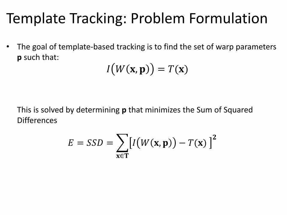
Template Tracking: Problem Formulation

• The goal of template-based tracking is to find the set of warp parameters p such that: This is solved by determining p that minimizes the Sum of Squared Differences

𝐼 𝑊 𝐱, 𝐩 = 𝑇(𝐱)

𝐸 = 𝑆𝑆𝐷 = 𝐼 𝑊 𝐱, 𝐩 − 𝑇(𝐱) 𝟐

𝐱∈𝐓

Assumptions

• No errors in the template image boundaries: only the appearance of the object to be tracked appears in the template image

• No occlusion: the entire template is visible in the input image

• Brightness constancy assumption: the intensity of the object appearance is always the same.

The Lucas-Kanade tracker

• Uses the Gauss-Newton method for minimization, that is:

– Applies a first-order approximation of the warp

– Attempts to minimize the SSD iteratively

Derivation of the Lucas-Kanade algorithm

• Assume that an initial estimate of p is known. Then, we want to find the increment ∆𝐩 that minimizes

• First-order Taylor approximation of 𝐼 𝑊 𝐱, 𝐩 + ∆𝐩 yelds to:

𝐸 = 𝐼 𝑊 𝐱, 𝐩 − 𝑇(𝐱) 𝟐

𝐱∈𝐓

𝐼 𝑊 𝐱, 𝐩 + ∆𝐩 − 𝑇(𝐱) 𝟐

𝐱∈𝐓

𝐼 𝑊 𝐱, 𝐩 + ∆𝐩 ≅ 𝐼 𝑊 𝐱, 𝐩 +𝛻𝐼𝜕𝑊

𝜕𝐩∆𝐩

𝛻𝐼 = 𝐼𝑥, 𝐼𝑦 = Image gradient evaluated at 𝑊(𝐱, 𝐩) Jacobian of the warp 𝑊(𝐱, 𝐩)

How do I get the initial estimate?

Derivation of the Lucas-Kanade algorithm

• By replacing 𝐼 𝑊 𝐱, 𝐩 + ∆𝐩 with its 1st order approximation, we get

• How do we minimize it?

• We differentiate E with respect to ∆𝐩 and we equate it to zero, i.e.,

𝐸 = 𝐼 𝑊 𝐱, 𝐩 + ∆𝐩 − 𝑇(𝐱) 𝟐

𝐱∈𝐓

𝐸 = 𝐼 𝑊 𝐱, 𝐩 +𝛻𝐼𝜕𝑊

𝜕𝐩∆𝐩 − 𝑇(𝐱)

𝟐

𝐱∈𝐓

𝜕𝐸

𝜕∆𝐩= 0

Derivation of the Lucas-Kanade algorithm

𝜕𝐸

𝜕∆𝐩= 2 𝛻𝐼

𝜕𝑊

𝜕𝐩

T

𝐼 𝑊 𝐱, 𝐩 +𝛻𝐼𝜕𝑊

𝜕𝐩∆𝐩 − 𝑇(𝐱)

𝐱∈𝐓

𝜕𝐸

𝜕∆𝐩= 0

2 𝛻𝐼𝜕𝑊

𝜕𝐩

T

𝐼 𝑊 𝐱, 𝐩 +𝛻𝐼𝜕𝑊

𝜕𝐩∆𝐩 − 𝑇(𝐱)

𝐱∈𝐓

= 0

𝐸 = 𝐼 𝑊 𝐱, 𝐩 +𝛻𝐼𝜕𝑊

𝜕𝐩∆𝐩 − 𝑇(𝐱)

𝟐

𝐱∈𝐓

Derivation of the Lucas-Kanade algorithm

∆𝐩 = 𝐻−1 𝛻𝐼𝜕𝑊

𝜕𝐩

T

𝑇 𝐱 − 𝐼 𝑊 𝐱, 𝐩

𝐱∈𝐓

=

𝐻 = 𝛻𝐼𝜕𝑊

𝜕𝐩

T

𝛻𝐼𝜕𝑊

𝜕𝐩𝐱∈𝐓

Second moment matrix (Hessian) of the warped image

What does H look like when the warp is a pure translation?

Lucas-Kanade algorithm

1. Warp 𝐼(𝐱) with 𝑊(𝐱, 𝐩) 𝐼 𝑊 𝐱, 𝐩

2. Compute the error: subtract 𝐼 𝑊 𝐱, 𝐩 from 𝑇(𝐱)

3. Compute warped gradients: 𝛻𝐼 = 𝐼𝑥, 𝐼𝑦 , evaluated at 𝑊(𝐱, 𝐩)

4. Evaluate the Jacobian of the warping: 𝜕𝑊

𝜕𝐩

5. Compute steepest descent: 𝛻𝐼𝜕𝑊

𝜕𝐩

6. Compute Inverse Hessian: 𝐻−1 = 𝛻𝐼𝜕𝑊

𝜕𝐩

T𝛻𝐼

𝜕𝑊

𝜕𝐩𝐱∈𝐓

−1

7. Multiply steepest descend with error: 𝛻𝐼𝜕𝑊

𝜕𝐩

T𝑇 𝐱 − 𝐼 𝑊 𝐱,𝐩𝐱∈𝐓

8. Compute ∆𝐩

9. Update parameters: 𝐩 𝐩 + ∆𝐩

10. Repeat until ∆𝐩 < 𝜺

∆𝐩 = 𝐻−1 𝛻𝐼𝜕𝑊

𝜕𝐩

T

𝑇 𝐱 − 𝐼 𝑊 𝐱, 𝐩

𝐱∈𝐓

Lucas-Kanade algorithm

B. D. Lucas and T. Kanade (1981), An iterative image registration technique with an application to stereo vision. Proceedings of Imaging Understanding Workshop, pages 121--130

∆𝐩 = 𝐻−1 𝛻𝐼𝜕𝑊

𝜕𝐩

T

𝑇 𝐱 − 𝐼 𝑊 𝐱, 𝐩

𝐱∈𝐓

6x1

6x6

Lucas-Kanade algorithm

B. D. Lucas and T. Kanade (1981), An iterative image registration technique with an application to stereo vision. Proceedings of Imaging Understanding Workshop, pages 121--130

∆𝐩 = 𝐻−1 𝛻𝐼𝜕𝑊

𝜕𝐩

T

𝑇 𝐱 − 𝐼 𝑊 𝐱, 𝐩

𝐱∈𝐓

6x1

6x6

Lucas-Kanade algorithm

B. D. Lucas and T. Kanade (1981), An iterative image registration technique with an application to stereo vision. Proceedings of Imaging Understanding Workshop, pages 121--130

∆𝐩 = 𝐻−1 𝛻𝐼𝜕𝑊

𝜕𝐩

T

𝑇 𝐱 − 𝐼 𝑊 𝐱, 𝐩

𝐱∈𝐓

6x1

6x6

What is the size? 𝟐𝒏 × 𝟔𝒏

𝒏 × 𝟐𝒏

Why does it look like that?

𝜕𝑊

𝜕𝐩=

𝑥 0 𝑦

0 𝑥 0 0 1 0

𝑦 0 1

Lucas-Kanade algorithm

B. D. Lucas and T. Kanade (1981), An iterative image registration technique with an application to stereo vision. Proceedings of Imaging Understanding Workshop, pages 121--130

∆𝐩 = 𝐻−1 𝛻𝐼𝜕𝑊

𝜕𝐩

T

𝑇 𝐱 − 𝐼 𝑊 𝐱, 𝐩

𝐱∈𝐓

6x1

6x6

Why does it look like that?

What is the size? 𝟐𝒏 × 𝟔𝒏

𝒏 × 𝟐𝒏

What’s its size?

nx6n

𝜕𝑊

𝜕𝐩=

𝑥 0 𝑦

0 𝑥 0 0 1 0

𝑦 0 1

Lucas-Kanade algorithm

B. D. Lucas and T. Kanade (1981), An iterative image registration technique with an application to stereo vision. Proceedings of Imaging Understanding Workshop, pages 121--130

∆𝐩 = 𝐻−1 𝛻𝐼𝜕𝑊

𝜕𝐩

T

𝑇 𝐱 − 𝐼 𝑊 𝐱, 𝐩

𝐱∈𝐓

6x1

6x6

Why does it look like that?

What is the size? 𝟐𝒏 × 𝟔𝒏

𝒏 × 𝟐𝒏

What’s its size?

nx6n

𝜕𝑊

𝜕𝐩=

𝑥 0 𝑦

0 𝑥 0 0 1 0

𝑦 0 1

Lucas-Kanade algorithm

B. D. Lucas and T. Kanade (1981), An iterative image registration technique with an application to stereo vision. Proceedings of Imaging Understanding Workshop, pages 121--130

𝜕𝑊

𝜕𝐩=

𝑥 0 𝑦

0 𝑥 0 0 1 0

𝑦 0 1

Why does it look like that?

What is the size? 𝟐𝒏 × 𝟔𝒏

What’s its size?

∆𝐩 = 𝐻−1 𝛻𝐼𝜕𝑊

𝜕𝐩

T

𝑇 𝐱 − 𝐼 𝑊 𝐱, 𝐩

𝐱∈𝐓

nx6n

𝒏 × 𝟐𝒏

6x1

6x6 6x1

Lucas-Kanade algorithm: Discussion

Lucas-Kanade follows a predict-correct cycle

• A prediction 𝐼 𝑊 𝐱, 𝐩 of the warped image is computed from an initial

estimate

• The correction parameter ∆𝐩 is computed as a function of the error

𝑇 𝐱 − 𝐼 𝑊 𝐱, 𝐩 between the prediction and the template

• The larger this error, the larger the correction applied

predict correct

Lucas-Kanade algorithm: Discussion

• How to get the initial estimate p?

• When does the Lucas-Kanade fail?

– If the initial estimate is too far, then the linear approximation does not longer hold -> solution?

• Pyramidal implementations (see next slide)

• Other problems:

– Deviations from the mathematical model: object deformations, illumination changes, etc.

– Occlusions

– Due to these reasons, tracking may drift -> solution?

• Update the template with the last image

Coarse-to-fine estimation

image I

pI(W) warp refine

p Δp

+

Pyramid of image I Pyramid of image T

image T u=10 pixels

u=5 pixels

u=1.25 pixels

u=2.5 pixels

image T

Coarse-to-fine estimation

I I(W) T warp refine

inp

p

+

I I(W) T warp refine

p

p+

I

pyramid construction

I I(W) T warp refine

p+

T

pyramid construction

outp

Generalization of Lucas-Kanade

• The same concept (predict/correct) can be applied to tracking of 3D object (in this case, what is the transformation to etimate? What is the template?)

Generalization of Lucas-Kanade

• The same concept (predict/correct) can be applied to tracking of 3D object (in this case, what is the transformation to etimate? What is the template?)

• In order to deal with wrong prediction, it can be implemented in a Particle-Filter fashion (using multiple hipotheses that need to be validated)

Outline

• What is Tracking?

• Review of 2D image transformations and Jacobians

• Point tracking

• Template tracking

• Tracking by detection of local image features

Tracking by detection of local image features

Step 1: Keypoint detection and matching • invariant to scale, rotation, or perspective

Template image with the object to detect Current test image

Tracking by detection of local image features

Step 1: Keypoint detection and matching • invariant to scale, rotation, or perspective

Template image with the object to detect Current test image

Tracking by detection of local image features

Step 1: Keypoint detection and matching • invariant to scale, rotation, or perspective

Step 2: Geometric verification (RANSAC)

Template image with the object to detect Current test image

Tracking by detection of local image features

Tracking issues

• How to segment the object to track from background?

• How to initialize the warping?

• How to handle occlusions

• How to handle illumination changes and non modeled effects?

References

• Chapter 8.2, Richard Szeliski, "Computer Vision: Algorithms and Application".

• Original paper: B. D. Lucas and T. Kanade (1981), An iterative image registration technique with an application to stereo vision. Proceedings of Imaging Understanding Workshop, pages 121—130

• Baker, Matthews, “Lucas‐Kanade 20 Years On: A Unifying Framework”, IJCV, 2004.

Implementations

• OpenCV implementation : http://docs.opencv.org/modules/video/doc/motion_analysis_and_object_tracking.html?highlight=lucas%20kanade

• Some Matlab implementation:

– Lucas Kanade with Pyramid http://www.mathworks.com/matlabcentral/fileexchange/30822

– Affine tracking: http://www.mathworks.com/matlabcentral/fileexchange/24677‐lucas‐kanade‐affine‐template‐tracking http://vision.eecs.ucf.edu/Code/Optical_Flow/Lucas%20Kanade.zip