lecture 11: non-linear dynamical systems: part...
TRANSCRIPT

The application of non-linear systems analysis to understand the elementary response of Drosophila photoreceptor cells to light.
Lecture 11: Non-linear dynamical systems: Part 3
R. Ranganathan Green Center for Systems Biology, ND11.120E
Boris Shraiman KITP, UCSB
Henri Poincare 1854 - 1912
Edward Lorenz 1917-2008
Robert May 1936 -
Alain Pumir CNRS, ENS de Lyon

So, today we study a real case of a biological non-linear dynamical system.
Linear
Nonlinear
n = 1
n = 2 or 3
n >> 1
continuum
exponential growth and decay
single step conformational change
fluorescence emission
pseudo first order kinetics
fixed points
bifurcations, multi stability
irreversible hysteresis
overdamped oscillators
second order reaction kinetics
linear harmonic oscillators
simple feedback control
sequences of conformational change
anharmomic oscillators
relaxation oscillations
predator-prey models
van der Pol systems
Chaotic systems
electrical circuits
molecular dynamics
systems of coupled harmonic oscillators
equilibrium thermodynamics
diffraction, Fourier transforms
systems of non-linear oscillators
non-equilibrium thermodynamics
protein structure/function
neural networks
the cell
ecosystems
Diffusion
Wave propagation
quantum mechanics
viscoelastic systems
Nonlinear wave propagation
Reaction-diffusion in dissipative systems
Turbulent/chaotic flows
adapted from S. Strogatz

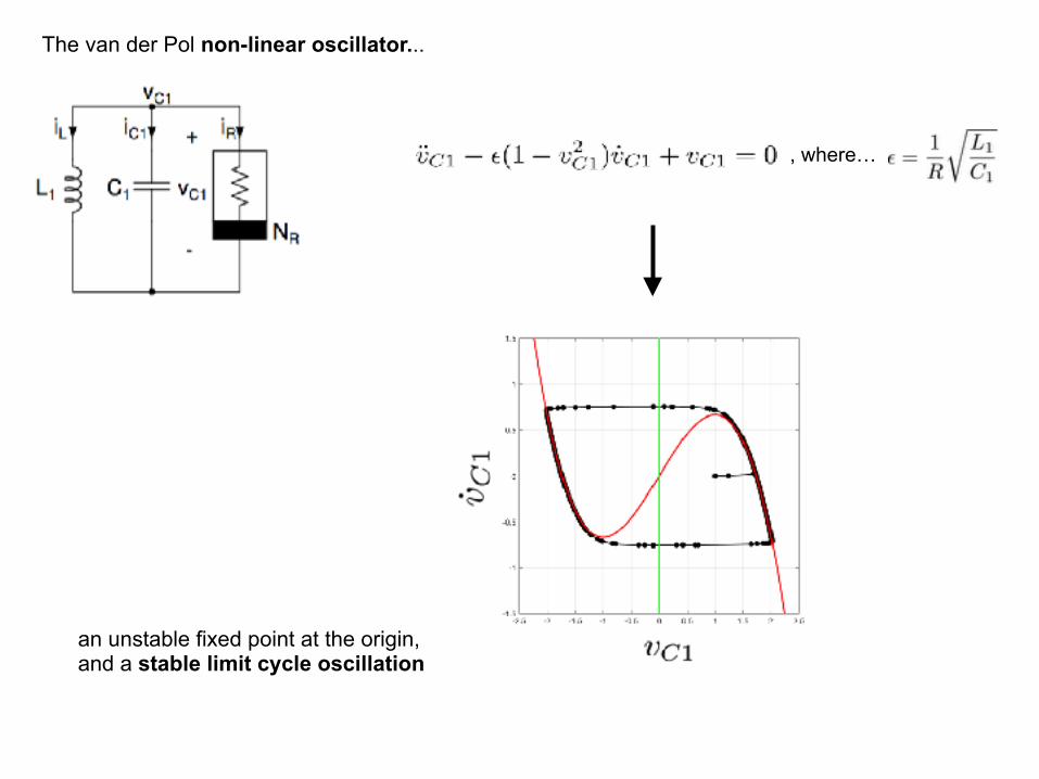
The van der Pol non-linear oscillator...
, where…
The van der Pol non-linear oscillator...
, where…
an unstable fixed point at the origin, and a stable limit cycle oscillation

The van der Pol non-linear oscillator...
, where…
the switch from slow to fast flow…

The neuronal action potential…a slight variation on the van der Pol oscillator…
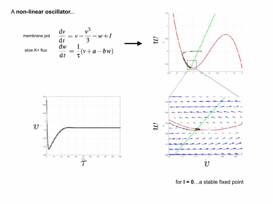
A non-linear oscillator...

A non-linear oscillator...
this is essentially the van der Pol oscillator, with one difference….
Fitzhugh-Nagumo (1962)
membrane pot
slow K+ flux

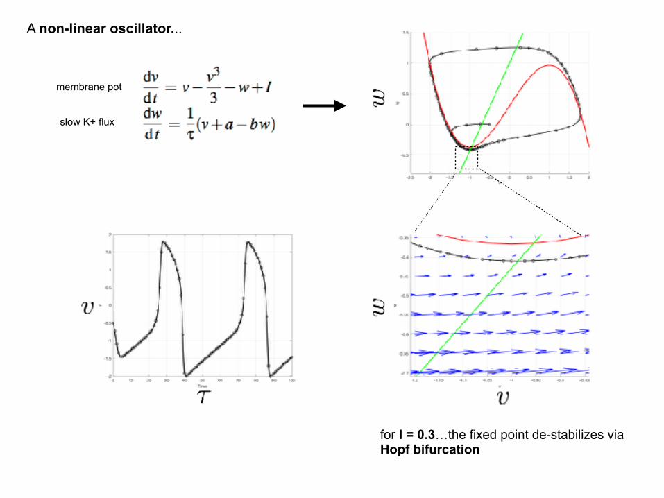
A non-linear oscillator...
the linear term to the w nullcline provides for thresholded oscillation….
membrane pot
slow K+ flux
A non-linear oscillator...
for I = 0…a stable fixed point
membrane pot
slow K+ flux

A non-linear oscillator...
membrane pot
slow K+ flux
for I = 0.1…a stable fixed point, but a transient oscillation…

A non-linear oscillator...
membrane pot
slow K+ flux
for I = 0.2…a stable fixed point, but a larger transient oscillation…
A non-linear oscillator...
membrane pot
slow K+ flux
for I = 0.3…the fixed point de-stabilizes via Hopf bifurcation

A non-linear oscillator...
membrane pot
slow K+ flux
This provides for a thresholded firing of the action potential…

A non-linear oscillator...
the linear term to the w nullcline provides for thresholded oscillation….
membrane pot
slow K+ flux

Φ(x,y,t)
200 ms
1 nA
The Drosophila eye
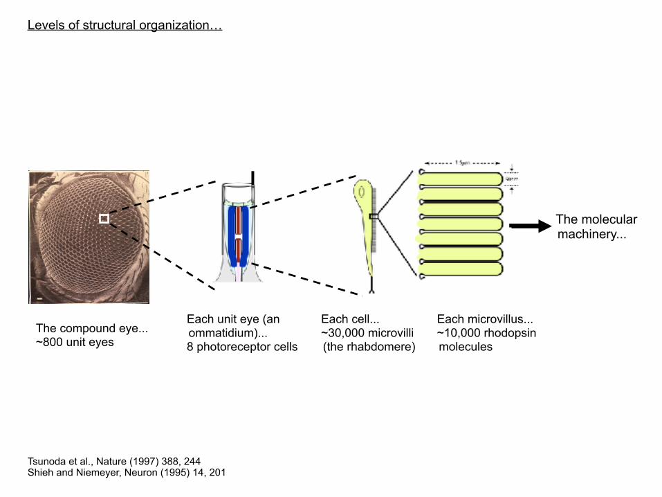
Tsunoda et al., Nature (1997) 388, 244 Shieh and Niemeyer, Neuron (1995) 14, 201
Levels of structural organization…
The molecular machinery...
The compound eye... ~800 unit eyes
Each unit eye (an ommatidium)... 8 photoreceptor cells
Each cell... ~30,000 microvilli (the rhabdomere)
Each microvillus... ~10,000 rhodopsin molecules


200 ms
1 nA
The Macroscopic Impulse Response:
A statistical superposition of quantal responses. This response is the bump latency distribution convolved with the average bump size and shape.
The Single Photon Response (Quantum Bump):
Stochastic electrical response to the absorption of a single photon. Parameters: size, shape, latency of occurrence, and a refractory period.

Linearity at the cellular level...
Henderson and Hardie, J.Physiol. (2000) 524.1, 179

R M
MArr
Gq(αβγ)-GDP
Gqα-GTP + Gβγ
PLC-β PLC-β*
[ninaE]
[arr1] [arr2]
[dgq] [gbe]
[norpA]
PIP2 IP3 + DAG
[trp] [trpl]
Na+Na+/Ca2+
ePKC, CamK[inaC]
++
-
480nm
580nm

Calcium-dependence...
the macroscopic response.. the quantum bump....
Henderson and Hardie, J. Physiol. (2000) 524, 179
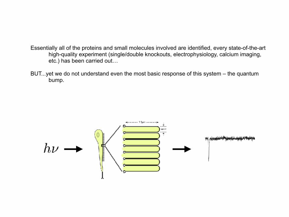
Essentially all of the proteins and small molecules involved are identified, every state-of-the-art high-quality experiment (single/double knockouts, electrophysiology, calcium imaging, etc.) has been carried out…
BUT...yet we do not understand even the most basic response of this system – the quantum bump.
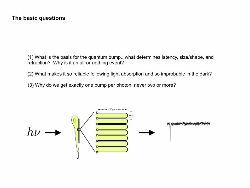
The basic questions
(1) What is the basis for the quantum bump...what determines latency, size/shape, and refraction? Why is it an all-or-nothing event?
(2) What makes it so reliable following light absorption and so improbable in the dark?
(3) Why do we get exactly one bump per photon, never two or more?

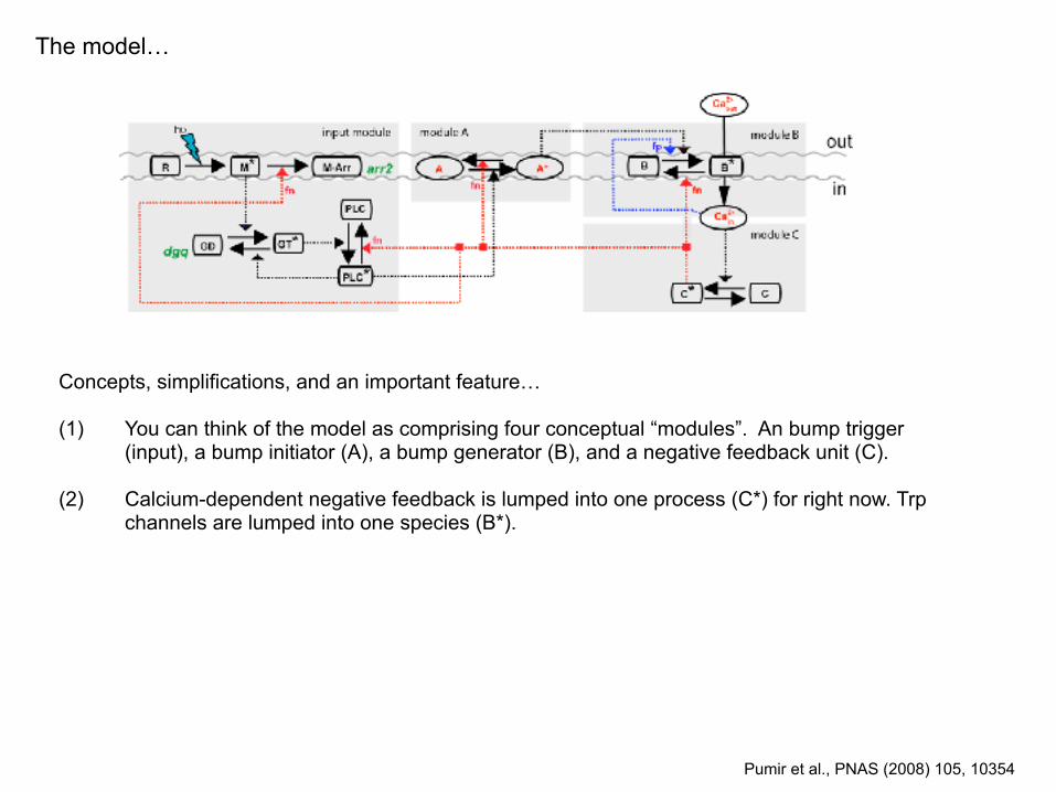
The model…
Concepts, simplifications, and an important feature…
(1) You can think of the model as comprising four conceptual “modules”. An bump trigger (input), a bump initiator (A), a bump generator (B), and a negative feedback unit (C).
Pumir et al., PNAS (2008) 105, 10354
The model…
Concepts, simplifications, and an important feature…
(1) You can think of the model as comprising four conceptual “modules”. An bump trigger (input), a bump initiator (A), a bump generator (B), and a negative feedback unit (C).
(2) Calcium-dependent negative feedback is lumped into one process (C*) for right now. Trp channels are lumped into one species (B*).
Pumir et al., PNAS (2008) 105, 10354

The model…
Concepts, simplifications, and an important feature…
(1) You can think of the model as comprising four conceptual “modules”. An bump trigger (input), a bump initiator (A), a bump generator (B), and a negative feedback unit (C).
(2) Calcium-dependent negative feedback is lumped into one process (C*) for right now. Trp channels are lumped into one species (B*).
(2) Some known molecules (e.g. M* inactivation, and InaD) are represented implicitly in the model.
(3) System operates at the stochastic limit (1 M*, 1-5 G*, 1-5 PLC*…15-25 B*), so requires stochastic simulation methods (numbers, not concentrations of species). We will describe the method for computational simulation of the reaction dynamics shortly...
Pumir et al., PNAS (2008) 105, 10354

The model…mathematically:
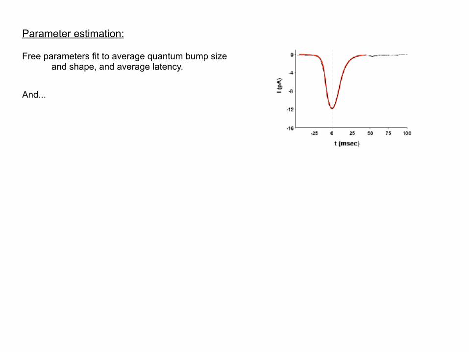
Parameter estimation:
Free parameters fit to average quantum bump size and shape, and average latency.
And...

Parameter estimation:
Free parameters fit to average quantum bump size and shape, and average latency.
And...as you will see soon, the system generates nice looking quantum bumps upon stochastic numerical simulation...

Parameter estimation:
Free parameters fit to average quantum bump size and shape, and average latency.
Results in a “solution manifold”, but basic mechanism of bump generation is independent of specific parameter values.

How can we “see” the system dynamics in some intuitive way? And...what about the stochasticity?

(1) We want to “see” the system dynamics in some intuitive way...and...
(2) System operates at the stochastic limit (1 M*, 1-5 G*, 1-5 PLC*…15-25 B*), so requires stochastic simulation methods (numbers, not concentrations of species).
Let’s deal with item 2 first....the Gillespie method (another interlude).
Pumir et al., PNAS (2008) 105, 10354

Stochastic simulation...the Gillespie method.

Now to deal with stochastic fluctuations…the Gillespie Method
Step 1: The current “state” of the system

Now to deal with stochastic fluctuations…the Gillespie Method
Step 1:
Step 2: Calculate forward and reverse rates for time t
The current “state” of the system

Now to deal with stochastic fluctuations…the Gillespie Method
Step 1:
Step 2:
Step 3:
Calculate forward and reverse rates
The current “state” of the system
Generate two random numbers

Now to deal with stochastic fluctuations…the Gillespie Method
Step 1:
Step 2:
Step 3:
Calculate forward and reverse rates
The current “state” of the system
Generate two random numbers
Update time…so that time steps are a function of how fast the system
dynamics are evolving
Step 4:

Now to deal with stochastic fluctuations…the Gillespie Method
Step 1:
Step 2:
Step 3:
Calculate forward and reverse rates
The current “state” of the system
Generate two random numbers
Update timeStep 4:
Step 5: Update state of system…so that the system statistically moves in
the direction of maximal change
0 1

Now to deal with stochastic fluctuations…the Gillespie Method
Step 1:
Step 2:
Step 3:
Calculate forward and reverse rates
The current “state” of the system
Generate two random numbers
Update timeStep 4:
Step 5: Update state of system
Step 6: Repeat

Stochastic simulation...the Gillespie method.

The result of one trial of Gillespie simulation of this system. “Light stimulation” amounts to creating one active rhodopsin molecule instantly at t=0.
A*
B*
C*

Several quantum bump trials (1M* made at t=0):

How can we “see” the system dynamics in some more intuitive way? This is a seven-dimensional dynamic!!

How can we “see” the system dynamics in some intuitive way? This is a seven-dimensional dynamic!!
But, it turns out that all the reactions except for B* (the channels) and C* (the negative feedback) equilibrate fast. All the relevant dynamics are effectively in a two-dimensional subspace of the overall dynamics!

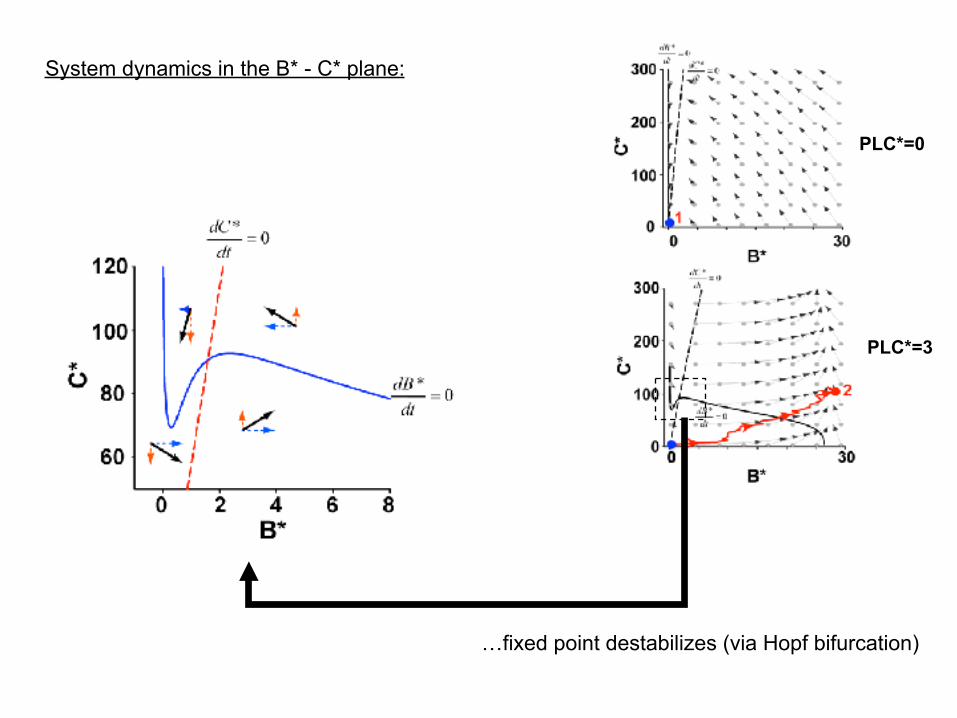
System dynamics in the B* - C* plane:

System dynamics in the B* - C* plane:
PLC*=0

System dynamics in the B* - C* plane:
PLC*=0
…fixed point stable?

System dynamics in the B* - C* plane:
PLC*=0
…a stable fixed point in the dark

System dynamics in the B* - C* plane:
PLC*=0
PLC*=3
System dynamics in the B* - C* plane:
PLC*=0
PLC*=3
…fixed point destabilizes (via Hopf bifurcation)

System dynamics in the B* - C* plane:
PLC*=0
PLC*=3
PLC*=0

System dynamics in the Trp* - B* plane:Again, one trial of stochastic simulation of this system. “Light stimulation” amounts to creating one active rhodopsin molecule instantly at t=0.
C*
B*C
*B
*

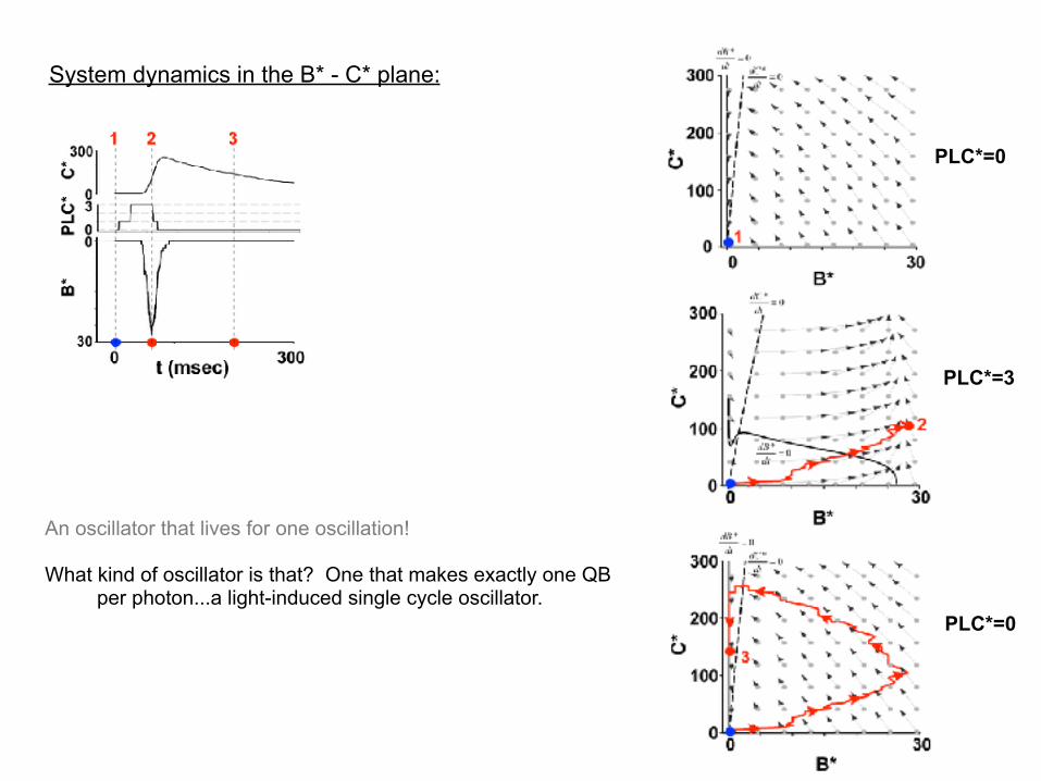
System dynamics in the B* - C* plane:
PLC*=0
PLC*=3
PLC*=0
(1) In the dark, the system has a stable fixed point at B*=0. Per the model, a quantum bump is impossible from thermal activations of Trp channels.

System dynamics in the B* - C* plane:
PLC*=0
PLC*=3
PLC*=0
(1) In the dark, the system has a stable fixed point at B*=0. Per the model, a quantum bump is impossible from thermal activations of Trp channels.
(2) But, upon activation of PLC*, the system dynamics causes the cascade to work as a stochastic relaxation oscillator…building up DAG to where calcium influx through Trp* ignites the positive feedback. This destabilizes the fixed point, triggers a regenerative opening of Trp channels, and causes the system to go through a “limit-cycle oscillation”.
(3) Deactivation of PLC* and build-up of C* shuts-off the bump and causes the system to go into a refractory phase until C* itself deactivates.

System dynamics in the B* - C* plane:
PLC*=0
PLC*=3
PLC*=0
An oscillator that lives for one oscillation!
System dynamics in the B* - C* plane:
PLC*=0
PLC*=3
PLC*=0
An oscillator that lives for one oscillation!
What kind of oscillator is that? One that makes exactly one QB per photon...a light-induced single cycle oscillator.

A test of the model…what if we don’t let M* deactivate?
Computationally…by setting

A test of the prediction of oscillation…what if we don’t let M* deactivate?

A test of the prediction of oscillation…what if we don’t let M* deactivate?
C*
B*
C*
B*
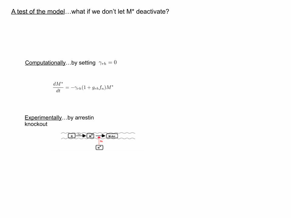
A test of the model…what if we don’t let M* deactivate?
Experimentally…by arrestin knockout
Computationally…by setting

A test of the prediction of oscillation…what if we don’t let M* deactivate?
model w; arr23

So, an explanation for why we get just one bump per photon....
In arrestin knockout
In wild-type

Fundamentally different from the vertebrate rod cell…
D.A. Baylor (1996) PNAS. 93, 560-6
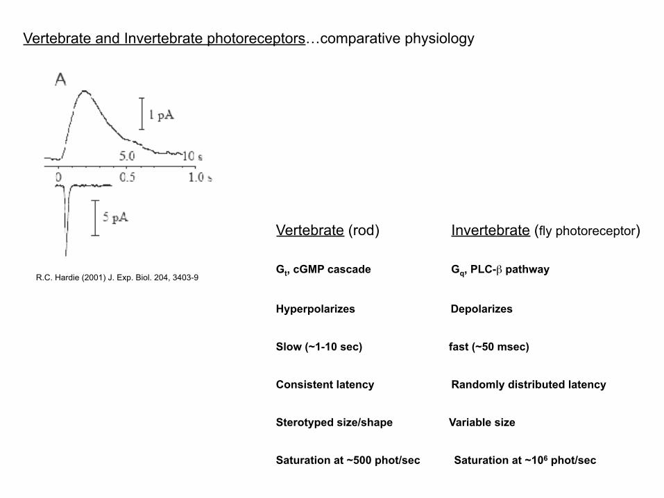
Vertebrate and Invertebrate photoreceptors…comparative physiology
Vertebrate (rod) Invertebrate (fly photoreceptor)
Gt, cGMP cascade Gq, PLC-β pathway
Hyperpolarizes Depolarizes
Slow (~1-10 sec) fast (~50 msec)
Consistent latency Randomly distributed latency
Sterotyped size/shape Variable size
Saturation at ~500 phot/sec Saturation at ~106 phot/sec
R.C. Hardie (2001) J. Exp. Biol. 204, 3403-9

Conclusions
1. The quantum bump is the result of a light-induced non-linear (relaxation) oscillator, converting photons into a fast, all-or-nothing opening of 25-30 ion channels.

Conclusions
1. The quantum bump is the result of a light-induced non-linear (relaxation) oscillator, converting photons into a fast, all-or-nothing opening of 25-30 ion channels.
2. Variable latency comes from the stochasticity of igniting positive feedback and size/shape come from Ca2+-dependent dynamics of positive and negative feedback.
A first explanation of the basic system behaviors....and can drive further experimentation...or...

Conclusions
1. The quantum bump is the result of a light-induced non-linear (relaxation) oscillator, converting photons into a fast, all-or-nothing opening of 25-30 ion channels.
2. Variable latency comes from the stochasticity of igniting positive feedback and size/shape come from Ca2+-dependent dynamics of positive and negative feedback.
3. Single bump per photon is guaranteed by deactivating the relaxation oscillator within one oscillation by shutting off early intermediates in signaling.
4. The reliability of the bump upon photon absorption and the absence of the bump in the dark is explained by the sharp threshold for igniting Ca2+-mediated positive feedback. Below this, vanishingly low bump probability....above this, bumps with probability approaching one.
A first explanation of the basic system behaviors....and can drive further experimentation...or...

Next, we will use everything we have learned up to now to take on the problem of protein function and evolution….a non-linear dynamical system comprised of many parts.
Linear
Nonlinear
n = 1
n = 2 or 3
n >> 1
continuum
exponential growth and decay
single step conformational change
fluorescence emission
pseudo first order kinetics
fixed points
bifurcations, multi stability
irreversible hysteresis
overdamped oscillators
second order reaction kinetics
linear harmonic oscillators
simple feedback control
sequences of conformational change
anharmomic oscillators
relaxation oscillations
predator-prey models
van der Pol systems
Chaotic systems
electrical circuits
molecular dynamics
systems of coupled harmonic oscillators
equilibrium thermodynamics
diffraction, Fourier transforms
systems of non-linear oscillators
non-equilibrium thermodynamics
protein structure/function
neural networks
the cell
ecosystems
Diffusion
Wave propagation
quantum mechanics
viscoelastic systems
Nonlinear wave propagation
Reaction-diffusion in dissipative systems
Turbulent/chaotic flows
adapted from S. Strogatz