lecture 11 - electrical engineering and computer science · eecs 452 { fall 2014 lecture 11 { page...
TRANSCRIPT

Lecture 11Today: Spectrum analysis, windowing
STFT, DFT filterbanksTransfer function measurementInterrupt processing
Announcements: Parts must be ordered by friday.There is a lecture on thursday.No lecture next tuesday (Fall break).Tue lab shifted to Thur next week.Oct 16 practice midterm will be posted.Oct 16 Hwk 5 is due.
References: See last slide.
“Of course the first novel idea was to do the factorization, which you do on penciland paper, put together a program. To get an efficient program you have to have
some way of indexing.”— Jim Cooley talking about how he and Tukey discovered the FFT
Please keep the lab clean and organized. Last one out should close
door!!!!
EECS 452 – Fall 2014 Lecture 11 – Page 1/57 Tue – 10/07/2014

Using DFT/FFT for signal analysis
X[k] =
N−1∑n=0
x[n]e−j2πkn/N , k = 0, 1, . . . , N − 1 .
I The k-th coefficient of the N-point FFT of x[n] is a sample ofthe DTFT of x[n] at digital frequency f = k/N .
I If x[n] are time samples x(nTs) of a continuous time signal x(t)then DTFT is an approximation to the finite time FT of x(t)over the time window t ∈ [0, (N − 1)Ts).
I There are several issues that need to be addressedI Spectral leakageI Spectral resolutionI Time varying spectra
I To build intuition we start by considering an example: DFT ofsinusoidal signal.
EECS 452 – Fall 2014 Lecture 11 – Page 2/57 Tue – 10/07/2014

DFT: sinusoid at on-DFT frequency fc = m/N
DFT of sinusoid x[n] = cos(2πfcn+ φ)?
Assume sinusoidal frequency satisfies fc = m/N for integerm ∈ {0, . . . , N/2} (on-DFT sinusoid)
Use Euler formula: cos(θ) = (ejθ + e−jθ)/2
XDFT (k) =ejφ
2
N−1∑n=0
e−j2πk−mN
n
︸ ︷︷ ︸N∆[k−m]
+e−jφ
2
N−1∑n=0
e−j2πk+mN
n
︸ ︷︷ ︸N∆[N−k−m]
=
{Nejφ
2, k = m
Ne−jφ
2, k = N −m
(∆[n] is kronecker delta function)
EECS 452 – Fall 2014 Lecture 11 – Page 3/57 Tue – 10/07/2014

DFT: sinusoid at off-DFT frequency fc 6= m/N
DFT of sinusoid x[n] = cos(2πfcn+ φ)?
Assume sinusoidal frequency does not satisfy fc = m/N for integerm ∈ {0, . . . , N/2}
XDFT (k) =ejφ
2
N−1∑n=0
e−j2πk−NfcN
n
︸ ︷︷ ︸6=N∆[k−m]
+e−jφ
2
N−1∑n=0
e−j2πk+NfcN
n
︸ ︷︷ ︸6=N∆[N−k−m]
This is the leakage phenomenon and it occurs when fc 6= m/N (off-DFTsinusoid).
EECS 452 – Fall 2014 Lecture 11 – Page 4/57 Tue – 10/07/2014

DFT: sinusoid on-DFT fc = 0.25 = m/N ,
m = 4, N = 64
EECS 452 – Fall 2014 Lecture 11 – Page 5/57 Tue – 10/07/2014

DFT: sinusoid off-DFT fc = 4.5/N
EECS 452 – Fall 2014 Lecture 11 – Page 6/57 Tue – 10/07/2014

DFT: two sinusoids on-DFT fci = mi/N ,
m1 = 4, m2 = 5, N = 64
EECS 452 – Fall 2014 Lecture 11 – Page 7/57 Tue – 10/07/2014

DFT: two sinusoids fci = mi/N ,
m1 = 4(on-DFT), m2 = 4.5(off-DFT), N = 64
EECS 452 – Fall 2014 Lecture 11 – Page 8/57 Tue – 10/07/2014

DFT: two sinusoids on-DFT fci = mi/N ,
m1 = 4, m2 = 5, N = 64
EECS 452 – Fall 2014 Lecture 11 – Page 9/57 Tue – 10/07/2014
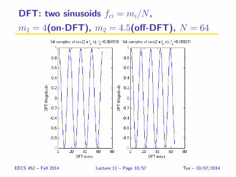
DFT: two sinusoids fci = mi/N ,
m1 = 4(on-DFT), m2 = 4.5(off-DFT), N = 64
EECS 452 – Fall 2014 Lecture 11 – Page 10/57 Tue – 10/07/2014

FFT input scaling
Consider using standard 16-bit Q15 number representation in FFTas in AIC3204.
Let input to the FFT be the cosine signal
cos(2πfcn) =ej2πfcn + e−j2πfcn
2, n = 0, . . . , N − 1
Overflow problem 1: The gain at the fc frequency (assuming itmatches some analysis frequency m/N) is N/2. If a 1024 pointtransform is taken then the result might require 10-1+16 = 25 bits.
Overflow problem 2: A complex input with 16 bit Q15 real andimaginary parts can overflow if a phase rotation occurs. Forexample, 1 + j1 can rotate to 1.414 + j0 creating an overflow in theQ15 real part.
This is why in lab 6 you will be implementing 32 bit precisionFFT’s.
EECS 452 – Fall 2014 Lecture 11 – Page 11/57 Tue – 10/07/2014

An approach to scaling
• Normalization
Consider a Q15 sinewave input having amplitude 1. Using 1/Nscaling on the forward transform, the magnitude of the FFT outputwill be capped at 1/2.
• Distribute normalization over each of the log2(N) layers of FFT
Assume N = 2n is a power of two, n = log2N an integer. Then canapply a scale factor of 1/2 to each layer of the FFT. The net effectwill be to scale the FFT operation by 1/N .
EECS 452 – Fall 2014 Lecture 11 – Page 12/57 Tue – 10/07/2014

Spectral analysis in digital domainDigital spectral analysis of a continuous time signal x(t) ofbandwidth B
I Measure x(t) over a window of time t ∈ [0, T ).
I Sample measured signal at Nyquist rate Fs = 1/Ts = 2B toobtain data record
x[n] = x(nTs), n = 0, . . . , N − 1, N = T/Ts = TFs
I Apply FFT to this data record
X[k] =
N−1∑n=0
x[n]e−j2πkN n, k = 0, . . . , N − 1
I Compute spectrumI Magnitude spectrum |X[k]|I Power spectrum 1
N|X[k]|2
I Phase spectrum argX[k]
EECS 452 – Fall 2014 Lecture 11 – Page 13/57 Tue – 10/07/2014

Example: sinusoid at frequency Fc = fcFs Hz.
x[n] = cos(2πfcn), n = 0, . . . , N − 1
XDTFT (f) =
N−1∑n=0
cos (2πfcn) e−2πfn =1
2
N−1∑n=0
(ej2πfcn + e−j2πfcn
)e−j2πfn
=1
2gN (f − fc) +
1
2gN (f + fc)
gN (ν) =
N−1∑n=0
e−j2πνn
Use geometric series formula∑Mn=0 a
n = (1− aM+1)/(1− a) to obtain
gN (ν) = Ne−jπν(N−1)sin(πνN)
N sin(πν)︸ ︷︷ ︸Dirichlet kernel
EECS 452 – Fall 2014 Lecture 11 – Page 14/57 Tue – 10/07/2014

DTFT of 16 samples of sinusoid: fc = Fc/Fs = k/N
Peaks are at fc, 1− fc. Zeros occur at Fc/Fs ± k/N , k an integer.EECS 452 – Fall 2014 Lecture 11 – Page 15/57 Tue – 10/07/2014

DFT of 16 samples of sinusoid: fc = Fc/Fs = k/N
There is no leakage since fc is equal to k/N for the integer k = 4.EECS 452 – Fall 2014 Lecture 11 – Page 16/57 Tue – 10/07/2014

DTFT of 16 samples of sinusoid: fc = Fc/Fs = 0.27
Peaks occur near fc, 1− fc. There are no zeros in DTFTEECS 452 – Fall 2014 Lecture 11 – Page 17/57 Tue – 10/07/2014

DFT of 16 samples of sinusoid: fc = Fc/Fs = 0.27
There is leakage since fc is not equal to k/N for any integer k.EECS 452 – Fall 2014 Lecture 11 – Page 18/57 Tue – 10/07/2014

DFT spectrum of sum of sinusoids
Q. What can we conclude about the time domain signal x[n] byobserving peaks in |X(k)| at frequencies f = k1/N, . . . , kp/N?
A. Not much unless |X(k)| at all other frequencies is zero.
The reason for the ambiguity on right panel is spectral leakage.
EECS 452 – Fall 2014 Lecture 11 – Page 19/57 Tue – 10/07/2014

DFT spectrum of sum of sinusoids
,
Time domain waveforms in spectra shown on previous slide (N = 64)
x[n] = cos(2πf1n) + 1/2 cos(2πf2n), n = 0, . . . , N − 1
I Left panel: f1 = 4/N , f2 = 5/N . Both analysis frequencies ofN-point DFT.
I Right panel: f1 = 4/N , f2 = 4.5/N . f2 not an analysis frequencyof N-point DFT. |f1− f2| is under DFT’s spectral resolution 1/N .
EECS 452 – Fall 2014 Lecture 11 – Page 20/57 Tue – 10/07/2014

DFT spectrum of sum of sinusoids
,
Illustration of scalloping distortion for two frequencies f1 = 0.1641(= 10.5/N) and f2 = 0.3203 (= 20.5/N). N=64-point FFT.
x[n] = cos(2πf1n) + 1/2 cos(2πf2n), n = 0, . . . , N − 1EECS 452 – Fall 2014 Lecture 11 – Page 21/57 Tue – 10/07/2014
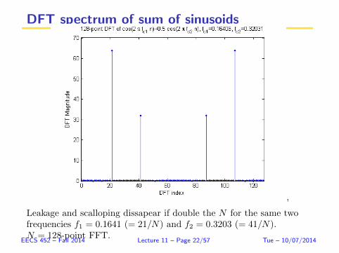
DFT spectrum of sum of sinusoids
,
Leakage and scalloping dissapear if double the N for the same twofrequencies f1 = 0.1641 (= 21/N) and f2 = 0.3203 (= 41/N).N = 128-point FFT.
x[n] = cos(2πf1n) + 1/2 cos(2πf2n), n = 0, . . . , N − 1
EECS 452 – Fall 2014 Lecture 11 – Page 22/57 Tue – 10/07/2014

Resolution vs sensitivity of DFT spectrum
Resolution and sensitivity are the primary ”quality” measures of aspectral analysis method.Frequency resolution: the minimum detectable frequency separationof two sinusoids in the absence of noise.
Frequency resolution is Fs/N = 1/(NTs) = 1/T Hz.
Spectral sensitivity: the minimum amplitude of a sinusoid requiredfor detection against noise background.
Spectral sensitivity depends on several factors
I Nature of background noise
I Number of bits of amplitude resolution (Q(15), Q(31))
I The length of the analysis window T
I Signal-to-noise power ratio (SNR)
EECS 452 – Fall 2014 Lecture 11 – Page 23/57 Tue – 10/07/2014

DFT spectrum with no nse: 10k vs 100k pts
Top: 16384-pt (214) FFT, Bottom 131072-pt (217) FFT
EECS 452 – Fall 2014 Lecture 11 – Page 24/57 Tue – 10/07/2014

DFT spectrum with no nse: 10k vs 100k pts
Top: 16384-pt (214) FFT, Bottom 131072-pt (217) FFT
EECS 452 – Fall 2014 Lecture 11 – Page 25/57 Tue – 10/07/2014

DFT spectrum with 0dB nse: 10k vs 100k pts
Top: 16384-pt (214) FFT, Bottom 131072-pt (217) FFT
EECS 452 – Fall 2014 Lecture 11 – Page 26/57 Tue – 10/07/2014

DFT spectrum with 0dB nse: 10k vs 100k pts
Top: 16384-pt (214) FFT, Bottom 131072-pt (217) FFT
EECS 452 – Fall 2014 Lecture 11 – Page 27/57 Tue – 10/07/2014
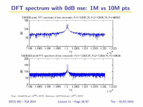
DFT spectrum with 0dB nse: 1M vs 10M pts
Top: 1048576-pt (220) FFT, Bottom 16777216-pt (224) FFT
EECS 452 – Fall 2014 Lecture 11 – Page 28/57 Tue – 10/07/2014

Summarize: DFT spectrum
|XDFT [k]|, k = 0, . . . , N − 1
I DFT index k corresponds to digital frequency fc = k/N and Hzfrequency Fc = Fsk/N .
I Leakage occurs for any frequency component not at one of DFTanalysis frequencies Fsk/N , k = 0, . . . , N/2.
I Frequency resolution of DFT spectrum is Fs/N . This is theminimum frequency separation that can be detected.
I If x(t) is a sum of p sinusoids
x(t) = A1 sin(2πF1t+ φ1) + · · ·+Ap sin(2πFpt+ φp)
Then sinusoids can be detected from DFT spectrum if:I There are no more than p = N/2− 1 sinusoidsI The sinusoidal frequencies Fi are all less than Fs/2 Hz.I The frequency Fc of each sinusoid is distinct and satisfies
Fc/Fs = k/N, k ∈ {0, . . . , N/2}EECS 452 – Fall 2014 Lecture 11 – Page 29/57 Tue – 10/07/2014
How to combat leakage and ambiguity?
Method that is effective: use longer analysis window (increase T )
→ this always reduces leakage for ”long duration” (stationary) signals.
Methods that are not effective for leakage mitigation
I Zero padding, decimating or interpolating the DFT
I Computing the full DTFT
Methods that can be effective
I If frequency estimation is the objective, use a different ”highresolution” spectrum estimator (signal subpace, MUSIC)
I Apply a non-rectangular time window to data prior to DFT(”windowing the data”)
EECS 452 – Fall 2014 Lecture 11 – Page 30/57 Tue – 10/07/2014
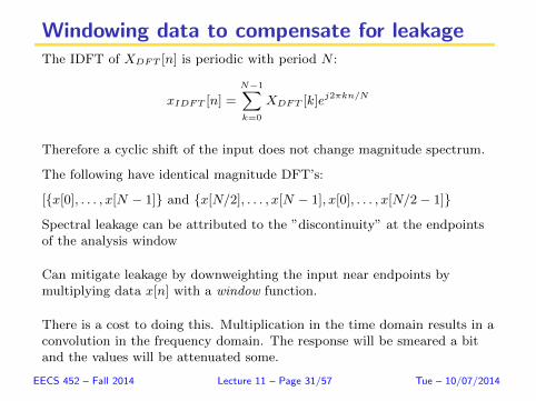
Windowing data to compensate for leakageThe IDFT of XDFT [n] is periodic with period N :
xIDFT [n] =
N−1∑k=0
XDFT [k]ej2πkn/N
Therefore a cyclic shift of the input does not change magnitude spectrum.
The following have identical magnitude DFT’s:
[{x[0], . . . , x[N − 1]} and {x[N/2], . . . , x[N − 1], x[0], . . . , x[N/2− 1]}
Spectral leakage can be attributed to the ”discontinuity” at the endpointsof the analysis window
Can mitigate leakage by downweighting the input near endpoints bymultiplying data x[n] with a window function.
There is a cost to doing this. Multiplication in the time domain results in aconvolution in the frequency domain. The response will be smeared a bitand the values will be attenuated some.
EECS 452 – Fall 2014 Lecture 11 – Page 31/57 Tue – 10/07/2014

Illustration of cyclic discontinuity effect
Plot of samples and therect. window function.
Weighted samples shownre-centered at end pointsplice.
dB plot of the spectrumof the windowed samples.
200 400 600 800 1000−1
−0.5
0
0.5
1
Rectangle (No) Window
−500 0 500−1
−0.5
0
0.5
1
−2 −1.5 −1 −0.5 0 0.5 1 1.5 2
x 104
−80
−60
−40
−20
0dB
Hz
EECS 452 – Fall 2014 Lecture 11 – Page 32/57 Tue – 10/07/2014

Windowing
Select portion of waveform to analyze.
DFT enforces periodicity. . . what happens at the ends?
Weight or shade the data to minimize end effects.
Multiplication in time corresponds to convolution in frequency.
X(k) =
N−1∑n=0
w[n]x[n]e−j2πkn/N , k = 0, 1, . . . , N − 1.
Multiplication in the time domain corresponds to convolution(filtering) in the frequency domain.
EECS 452 – Fall 2014 Lecture 11 – Page 33/57 Tue – 10/07/2014

Many window functions to choose from
EECS 452 – Fall 2014 Lecture 11 – Page 34/57 Tue – 10/07/2014

Window functions used in lab
0 200 400 600 800 10000
0.2
0.4
0.6
0.8
1rectangle
Hamming
Chebyshev
sample index
ampl
itude
Window Functions
EECS 452 – Fall 2014 Lecture 11 – Page 35/57 Tue – 10/07/2014

Rectangular window (no window)
Plot of samples and thewindow function.
Weighted samples shownre-centered at end pointsplice.
dB plot of the spectrumof the windowed samples.
200 400 600 800 1000−1
−0.5
0
0.5
1
Rectangle (No) Window
−500 0 500−1
−0.5
0
0.5
1
−2 −1.5 −1 −0.5 0 0.5 1 1.5 2
x 104
−80
−60
−40
−20
0dB
Hz
EECS 452 – Fall 2014 Lecture 11 – Page 36/57 Tue – 10/07/2014

Hamming window
Plot of samples and thewindow function.
Weighted samples shownre-centered at end pointsplice.
dB plot of the spectrumof the windowed samples.
200 400 600 800 1000−1
−0.5
0
0.5
1
Hamming Window
−500 0 500−1
−0.5
0
0.5
1
−2 −1.5 −1 −0.5 0 0.5 1 1.5 2
x 104
−80
−60
−40
−20
0
dB
Hz
EECS 452 – Fall 2014 Lecture 11 – Page 37/57 Tue – 10/07/2014

Chebyshev 72 dB window
Plot of samples and thewindow function.
Weighted samples shownre-centered at end pointsplice.
dB plot of the spectrumof the windowed samples.
200 400 600 800 1000−1
−0.5
0
0.5
1
Chebyshev 72 dB Window
−500 0 500−1
−0.5
0
0.5
1
−2 −1.5 −1 −0.5 0 0.5 1 1.5 2
x 104
−80
−60
−40
−20
0
dB
Hz
EECS 452 – Fall 2014 Lecture 11 – Page 38/57 Tue – 10/07/2014
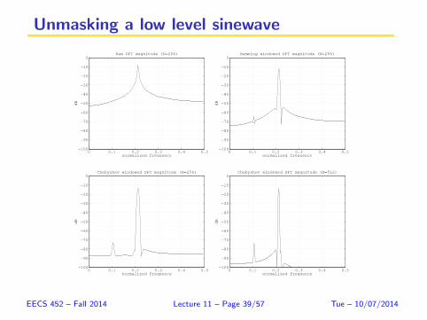
Unmasking a low level sinewave
0 0.1 0.2 0.3 0.4 0.5−100
−90
−80
−70
−60
−50
−40
−30
−20
−10
0Raw DFT magnitude (N=256)
normalized frequency
dB
0 0.1 0.2 0.3 0.4 0.5−100
−90
−80
−70
−60
−50
−40
−30
−20
−10
0Hamming windowed DFT magnitude (N=256)
normalized frequency
dB
0 0.1 0.2 0.3 0.4 0.5−100
−90
−80
−70
−60
−50
−40
−30
−20
−10
0Chebyshev windowed DFT magnitude (N=256)
normalized frequency
dB
0 0.1 0.2 0.3 0.4 0.5−100
−90
−80
−70
−60
−50
−40
−30
−20
−10
0Chebyshev windowed DFT magnitude (N=512)
normalized frequency
dB
EECS 452 – Fall 2014 Lecture 11 – Page 39/57 Tue – 10/07/2014

What are the downsides of windowing?
Main lobe width spreads energy of a frequency component (line) inDTFT. This causes loss of nearby resolution.
Frequency component line amplitudes are reduced.
Scalloping loss causes masking of frequency line that falls midwaybetween adjacent lines.
May need increased numeric precision to implement a windowaccurately.
EECS 452 – Fall 2014 Lecture 11 – Page 40/57 Tue – 10/07/2014

The short time Fourier transform (STFT)
A method for performing time varying spectral analysis with theDFT.
The STFT of a discrete time signal x[n] is defined as
Xm(f) =
∞∑n=−∞
x[n]w[n−mL]e−j2πfm
Where:
I w[n] is a length N window function, e.g., rectangular, hanning,hamming, etc
I L controls the overlap of successive windows for successiveoutput times m (L = N no overlap, L = 1 overlap by N − 1samples).
I f is analysis frequency of interest
Note: X0(f) is ordinary windowed DTFT
EECS 452 – Fall 2014 Lecture 11 – Page 41/57 Tue – 10/07/2014

Short time fourier transform example
http://www.originlab.com/index.aspx?go=Products/OriginPro also see
http://www.ceremade.dauphine.fr/~peyre/numerical-tour/tours/audio_1_processing/.
EECS 452 – Fall 2014 Lecture 11 – Page 42/57 Tue – 10/07/2014

Using DFT as a filter
Define the sliding DFT (identical to STFT for rectangular windowand L = 1)
Xn[k] =
N−1∑m=0
x[n−m]e−j2πfkm, fk = k/N
This produces a time varying DFT that changes over sequentialsamples. For a fixed value of k we can think of the sliding DFT as afilter with input x[n] and output y[n].
y[n] =
∞∑m=∞
hk[m]x[n−m]
where hk[m] = wN (m)e−j2πfkm, wN (m) is rectangular window
{hk[0], . . . , hk[N − 1]} = {1, e−j2πfk , . . . , e−j2πfk(N−1)}
EECS 452 – Fall 2014 Lecture 11 – Page 43/57 Tue – 10/07/2014

Using DFT as a filter
−2 −1.5 −1 −0.5 0 0.5 1 1.5 2
x 104
−80
−60
−40
−20
0
dB
N = 1024, k = 21
DFT as a Filter
0 500 1000 1500 2000−80
−60
−40
−20
0N = 1024, k = 21
dB
Hz
Magnitude transfer function |Hk(f)| of DFT bandpass filter withk = 21 (magnitude of DFT at bin 21 by sweeping input ej2πft
through frequencies from −Fs/2 to Fs/2). Note: no conjugatesymmetry since filter hk[m] is complex valued.
EECS 452 – Fall 2014 Lecture 11 – Page 44/57 Tue – 10/07/2014

The DFT filterbankSliding DFT as a bank of N bandpass filters with passbands atfk = k/N (In figure: ωkT = 2πk/N).
https://ccrma.stanford.edu/~jos/sasp/Filter_Bank_Summation_FBS.html
EECS 452 – Fall 2014 Lecture 11 – Page 45/57 Tue – 10/07/2014
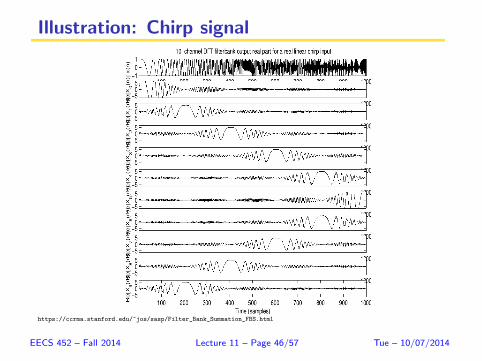
Illustration: Chirp signal
https://ccrma.stanford.edu/~jos/sasp/Filter_Bank_Summation_FBS.html
EECS 452 – Fall 2014 Lecture 11 – Page 46/57 Tue – 10/07/2014

Interrupts
Interrupts are asynchrounous processes (off clock cycle) that arevery common in embedded real time systems.
They are used in the real time implementation of the FFT that youwill implement in Lab 6.
Several steps of interrupt handling
I Enabling: choose the inputs that are allowed to interrupt,keeping track of interrupt priority rankings
I Storing: save the entry state - the system state (data,instruction pointer) when an interrupt occurs.
I Branching: Specify the interrupt service routine (ISR)
I Restoring: restoring the system state to entry state afterinterrupt processing has completed
EECS 452 – Fall 2014 Lecture 11 – Page 47/57 Tue – 10/07/2014
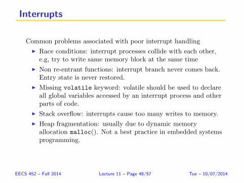
Interrupts
Common problems associated with poor interrupt handling
I Race conditions: interrupt processes collide with each other,e.g, try to write same memory block at the same time
I Non re-entrant functions: interrupt branch never comes back.Entry state is never restored.
I Missing volatile keyword: volatile should be used to declareall global variables accessed by an interrupt process and otherparts of code.
I Stack overflow: interrupts cause too many writes to memory.
I Heap fragmentation: usually due to dynamic memoryallocation malloc(). Not a best practice in embedded systemsprogramming.
EECS 452 – Fall 2014 Lecture 11 – Page 48/57 Tue – 10/07/2014

Transfer function measurement techniquesApply a sinewave at a given frequency to a filter’s input. Measure theoutput’s amplitude and phase. Step the frequency. Repeat. Straightforward but hides any non-linear effects.
Use spectrum analyzer with peak hold capability. Slowly sweep asinewave over the band of interest. Useful for checking for harmonicscaused by nonlinearities. Phase is problematic.
Use white noise input. The the resulting power spectrum is K|H(F )|2.Phase response can also be obtained using cross spectra. Does allfrequencies at once but needs much statistical averaging.
Use wideband PN-sequence, direct or modulating a carrier, to generate abroadband waveform. Transform both filter input and output using aprime factor FFT. Divide input transform into the output transform.This might be covered by US Patent 4,067,060.
First three methods are common in practice and each has it’s place.
EECS 452 – Fall 2014 Lecture 11 – Page 49/57 Tue – 10/07/2014
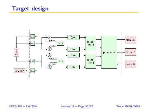
Target design
EECS 452 – Fall 2014 Lecture 11 – Page 50/57 Tue – 10/07/2014

Basics
I Reference cosine/sine waveforms generated by DDS. Only needone DDS.
I In effect, multiplication is by e−j2πFct. Shifts the Fc term to 0Hz. Also shifts −Fc term to −2Fc.
I Sliding average filter has real good null at −2Fc if we integrateover precise number of periods of Fc.
I Convert x and y into polar form.
I Repeat measurements incrementing value of Fc each time tosweep out transfer function, magnitude and phase. Needprovide for filter settling time after each step.
I Display/log/hardcopy.
EECS 452 – Fall 2014 Lecture 11 – Page 51/57 Tue – 10/07/2014
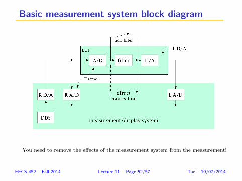
Basic measurement system block diagram
You need to remove the effects of the measurement system from the measurement!
EECS 452 – Fall 2014 Lecture 11 – Page 52/57 Tue – 10/07/2014

Test selection
Simple tests used to check understanding and the ability to act onthat understanding.
I Test 1: A/D to D/A channel check. Right in copied to left out.
I Test 2: Output cosine on right D/A and sine on left D/A.
I Test 3: Left in to filter, filter to left out.
I Else: Filter transfer function measurement.
EECS 452 – Fall 2014 Lecture 11 – Page 53/57 Tue – 10/07/2014

The basic math
Input to filter: A cos(2πFct) = A2
(ej2πFct + e−j2πFct
).
Output of filter:
H(Fc)A cos(2πFct) = A|H(Fc)| cos[2πFct+ θH(Fc)],
=A|H(Fc)|
2
(ej[2πFct+θH(Fc)] + e−j[2πFct+θH(Fc)]
).
Multiply the input and output by e−j(2πFct+θ) and low pass filter:
Input to filter: A2 e−jθ.
Output of filter:A|H(Fc)|
2 ej[θH(Fc)−θ].
EECS 452 – Fall 2014 Lecture 11 – Page 54/57 Tue – 10/07/2014

Recall . . .
Averaging N values is equivalent to filtering the samples.
HA(F ) =e−jπ(N+1)F/Fs
N
sin(πNF/Fs)
sin(πF/Fs).
The gain at F = 0 is 1. The gain at F = −2Fc is∣∣∣∣ sin(πN2Fc/Fs)
sin(π2Fc/Fs)
∣∣∣∣ .This equals 0 for 2πNFc/Fs = kπ where k is an integer. For thesevalues
Fc =kFs2N
.
EECS 452 – Fall 2014 Lecture 11 – Page 55/57 Tue – 10/07/2014

Summary of what we covered today
I Leakage, windowing, spectral estimation
I Interrupts
I Transfer function measurement
EECS 452 – Fall 2014 Lecture 11 – Page 56/57 Tue – 10/07/2014

References
“Applied signal processing,” Dutoit and Marques, 2010.
”Digital signal processing,” Proakis and Manolakis, 3rd Edition.
”Understanding digital signal processing,” R. Lyons, 2004.
”Introduction to interrupt debugging,” Stuart Ball, EE Times5/31/2002http://www.eetimes.com/discussion/beginner-s-corner/4023970/Introduction-to-Interrupt-Debugging
”Five-top-causes-of-nasty-embedded-software-bugs,” Michael Barr,EE Times, 4/1/2010http://eetimes.com/design/embedded/4008917/Five-top-causes-of-nasty-embedded-software-bugs
EECS 452 – Fall 2014 Lecture 11 – Page 57/57 Tue – 10/07/2014