lecture 10 : delaunay triangulation computational geometry prof. dr. th. ottmann 1 overview...

1Lecture 10 :Delaunay Triangulation

Computational GeometryProf. Dr. Th. Ottmann

Overview

• Motivation.

• Triangulation of Planar Point Sets.

• Definition and Characterisitics of the Delaunay Triangulation.

• Computing the Delaunay Triangulation

(randomized, incremental).

• Analysis of Space and Time Requirement.



Motivation

Transformation of a topographic map

into a perspective view



TerrainsGiven: A number of sample points p1..., pn

Required: A triangulation T of the points resulting in a “realistic” terrain.

"Flipping" of an edge:

900

930

2050

900

930

20

50

Goal: Maximise the minimum angle in the triangulation



Triangulation of Planar Point Sets

Given: Set P of n points in the plane (not all collinear).

A triangulation T(P) of P is a planar subdivision of the convex hull of P into triangles with vertices from P.

T(P) is a maximal planar subdivision.

For a given point set there are only finitely many differenttriangulations.



Size of Triangulations

Theorem : Let P be a set of n points in the plane, not all collinear and let k denote the number of points in P that lie on the boundary of convex of hull of P. Then any trianglation of P has 2n-2-k triangles and 3n-3-k edges.

Proof :

Let T be triangulation of P, and let m denote the # of triangles of T. Each triangle has 3 edges, and the unbounded face has k edges. nf = # of faces of triangulation = m + 1 every edge is incident to exactly 2 faces. Hence, # of edges ne = (3m +k)/2. Euler‘s formula : n - ne + nf = 2.Substituting values of ne and nf , we obtain:

m = 2n – 2 – k and ne = 3n – 3 – k .



Angle Vector

Let T(P) be a triangulation of P ( set of n points). Suppose T(P) has m triangles. Consider the 3m angles of triangles of T(P), sorted by increasing value.A(T) = { a1..., a3m } is called angle-vector of T.

Triangulations can be sorted in lexicographical order according to A(T).

A triangulation T(P) is called angle-optimal if A(T(P)) A(T´(P)) for all triangulations T´ of P.



Illegal Edge

a1

a2

a6a5

a3

a4 Pj

Pi a1‘

a2‘ a4‘

a3‘ a5‘

a6‘

Pk

Pj Pi

Edge flip

The edge pi pj is illegal if

6i1min

6i1min

‘i

Note: Let T be a triangulation with an illegal edge e. Let T´ be the triangulation obtained from T by flipping e. Then, A(T´) A(T) .

i



Legal Triangulation

P i

Pk

P j

P l

Definition : A triangulation T(P) is called a legal triangulation, if T(P) does not contain any illegal edges.

Test for illegality

Lemma :

Let edge pipj be incident to triangles pipjpk

and pipjpl , and let C be the circle thru pi,pj and pk . The edge pipj is illegal iff the point pl

lies in the interior of C. Furthermore, if thepoints pi, pj, pk, pl form a convex quadri-lateral and do not lie on a common circle , then exactly one of pipj orpk pl is an illegal edge.



Test of IllegalityObservation:

pl lies inside the circle through pi, pj and pk iff pk lies inside thecircle through pi, pj, pl . When all four points lie on circle, bothpipj and pkpl are legal.



Thales Theorem

a

b

p

q

r

s

pipj

pk

pl

asb aqb = apb arb

illegal

Lemma: Let C be the circle through the triangle pi, pj, pk and let the point pl be the fourth point of a quadrilateral.The edge pipj is illegal iff pl lies in the interior of C.



pi pj

pl

pk

pi pj

pl

pk

Consider the quadrilateral with pl in the interior of the circle that goes through pi, pj, pk.

Claim: The minimum angle does not occur at pk!

(likewise: Minimum angle does not occur at pl )

Goal: Show that pipj is illegal



pi pj

pk

pl

a1a2

a3

a4

pi pj

pk

pl

a1a2

a3

a4

a1‘a2‘

a3‘ a4‘

pi pj

pk

pl

a1‘a2‘

a3‘ a4‘

W.l.o.g.

a4 minimal



pi pj

pk

pl

a1a2

a3

a4

a1‘a2‘

a3‘ a4‘

Circle criterion violated illegal edge



pk

pi

pj

pl

pi

pj

pl

Assumption:edge pkpl is illegal, and circle criterion is not violated

Then: Edge pipj is also illegal,

a contradiction!pk



Circle Criterion

Definition:A triangulation fulfills the circle criterion if and only if the circumcircle of each triangle of the triangulation does not contain any other point in its interior.



Theorems

Theorem:A triangulation T(P) of a set P of points does not contain an illegal edge if and only if nowhere the circle criterion is violated.

Theorem:Every triangulation T(P) of a set P of points can be finally transformed into an angle-optimal triangulation in a finite number of steps.



Definition and characteristics of the Delaunay triangulation

The Delaunay Triangulation DT(G) is the straight line dual of the Voronoi diagram.Vertices: Points (sites) of the Voronoi regions Edges: Between any two points of neighbouring Voronoi regions

Each Voronoi vertex is the center of a triangle of the Delaunay triangulation (for sets of points (sites) in general position).



Planarity of the Delaunay Graph DG(P)

pi

pj

Tij

Cij

Theorem:The Delaunay Triangulation DT(P) of a set of points P is planar.

Proof:Let pipj be an edge of DT(P). Then there is an empty circle Cij, that goes through pi and pj.

Tj, the center of Cij , is on the common edge of V(pi) and V(pj).



t

t contains no sites



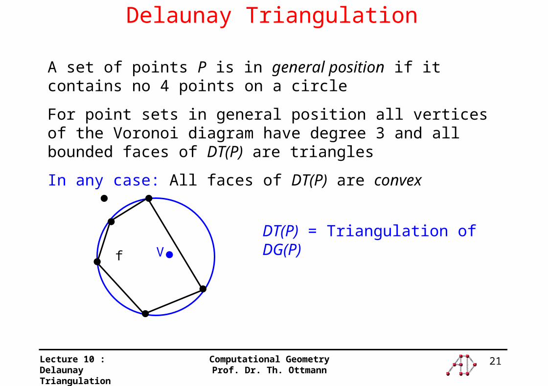
Delaunay Triangulation

Vf

A set of points P is in general position if it contains no 4 points on a circle

For point sets in general position all vertices of the Voronoi diagram have degree 3 and all bounded faces of DT(P) are triangles

In any case: All faces of DT(P) are convex

DT(P) = Triangulation of DG(P)



Characterisation of the Delaunay Triangulation

Theorem:Let P be a set of points in the plane (in general position), and let T be a triangulation of P. Then T is a Delaunay Triangulation of P if and only if the circumcircle of any triangle of T does not contain any other point of P in its interior (i.e. T fulfills the circle criterion).



Equivalent characterisations of the Delaunay Triangulation

1. DT(P) is the straight-line-dual of VD(P).

2. DT(P) is a triangulation of P such that all edges are legal (local angle-optimal).

3. DT(P) is a triangulation of P such that for each triangle the circle criterion is fulfilled.

4. DT(P) is global angle-optimal triangulation.

5. DT(P) is a triangulation of P such that for each edge pipj there is a circle, on which pi and pj lie and which does not contain any other point from P.



Computation of the Delaunay Triangulation (randomized, incremental)

Given: Point set P = {p1..., pn }

Initially: Compute triangle (x, y, z), which includes the points p1..., pn.

m

z (0,3m)

y (3m,0)

x (-3m,-3m)



Algorithm DT(P)

m = max {|xi|,|yi|}

T = ((3m, 0), (3m, 3m), (0, 3m))

1. initialize DT(P) as T.

2. permutate the points in P randomly.

3. for r = 1 to n do

find the triangle in DT(P), which contains pr;

insert new edges in DT(P) to pr;

legalize new edges.

4. remove all edges, which are connected with x, y or z.



Inserting a point

pi

pj

pr

pk

pi

pj

pkpr

pl

pi

pj

pk

pr

2 cases : pr is inside a triangle pr is on an edge

Legalize (pr,pipj,T)if pipj is illegal then Let pipjpk be the triangle adjacent

to prpipj along pipj.Legalize (pr, pipk, T)Legalize (pr, pkpj, T)



Algorithm Delaunay Triangulation Input: A set of points P = {p1..., pn } in general position

Output: The Delaunay triangulation DT(P) of P 1. DT(P) = T = (x, y, z)

2. for r = 1 to n do

3. find a triangle pipjpk T, that contains pr.

4. if pr lies in the interior of the triangle pipjpk

5. then split pipjpk 6. Legalize(pr, pipj), Legalize(pr, pipk),

Legalize(pr, pjpk)

7. if pr lies on an edge of pipjpk (say pipj)

8. then split pipjpk and pipjpl Legalize (pr, pipl), Legalize (pr, pipk), Legalize (pr, pjpl), Legalize (pr, pjpk)

9. Delete (x, y, z) with all incident edges to P



CorrectnessLemma :Every new edge created in the algorithm for constructing DT during the intersection of pr is an edge of the Delaunay graph of

{p1,...,pn} .pq is a Delaunay edge iff there is a (empty) circle, which contains only p and q on the circumference.

Proof idea : Shrink a circle which was empty before addition of pr !



pr

pr

Observation: After insertion of pr , every new edge produced by edge-flips is incident to pr!

Correctness of the algorithm: Consider newly produced edges:



pr

pi

pj

pk

Edge-flips produce only legal edges.

Before inserting pr , circle that goes through pi, pj, pk was empty!

Edge-flips produce edges that are always incident to pr !



Data Structure for Point Location

t1

t2

t3

t2

t3

t4t5

t4

t6

t7

t1 t2

t4 t5

t3

t6 t7

t1 t2 t3

t1 t2 t3

t1 t2

t4 t5

t3

Split t1

flip pipj

flip pipk

pi

pj

pi pk



Analysis of the Algorithm for Constructing DT(P).

Lemma :

The expected number of triangles created by the incremental algorithm for constructing DT(P) is atmost 9n + 1.



Analysis of the Running time

Theorem :

The Delaunay triangulation of a set of P of n points in theplane can be computed in O(n log n) expected time, usingO(n) expected storage.

Proof :

Running time without Point Location :Proportional to the number of created triangles = O(n).

Point Location :The time to locate the point pr in the current triangulationis linear in the number of nodes of D that we visit.

lecture 10 : delaunay triangulation computational geometry prof. dr. th. ottmann 1 overview...

Documents

triangulation tp of

triangles p i p j p

p of n points

triangulation slide

point p

edge p i p j

trianglation of p

faces of triangulation