lecture 1: measuring and understanding poverty lecture 2: poverty...
TRANSCRIPT
Paris School of Economics Lectures March 2009
Lecture 1: Measuring and Understanding PovertyLecture 2: Poverty, Inequality and Growth
Lecture 3: Bailing out the Poorest
Martin RavallionWorld Bank

Paris School of Economics Lectures March 2009
Lecture 1:Measuring and Understanding
Poverty
Martin RavallionWorld Bank

1.1 Poverty lines1.2 Poverty measures1.3 Testing robustness1.4 Decomposing and modeling poverty
TheoryObjective poverty linesSubjective poverty lines
Further reading (this lecture): Martin Ravallion, Poverty Comparisons, Fundamentals of Pure and Applied Economics Volume 56, Harwood Academic Publishers, 1994.

Some theoryThe welfare ratio
• Add up expenditures on all commodities consumed (with imputed values at local market prices) and
• Deflate by a poverty line (depending on household size and composition and location/date)
∑=
==m
ji
i
i
ijiji Z
CZqp
Y1
“real expenditure” or “welfare ratio”
ijp = price paid by household i for good j
ijq = quantity consumed of good j by i
But what is Z?

A poverty line is a money metric of welfare
For informing anti-poverty policies, a poverty line should be absolute in the space of welfare
• This assures that the poverty comparisons are consistent in that two individuals with the same level of welfare are treated the same way.
• As long as the objectives of policy are defined in terms of welfare, and policy choices respect the weak Pareto principle that a welfare gain cannot increase poverty, then welfare consistency in poverty comparisons will be called for.
But what do we mean by “welfare”?

“Welfarist” and capabilities approaches
• Welfarist approach interprets “welfare” as (inter-personally comparable) utility, i.e., attainment of personal satisfaction.– Poverty means not having an income sufficient to attain some
normative (reference) level of utility.• Capabilities approach argues that welfare should be
thought of in terms of the functionings (“beings and doings”) that a person is able to achieve (Amartya Sen)– Poverty means not having an income sufficient to support
specific normative functionings. – Utility can be viewed as one such functioning relevant to well-
being, but only one. – Independently of utility, one might say that a person is better off
if she is able to participate fully in social and economic activity.

Two problems in practiceIdentification problem: how to weight aspects of welfare not
revealed by behavior. • How do family characteristics (such as size and composition) affect
individual welfare at given total household consumption? • How to value command over non-market goods (including some
publicly supplied goods)? • How to measure the individual welfare effect of relative deprivation,
insecurity, social exclusion?
Referencing problem: determining the reference level of welfare above which one is deemed not to be poor — the poverty line in welfare space, which must anchor the money-metric poverty line.
Poverty measurement in practice attempts to expand the information base for addressing the identification and referencing problems

The welfarist approach
The ideal poverty line should then be the minimum cost to a given individual of a reference level of welfare fixed across all individuals
),,( Ziii UXpeZ =
e(.) = expenditure function, giving minimum cost of achieving Uz when facing prices p and with characteristics X.
]),([min)( Ziiiiqi UXqUqpZ ==
Non-welfarist interpretation: reinterpret Uz as a vector of normative functionings.

Linear approximation
∑∑==
=
=⎟⎟⎠
⎞⎜⎜⎝
⎛∂∂=
m
jijij
m
jUUij
iji qppepZ
z
1
*
1
*jq = basic consumption needs (at poverty level of welfare)
i.e., the “poverty basket”
Question: Are there goods that should be included in the consumption aggregate but not the poverty line (“qat” in Yemen) ?

Welfarist interpretation of relative poverty
• Welfare depends on relative income:
(M=mean income)• The poverty line is “absolute” in welfare space, but
“relative” in consumption space.
• Solving gives poverty line as a function of the mean:
• This is the welfarist schedule of relative poverty lines.
)/,( MZZUU z =
)/,( MYYUU =
),( zUMZZ =

The capabilities approach: an interpretation
• Let a person’s functionings be determined by the goods
she consumes and her characteristics.
• Vector of functionings:
),( iii xqff =
Note: • One can postulate that a person derives utility directly
from her functionings. • We can then interpret ),( ii xqu as a derived utility
function, obtained by substituting into the (primal) utility function defined over functionings.
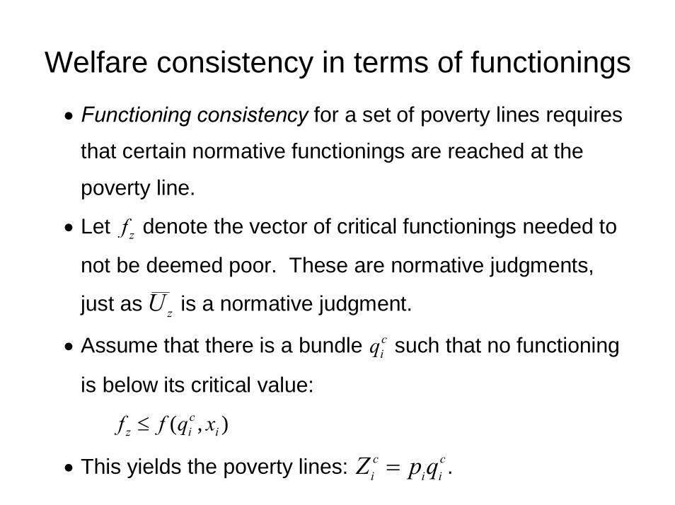
Welfare consistency in terms of functionings• Functioning consistency for a set of poverty lines requires
that certain normative functionings are reached at the
poverty line.
• Let zf denote the vector of critical functionings needed to
not be deemed poor. These are normative judgments,
just as zU is a normative judgment.
• Assume that there is a bundle ciq such that no functioning
is below its critical value:
),( iciz xqff ≤
• This yields the poverty lines: cii
ci qpZ = .

Multiple solutions• There can be multiple solutions for c
iq . • Two ways to pick a unique poverty line can be identified. • Minimum income: Define c
iZ as the minimum income such that ),( i
ciz xqff ≤ holds.
o One (or more) specific functionings will be decisive; that is, the functioning that is the last to reach its critical value as income rises.
o In this sense, the lowest priority functioning for the individual will be decisive.
• Regression method: Treat attainments of the functionings as random variables (that is, with probability distributions) and take a mean conditional on income and other identified covariates.
• Then poverty lines are deemed to be functioning consistent at the income needed to reach zf in expectation.

Regression-based calibration
Imperfect welfare indicator: Wi for household iExamples:• Food share• Nutritional/health status• Self-rated welfare (Cantril scale)• Perceived consumption adequacy
Regression:Wi = a + bYi + cXi + ei (b>0)
Identify normative minima for W, denoted WZ. Then income poverty lines are:
Zi = (WZ - a – cXi)/b

Capabilities interpretation of relative poverty lines
Following Atkinson and Bourguignon we can think of poverty as having both absolute and relative aspects in the income space.
• The former is a failure to attain basic consumption needs, with associated capabilities of being adequately nourished and clothed for meeting the physical needs of survival and normal activities. • On top of this, a person must also satisfy certain social needs, which depend crucially on the prevailing living standards in the place of residence.
Further reading: Anthony Atkinson and Francois Bourguignon, 2001, “Poverty and Inclusion from a World Perspective.” In Joseph Stiglitz and Pierre-Alain Muet (eds) Governance, Equity and Global Markets, Oxford: Oxford University Press.
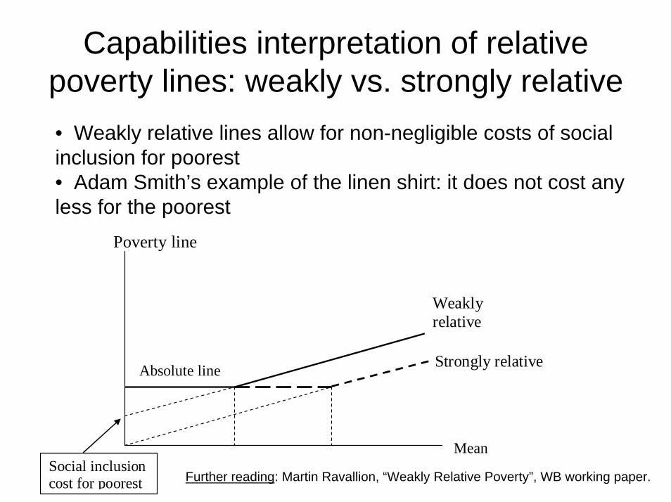
Capabilities interpretation of relative poverty lines: weakly vs. strongly relative
Poverty line
Absolute line
Weakly relative
Strongly relative
Social inclusion cost for poorest
• Weakly relative lines allow for non-negligible costs of social inclusion for poorest• Adam Smith’s example of the linen shirt: it does not cost any less for the poorest
Mean
Further reading: Martin Ravallion, “Weakly Relative Poverty”, WB working paper.

Objective poverty lines in practice
Cost-of-basic-needs methodPoverty line = cost of a bundle of goods deemed sufficient for “basic needs”.
Food-share version:
Cost of food-energy requirementFood-share of “poor”
Food-energy intake method: Find expenditure or income at which food-energy requirements are met on average for each region/socio-economic group
Further reading: Martin Ravallion, Poverty Lines in Theory and Practice, Living Standards Measurement Study Working Paper 133, World Bank, Washington DC., 1998.

Problems in practice
1. Defining "basic consumption needs"• Setting food energy requirements (Variability; multiple equilibria; activity
level).• Setting "basic non-food consumption needs" (behavioral approaches).
2. Consistency in terms of welfare• Is the same standard of living being treated the same way in different sub-
groups of the poverty profile? If not, then the profile may be quite deceptive.
• Is the definition of welfare consistent with the definition of poverty? If some good is purchased by poor people why should it not be included in the poverty bundle?
Key question: how sensitive are the rankings in a poverty profile to these choices?
Further reading: Michael Lokshin and martin Ravallion, “On the Consistency of Poverty Lines”in Poverty, Inequality and Development: Essays in Honor of Erik Thorbecke, edited by Alain de Janvry and Ravi Kanbur, Springer, 2006.

Examples of inconsistent poverty lines
Example 1: “Cost-of-basic-needs method”
% of calories from each source
"urban" rural"
rice 50 40cassava 10 40vegetables 20 10meat 20 10
•The two bundles yield same food-energy intake.• But the "urban" bundle is almost certainly preferable to the "rural" one. • The standard of living at the urban poverty line is higher than at the rural line. • This makes the poverty comparison welfare inconsistent, which can distort policy making based on the poverty profile.

Example 2: "Food-energy intake method"
Different sub-groups attain food energy requirements at different real consumption expenditures. e.g., "rich" urban areas buy more expensive calories than "poor" rural areas.
zu Incom e
Food-energy intake
2100
zr
rural
urban
zu/zr tends to far exceed plausible allowances for differences in cost-of-living
Question: What factors might shift these food-energy consumption functions?Further reading: Martin Ravallion and Benu Bidani, "How Robust is a Poverty Profile?"World Bank Economic Review, Vol. 8, No. 1, January 1994, pp. 75-102.
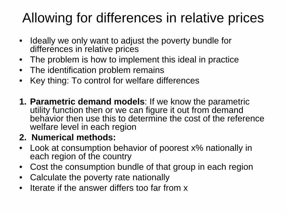
Allowing for differences in relative prices• Ideally we only want to adjust the poverty bundle for
differences in relative prices• The problem is how to implement this ideal in practice• The identification problem remains• Key thing: To control for welfare differences
1. Parametric demand models: If we know the parametric utility function then or we can figure it out from demand behavior then use this to determine the cost of the reference welfare level in each region
2. Numerical methods:• Look at consumption behavior of poorest x% nationally in
each region of the country• Cost the consumption bundle of that group in each region• Calculate the poverty rate nationally• Iterate if the answer differs too far from x

Methods of setting poverty lines do matter!
Head-count index (% poor) Urban Rural Indonesia Food energy method 16.8 14.3 Cost-of-basic needs method
10.7 23.6
Tunisia Food share method 7.3 5.7 Cost-of-basic needs method
3.5 13.1
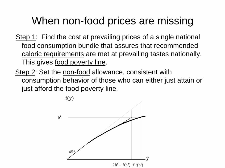
When non-food prices are missingStep 1: Find the cost at prevailing prices of a single national
food consumption bundle that assures that recommended caloric requirements are met at prevailing tastes nationally. This gives food poverty line.
Step 2: Set the non-food allowance, consistent with consumption behavior of those who can either just attain or just afford the food poverty line.
bf
f(y)
yf-1(bf)2bf – f(b f)
45°

Calculating the non-food allowance from an Engel curve
residualXXZYYYf rf +−++= )()/ln(/)( γβαf(Y) = food spending when total spending is Y
= food poverty line
For reference household (in reference region):
Lower poverty line =
Why?• Non-food allowance for lower poverty line is
• But
So upper poverty line = where
fZ
fZ)2( α−
)( ff ZfZ −
α=ff ZZf /)(
*/αfZ )/1log( ** αβαα +=

The Social Subjective Poverty LineThe Minimum Income Question (MIQ)
"What income do you consider to be absolutely minimal, in that you could not make ends meet with any less?“
z* A ctualincom e
Subjective minimumincom e
45°
Is this method suitable for developing countries?
Can one estimate z* without the MIQ?

Subjective poverty lines for developing countries
• Minimum income question is of doubtful relevance to most countries
• Subjective poverty lines can be derived using simple qualitative assessments of consumption adequacy.
• Consumption adequacy question:“Concerning your family’s food consumption over the past one month, which of the following is true?”Less than adequate ...1Just adequate .......…. 2More than adequate.. .3
"Adequate" means no more nor less than what the respondent considers to be the minimum consumption needs of the family.

Modeling consumption adequacy
Individual needs are a latent variable:
Z =βY + πX + ε
Subjective poverty line identified from qualitative data using the model:
Prob(Y > Z) = F[(1-β)Y-α- πX)/σ]
Further reading: Menno Pradhan and Martin Ravallion, “Measuring Poverty Using Qualitative Perceptions of Consumption Adequacy” Review of Economics and Statistics,Vol. 82(3), August 2000, pp. 462-471.

Examples for Jamaica and Nepal
• Respondents asked whether their food, housing and clothing were adequate for their family’s needs. • The implied poverty lines are robust to alternative methods of dealing with other components of expenditure. • The aggregate poverty rates turn out to accord quite closely with those based on independent “objective”poverty lines. • However, there are notable differences in the geographic and demographic poverty profiles.
Poverty lines across countries
• Richer people – and richer countries – tend to have higher poverty lines. – Amongst poor countries, there is very little
income gradient across countries in their poverty lines — absolute consumption needs dominate.
– But the gradient rises as incomes rise. • Also idiosyncratic effects, so we take averages =>
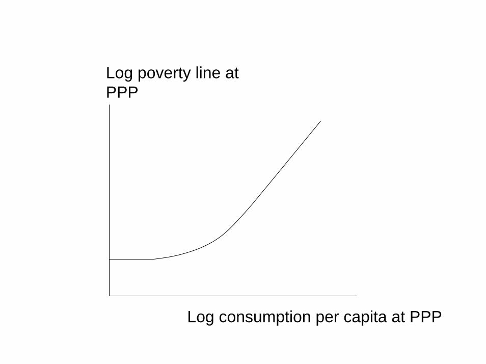
Log poverty line at PPP
Log consumption per capita at PPP

“$1 a day”
• In the 1990 World Development Report, the Bank chose to measure global poverty by the standards of what poverty means in the poorest countries.
• => the “$1/day” line.• Median poverty line of the lowest 10 lines from
original WDR 1990. • => $1.08 at 1993 PPP for consumption.
– Regression based method gives $1.05 (95% CI: $0.88,$1.24) for poorest country.
Further reading: Shaohua Chen and Martin Ravallion, “How Have the World’s Poorest Fared Since the Early 1980s?” World Bank Research Observer, Vol. 19, No.2, Fall 2004, pp. 141-170.

Log poverty line at PPP
$1 a day
Log consumption per capita at PPP

But it is a low poverty line Living at India’s Poverty Line
A person living in rural areas at India’s poverty line in 1993-94 could afford: Consumption/dayGrain (60% rice; 40% wheat) 400 gms Pulses (1/3 masur, 2/3 arhar) 20 gms Milk 70 ml. Eggs 0.2 (no.)
Edible oil (mustard; groundnut) 10 gms Vegetables (potato; onion; brinjal; tomatoes) 120 gms Fresh fruit (bananas; coconut) 0.1 (no.) Dried chili 4 gms Tea leaves 3 gms
After buying this bundle of food items, the person would have left over about Rs.2/day to put toward miscellaneous non-food items. About one third of India’s population cannot afford even this bundle.

0
100
200
300
Nat
iona
l pov
erty
line
($/m
onth
at 2
005
PPP
)
3 4 5 6 7Log consumption per person at 2005 PPP
Note: Fitted values use a lowess smoother with bandwidth=0.8
Latest update: $1.25 a day at 2005 PPPNational poverty lines for developing countries plotted
against mean consumption using consumption PPPs for 2005
OLS elasticity=0.66
$1.25 a day

Strongly vs. weakly relative global lines
]3/,65.0max[$60.0$]3/60.0$,25.1max[$ iii CCZ +=+≡
Poverty line ($ per day; 2005 PPP)
Slope=1/3
$1.25/day
$0.60/day
Weakly relative
Strongly relative
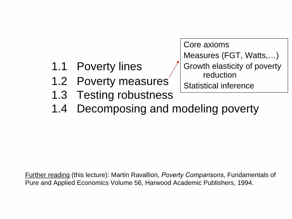
1.1 Poverty lines1.2 Poverty measures1.3 Testing robustness1.4 Decomposing and modeling poverty
Core axiomsMeasures (FGT, Watts,…)Growth elasticity of poverty
reductionStatistical inference
Further reading (this lecture): Martin Ravallion, Poverty Comparisons, Fundamentals of Pure and Applied Economics Volume 56, Harwood Academic Publishers, 1994.

Core axioms1. Focus: A small change in economic welfare for the
non-poor cannot change the measure of poverty2. Monotonicity: A small increase (decrease) in
economic welfare for the poor must reduce (increase) the measure of poverty
3. Sub-group monotonicity: An increase (decrease) in poverty for any sub-group of the population must incraese aggregate measure of poverty.
4. Transfer: A small transfer of income from a poor person to someone who is poorer must decrease the measure of poverty (also called “weak trasnferaxiom”)
1.2 Poverty measures

MeasuresHead-count index
q = no. people deemed poor; n = population size
• Advantage: easily understood• Disadvantages: insensitive to distribution below the
poverty line • The headcount index fails both the Monotonicity and
Transfer Axioms
nqH =
Question: What happens to H if a poor person becomes poorer?

Large gains to the poor but no change in the headcount index

Poverty gap index
∑=
−=
q
i
i
zyz
nPG
1
1
y1,...., yq < z < yq+1, ..., yn
• Advantages of PG: reflects depth of poverty• Disadvantages: insensitive to severity of poverty• Example: A: (1, 2, 3, 4) B: (2, 2, 2, 4)• Let z = 3. HA = 0.75 = HB; PGA = 0.25 = PGB.• The Poverty Gap Index fails the Transfer Axiom
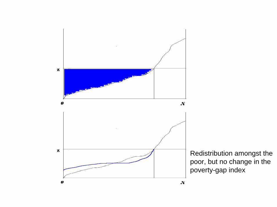
Redistribution amongst the poor, but no change in the poverty-gap index

Interpretation of PG
• The minimum cost of eliminating poverty is (z-µz)q=> perfect targeting. (µz=mean for poor)
• The maximum cost of eliminating poverty: z.n• => No targeting.• Ratio of minimum cost of eliminating poverty to the
maximum cost with no targeting:
• Poverty gap index = potential saving to the poverty alleviation budget from targeting.
Hz
PGz
yznzn
qz zq
i
iz )1(1)(1
µµ−==
−=
−∑=

Squared poverty gap index
∑=
⎟⎠⎞
⎜⎝⎛ −
=q
i
i
zyz
nSPG
1
21
The SPG satisfies all five core axioms
Example: A = (1, 2, 3, 4) B = (2, 2, 2, 4)z = 3 SPGA = 0.14; SPGB = 0.08
Advantage of SPG: sensitive to differences inboth depth and severity of poverty.Disadvantage: difficult to interpret
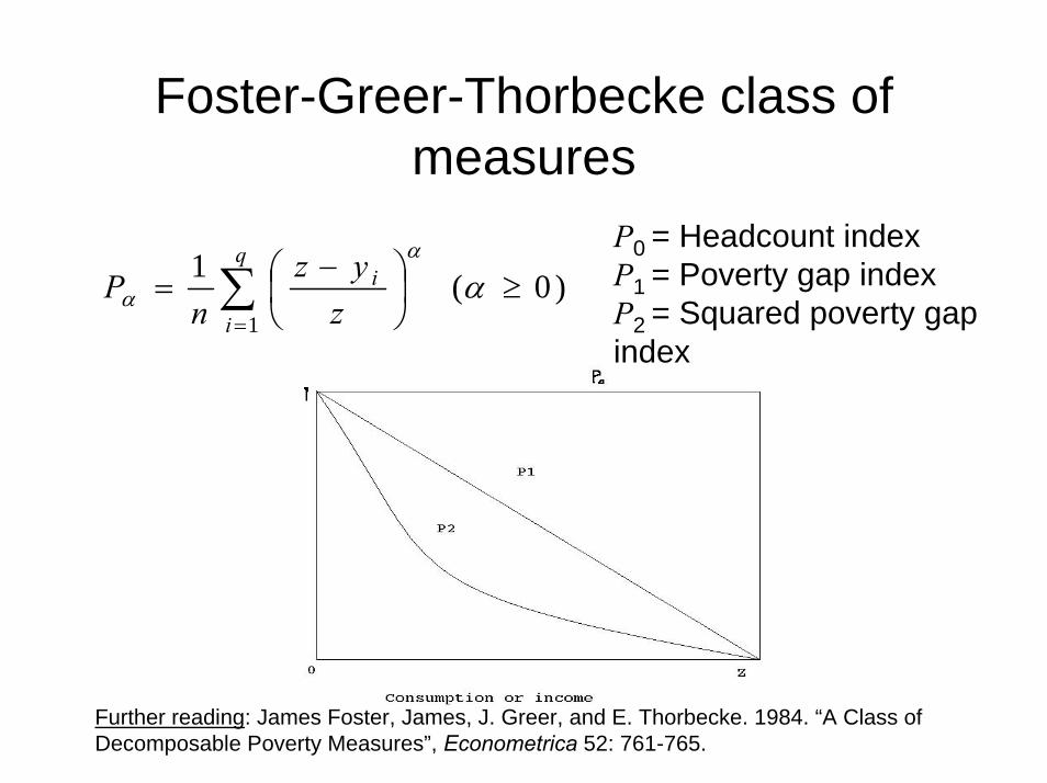
Foster-Greer-Thorbecke class of measures
)0(1
1≥⎟
⎠⎞
⎜⎝⎛ −
= ∑=
αα
α
q
i
i
zyz
nP
P0 = Headcount indexP1 = Poverty gap indexP2 = Squared poverty gapindex
Further reading: James Foster, James, J. Greer, and E. Thorbecke. 1984. “A Class of Decomposable Poverty Measures”, Econometrica 52: 761-765.

The Watts index
(discrete)
(continuous)
• This is the only index satisfying all 17 of the axioms in the poverty measurement literature.
∫
∑
=
==
z
q
ii
W
dxxfxz
yzn
P
0
1
)()/ln(
)/ln(1
Further reading:1. Harold Watts, “An Economic Definition of Poverty,” in D.P. Moynihan (ed.), On Understanding Poverty. New York, Basic Books, 1968. 2. Buhong Zheng, “Axiomatic Characterization of the Watts Index,” Economics Letters 1993, 42, 81-86.

Social welfare and the Watts index
Social welfare:
where
W
z
PdxxfxUdxxfxUW −== ∫∫∞∞
)()()()(0
Further reading:Harold Watts, “An Economic Definition of Poverty,” in D.P. Moynihan (ed.), On Understanding Poverty. New York, Basic Books, 1968.
)/ln()( zxxU =

Mean log censored income
Censored income is . Mean log y* is:
Thus is an exact money metric of the Watts index. Also note that:
Area under the GIC up to the headcount index gives the rate of progress in reducing the Watts index of poverty.
WH
PzzHdppyy −=−+≡ ∫ lnln)1()(lnln0
*
*lny
∫∫ ==−=tt H
t
Ht
Wtt dppgdp
dtpyd
dtdP
dtyd
00
*)()(lnln
Growth Incidence Curve
]),(min[* zpyy ≡

The general class of separable measures
)0),;(;0(),);((0
=<= ∫ αππαπ zzdpzpyP y
H
( )α
π ⎟⎠⎞
⎜⎝⎛ −
=z
pyz )(.FGT:
( ) ⎟⎟⎠
⎞⎜⎜⎝
⎛=
)(ln.
pyzπWatts:
Further reading (including references to other additive measures):Anthony B. Atkinson, “On the Measurement of Poverty,” Econometrica 1987 55: 749-764.
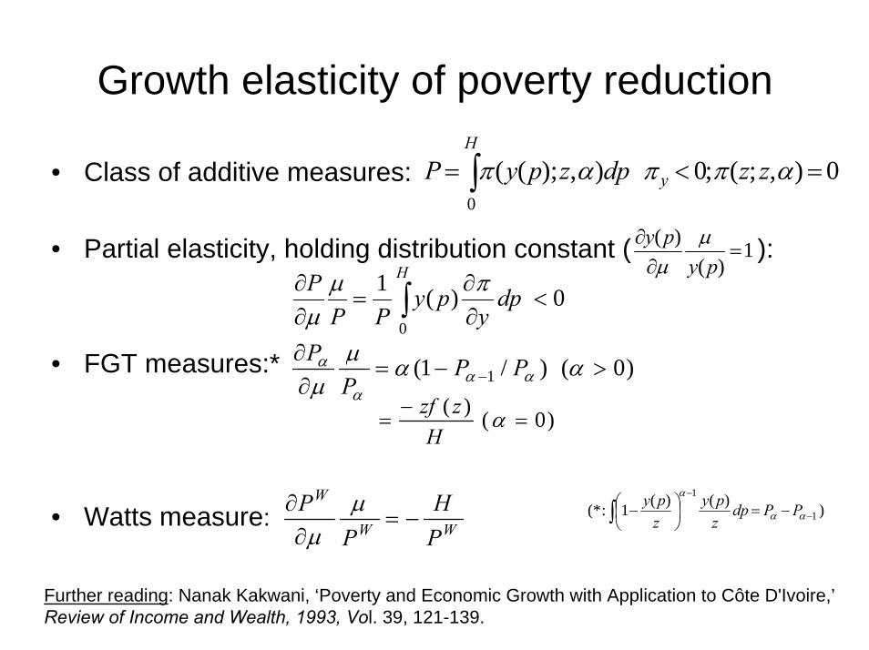
Growth elasticity of poverty reduction
• Class of additive measures:
• Partial elasticity, holding distribution constant ( ):
• FGT measures:*
• Watts measure:
0),;(;0),);((0
=<= ∫ αππαπ zzdpzpyP y
H
0)(1
0
<∂∂
=∂∂
∫H
dpy
pyPP
P πµµ
)0()/1( 1 >−=∂∂
− ααµµ αα
α
α PPP
P
)0()(=
−= α
Hzzf
Further reading: Nanak Kakwani, ‘Poverty and Economic Growth with Application to Côte D'Ivoire,’Review of Income and Wealth, 1993, Vol. 39, 121-139.
1)(
)(=
∂∂
pypy µµ
))()(1:(* 1
1
∫ −
−
−=⎟⎠⎞
⎜⎝⎛ − αα
α
PPdpzpy
zpy
WW
W
PH
PP
−=∂∂ µµ

Statistical inference• Calculating standard errors is easy for additively
separable poverty measures (central limit theorem).Headcount index:
FGT measures:
Watts index:nPPPse /)ˆˆ()( 2
2 ααα −=
nHHHse /)ˆ1(ˆ)( −=
Further reading: Nanak Kakwani, “Statistical Inference in the Measurement of Poverty,” Review of Economics and Statistics, 1993, Vol.75(4): 632-639.
Wq
ii
W Pyzn
Pse ˆ)]/[ln(1)(1
2 −= ∑=
1.1 Poverty lines1.2 Poverty measures1.3 Testing robustness1.4 Decomposing and modeling poverty
Three curvesDominance tests
Further reading (this lecture): Martin Ravallion, Poverty Comparisons, Fundamentals of Pure and Applied Economics Volume 56, Harwood Academic Publishers, 1994.
1.3 Testing robustness1.3 Testing robustnessHow robust are our poverty comparisons to
different measures and lines?
Further reading (section 3.3):• Anthony B. Atkinson, “On the Measurement of Poverty,” Econometrica 1987 55: 749-764.• Martin Ravallion, Poverty Comparisons, Fundamentals of Pure and Applied Economics Volume 56, Harwood Academic Publishers, 1994.
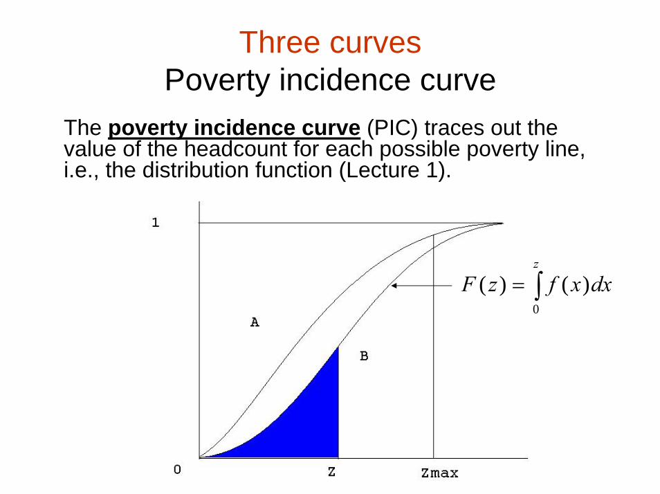
Three curvesPoverty incidence curve
The poverty incidence curve (PIC) traces out the value of the headcount for each possible poverty line, i.e., the distribution function (Lecture 1).
∫=z
dxxfzF0
)()(

Poverty depth curve• The poverty depth curve = area under PIC• Each point on this curve gives aggregate poverty gap –
the poverty gap index times the poverty line z.
∫∫ =−=zz
dxxFdxxfxzzD00
)()()()(

Poverty severity curve• The poverty severity curve = area under poverty
depth curve• Each point gives the squared poverty gap.
∫∫ =−=zz
dxxDdxxFxzzS00
)()()()(

First Order Dominance Test
If the poverty incidence curve for the A distribution is above that for B for all poverty lines up to zmax then there is more poverty in A than B for all poverty measures and all poverty lines up to zmax

What if the poverty incidence curves intersect?
• Ambiguous poverty ranking.• You can either:
i) restrict range of poverty lines ii) restrict class of povertymeasures
Second Order Dominance Test
• If the poverty deficit curve for A is above that for B up to zmax then there is more poverty in A for all poverty measures which are strictly decreasing and weakly convex in consumptions of the poor (e.g. PG and SPG; not H).
• e.g., Higher rice prices in Indonesia: very poor lose, those near the poverty line gain.
• This is equivalent to Generalized Lorenz Dominance (GLC for A lies everywhere below that for B)
What if poverty deficit curves intersect?

Third Order Dominance Test
If the poverty severity curve for A is above that for distribution B then there is more poverty in A, if one restricts attention to distribution sensitive (strictly convex) measures such as SPG.

ExampleInitial State A: (1,2,3) => Final State B: (1.5,1.5,2)
C. F(z) D(z) S(z) A B A B A B 1 1/3 0 1/3 0 1/3 0 1.5 1/3 2/3 2/3 2/3 1 2/3 2 2/3 1 4/3 5/3 7/3 7/3 3 1 1 7/3 8/3 14/3 15/3
Question: What robust conclusions can be drawn about the change in poverty?

Summary of test sequence
• First construct the poverty incidence curves up to highest admissible poverty line for each distribution.
• If they do not intersect, then your comparison is unambiguous.
• If they cross each other then do poverty deficit curvesand restrict range of measures accordingly.
• If they intersect, then do poverty severity curves. • If they intersect then claims about which has more
poverty are contentious.

1.1 Poverty lines1.2 Poverty measures1.3 Testing robustness1.4 Decomposing and modeling poverty
Static modelsDynamics Micro growth models
Further reading (this lecture): Martin Ravallion, Poverty Comparisons, Fundamentals of Pure and Applied Economics Volume 56, Harwood Academic Publishers, 1994.

Static models of poverty
• For all additive measures ("sub-group monotonicity") we can decompose the aggregate measure by sub-groups– e.g., “urban” vs “rural”, “large” vs “small” households
• The poverty profile can be thought of as a simple model of poverty:
Prob(Y < Z)= ∑=
m
jjj DP
1
But this is too simple a model
We would like to introduce a richer set of covariates (some continuous) to:
• Account better for the variance in circumstances leading to poverty
• Disentangle which are the key factors, given their inter-correlation.
For example: • poverty profile shows that rural incidence > urban
incidence, and that poverty is greater for those with least education.
• But education is lower in rural areas. • Is it lack of education or living in rural areas that
increases poverty?

Multivariate poverty profiles
Welfare indicator modeled as a function of multiple variables:
Log(Y/Z) = πX + εor
Log Y = πX + dummy variables for location etc.,+ ε

Probits for poverty
Probit regression for poverty (normally distributed error):
Prob(Y<Z) = Prob(ε < -πX) = F[- πX/σ]
• This is an inefficient way of estimating the OLS regression parameters.• You do not need a probit/logit when the continuous variable is observed.• You can still estimate poverty impacts:
• And under weaker assumptions (e.g., normality of errors is not required)• However, probit may give lower variance predictions of H.
σπ /(.)fXP=
∂∂

Example for VietnamRegression for log household consumption
Coefficient
(t-ratio) Religion: 1 if h'hold head is Buddhist or Christian (0 if other, animist or none) -0.022
(0.82) Ethnic: 1 if h'hold head is of ethnicity other than majority Kinh or Chinese -0.070
(1.65) Locally born: 1 if head is born in the same commune -0.035
(1.29) Age of head 0.007
(1.83) Age² of head -0.059
(1.46) Log household size 0.482
(15.73) Dependency ratio: 1- (ratio of labor age members to all members > 6 yrs old). -0.071
(2.00) Gender of head: male=1 0.008
(0.34) Disabled adult: Labor age adult member is handicapped -0.162
(1.68) Government job: member has worked for gov't in primary/secondary occupation for 5+ yrs, or did so 5 yrs ago or retired from gov't
0.140 (4.83)
SOE job: h’hold member has primary or secondary occupation in State owned enterprise and had it 5 years ago
0.130 (2.74)
Education of head: Household head’s years of education 0.025 (9.48)

Education of other adults: Other h'hold adults’ years of education 0.011 (11.32)
Social Subsidy recipient: dummy var. for receipt of gov't transfers to war heroes, martyrs, disabled etc
0.031 (1.15)
Log allocated irrigated land equivalent 0.131 (7.45)
Private irrigated land 0.028 (2.54)
Private non-irrigated 0.012 (0.98)
Private perennial 0.019 (1.76)
Private water 0.040 (1.50)
Swidden land -0.009 (0.24)
Share of good irrigated 0.042 (1.47)
Share of good non-irrrigated 0.020 (0.81)
Constant 13.47 (68.80)
R² 0.673 F stat Prob>F
92.43 0.0000
N 2810 e: The dependent variable is log household consumption expenditures. Commune fixed effects included. T-ratios in parbased on standard errors corrected for heteroskedasticity and clustering

Studying poverty dynamics using repeated cross-sectional dataDecomposing changes in poverty
Decomposition 1: Growth versus redistribution
Growth component holds relative inequalities (Lorenz curve) constant; redistribution component holds mean constant
Change in poverty between two dates =Change in poverty if distribution had not changed+Change in poverty if the mean had not changed+Interaction effects between growth and redistribution
Growth elasticity of poverty reduction can be used to calculate growth component. However, no reason to assume that the elasticity is constant.

Growth-redistribution decomposition• Let P(µ,L) = poverty measure with mean µ and a vector of
parameters, L, describing the Lorenz curve • The change in poverty between dates 1 and 2 (say) can
then be decomposed as follows:
P2 - P1 = [P(µ2,L1) - P(µ1,L1)] + [P(µ1,L2) - P(µ1,L1)] + residual
growth + redistribution component component
• Growth component = change in poverty attributable to the change in the mean holding the initial Lorenz curve constant.
• Redistribution component = change in poverty attributable to whatever changes in the Lorenz curve occurred, holding the mean constant.
Further reading: Gaurav Datt and Martin Ravallion, "Growth and Redistribution Components of Changes in Poverty", Journal of Development Economics, Vol.38, April 1992, pp. 275-295.

Example for BrazilPoverty and inequality measures
1981 1988 Headcount index (H) (%) 26.5 26.5 Poverty gap index (PG) (x100) 10.1 10.7 Squared poverty gap index (SPG) (x100)
5.0 5.6
Gini index 0.58 0.62
Very little change in poverty; rising inequality
Decomposition Growth
component Redistribution
component Interaction
effect H -4.5 4.5 0.0 PG -2.3 3.2 -0.2 SPG -1.4 2.3 -0.3
• No change in headcount index yet two strong opposing effects: growth (poverty reducing) + redistribution (poverty increasing).• Redistribution effect is dominant for PG and SPG.

Decomposition 2: Gains within sectors vspopulation shifts
• Gains within sectors at given pop. shares;• Population shift effects hold initial poverty measures constant• Interaction effects.

Example: urban-ruraltP = the poverty measure for date t=1,2
itP = the measure for sector i=u,r (urban, rural)
itn = population shares
)])([()]()([ 121112212212uuruuuurrr nnPPPPnPPnPP −−+−+−=−
Within-sector effect Population shift effect
Within-sector effect: the change in poverty weighted by the final year population shares; Population shift effect: the contribution of urbanization, weighted by the initial urban-rural difference in poverty measures. Note: The “population shift effect” should be interpreted as the partial effect of urban-rural migration; it does not allow for any effects of migration and remittances on poverty levels within sectors.

Example for China
Poverty measures (% point change 1981-2001)
H PG SPG
Within rural -32.53 -10.39 -4.51 (72.5) (74.0) (75.0)
Within urban -2.08 -0.32 -0.09 (4.6) (2.3) (1.5)
-10.27 -3.32 -1.42 Population shift (22.9) (23.7) (23.6)
Total change -44.87 -14.04 -6.01
• 75-80% of the drop in national poverty incidence is accountable to poverty reduction within the rural sector; • most of the rest is attributable to urbanization of the population.

Static models on repeated cross-sections
Two time periods, or two sets of householdsAii
Ai XY µπ +=ln for Ai∈
Bii
Bi XY µπ +=ln for Bi∈
How much has the change in poverty been due to:
• Change in the joint distribution of the X’s?• Change in the parameters (“return to the X’s)?
Example 1: in Vietnam, returns to education are significantly higher for the majority ethnic group than minorities
Example 2: in Bangladesh, returns to education are higher in urban areas. Strong geographic effects

Studying poverty dynamics using panel data
Persistently poor:
Poor in both years
Escaped poverty:
Poor in the first period, but not
in second
Poor in first period
Fell into poverty:
Not poor in the first period, but poor in second
Persistently non-poor:
Not poor in either period
Not poor in first period
Poor in second period
Not poor in second period
Panel population
PROT ("Protected") = Change in proportion who fell into poverty.PROM ("Promotion") = Change in proportion escaping poverty.
Further reading: Martin Ravallion, Madhur Gautam and Dominique van de Walle, “Testing a Social Safety Net" Journal of Public Economics, Vol. 57(2), June 1995, pp. 175-199.

Transient vs chronic povertyMeasure of poverty for household i over dates 1,2,…,D:
The transient component of poverty is the part attributed to variability in consumption:
The chronic component is:
iiiDi TCyyP +=),..,( 1
),...,(),...,( 1 iiiDii yyPyyPT −=
),...,( iii yyPC =
Further reading: Martin Ravallion, "Expected Poverty Under Risk Induced Welfare Variability". Economic Journal, Vol. 98, 1988, pp. 1171-1182.

Models of transient and chronic poverty
Transient poverty model
Chronic poverty model
Tii
Ti XT µπ +=
Cii
Ci XC µπ +=
Question: Why might CT ππ ≠ ?

Example for rural ChinaDeterminants of chronic poverty look quite similar (though not
identical) to that for total poverty (chronic plus transient).
However, different determinants of transient poverty• Low foodgrain yields foster chronic poverty, but are not a significant
determinant of transient poverty. • Higher variability over time in physical wealth is associated with
higher transient poverty but lower chronic poverty. • While smaller and better educated households have lower chronic
poverty, these things matter little to transient poverty. • And living in an area with better attainments in health and education
reduces chronic poverty but appears to be irrelevant to transient poverty.
Different models are determining chronic versus transient poverty in rural China.
Further reading: Jyotsna Jalan and Martin Ravallion, “Is Transient Poverty Different? Evidence for Rural China”, Journal of Development Studies, Vol. 36(6), August 2000, pp. 82-99.

Micro growth modelsWith panel data we can also investigate the determinants of why
some households do better than others over time.
• Initial conditions (incl. geographic variables)• Shocks• Policies
Examples of the questions that can be addressed:
• Are there geographic poverty traps?• Does where you live matter independently of individual (non-
geographic) characteristics?• Are there genuine externalities in rural development?• Does this help explain under-development (under-investment in the
externality-generating activities)

Micro growth models cont.,
Micro model of the growth process
Latent heterogeneity in growth process can be dealt with allowing for time varying effects
Quasi-differencing to eliminate the fixed effect
itiitit zxC εξβα +++=∆ ln
(i=1,..,N; t=4,..,T)
ititit µωθε +=
1
11
)1()(ln)1(ln
−
−−
−+−+−+∆+−=∆
ittitit
ittititttit
rzrxrxCrrC
µµξβα
where 1/ −= tttr θθ
As long as 1≠tr we can identify the impacts of the time-invariant observables on the growth process.
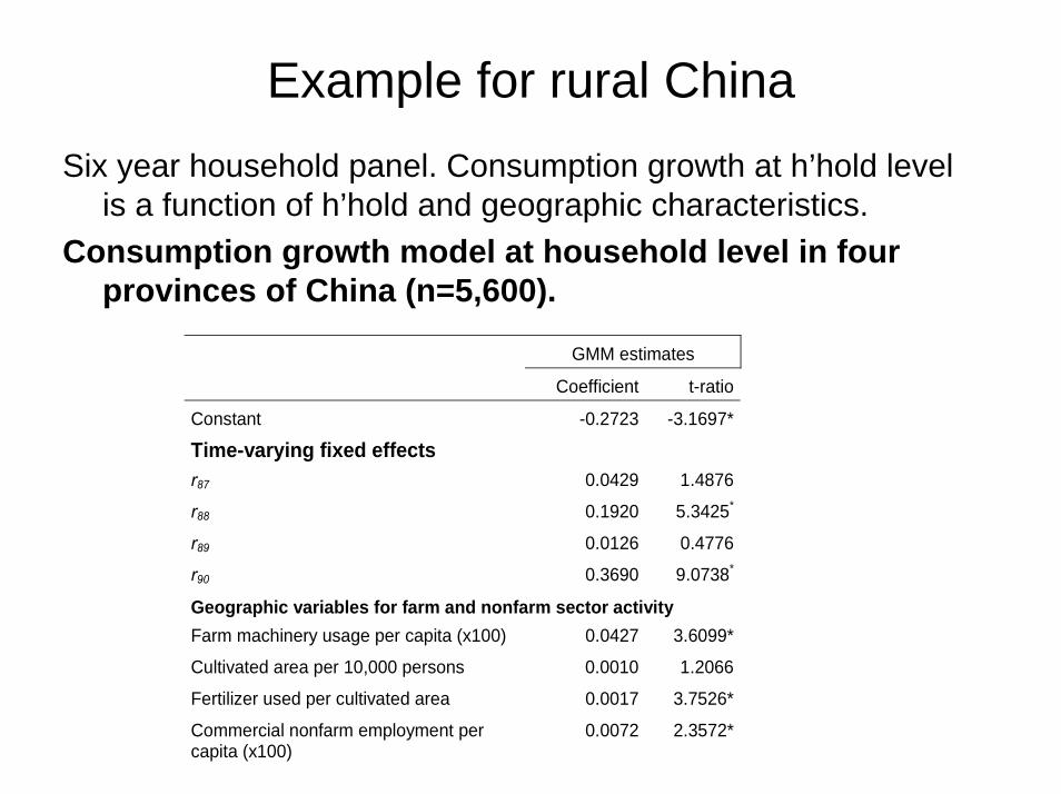
Example for rural ChinaSix year household panel. Consumption growth at h’hold level
is a function of h’hold and geographic characteristics.Consumption growth model at household level in four
provinces of China (n=5,600).
GMM estimates
Coefficient t-ratio
Constant -0.2723 -3.1697*
Time-varying fixed effects r87 0.0429 1.4876
r88 0.1920 5.3425*
r89 0.0126 0.4776
r90 0.3690 9.0738*
Geographic variables for farm and nonfarm sector activity Farm machinery usage per capita (x100) 0.0427 3.6099*
Cultivated area per 10,000 persons 0.0010 1.2066
Fertilizer used per cultivated area 0.0017 3.7526*
Commercial nonfarm employment per capita (x100)
0.0072 2.3572*

Other geographic control variables Guangdong (dummy) 0.0019 0.3688
Guizhou (dummy) 0.0233 4.5430*
Yunnan (dummy) -0.0048 -0.8196
Revolutionary base area (dummy) 0.0207 2.3962*
Border area (dummy) -0.0030 -0.6967
Coastal area (dummy) -0.0099 -1.1877
Minority area (dummy) -0.0037 -1.1051
Mountainous area (dummy) -0.0071 -2.1253*
Plains (dummy) 0.0103 2.7631*
Population density (log) 0.0142 1.5695
Proportion of illiterates in 15+ population (x100)
0.0135 0.7832
Infant mortality rate (x100) -0.0244 -2.0525*
Medical personnel per capita 0.0010 3.5740*
Kilometers of roads per capita (x100) 0.0745 4.4783*
Prop. of population living in the urban areas
-0.0163 -0.7558
Household level variables Expenditure on agricultural inputs per cultivated area (x100)
-0.0866 -4.7395*
Fixed productive assets per capita (x 1000)
0.0037 0.2958
Cultivated land per capita -0.0090 -1.5899
Household size (log) 0.0447 6.9717*

Age of household head 0.0023 2.8483*
Age2 of household head (x 100) -0.0026 -2.9626*
Proportion of adults in the household who are illiterate
0.0087 1.4718
Prop. of adults in the h'hold with primary school education
-0.0028 -0.5816
Prop. of kids in the household between ages 6-11 years
0.0359 3.9065*
Prop. of kids in the h'hold between ages 12-14 years
0.0434 3.3199*
Prop. of kids in the h'hold between ages 15-17 years
0.0075 0.4963
Proportion of kids with primary school education (x 100)
-0.3790 -0.9674
Proportion of kids with secondary school education
0.0193 2.3486*
Whether a household member works in the state sector (dummy)
-0.0101 -1.5062
Proportion of 60+ household members 0.0199 1.6839
Notes: *: indicates significant at 5% level or better.

Findings
• Publicly provided goods, such as rural roads, generate non-negligible gains in consumption relative to the poverty line.
• And since we have allowed for latent geographic effects, the effects of these governmental variables cannot be ascribed to endogenous program placement.
• Aspects of geographic capital relevant to consumption growth embrace both private and publicly provided goods.
• Private investments in agriculture, for example, entail externalbenefits within an area, as do “mixed” goods (involving both private and public provisioning) such as health care.
• Evidence of geographic poverty traps =>

County wealth
Co
un
ty w
ea
lth (
log
)
Household wealth (log)2 4 6 8 10
5
6
7
8
Household wealth
The results strengthen the equity and efficiency case for public investment in lagging poor areas in this setting.
Further reading: Jyotsna Jalan and Martin Ravallion, “Geographic Poverty Traps? A Micro Model of Consumption Growth in Rural China”, Journal of Applied EconometricsVol.17(4), pp. 329-346.