lecture 1: compact kähler manifolds
TRANSCRIPT
Lecture 1: Compact Kahler manifolds
Vincent Guedj
Institut de Mathematiques de Toulouse
PhD course,Rome, April 2021
Vincent Guedj (IMT) Lecture 1: Compact Kahler manifolds April 2021 1 / 19

Quasi-plurisubharmonic functions on Kahler manifolds
The aim of today’s lectures is to
explain the definition and provide examples of Kahler metrics;
motivate the search for canonical Kahler metrics;
discuss basic properties of quasi-plurisubharmonic functions.
The precise plan is as follows:
Lecture 1: a panoramic view of compact Kahler manifolds.
Lecture 2: uniform integrability properties of quasi-psh functions.
Vincent Guedj (IMT) Lecture 1: Compact Kahler manifolds April 2021 2 / 19

Kahler manifolds
Kahler metrics
Let X be a compact complex manifold of dimension n ∈ N∗.
Using localcharts and partition of unity, one can find plenty of hermitian forms,
ωloc=∑n
i ,j=1 ωαβ idzα ∧ dzβ.
where
(zα) are local holomorphic coordinates;
ωαβ are smooth functions such that (ωαβ) is hermitian at all points.
Definition
The hermitian form ω is Kahler if its is closed dω = 0.A manifold is Kahler if it admits a Kahler form.
Euclidean metric in local chart=local example of Kahler metric.
Using cut-off functions destroy the condition dω = 0.
Such a form is associated to a Riemannian metric on TX .
Vincent Guedj (IMT) Lecture 1: Compact Kahler manifolds April 2021 3 / 19

Kahler manifolds
Kahler metrics
Let X be a compact complex manifold of dimension n ∈ N∗. Using localcharts and partition of unity, one can find plenty of hermitian forms,
ωloc=∑n
i ,j=1 ωαβ idzα ∧ dzβ.
where
(zα) are local holomorphic coordinates;
ωαβ are smooth functions such that (ωαβ) is hermitian at all points.
Definition
The hermitian form ω is Kahler if its is closed dω = 0.
A manifold is Kahler if it admits a Kahler form.
Euclidean metric in local chart=local example of Kahler metric.
Using cut-off functions destroy the condition dω = 0.
Such a form is associated to a Riemannian metric on TX .
Vincent Guedj (IMT) Lecture 1: Compact Kahler manifolds April 2021 3 / 19

Kahler manifolds
Kahler metrics
Let X be a compact complex manifold of dimension n ∈ N∗. Using localcharts and partition of unity, one can find plenty of hermitian forms,
ωloc=∑n
i ,j=1 ωαβ idzα ∧ dzβ.
where
(zα) are local holomorphic coordinates;
ωαβ are smooth functions such that (ωαβ) is hermitian at all points.
Definition
The hermitian form ω is Kahler if its is closed dω = 0.A manifold is Kahler if it admits a Kahler form.
Euclidean metric in local chart=local example of Kahler metric.
Using cut-off functions destroy the condition dω = 0.
Such a form is associated to a Riemannian metric on TX .
Vincent Guedj (IMT) Lecture 1: Compact Kahler manifolds April 2021 3 / 19

Kahler manifolds
Kahler metrics
Let X be a compact complex manifold of dimension n ∈ N∗. Using localcharts and partition of unity, one can find plenty of hermitian forms,
ωloc=∑n
i ,j=1 ωαβ idzα ∧ dzβ.
where
(zα) are local holomorphic coordinates;
ωαβ are smooth functions such that (ωαβ) is hermitian at all points.
Definition
The hermitian form ω is Kahler if its is closed dω = 0.A manifold is Kahler if it admits a Kahler form.
Euclidean metric in local chart=local example of Kahler metric.
Using cut-off functions destroy the condition dω = 0.
Such a form is associated to a Riemannian metric on TX .
Vincent Guedj (IMT) Lecture 1: Compact Kahler manifolds April 2021 3 / 19

Kahler manifolds
Examples
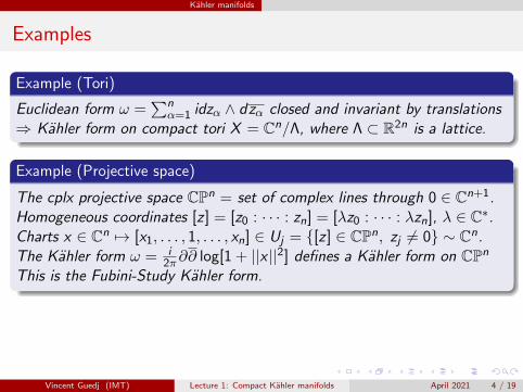
Example (Tori)
Euclidean form ω =∑n
α=1 idzα ∧ dzα closed
and invariant by translations⇒ Kahler form on compact tori X = Cn/Λ, where Λ ⊂ R2n is a lattice.
Example (Projective space)
The cplx projective space CPn = set of complex lines through 0 ∈ Cn+1.Homogeneous coordinates [z ] = [z0 : · · · : zn] = [λz0 : · · · : λzn], λ ∈ C∗.Charts x ∈ Cn 7→ [x1, . . . , 1, . . . , xn] ∈ Uj = {[z ] ∈ CPn, zj 6= 0} ∼ Cn.The Kahler form ω = i
2π∂∂ log[1 + ||x ||2] defines a Kahler form on CPn
This is the Fubini-Study Kahler form. Exercise: check that∫CPn ω
n = 1.
Example (Hopf surface)
The surface X = C2/〈z 7→ 2z〉 ∼ S1×S3 does not admit any Kahler form.
Vincent Guedj (IMT) Lecture 1: Compact Kahler manifolds April 2021 4 / 19

Kahler manifolds
Examples
Example (Tori)
Euclidean form ω =∑n
α=1 idzα ∧ dzα closed and invariant by translations
⇒ Kahler form on compact tori X = Cn/Λ, where Λ ⊂ R2n is a lattice.
Example (Projective space)
The cplx projective space CPn = set of complex lines through 0 ∈ Cn+1.Homogeneous coordinates [z ] = [z0 : · · · : zn] = [λz0 : · · · : λzn], λ ∈ C∗.Charts x ∈ Cn 7→ [x1, . . . , 1, . . . , xn] ∈ Uj = {[z ] ∈ CPn, zj 6= 0} ∼ Cn.The Kahler form ω = i
2π∂∂ log[1 + ||x ||2] defines a Kahler form on CPn
This is the Fubini-Study Kahler form. Exercise: check that∫CPn ω
n = 1.
Example (Hopf surface)
The surface X = C2/〈z 7→ 2z〉 ∼ S1×S3 does not admit any Kahler form.
Vincent Guedj (IMT) Lecture 1: Compact Kahler manifolds April 2021 4 / 19

Kahler manifolds
Examples
Example (Tori)
Euclidean form ω =∑n
α=1 idzα ∧ dzα closed and invariant by translations⇒ Kahler form on compact tori X = Cn/Λ, where Λ ⊂ R2n is a lattice.
Example (Projective space)
The cplx projective space CPn = set of complex lines through 0 ∈ Cn+1.
Homogeneous coordinates [z ] = [z0 : · · · : zn] = [λz0 : · · · : λzn], λ ∈ C∗.Charts x ∈ Cn 7→ [x1, . . . , 1, . . . , xn] ∈ Uj = {[z ] ∈ CPn, zj 6= 0} ∼ Cn.The Kahler form ω = i
2π∂∂ log[1 + ||x ||2] defines a Kahler form on CPn
This is the Fubini-Study Kahler form. Exercise: check that∫CPn ω
n = 1.
Example (Hopf surface)
The surface X = C2/〈z 7→ 2z〉 ∼ S1×S3 does not admit any Kahler form.
Vincent Guedj (IMT) Lecture 1: Compact Kahler manifolds April 2021 4 / 19

Kahler manifolds
Examples
Example (Tori)
Euclidean form ω =∑n
α=1 idzα ∧ dzα closed and invariant by translations⇒ Kahler form on compact tori X = Cn/Λ, where Λ ⊂ R2n is a lattice.
Example (Projective space)
The cplx projective space CPn = set of complex lines through 0 ∈ Cn+1.Homogeneous coordinates [z ] = [z0 : · · · : zn] = [λz0 : · · · : λzn], λ ∈ C∗.
Charts x ∈ Cn 7→ [x1, . . . , 1, . . . , xn] ∈ Uj = {[z ] ∈ CPn, zj 6= 0} ∼ Cn.The Kahler form ω = i
2π∂∂ log[1 + ||x ||2] defines a Kahler form on CPn
This is the Fubini-Study Kahler form. Exercise: check that∫CPn ω
n = 1.
Example (Hopf surface)
The surface X = C2/〈z 7→ 2z〉 ∼ S1×S3 does not admit any Kahler form.
Vincent Guedj (IMT) Lecture 1: Compact Kahler manifolds April 2021 4 / 19

Kahler manifolds
Examples
Example (Tori)
Euclidean form ω =∑n
α=1 idzα ∧ dzα closed and invariant by translations⇒ Kahler form on compact tori X = Cn/Λ, where Λ ⊂ R2n is a lattice.
Example (Projective space)
The cplx projective space CPn = set of complex lines through 0 ∈ Cn+1.Homogeneous coordinates [z ] = [z0 : · · · : zn] = [λz0 : · · · : λzn], λ ∈ C∗.Charts x ∈ Cn 7→ [x1, . . . , 1, . . . , xn] ∈ Uj = {[z ] ∈ CPn, zj 6= 0} ∼ Cn.
The Kahler form ω = i2π∂∂ log[1 + ||x ||2] defines a Kahler form on CPn
This is the Fubini-Study Kahler form. Exercise: check that∫CPn ω
n = 1.
Example (Hopf surface)
The surface X = C2/〈z 7→ 2z〉 ∼ S1×S3 does not admit any Kahler form.
Vincent Guedj (IMT) Lecture 1: Compact Kahler manifolds April 2021 4 / 19

Kahler manifolds
Examples
Example (Tori)
Euclidean form ω =∑n
α=1 idzα ∧ dzα closed and invariant by translations⇒ Kahler form on compact tori X = Cn/Λ, where Λ ⊂ R2n is a lattice.
Example (Projective space)
The cplx projective space CPn = set of complex lines through 0 ∈ Cn+1.Homogeneous coordinates [z ] = [z0 : · · · : zn] = [λz0 : · · · : λzn], λ ∈ C∗.Charts x ∈ Cn 7→ [x1, . . . , 1, . . . , xn] ∈ Uj = {[z ] ∈ CPn, zj 6= 0} ∼ Cn.The Kahler form ω = i
2π∂∂ log[1 + ||x ||2] defines a Kahler form on CPn
This is the Fubini-Study Kahler form. Exercise: check that∫CPn ω
n = 1.
Example (Hopf surface)
The surface X = C2/〈z 7→ 2z〉 ∼ S1×S3 does not admit any Kahler form.
Vincent Guedj (IMT) Lecture 1: Compact Kahler manifolds April 2021 4 / 19
Kahler manifolds
Examples
Example (Tori)
Euclidean form ω =∑n
α=1 idzα ∧ dzα closed and invariant by translations⇒ Kahler form on compact tori X = Cn/Λ, where Λ ⊂ R2n is a lattice.
Example (Projective space)
The cplx projective space CPn = set of complex lines through 0 ∈ Cn+1.Homogeneous coordinates [z ] = [z0 : · · · : zn] = [λz0 : · · · : λzn], λ ∈ C∗.Charts x ∈ Cn 7→ [x1, . . . , 1, . . . , xn] ∈ Uj = {[z ] ∈ CPn, zj 6= 0} ∼ Cn.The Kahler form ω = i
2π∂∂ log[1 + ||x ||2] defines a Kahler form on CPn
This is the Fubini-Study Kahler form.
Exercise: check that∫CPn ω
n = 1.
Example (Hopf surface)
The surface X = C2/〈z 7→ 2z〉 ∼ S1×S3 does not admit any Kahler form.
Vincent Guedj (IMT) Lecture 1: Compact Kahler manifolds April 2021 4 / 19

Kahler manifolds
Examples
Example (Tori)
Euclidean form ω =∑n
α=1 idzα ∧ dzα closed and invariant by translations⇒ Kahler form on compact tori X = Cn/Λ, where Λ ⊂ R2n is a lattice.
Example (Projective space)
The cplx projective space CPn = set of complex lines through 0 ∈ Cn+1.Homogeneous coordinates [z ] = [z0 : · · · : zn] = [λz0 : · · · : λzn], λ ∈ C∗.Charts x ∈ Cn 7→ [x1, . . . , 1, . . . , xn] ∈ Uj = {[z ] ∈ CPn, zj 6= 0} ∼ Cn.The Kahler form ω = i
2π∂∂ log[1 + ||x ||2] defines a Kahler form on CPn
This is the Fubini-Study Kahler form. Exercise: check that∫CPn ω
n = 1.
Example (Hopf surface)
The surface X = C2/〈z 7→ 2z〉 ∼ S1×S3 does not admit any Kahler form.
Vincent Guedj (IMT) Lecture 1: Compact Kahler manifolds April 2021 4 / 19

Kahler manifolds
Basic constructions
If ω is Kahler, then so is ω + i∂∂ϕ if ϕ ∈ C∞(X ,R) is C2-small.
A product of compact Kahler manifolds is Kahler, cfω(x , y) = ω1(x) + ω2(y) = Kahler form on X × Y .
If f : X → Y is a holomorphic embedding and ωY Kahler, thenωX = f ∗ωY is a Kahler form on X .
⇒ a submanifold of a compact Kahler manifold is Kahler.
⇒ any projective algebraic manifold is Kahler.
⇒ any compact Riemann surface is Kahler.
Vincent Guedj (IMT) Lecture 1: Compact Kahler manifolds April 2021 5 / 19

Kahler manifolds
Basic constructions
If ω is Kahler, then so is ω + i∂∂ϕ if ϕ ∈ C∞(X ,R) is C2-small.
A product of compact Kahler manifolds is Kahler,
cfω(x , y) = ω1(x) + ω2(y) = Kahler form on X × Y .
If f : X → Y is a holomorphic embedding and ωY Kahler, thenωX = f ∗ωY is a Kahler form on X .
⇒ a submanifold of a compact Kahler manifold is Kahler.
⇒ any projective algebraic manifold is Kahler.
⇒ any compact Riemann surface is Kahler.
Vincent Guedj (IMT) Lecture 1: Compact Kahler manifolds April 2021 5 / 19

Kahler manifolds
Basic constructions
If ω is Kahler, then so is ω + i∂∂ϕ if ϕ ∈ C∞(X ,R) is C2-small.
A product of compact Kahler manifolds is Kahler, cfω(x , y) = ω1(x) + ω2(y) = Kahler form on X × Y .
If f : X → Y is a holomorphic embedding and ωY Kahler, thenωX = f ∗ωY is a Kahler form on X .
⇒ a submanifold of a compact Kahler manifold is Kahler.
⇒ any projective algebraic manifold is Kahler.
⇒ any compact Riemann surface is Kahler.
Vincent Guedj (IMT) Lecture 1: Compact Kahler manifolds April 2021 5 / 19

Kahler manifolds
Basic constructions
If ω is Kahler, then so is ω + i∂∂ϕ if ϕ ∈ C∞(X ,R) is C2-small.
A product of compact Kahler manifolds is Kahler, cfω(x , y) = ω1(x) + ω2(y) = Kahler form on X × Y .
If f : X → Y is a holomorphic embedding and ωY Kahler,
thenωX = f ∗ωY is a Kahler form on X .
⇒ a submanifold of a compact Kahler manifold is Kahler.
⇒ any projective algebraic manifold is Kahler.
⇒ any compact Riemann surface is Kahler.
Vincent Guedj (IMT) Lecture 1: Compact Kahler manifolds April 2021 5 / 19

Kahler manifolds
Basic constructions
If ω is Kahler, then so is ω + i∂∂ϕ if ϕ ∈ C∞(X ,R) is C2-small.
A product of compact Kahler manifolds is Kahler, cfω(x , y) = ω1(x) + ω2(y) = Kahler form on X × Y .
If f : X → Y is a holomorphic embedding and ωY Kahler, thenωX = f ∗ωY is a Kahler form on X .
⇒ a submanifold of a compact Kahler manifold is Kahler.
⇒ any projective algebraic manifold is Kahler.
⇒ any compact Riemann surface is Kahler.
Vincent Guedj (IMT) Lecture 1: Compact Kahler manifolds April 2021 5 / 19

Kahler manifolds
Basic constructions
If ω is Kahler, then so is ω + i∂∂ϕ if ϕ ∈ C∞(X ,R) is C2-small.
A product of compact Kahler manifolds is Kahler, cfω(x , y) = ω1(x) + ω2(y) = Kahler form on X × Y .
If f : X → Y is a holomorphic embedding and ωY Kahler, thenωX = f ∗ωY is a Kahler form on X .
⇒ a submanifold of a compact Kahler manifold is Kahler.
⇒ any projective algebraic manifold is Kahler.
⇒ any compact Riemann surface is Kahler.
Vincent Guedj (IMT) Lecture 1: Compact Kahler manifolds April 2021 5 / 19

Kahler manifolds
Blow-ups
Example (Local blow up of a point)
Let B be a ball centered at zero in Cn
and consider
B = {(z , `) ∈ B × Pn−1, z ∈ `}.
This is a complex manifold of Cn × Pn−1 of dimension n such that
the projection π : (z , `) ∈ B 7→ z ∈ B satisfies E := π−1(0) ∼ Pn−1;
π is a biholomorphism from B \ E onto B \ {0};ω = π∗ddc(log |z |+ |z |2)− [E ] is a Kahler form on B
Can globalize this construction, blowing up an arbitrary point in X .
One can also blow up any submanifold Y ⊂ X of codimension ≥ 2.
The blow up of a Kahler manifold is a Kahler manifold.
Vincent Guedj (IMT) Lecture 1: Compact Kahler manifolds April 2021 6 / 19

Kahler manifolds
Blow-ups
Example (Local blow up of a point)
Let B be a ball centered at zero in Cn and consider
B = {(z , `) ∈ B × Pn−1, z ∈ `}.
This is a complex manifold of Cn × Pn−1 of dimension n such that
the projection π : (z , `) ∈ B 7→ z ∈ B satisfies E := π−1(0) ∼ Pn−1;
π is a biholomorphism from B \ E onto B \ {0};
ω = π∗ddc(log |z |+ |z |2)− [E ] is a Kahler form on B
Can globalize this construction, blowing up an arbitrary point in X .
One can also blow up any submanifold Y ⊂ X of codimension ≥ 2.
The blow up of a Kahler manifold is a Kahler manifold.
Vincent Guedj (IMT) Lecture 1: Compact Kahler manifolds April 2021 6 / 19

Kahler manifolds
Blow-ups
Example (Local blow up of a point)
Let B be a ball centered at zero in Cn and consider
B = {(z , `) ∈ B × Pn−1, z ∈ `}.
This is a complex manifold of Cn × Pn−1 of dimension n such that
the projection π : (z , `) ∈ B 7→ z ∈ B satisfies E := π−1(0) ∼ Pn−1;
π is a biholomorphism from B \ E onto B \ {0};ω = π∗ddc(log |z |+ |z |2)− [E ] is a Kahler form on B
Can globalize this construction, blowing up an arbitrary point in X .
One can also blow up any submanifold Y ⊂ X of codimension ≥ 2.
The blow up of a Kahler manifold is a Kahler manifold.
Vincent Guedj (IMT) Lecture 1: Compact Kahler manifolds April 2021 6 / 19

Kahler manifolds
Blow-ups
Example (Local blow up of a point)
Let B be a ball centered at zero in Cn and consider
B = {(z , `) ∈ B × Pn−1, z ∈ `}.
This is a complex manifold of Cn × Pn−1 of dimension n such that
the projection π : (z , `) ∈ B 7→ z ∈ B satisfies E := π−1(0) ∼ Pn−1;
π is a biholomorphism from B \ E onto B \ {0};ω = π∗ddc(log |z |+ |z |2)− [E ] is a Kahler form on B
Can globalize this construction, blowing up an arbitrary point in X .
One can also blow up any submanifold Y ⊂ X of codimension ≥ 2.
The blow up of a Kahler manifold is a Kahler manifold.
Vincent Guedj (IMT) Lecture 1: Compact Kahler manifolds April 2021 6 / 19

Kahler manifolds
Local characterizations
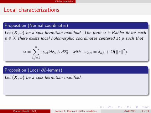
Proposition (Normal coordinates)
Let (X , ω) be a cplx hermitian manifold.
The form ω is Kahler iff for eachp ∈ X there exists local holomorphic coordinates centered at p such that
ω =n∑
i ,j=1
ωαβ idzα ∧ dzβ with ωαβ = δαβ + O(||z ||2).
Proposition (Local ∂∂-lemma)
Let (X , ω) be a cplx hermitian manifold. The form ω is Kahler iff locally
ω = i∂∂ϕ,
where ϕ is smooth and strictly plurisubharmonic.
↪→ Not usually possible globally (max principle), but...
Vincent Guedj (IMT) Lecture 1: Compact Kahler manifolds April 2021 7 / 19

Kahler manifolds
Local characterizations
Proposition (Normal coordinates)
Let (X , ω) be a cplx hermitian manifold. The form ω is Kahler iff for eachp ∈ X
there exists local holomorphic coordinates centered at p such that
ω =n∑
i ,j=1
ωαβ idzα ∧ dzβ with ωαβ = δαβ + O(||z ||2).
Proposition (Local ∂∂-lemma)
Let (X , ω) be a cplx hermitian manifold. The form ω is Kahler iff locally
ω = i∂∂ϕ,
where ϕ is smooth and strictly plurisubharmonic.
↪→ Not usually possible globally (max principle), but...
Vincent Guedj (IMT) Lecture 1: Compact Kahler manifolds April 2021 7 / 19

Kahler manifolds
Local characterizations
Proposition (Normal coordinates)
Let (X , ω) be a cplx hermitian manifold. The form ω is Kahler iff for eachp ∈ X there exists local holomorphic coordinates centered at p such that
ω =n∑
i ,j=1
ωαβ idzα ∧ dzβ with ωαβ = δαβ + O(||z ||2).
Proposition (Local ∂∂-lemma)
Let (X , ω) be a cplx hermitian manifold. The form ω is Kahler iff locally
ω = i∂∂ϕ,
where ϕ is smooth and strictly plurisubharmonic.
↪→ Not usually possible globally (max principle), but...
Vincent Guedj (IMT) Lecture 1: Compact Kahler manifolds April 2021 7 / 19
Kahler manifolds
Local characterizations
Proposition (Normal coordinates)
Let (X , ω) be a cplx hermitian manifold. The form ω is Kahler iff for eachp ∈ X there exists local holomorphic coordinates centered at p such that
ω =n∑
i ,j=1
ωαβ idzα ∧ dzβ with ωαβ = δαβ + O(||z ||2).
Proposition (Local ∂∂-lemma)
Let (X , ω) be a cplx hermitian manifold.
The form ω is Kahler iff locally
ω = i∂∂ϕ,
where ϕ is smooth and strictly plurisubharmonic.
↪→ Not usually possible globally (max principle), but...
Vincent Guedj (IMT) Lecture 1: Compact Kahler manifolds April 2021 7 / 19

Kahler manifolds
Local characterizations
Proposition (Normal coordinates)
Let (X , ω) be a cplx hermitian manifold. The form ω is Kahler iff for eachp ∈ X there exists local holomorphic coordinates centered at p such that
ω =n∑
i ,j=1
ωαβ idzα ∧ dzβ with ωαβ = δαβ + O(||z ||2).
Proposition (Local ∂∂-lemma)
Let (X , ω) be a cplx hermitian manifold. The form ω is Kahler iff locally
ω = i∂∂ϕ,
where ϕ is smooth and strictly plurisubharmonic.
↪→ Not usually possible globally (max principle), but...
Vincent Guedj (IMT) Lecture 1: Compact Kahler manifolds April 2021 7 / 19

Kahler manifolds
The (global) ∂∂-lemma
A Kahler form ω defines a deRham class {ω} ∈ H2(X ,R).
Theorem (∂∂-lemma)
If two Kahler forms ω, ω′ define the same cohomology class, then thereexists a (essentially unique) ϕ ∈ C∞(X ,R) such that ω′ = ω + i∂∂ϕ.
Let Kω denote set of smooth functions ϕ s.t. ω+ i∂∂ϕ > 0 is Kahler.
PSH(X , ω) =the closure of Kω in L1 will be the hero of Lecture 2.
Theorem (Hodge decomposition theorem)
If X is compact Kahler then Hp,q(X ,C) is isomorphic to Hq,p(X ,C) and
Hk(X ,C) = ⊕p+q=kHp,q(X ,C).
↪→ In particular b1(X ) = 2h1,0(X ) even, while b1(S1×S3) = 1 so no Hopf.
Vincent Guedj (IMT) Lecture 1: Compact Kahler manifolds April 2021 8 / 19

Kahler manifolds
The (global) ∂∂-lemma
A Kahler form ω defines a deRham class {ω} ∈ H2(X ,R).
Theorem (∂∂-lemma)
If two Kahler forms ω, ω′ define the same cohomology class,
then thereexists a (essentially unique) ϕ ∈ C∞(X ,R) such that ω′ = ω + i∂∂ϕ.
Let Kω denote set of smooth functions ϕ s.t. ω+ i∂∂ϕ > 0 is Kahler.
PSH(X , ω) =the closure of Kω in L1 will be the hero of Lecture 2.
Theorem (Hodge decomposition theorem)
If X is compact Kahler then Hp,q(X ,C) is isomorphic to Hq,p(X ,C) and
Hk(X ,C) = ⊕p+q=kHp,q(X ,C).
↪→ In particular b1(X ) = 2h1,0(X ) even, while b1(S1×S3) = 1 so no Hopf.
Vincent Guedj (IMT) Lecture 1: Compact Kahler manifolds April 2021 8 / 19

Kahler manifolds
The (global) ∂∂-lemma
A Kahler form ω defines a deRham class {ω} ∈ H2(X ,R).
Theorem (∂∂-lemma)
If two Kahler forms ω, ω′ define the same cohomology class, then thereexists a (essentially unique) ϕ ∈ C∞(X ,R) such that ω′ = ω + i∂∂ϕ.
Let Kω denote set of smooth functions ϕ s.t. ω+ i∂∂ϕ > 0 is Kahler.
PSH(X , ω) =the closure of Kω in L1 will be the hero of Lecture 2.
Theorem (Hodge decomposition theorem)
If X is compact Kahler then Hp,q(X ,C) is isomorphic to Hq,p(X ,C) and
Hk(X ,C) = ⊕p+q=kHp,q(X ,C).
↪→ In particular b1(X ) = 2h1,0(X ) even, while b1(S1×S3) = 1 so no Hopf.
Vincent Guedj (IMT) Lecture 1: Compact Kahler manifolds April 2021 8 / 19

Kahler manifolds
The (global) ∂∂-lemma
A Kahler form ω defines a deRham class {ω} ∈ H2(X ,R).
Theorem (∂∂-lemma)
If two Kahler forms ω, ω′ define the same cohomology class, then thereexists a (essentially unique) ϕ ∈ C∞(X ,R) such that ω′ = ω + i∂∂ϕ.
Let Kω denote set of smooth functions ϕ s.t. ω+ i∂∂ϕ > 0 is Kahler.
PSH(X , ω) =the closure of Kω in L1 will be the hero of Lecture 2.
Theorem (Hodge decomposition theorem)
If X is compact Kahler then Hp,q(X ,C) is isomorphic to Hq,p(X ,C)
and
Hk(X ,C) = ⊕p+q=kHp,q(X ,C).
↪→ In particular b1(X ) = 2h1,0(X ) even, while b1(S1×S3) = 1 so no Hopf.
Vincent Guedj (IMT) Lecture 1: Compact Kahler manifolds April 2021 8 / 19

Kahler manifolds
The (global) ∂∂-lemma
A Kahler form ω defines a deRham class {ω} ∈ H2(X ,R).
Theorem (∂∂-lemma)
If two Kahler forms ω, ω′ define the same cohomology class, then thereexists a (essentially unique) ϕ ∈ C∞(X ,R) such that ω′ = ω + i∂∂ϕ.
Let Kω denote set of smooth functions ϕ s.t. ω+ i∂∂ϕ > 0 is Kahler.
PSH(X , ω) =the closure of Kω in L1 will be the hero of Lecture 2.
Theorem (Hodge decomposition theorem)
If X is compact Kahler then Hp,q(X ,C) is isomorphic to Hq,p(X ,C) and
Hk(X ,C) = ⊕p+q=kHp,q(X ,C).
↪→ In particular b1(X ) = 2h1,0(X ) even, while b1(S1×S3) = 1 so no Hopf.
Vincent Guedj (IMT) Lecture 1: Compact Kahler manifolds April 2021 8 / 19

Kahler manifolds
The (global) ∂∂-lemma
A Kahler form ω defines a deRham class {ω} ∈ H2(X ,R).
Theorem (∂∂-lemma)
If two Kahler forms ω, ω′ define the same cohomology class, then thereexists a (essentially unique) ϕ ∈ C∞(X ,R) such that ω′ = ω + i∂∂ϕ.
Let Kω denote set of smooth functions ϕ s.t. ω+ i∂∂ϕ > 0 is Kahler.
PSH(X , ω) =the closure of Kω in L1 will be the hero of Lecture 2.
Theorem (Hodge decomposition theorem)
If X is compact Kahler then Hp,q(X ,C) is isomorphic to Hq,p(X ,C) and
Hk(X ,C) = ⊕p+q=kHp,q(X ,C).
↪→ In particular b1(X ) = 2h1,0(X ) even,
while b1(S1×S3) = 1 so no Hopf.
Vincent Guedj (IMT) Lecture 1: Compact Kahler manifolds April 2021 8 / 19

Kahler manifolds
The (global) ∂∂-lemma
A Kahler form ω defines a deRham class {ω} ∈ H2(X ,R).
Theorem (∂∂-lemma)
If two Kahler forms ω, ω′ define the same cohomology class, then thereexists a (essentially unique) ϕ ∈ C∞(X ,R) such that ω′ = ω + i∂∂ϕ.
Let Kω denote set of smooth functions ϕ s.t. ω+ i∂∂ϕ > 0 is Kahler.
PSH(X , ω) =the closure of Kω in L1 will be the hero of Lecture 2.
Theorem (Hodge decomposition theorem)
If X is compact Kahler then Hp,q(X ,C) is isomorphic to Hq,p(X ,C) and
Hk(X ,C) = ⊕p+q=kHp,q(X ,C).
↪→ In particular b1(X ) = 2h1,0(X ) even, while b1(S1×S3) = 1 so no Hopf.
Vincent Guedj (IMT) Lecture 1: Compact Kahler manifolds April 2021 8 / 19

Projective manifolds
Holomorphic line bundle
Definition
A holomorphic line bundle Lπ→ X is a complex manifold s.t.
for each x ∈ X , Lx = π−1(x) ∼ C is a complex line,
the projection map π : L→ X is holomorphic,
for each x ∈ X , there exists an open neighborhood U ⊂ X of x and
ϕU : π−1(U)→ U × Ca biholomorphism taking Lx isomorphically onto {x} × C.
Maps ϕU ◦ ϕ−1V induce an automorphisme of U ∩ V × C of the form
ϕU ◦ ϕ−1V : (x , ζ) ∈ U ∩ V × C 7→ (x , gUV (x) · ζ) ∈ U ∩ V × C
where gUV =non vanishing holomorphic functions. Can consider
tensor products L1 ⊗ L2 with transition functions g1UV · g2
UV .L∗ dual line bundle with dual fibers L∗x , st L⊗ L∗ =trivial line bundle.
↪→ Picard group. In the sequel Lj := L⊗ · · · ⊗ L (j times).
Vincent Guedj (IMT) Lecture 1: Compact Kahler manifolds April 2021 9 / 19

Projective manifolds
Holomorphic line bundle
Definition
A holomorphic line bundle Lπ→ X is a complex manifold s.t.
for each x ∈ X , Lx = π−1(x) ∼ C is a complex line,
the projection map π : L→ X is holomorphic,
for each x ∈ X , there exists an open neighborhood U ⊂ X of x and
ϕU : π−1(U)→ U × Ca biholomorphism taking Lx isomorphically onto {x} × C.
Maps ϕU ◦ ϕ−1V induce an automorphisme of U ∩ V × C of the form
ϕU ◦ ϕ−1V : (x , ζ) ∈ U ∩ V × C 7→ (x , gUV (x) · ζ) ∈ U ∩ V × C
where gUV =non vanishing holomorphic functions.
Can consider
tensor products L1 ⊗ L2 with transition functions g1UV · g2
UV .L∗ dual line bundle with dual fibers L∗x , st L⊗ L∗ =trivial line bundle.
↪→ Picard group. In the sequel Lj := L⊗ · · · ⊗ L (j times).
Vincent Guedj (IMT) Lecture 1: Compact Kahler manifolds April 2021 9 / 19

Projective manifolds
Holomorphic line bundle
Definition
A holomorphic line bundle Lπ→ X is a complex manifold s.t.
for each x ∈ X , Lx = π−1(x) ∼ C is a complex line,
the projection map π : L→ X is holomorphic,
for each x ∈ X , there exists an open neighborhood U ⊂ X of x and
ϕU : π−1(U)→ U × Ca biholomorphism taking Lx isomorphically onto {x} × C.
Maps ϕU ◦ ϕ−1V induce an automorphisme of U ∩ V × C of the form
ϕU ◦ ϕ−1V : (x , ζ) ∈ U ∩ V × C 7→ (x , gUV (x) · ζ) ∈ U ∩ V × C
where gUV =non vanishing holomorphic functions. Can consider
tensor products L1 ⊗ L2 with transition functions g1UV · g2
UV .
L∗ dual line bundle with dual fibers L∗x , st L⊗ L∗ =trivial line bundle.
↪→ Picard group. In the sequel Lj := L⊗ · · · ⊗ L (j times).
Vincent Guedj (IMT) Lecture 1: Compact Kahler manifolds April 2021 9 / 19

Projective manifolds
Holomorphic line bundle
Definition
A holomorphic line bundle Lπ→ X is a complex manifold s.t.
for each x ∈ X , Lx = π−1(x) ∼ C is a complex line,
the projection map π : L→ X is holomorphic,
for each x ∈ X , there exists an open neighborhood U ⊂ X of x and
ϕU : π−1(U)→ U × Ca biholomorphism taking Lx isomorphically onto {x} × C.
Maps ϕU ◦ ϕ−1V induce an automorphisme of U ∩ V × C of the form
ϕU ◦ ϕ−1V : (x , ζ) ∈ U ∩ V × C 7→ (x , gUV (x) · ζ) ∈ U ∩ V × C
where gUV =non vanishing holomorphic functions. Can consider
tensor products L1 ⊗ L2 with transition functions g1UV · g2
UV .L∗ dual line bundle with dual fibers L∗x , st L⊗ L∗ =trivial line bundle.
↪→ Picard group. In the sequel Lj := L⊗ · · · ⊗ L (j times).
Vincent Guedj (IMT) Lecture 1: Compact Kahler manifolds April 2021 9 / 19

Projective manifolds
Holomorphic line bundle
Definition
A holomorphic line bundle Lπ→ X is a complex manifold s.t.
for each x ∈ X , Lx = π−1(x) ∼ C is a complex line,
the projection map π : L→ X is holomorphic,
for each x ∈ X , there exists an open neighborhood U ⊂ X of x and
ϕU : π−1(U)→ U × Ca biholomorphism taking Lx isomorphically onto {x} × C.
Maps ϕU ◦ ϕ−1V induce an automorphisme of U ∩ V × C of the form
ϕU ◦ ϕ−1V : (x , ζ) ∈ U ∩ V × C 7→ (x , gUV (x) · ζ) ∈ U ∩ V × C
where gUV =non vanishing holomorphic functions. Can consider
tensor products L1 ⊗ L2 with transition functions g1UV · g2
UV .L∗ dual line bundle with dual fibers L∗x , st L⊗ L∗ =trivial line bundle.
↪→ Picard group. In the sequel Lj := L⊗ · · · ⊗ L (j times).Vincent Guedj (IMT) Lecture 1: Compact Kahler manifolds April 2021 9 / 19

Projective manifolds
Holomorphic sections
Definition
A holomorphic section of L is a holomorphic map s : X → L s.t. π ◦ s = Id.
We let H0(X , L) denote the set of (global) holomorphic sections.
In practice s = {sU} collection of holom maps satisfying sV = gUV sU .
Can add two holomorphic sections and multiply by a complex number.
If s0, . . . , sN is a basis of H0(X , L)=vector space, can consider
x ∈ X 7−→ φL(x) = [s0(x) : · · · : sN(x)] ∈ CPN
Definition
A holomorphic line bundle L is called very ample if φL is an embedding.L is called ample if φLk is very ample for some k >> 1.
Vincent Guedj (IMT) Lecture 1: Compact Kahler manifolds April 2021 10 / 19

Projective manifolds
Holomorphic sections
Definition
A holomorphic section of L is a holomorphic map s : X → L s.t. π ◦ s = Id.We let H0(X , L) denote the set of (global) holomorphic sections.
In practice s = {sU} collection of holom maps satisfying sV = gUV sU .
Can add two holomorphic sections and multiply by a complex number.
If s0, . . . , sN is a basis of H0(X , L)=vector space, can consider
x ∈ X 7−→ φL(x) = [s0(x) : · · · : sN(x)] ∈ CPN
Definition
A holomorphic line bundle L is called very ample if φL is an embedding.L is called ample if φLk is very ample for some k >> 1.
Vincent Guedj (IMT) Lecture 1: Compact Kahler manifolds April 2021 10 / 19

Projective manifolds
Holomorphic sections
Definition
A holomorphic section of L is a holomorphic map s : X → L s.t. π ◦ s = Id.We let H0(X , L) denote the set of (global) holomorphic sections.
In practice s = {sU} collection of holom maps satisfying sV = gUV sU .
Can add two holomorphic sections and multiply by a complex number.
If s0, . . . , sN is a basis of H0(X , L)=vector space, can consider
x ∈ X 7−→ φL(x) = [s0(x) : · · · : sN(x)] ∈ CPN
Definition
A holomorphic line bundle L is called very ample if φL is an embedding.
L is called ample if φLk is very ample for some k >> 1.
Vincent Guedj (IMT) Lecture 1: Compact Kahler manifolds April 2021 10 / 19

Projective manifolds
Holomorphic sections
Definition
A holomorphic section of L is a holomorphic map s : X → L s.t. π ◦ s = Id.We let H0(X , L) denote the set of (global) holomorphic sections.
In practice s = {sU} collection of holom maps satisfying sV = gUV sU .
Can add two holomorphic sections and multiply by a complex number.
If s0, . . . , sN is a basis of H0(X , L)=vector space, can consider
x ∈ X 7−→ φL(x) = [s0(x) : · · · : sN(x)] ∈ CPN
Definition
A holomorphic line bundle L is called very ample if φL is an embedding.L is called ample if φLk is very ample for some k >> 1.
Vincent Guedj (IMT) Lecture 1: Compact Kahler manifolds April 2021 10 / 19

Projective manifolds
Example: the hyperplane bundle
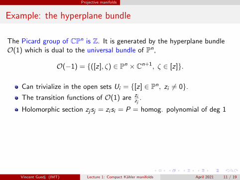
The Picard group of CPn is Z.
It is generated by the hyperplane bundleO(1) which is dual to the universal bundle of Pn,
O(−1) = {([z ], ζ) ∈ Pn × Cn+1, ζ ∈ [z ]}.
Can trivialize in the open sets Ui = {[z ] ∈ Pn, zi 6= 0}.The transition functions of O(1) are zi
zj.
Holomorphic section zjsj = zi si = P = homog. polynomial of deg 1
Similarly H0(Pn,O(j)) =space of homogeneous polynomials of deg j .
Note: dimH0(Pn,O(j)) =
(n + jj
)= jn
n! + O(jn−1) ∼ jdimPn.
The hyperplane bundle is very ample.
Vincent Guedj (IMT) Lecture 1: Compact Kahler manifolds April 2021 11 / 19

Projective manifolds
Example: the hyperplane bundle
The Picard group of CPn is Z. It is generated by the hyperplane bundleO(1)
which is dual to the universal bundle of Pn,
O(−1) = {([z ], ζ) ∈ Pn × Cn+1, ζ ∈ [z ]}.
Can trivialize in the open sets Ui = {[z ] ∈ Pn, zi 6= 0}.The transition functions of O(1) are zi
zj.
Holomorphic section zjsj = zi si = P = homog. polynomial of deg 1
Similarly H0(Pn,O(j)) =space of homogeneous polynomials of deg j .
Note: dimH0(Pn,O(j)) =
(n + jj
)= jn
n! + O(jn−1) ∼ jdimPn.
The hyperplane bundle is very ample.
Vincent Guedj (IMT) Lecture 1: Compact Kahler manifolds April 2021 11 / 19

Projective manifolds
Example: the hyperplane bundle
The Picard group of CPn is Z. It is generated by the hyperplane bundleO(1) which is dual to the universal bundle of Pn,
O(−1) = {([z ], ζ) ∈ Pn × Cn+1, ζ ∈ [z ]}.
Can trivialize in the open sets Ui = {[z ] ∈ Pn, zi 6= 0}.
The transition functions of O(1) are zizj
.
Holomorphic section zjsj = zi si = P = homog. polynomial of deg 1
Similarly H0(Pn,O(j)) =space of homogeneous polynomials of deg j .
Note: dimH0(Pn,O(j)) =
(n + jj
)= jn
n! + O(jn−1) ∼ jdimPn.
The hyperplane bundle is very ample.
Vincent Guedj (IMT) Lecture 1: Compact Kahler manifolds April 2021 11 / 19

Projective manifolds
Example: the hyperplane bundle
The Picard group of CPn is Z. It is generated by the hyperplane bundleO(1) which is dual to the universal bundle of Pn,
O(−1) = {([z ], ζ) ∈ Pn × Cn+1, ζ ∈ [z ]}.
Can trivialize in the open sets Ui = {[z ] ∈ Pn, zi 6= 0}.The transition functions of O(1) are zi
zj.
Holomorphic section zjsj = zi si = P = homog. polynomial of deg 1
Similarly H0(Pn,O(j)) =space of homogeneous polynomials of deg j .
Note: dimH0(Pn,O(j)) =
(n + jj
)= jn
n! + O(jn−1) ∼ jdimPn.
The hyperplane bundle is very ample.
Vincent Guedj (IMT) Lecture 1: Compact Kahler manifolds April 2021 11 / 19

Projective manifolds
Canonical line bundle
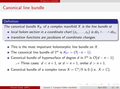
Definition
The canonical bundle KX of a complex manifold X is the line bundle st
local holom section in a coordinate chart (z1, . . . , zn) is dz1∧ · · ·∧dzn;
transition functions are jacobians of coordinate changes.
This is the most important holomorphic line bundle on X .
The canonical line bundle of Pn is KPn = O(−n − 1).
Canonical bundle of hypersurface of degree d in Pn is O(d − n − 1).
↪→ Three cases: d < n + 1, or d = n + 1, orelse d > n + 1.
Canonical bundle of a complex torus X = Cn/Λ is 0 (i.e. X × C).
Canonical bundle of a product: KX1×X2 = π∗1KX1 ⊗ π∗2KX2 .
Vincent Guedj (IMT) Lecture 1: Compact Kahler manifolds April 2021 12 / 19

Projective manifolds
Canonical line bundle
Definition
The canonical bundle KX of a complex manifold X is the line bundle st
local holom section in a coordinate chart (z1, . . . , zn) is dz1∧ · · ·∧dzn;
transition functions are jacobians of coordinate changes.
This is the most important holomorphic line bundle on X .
The canonical line bundle of Pn is KPn = O(−n − 1).
Canonical bundle of hypersurface of degree d in Pn is O(d − n − 1).
↪→ Three cases: d < n + 1, or d = n + 1, orelse d > n + 1.
Canonical bundle of a complex torus X = Cn/Λ is 0 (i.e. X × C).
Canonical bundle of a product: KX1×X2 = π∗1KX1 ⊗ π∗2KX2 .
Vincent Guedj (IMT) Lecture 1: Compact Kahler manifolds April 2021 12 / 19

Projective manifolds
Curvature of holomorphic line bundles
Given s = {sU} ∈ H0(X , L), can measure the size of s(x) ∈ Lx by usingmetric h = {hU}
with hU = e−ϕU st ϕV = ϕU + log |gUV | setting
|s|h(x) := |sU(x)|e−ϕU(x) = |sV (x)|e−ϕV (x).
Definition
The curvature of the metric h is Θh := i∂∂ϕU = i∂∂ϕV . A line bundle ispositive if it admits a smooth metric whose curvature is a Kahler form.
Theorem (Kodaira embeding theorem)
A cpct complex manifold X is projective iff it admits a positive linebundle. In other words: L→ X is positive iff it is ample.
”Proof”: Lj very ample ⇒ Lj = φ∗LjO(1) has a Fubini-Study type metric.
Converse more delicate, can be proved by Hormander’s L2 techniques. �
Vincent Guedj (IMT) Lecture 1: Compact Kahler manifolds April 2021 13 / 19

Projective manifolds
Curvature of holomorphic line bundles
Given s = {sU} ∈ H0(X , L), can measure the size of s(x) ∈ Lx by usingmetric h = {hU} with hU = e−ϕU st ϕV = ϕU + log |gUV |
setting
|s|h(x) := |sU(x)|e−ϕU(x) = |sV (x)|e−ϕV (x).
Definition
The curvature of the metric h is Θh := i∂∂ϕU = i∂∂ϕV . A line bundle ispositive if it admits a smooth metric whose curvature is a Kahler form.
Theorem (Kodaira embeding theorem)
A cpct complex manifold X is projective iff it admits a positive linebundle. In other words: L→ X is positive iff it is ample.
”Proof”: Lj very ample ⇒ Lj = φ∗LjO(1) has a Fubini-Study type metric.
Converse more delicate, can be proved by Hormander’s L2 techniques. �
Vincent Guedj (IMT) Lecture 1: Compact Kahler manifolds April 2021 13 / 19

Projective manifolds
Curvature of holomorphic line bundles
Given s = {sU} ∈ H0(X , L), can measure the size of s(x) ∈ Lx by usingmetric h = {hU} with hU = e−ϕU st ϕV = ϕU + log |gUV | setting
|s|h(x) := |sU(x)|e−ϕU(x) = |sV (x)|e−ϕV (x).
Definition
The curvature of the metric h is Θh := i∂∂ϕU = i∂∂ϕV .
A line bundle ispositive if it admits a smooth metric whose curvature is a Kahler form.
Theorem (Kodaira embeding theorem)
A cpct complex manifold X is projective iff it admits a positive linebundle. In other words: L→ X is positive iff it is ample.
”Proof”: Lj very ample ⇒ Lj = φ∗LjO(1) has a Fubini-Study type metric.
Converse more delicate, can be proved by Hormander’s L2 techniques. �
Vincent Guedj (IMT) Lecture 1: Compact Kahler manifolds April 2021 13 / 19

Projective manifolds
Curvature of holomorphic line bundles
Given s = {sU} ∈ H0(X , L), can measure the size of s(x) ∈ Lx by usingmetric h = {hU} with hU = e−ϕU st ϕV = ϕU + log |gUV | setting
|s|h(x) := |sU(x)|e−ϕU(x) = |sV (x)|e−ϕV (x).
Definition
The curvature of the metric h is Θh := i∂∂ϕU = i∂∂ϕV . A line bundle ispositive if it admits a smooth metric whose curvature is a Kahler form.
Theorem (Kodaira embeding theorem)
A cpct complex manifold X is projective iff it admits a positive linebundle. In other words: L→ X is positive iff it is ample.
”Proof”: Lj very ample ⇒ Lj = φ∗LjO(1) has a Fubini-Study type metric.
Converse more delicate, can be proved by Hormander’s L2 techniques. �
Vincent Guedj (IMT) Lecture 1: Compact Kahler manifolds April 2021 13 / 19

Projective manifolds
Curvature of holomorphic line bundles
Given s = {sU} ∈ H0(X , L), can measure the size of s(x) ∈ Lx by usingmetric h = {hU} with hU = e−ϕU st ϕV = ϕU + log |gUV | setting
|s|h(x) := |sU(x)|e−ϕU(x) = |sV (x)|e−ϕV (x).
Definition
The curvature of the metric h is Θh := i∂∂ϕU = i∂∂ϕV . A line bundle ispositive if it admits a smooth metric whose curvature is a Kahler form.
Theorem (Kodaira embeding theorem)
A cpct complex manifold X is projective iff it admits a positive linebundle.
In other words: L→ X is positive iff it is ample.
”Proof”: Lj very ample ⇒ Lj = φ∗LjO(1) has a Fubini-Study type metric.
Converse more delicate, can be proved by Hormander’s L2 techniques. �
Vincent Guedj (IMT) Lecture 1: Compact Kahler manifolds April 2021 13 / 19

Projective manifolds
Curvature of holomorphic line bundles
Given s = {sU} ∈ H0(X , L), can measure the size of s(x) ∈ Lx by usingmetric h = {hU} with hU = e−ϕU st ϕV = ϕU + log |gUV | setting
|s|h(x) := |sU(x)|e−ϕU(x) = |sV (x)|e−ϕV (x).
Definition
The curvature of the metric h is Θh := i∂∂ϕU = i∂∂ϕV . A line bundle ispositive if it admits a smooth metric whose curvature is a Kahler form.
Theorem (Kodaira embeding theorem)
A cpct complex manifold X is projective iff it admits a positive linebundle. In other words: L→ X is positive iff it is ample.
”Proof”: Lj very ample ⇒ Lj = φ∗LjO(1) has a Fubini-Study type metric.
Converse more delicate, can be proved by Hormander’s L2 techniques. �
Vincent Guedj (IMT) Lecture 1: Compact Kahler manifolds April 2021 13 / 19

Projective manifolds
Curvature of holomorphic line bundles
Given s = {sU} ∈ H0(X , L), can measure the size of s(x) ∈ Lx by usingmetric h = {hU} with hU = e−ϕU st ϕV = ϕU + log |gUV | setting
|s|h(x) := |sU(x)|e−ϕU(x) = |sV (x)|e−ϕV (x).
Definition
The curvature of the metric h is Θh := i∂∂ϕU = i∂∂ϕV . A line bundle ispositive if it admits a smooth metric whose curvature is a Kahler form.
Theorem (Kodaira embeding theorem)
A cpct complex manifold X is projective iff it admits a positive linebundle. In other words: L→ X is positive iff it is ample.
”Proof”: Lj very ample ⇒ Lj = φ∗LjO(1) has a Fubini-Study type metric.
Converse more delicate, can be proved by Hormander’s L2 techniques. �
Vincent Guedj (IMT) Lecture 1: Compact Kahler manifolds April 2021 13 / 19

Projective manifolds
First Chern class
The transition functions gUV of a holomorphic line bundle L→ X satisfy
gUV · gVU = 1 and gUV · gVW · gWU = 1.
↪→ class in H1(X ,O∗)=set of holomorphic line bdles modulo isom .
Definition (First Chern class)
The Chern class c1(L) is the image L ∈ H1(X ,O∗) 7→ c1(L) ∈ H2(X ,Z)under the map induced by the exact sequence 0→ Z→ O → O∗ → 0.
Analytically c1(L) ∈ H2(X ,Z) 7→ c(L) ∈ H2(X ,R) induced by Z ⊂ R.
Proposition
One has c(L) = {Θh} for any smooth hermitian metric h of L.
Definition
The first Chern class of X is c1(X ) = c1(−KX ).
Vincent Guedj (IMT) Lecture 1: Compact Kahler manifolds April 2021 14 / 19

Projective manifolds
Classification
Definition (-Proposition)
dimH0(X ,K jX ) ∼ jν where ν ∈ {−∞, 0, . . . , n} =Kodaira dimension.
The Kodaira dimension kod(X ) := ν is a (birational) invariant.
Example
If X is a compact Riemann surface (n = 1). Then
either kod(X ) = −∞⇔ KX is negative ⇔ X ∼ P1;
or kod(X ) = 0⇔ KX = 0 is trivial ⇔ X is an elliptic curve;
orelse kod(X ) = 1⇔ KX is positive ⇔ X is hyperbolic.
The classification in dimension n = 2 is (almost) complete.
In higher dimension n ≥ 3 needs to consider singular models (MMP).
↪→ Seeking for canonical Kahler metrics might help (next Lectures).
Vincent Guedj (IMT) Lecture 1: Compact Kahler manifolds April 2021 15 / 19

Projective manifolds
Classification
Definition (-Proposition)
dimH0(X ,K jX ) ∼ jν where ν ∈ {−∞, 0, . . . , n} =Kodaira dimension.
The Kodaira dimension kod(X ) := ν is a (birational) invariant.
Example
If X is a compact Riemann surface (n = 1).
Then
either kod(X ) = −∞⇔ KX is negative ⇔ X ∼ P1;
or kod(X ) = 0⇔ KX = 0 is trivial ⇔ X is an elliptic curve;
orelse kod(X ) = 1⇔ KX is positive ⇔ X is hyperbolic.
The classification in dimension n = 2 is (almost) complete.
In higher dimension n ≥ 3 needs to consider singular models (MMP).
↪→ Seeking for canonical Kahler metrics might help (next Lectures).
Vincent Guedj (IMT) Lecture 1: Compact Kahler manifolds April 2021 15 / 19

Projective manifolds
Classification
Definition (-Proposition)
dimH0(X ,K jX ) ∼ jν where ν ∈ {−∞, 0, . . . , n} =Kodaira dimension.
The Kodaira dimension kod(X ) := ν is a (birational) invariant.
Example
If X is a compact Riemann surface (n = 1). Then
either kod(X ) = −∞⇔ KX is negative ⇔ X ∼ P1;
or kod(X ) = 0⇔ KX = 0 is trivial ⇔ X is an elliptic curve;
orelse kod(X ) = 1⇔ KX is positive ⇔ X is hyperbolic.
The classification in dimension n = 2 is (almost) complete.
In higher dimension n ≥ 3 needs to consider singular models (MMP).
↪→ Seeking for canonical Kahler metrics might help (next Lectures).
Vincent Guedj (IMT) Lecture 1: Compact Kahler manifolds April 2021 15 / 19

Projective manifolds
Classification
Definition (-Proposition)
dimH0(X ,K jX ) ∼ jν where ν ∈ {−∞, 0, . . . , n} =Kodaira dimension.
The Kodaira dimension kod(X ) := ν is a (birational) invariant.
Example
If X is a compact Riemann surface (n = 1). Then
either kod(X ) = −∞⇔ KX is negative ⇔ X ∼ P1;
or kod(X ) = 0⇔ KX = 0 is trivial ⇔ X is an elliptic curve;
orelse kod(X ) = 1⇔ KX is positive ⇔ X is hyperbolic.
The classification in dimension n = 2 is (almost) complete.
In higher dimension n ≥ 3 needs to consider singular models (MMP).
↪→ Seeking for canonical Kahler metrics might help (next Lectures).
Vincent Guedj (IMT) Lecture 1: Compact Kahler manifolds April 2021 15 / 19
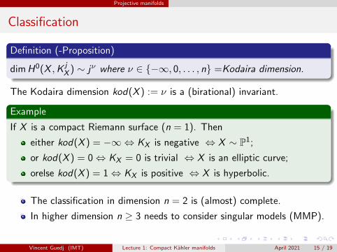
Projective manifolds
Classification
Definition (-Proposition)
dimH0(X ,K jX ) ∼ jν where ν ∈ {−∞, 0, . . . , n} =Kodaira dimension.
The Kodaira dimension kod(X ) := ν is a (birational) invariant.
Example
If X is a compact Riemann surface (n = 1). Then
either kod(X ) = −∞⇔ KX is negative ⇔ X ∼ P1;
or kod(X ) = 0⇔ KX = 0 is trivial ⇔ X is an elliptic curve;
orelse kod(X ) = 1⇔ KX is positive ⇔ X is hyperbolic.
The classification in dimension n = 2 is (almost) complete.
In higher dimension n ≥ 3 needs to consider singular models (MMP).
↪→ Seeking for canonical Kahler metrics might help (next Lectures).Vincent Guedj (IMT) Lecture 1: Compact Kahler manifolds April 2021 15 / 19

Curvatures
Scalar and Ricci curvatures
Let (X , ω) be a compact Kahler manifold,
ωloc=∑
α,β gαβ idzα ∧ dzβ.
Definition
The Ricci form of ω is Ric(ω) = − 1π
∑ ∂2 log det(gpq)∂zα∂zβ
idzα ∧ dzβ.
The scalar curvature of ω is Scal(ω) =: Trω(Ric(ω)) = nRic(ω)∧ωn−1
ωn .
Ric(ω) =globally well defined closed (1, 1)-form.
Ric(η) = Ric(ω)− ddc(ηn
ωn
), with ddc = i
π∂∂.
Proposition
The cohomology class of Ric(ω) is c1(X ) = −c1(KX ).
Vincent Guedj (IMT) Lecture 1: Compact Kahler manifolds April 2021 16 / 19

Curvatures
Scalar and Ricci curvatures
Let (X , ω) be a compact Kahler manifold, ωloc=∑
α,β gαβ idzα ∧ dzβ.
Definition
The Ricci form of ω is Ric(ω) = − 1π
∑ ∂2 log det(gpq)∂zα∂zβ
idzα ∧ dzβ.
The scalar curvature of ω is Scal(ω) =: Trω(Ric(ω)) = nRic(ω)∧ωn−1
ωn .
Ric(ω) =globally well defined closed (1, 1)-form.
Ric(η) = Ric(ω)− ddc(ηn
ωn
), with ddc = i
π∂∂.
Proposition
The cohomology class of Ric(ω) is c1(X ) = −c1(KX ).
Vincent Guedj (IMT) Lecture 1: Compact Kahler manifolds April 2021 16 / 19

Curvatures
Kahler-Einstein and cscK metrics
Definition
A Kahler metric is Kahler-Einstein if there exists λ ∈ R st Ric(ω) = λω.
A Kahler metric has constant scalar curvature if Scal(ω) ≡ cst.
Clearly Kahler-Einstein ⇒ cscK.
Converse is true if c1(X ) = λ{ω} (Exercise).
Can rescale to λ ∈ {−1, 0,+1} since Ric(εω) = Ric(ω).
Existence of K-E necessitates that c1(X ) has a sign.
Not always true (X = S1 × S2) but building blocks of classification.
↪→ Constructing K-E metrics is a main goal of these lectures.
Vincent Guedj (IMT) Lecture 1: Compact Kahler manifolds April 2021 17 / 19

Curvatures
Kahler-Einstein and cscK metrics
Definition
A Kahler metric is Kahler-Einstein if there exists λ ∈ R st Ric(ω) = λω.A Kahler metric has constant scalar curvature if Scal(ω) ≡ cst.
Clearly Kahler-Einstein ⇒ cscK.
Converse is true if c1(X ) = λ{ω} (Exercise).
Can rescale to λ ∈ {−1, 0,+1} since Ric(εω) = Ric(ω).
Existence of K-E necessitates that c1(X ) has a sign.
Not always true (X = S1 × S2) but building blocks of classification.
↪→ Constructing K-E metrics is a main goal of these lectures.
Vincent Guedj (IMT) Lecture 1: Compact Kahler manifolds April 2021 17 / 19
Curvatures
Examples
Example
The flat metric ω =∑
idzα ∧ dzβ on X = Cn/Λ satisfies Ric(ω) = 0.
Example
The Fubini-Study metric ω = ddc log[1 + |z |2] on Pn satisfies
ωαβ =δαβ
[1 + |z |2]−
zαzβ[1 + |z |2]2
hence log det(ωαβ) = log 1[1+|z|2]n+1 = −(n + 1) log[1 + |z |2] yields
Ric(ω) = (n + 1)ω.
↪→ Many more (non explicit) examples in next Lectures.
Vincent Guedj (IMT) Lecture 1: Compact Kahler manifolds April 2021 18 / 19

Curvatures
Examples
Example
The flat metric ω =∑
idzα ∧ dzβ on X = Cn/Λ satisfies Ric(ω) = 0.
Example
The Fubini-Study metric ω = ddc log[1 + |z |2] on Pn
satisfies
ωαβ =δαβ
[1 + |z |2]−
zαzβ[1 + |z |2]2
hence log det(ωαβ) = log 1[1+|z|2]n+1 = −(n + 1) log[1 + |z |2] yields
Ric(ω) = (n + 1)ω.
↪→ Many more (non explicit) examples in next Lectures.
Vincent Guedj (IMT) Lecture 1: Compact Kahler manifolds April 2021 18 / 19

Curvatures
Examples
Example
The flat metric ω =∑
idzα ∧ dzβ on X = Cn/Λ satisfies Ric(ω) = 0.
Example
The Fubini-Study metric ω = ddc log[1 + |z |2] on Pn satisfies
ωαβ =δαβ
[1 + |z |2]−
zαzβ[1 + |z |2]2
hence log det(ωαβ) = log 1[1+|z|2]n+1 = −(n + 1) log[1 + |z |2] yields
Ric(ω) = (n + 1)ω.
↪→ Many more (non explicit) examples in next Lectures.
Vincent Guedj (IMT) Lecture 1: Compact Kahler manifolds April 2021 18 / 19

Curvatures
Examples
Example
The flat metric ω =∑
idzα ∧ dzβ on X = Cn/Λ satisfies Ric(ω) = 0.
Example
The Fubini-Study metric ω = ddc log[1 + |z |2] on Pn satisfies
ωαβ =δαβ
[1 + |z |2]−
zαzβ[1 + |z |2]2
hence log det(ωαβ) = log 1[1+|z|2]n+1 = −(n + 1) log[1 + |z |2]
yields
Ric(ω) = (n + 1)ω.
↪→ Many more (non explicit) examples in next Lectures.
Vincent Guedj (IMT) Lecture 1: Compact Kahler manifolds April 2021 18 / 19

Curvatures
Examples
Example
The flat metric ω =∑
idzα ∧ dzβ on X = Cn/Λ satisfies Ric(ω) = 0.
Example
The Fubini-Study metric ω = ddc log[1 + |z |2] on Pn satisfies
ωαβ =δαβ
[1 + |z |2]−
zαzβ[1 + |z |2]2
hence log det(ωαβ) = log 1[1+|z|2]n+1 = −(n + 1) log[1 + |z |2] yields
Ric(ω) = (n + 1)ω.
↪→ Many more (non explicit) examples in next Lectures.
Vincent Guedj (IMT) Lecture 1: Compact Kahler manifolds April 2021 18 / 19

Curvatures
Examples
Example
The flat metric ω =∑
idzα ∧ dzβ on X = Cn/Λ satisfies Ric(ω) = 0.
Example
The Fubini-Study metric ω = ddc log[1 + |z |2] on Pn satisfies
ωαβ =δαβ
[1 + |z |2]−
zαzβ[1 + |z |2]2
hence log det(ωαβ) = log 1[1+|z|2]n+1 = −(n + 1) log[1 + |z |2] yields
Ric(ω) = (n + 1)ω.
↪→ Many more (non explicit) examples in next Lectures.
Vincent Guedj (IMT) Lecture 1: Compact Kahler manifolds April 2021 18 / 19

References
A few references
F.ZhengComplex differential geometry,International Press, Boston, MA, 2000.
R.LazarsfeldPositivity in Algebraic Geometry. I,Springer-Verlag, Berlin, 2004.
C.Voisin,Hodge theory and complex algebraic geometry. I,Cambridge University Press, Cambridge, 2007.
G.Szekelyhidi,An Introduction to Extremal Kahler Metrics.,Graduate Studies in Mathematics, AMS, 2014.
Vincent Guedj (IMT) Lecture 1: Compact Kahler manifolds April 2021 19 / 19