lecture 1 - api.ning.com will in c++ and you will generate intel x86 assembly language ... parser...
TRANSCRIPT

Sohail Aslam Compiler Construction Notes
1
LLeeccttuurree 11
Course Organization
The course is organized around theory and significant amount of practice. The practice will be in the form of home works and a project. The project is the highlight of the course: you will build a full compiler for subset of Java- like language. The implementation will in C++ and you will generate Intel x86 assembly language code. The project will be done in six parts; each will be a programming assignment. The grade distribution will be
The primary text for the course is Compilers – Principles, Techniques and Tools by Aho, Sethi and Ullman. This is also called the Dragon Book; here is the image on the cover of the book:
Theory Homeworks 10%
Exams 50%
Practice Project 40%

Sohail Aslam Compiler Construction Notes
2
Why Take this Course
There are number of reason for why you should take this course. Let’s go through a few Reason #1: understand compilers and languages We all have used one or computer languages to write programs. We have used compilers to “compile” our code and eventually turn it into an executable. While we worry about data structures, algorithms and all the functionality that our application is supposed to provide, we perhaps overlook the programming language, the structure of the code and the language semantics. In this course, we will attempt to understand the code structure, understand language semantics and understand relation between source code and generated machine code. This will allow you to become a better programmer Reason #2: nice balance of theory and practice We have studied a lot of theory in various CS courses related to languages and grammar. We have covered mathematical models: regular expressions, automata, grammars and graph algorithms that use these models. We will now have an opportunity to put this theory into practice by building a real compiler. Reason #3: programming experience Creating a compiler entails writing a large computer program which manipulates complex data structures and implement sophisticated algorithm. In the process, we will learn more about C++ and Intel x86 assembly language. The experience, however, will be applicable if we desire to use another programming language, say Java, and generate code for architecture other than Intel.
What are Compilers
Compilers translate information from one representation to another. Thus, a tool that translates, say, Russian into English could be labeled as a compiler. In this course, however, information = program in a computer language. In this context, we will talk of compilers such as VC, VC++, GCC, JavaC FORTRAN, Pascal, VB. Application that convert, for example, a Word file to PDF or PDF to Postscript will be called “translators”. In this course we will study typical compilation: from programs written in high- level languages to low-level object code and machine code.

Sohail Aslam Compiler Construction Notes
3
Typical Compilation
Consider the source code of C function int expr( int n ) { int d; d = 4*n*n*(n+1)*(n+1); return d; } Expressing an algorithm or a task in C is optimized for human readability and comprehension. This presentation matches human notions of grammar of a programming language. The function uses named constructs such as variables and procedures which aid human readability. Now consider the assembly code that the C compiler gcc generates for the Intel platform: .globl _expr _expr: pushl %ebp movl %esp,%ebp subl $24,%esp movl 8(%ebp),%eax movl %eax,%edx leal 0(,%edx,4),%eax movl %eax,%edx imull 8(%ebp),%edx movl 8(%ebp),%eax incl %eax imull %eax,%edx movl 8(%ebp),%eax incl %eax imull %eax,%edx movl %edx,-4(%ebp) movl -4(%ebp),%edx movl %edx,%eax jmp L2 .align 4 L2: leave ret The assembly code is optimized for hardware it is to run on. The code consists of machine instructions, uses registers and unnamed memory locations. This version is much harder to understand by humans

Sohail Aslam Compiler Construction Notes
4
Issues in Compilation
The translation of code from some human readable form to machine code must be “correct”, i.e., the generated machine code must execute precisely the same computation as the source code. In general, there is no unique translation from source language to a destination language. No algorithm exists for an “ideal translation”. Translation is a complex process. The source language and generated code are very different. To manage this complex process, the translation is carried out in multiple passes.

Sohail Aslam Compiler Construction Notes
1
LLeeccttuurree 22
Two-pass Compiler
The figure above shows the structure of a two-pass compiler. The front end maps legal source code into an intermediate representation (IR). The back end maps IR into target machine code. An immediate advantage of this scheme is that it admits multiple front ends and multiple passes. The algorithms employed in the front end have polynomial time complexity while majority of those in the backend are NP-complete. This makes compiler writing a challenging task. Let us look at the details of the front and back ends. Front End
scanner parsersourcecode
tokens IR
errors
The front end recognizes legal and illegal programs presented to it. When it encounters errors, it attempts to report errors in a useful way. For legal programs, front end produces IR and preliminary storage map for the various data structures declared in the program. The front end consists of two modules:
1. Scanner 2. Parser

Sohail Aslam Compiler Construction Notes
2
Scanner
The scanner takes a program as input and maps the character stream into “words” that are the basic unit of syntax. It produces pairs – a word and its part of speech. For example, the input x = x + y becomes <id,x> <assign,=> <id,x> <op,+> <id,y> We call the pair “<token type, word>” a token. Typical tokens are: number, identifier, +, -, new, while, if. Parser
The parser takes in the stream of tokens, recognizes context- free syntax and reports errors. It guides context-sensitive (“semantic”) analysis for tasks like type checking. The parser builds IR for source program. The syntax of most programming languages is specified using Context-Free Grammars (CFG). Context- free syntax is specified with a grammar G=(S,N,T,P) where
• S is the start symbol • N is a set of non-terminal symbols • T is set of terminal symbols or words • P is a set of productions or rewrite rules
For example, the Context-Free Grammar for arithmetic expressions is
1. goal ? expr 2. expr ? expr op term 3. | term 4. term ? number 5. | id 6. op ? + 7. | –
For this CFG,
S = goal

Sohail Aslam Compiler Construction Notes
3
T = { number, id, +, -} N = { goal, expr, term, op} P = { 1, 2, 3, 4, 5, 6, 7}
Given a CFG, we can derive sentences by repeated substitution. Consider the sentence x + 2 – y
Production Result
goal
1: goal ? expr expr
2: expr ? expr op term expr op term
5: term ? id expr op y
7: op ? – expr – y
2: expr ? expr op term expr op term – y
4: term ? number expr op 2 – y
6: op ? + expr + 2 – y
3: expr ? term term + 2 – y
5: term ? id x + 2 – y
To recognize a valid sentence in some CFG, we reverse this process and build up a parse, thus the name “parser”.

Sohail Aslam Compiler Construction Notes
1
LLeeccttuurree 33
A parse can be represented by a tree: parse tree or syntax tree. For example, here is the parse tree for the expression x+2-y
The parse tree captures all rewrite during the derivation. The derivation can be extracted by starting at the root of the tree and working towards the leaf nodes. Abstract Syntax Trees
The parse tree contains a lot of unneeded information. Compilers often use an abstract syntax tree (AST). For example, the AST for the above parse tree is
This is much more concise; AST summarizes grammatical structure without the details of derivation. ASTs are one kind of intermediate representation (IR). The Back End
–
<id,y>
<id,x> <number,2>
+

Sohail Aslam Compiler Construction Notes
2
The back end of the compiler translates IR into target machine code. It chooses machine (assembly) instructions to implement each IR operation. The back end ensure conformance with system interfaces. It decides which values to keep in registers in order to avoid memory access; memory access is far slower than register access.
The back end is responsible for instruction selection so as to produce fast and compact code. Modern processors have a rich instruction set. The back end takes advantage of target features such as addressing modes. Usually, instruction selection is viewed as a pattern matching problem that can be solved by dynamic programming based algorithms. Instruction selection in compilers was spurred by the advent of the VAX-11 which had a CISC (Complex Instruction Set Computer) architecture. The VAX-11 had a large instruction set that the compiler could work with.

Sohail Aslam Compiler Construction Notes
1
LLeeccttuurree 44
CISC architecture provided a rich set of instructions and addressing modes but it made the job of the compiler harder when it came to generate efficient machine code. The RISC architecture simplified this problem. Register Allocation
Registers in a CPU play an important role for providing high speed access to operands. Memory access is an order of magnitude slower than register access. The back end attempts to have each operand value in a register when it is used. However, the back end has to manage a limited set of resources when it comes to the register file. The number of registers is small and some registers are pre-allocated for specialize used, e.g., program counter, and thus are not available for use to the back end. Optimal register allocation is NP-Complete. Instruction Scheduling
Modern processors have multiple functional units. The back end needs to schedule instructions to avoid hardware stalls and interlocks. The generated code should use all functional units productively. Optimal scheduling is NP-Complete in nearly all cases. Three-pass Compiler
There is yet another opportunity to produce efficient translation: most modern compilers contain three stages. An intermediate stage is used for code improvement or optimization. The topology of a three-pass compiler is shown in the following figure:
FrontEnd
machinecode
errors
MiddleEnd
BackEnd
IR IR
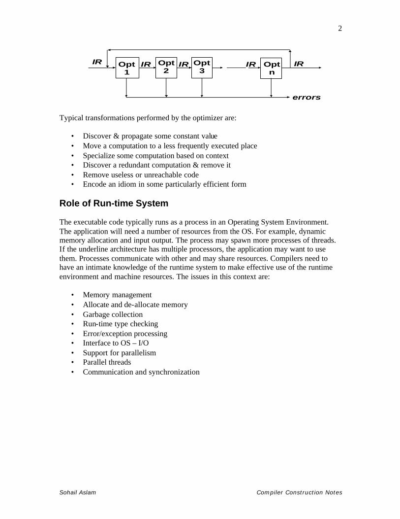
The middle end analyzes IR and rewrites (or transforms) IR. Its primary goal is to reduce running time of the compiled code. This may also improve space usage, power consumption, etc. The middle end is generally termed the “Optimizer”. Modern optimizers are structured as a series of passes:
Sohail Aslam Compiler Construction Notes
2
Opt1
IR IR
errors
Opt2
Optn
IR IR Opt3
IR
Typical transformations performed by the optimizer are:
• Discover & propagate some constant value • Move a computation to a less frequently executed place • Specialize some computation based on context • Discover a redundant computation & remove it • Remove useless or unreachable code • Encode an idiom in some particularly efficient form
Role of Run-time System
The executable code typically runs as a process in an Operating System Environment. The application will need a number of resources from the OS. For example, dynamic memory allocation and input output. The process may spawn more processes of threads. If the underline architecture has multiple processors, the application may want to use them. Processes communicate with other and may share resources. Compilers need to have an intimate knowledge of the runtime system to make effective use of the runtime environment and machine resources. The issues in this context are:
• Memory management • Allocate and de-allocate memory • Garbage collection • Run-time type checking • Error/exception processing • Interface to OS – I/O • Support for parallelism • Parallel threads • Communication and synchronization

Sohail Aslam Compiler Construction Notes
1
LLeeccttuurree 55
Lexical Analysis
The scanner is the first component of the front-end of a compiler; parser is the second
scanner parsersourcecode
tokens IR
errors
The task of the scanner is to take a program written in some programming language as a stream of characters and break it into a stream of tokens. This activity is called lexical analysis. A token, however, contains more than just the words extracted from the input. The lexical analyzer partition input string into substrings, called words, and classifies them according to their role. Tokens
A token is a syntactic category in a sentence of a language. Consider the sentence: He wrote the program
of the natural language English. The words in the sentence are: “He”, “wrote”, “the” and “program”. The blanks between words have been ignored. These words are classified as subject, verb, object etc. These are the roles. Similarly, the sentence in a programming language like C: if(b == 0) a = b the words are “if”, “(”, “b”, “==”, “0”, “)”, “a”, “=” and “b”. The roles are keyword, variable, boolean operator, assignment operator. The pair <role,word> is given the name token. Here are some familiar tokens in programming languages:
• Identifiers: x y11 maxsize • Keywords: if else while for • Integers: 2 1000 -44 5L • Floats: 2.0 0.0034 1e5 • Symbols: ( ) + * / { } < > == • Strings: “enter x” “error”

Sohail Aslam Compiler Construction Notes
2
Ad-hoc Lexer
The task of writing a scanner is fairly straight forward. We can hand-write code to generate tokens. We do this by partitioning the input string by reading left-to-right, recognizing one token at a time. We will need to look-ahead in order to decide where one token ends and the next token begins. The following C++ code present is template for a Lexer class. An object of this class can produce the desired tokens from the input stream. class Lexer {
Inputstream s; char next; //look ahead Lexer(Inputstream _s) {
s = _s; next = s.read(); }
Token nextToken() {
if( idChar(next) )return readId(); if( number(next) )return readNumber(); if( next == ‘”’ ) return readString(); ... ...
} Token readId() {
string id = “”; while(true){
char c = input.read(); if(idChar(c) == false)
return new Token(TID,id); id = id + string(c);
} } boolean idChar(char c) {
if( isAlpha(c) ) return true; if( isDigit(c) ) return true; if( c == ‘_’ ) return true;
return false;
} Token readNumber(){
string num = “”; while(true){

Sohail Aslam Compiler Construction Notes
3
next = input.read(); if( !isNumber(next))
return new Token(TNUM,num); num = num+string(next);
} } This works ok, however, there are some problem that we need to tackle.
• We do not know what kind of token we are going to read from seeing first character.
• If token begins with “i”, is it an identifier “i” or keyword “if”? • If token begins with “=”, is it “=” or “==”?
We can extend the Lexer class but there are a number of other issues that can make the task of hand-writing a lexer tedious. We need a more principled approach. The most frequently used approach is to use a lexer generator that generates efficient tokenizer automatically.

Sohail Aslam Compiler Construction Notes
1
LLeeccttuurree 66
How to Describe Tokens?
Regular Languages are the most popular for specifying tokens because • These are based on simple and useful theory, • Are easy to understand and • Efficient implementations exist for generating lexical analysers based on such
languages. Languages
Let Σ ?be a set of characters. Σ is called the alphabet. A language over Σ is set of strings of characters drawn from Σ.? Here are some examples of languages:
• Alphabet = English characters Language = English sentences
• Alphabet = ASCII
Language = C++, Java, C# programs Languages are sets of strings (finite sequence of characters). We need some notation for specifying which sets we want. For lexical analysis we care about regular languages. Regular languages can be described using regular expressions. Each regular expression is a notation for a regular language (a set of words). If A is a regular expression, we write L(A) to refer to language denoted by A. Regular Expression
A regular expression (RE) is defined inductively a ordinary character from Σ ε the empty string
R|S either R or S RS R followed by S (concatenation) R* concatenation of R zero or more times (R* = ε |R|RR|RRR...)
Regular expression extensions are used as convenient notation of complex RE:
R? ε | R (zero or one R) R+ RR* (one or more R) (R) R (grouping) [abc] a|b|c (any of listed) [a-z] a|b|....|z (range) [^ab] c|d|... (anything but ‘a’‘b’)
Sohail Aslam Compiler Construction Notes
2
Here are some Regular Expressions and the strings of the language denoted by the RE.
RE Strings in L(R) a “a” ab “ab” a|b “a” “b” (ab)* “” “ab” “abab” ... (a|ε)b “ab” “b”
Here are examples of common tokens found in programming languages.
digit ‘0’|’1’|’2’|’3’|’4’|’5’|’6’|’7’|’8’|’9’ integer digit digit* identifier [a-zA-Z_][a-zA-Z0-9_]*
Finite Automaton
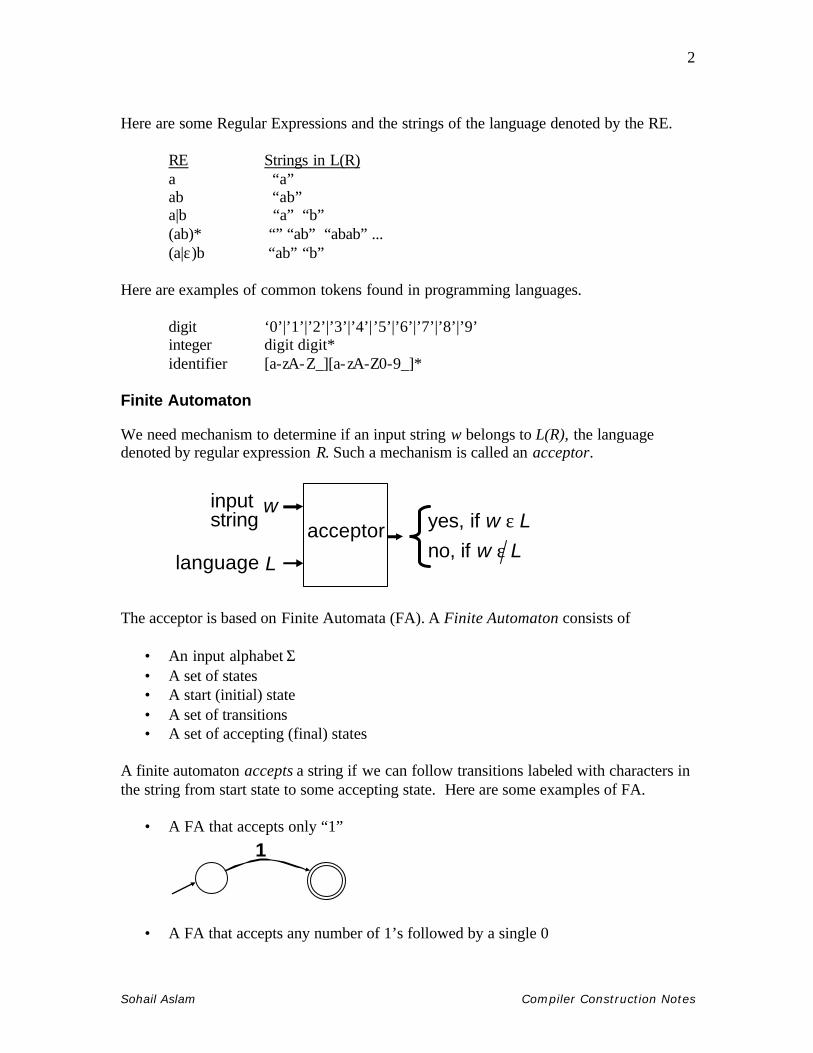
We need mechanism to determine if an input string w belongs to L(R), the language denoted by regular expression R. Such a mechanism is called an acceptor.
input string
language
w
L
acceptor yes, if w ε Lno, if w ε L
The acceptor is based on Finite Automata (FA). A Finite Automaton consists of
• An input alphabet Σ • A set of states • A start (initial) state • A set of transitions • A set of accepting (final) states
A finite automaton accepts a string if we can follow transitions labeled with characters in the string from start state to some accepting state. Here are some examples of FA.
• A FA that accepts only “1”
1
• A FA that accepts any number of 1’s followed by a single 0

Sohail Aslam Compiler Construction Notes
3
01
• A FA that accepts ab*a (Σ : {a,b})
a
b
a
Sohail Aslam Compiler Construction Notes
1
LLeeccttuurree 77
Table Encoding of FA
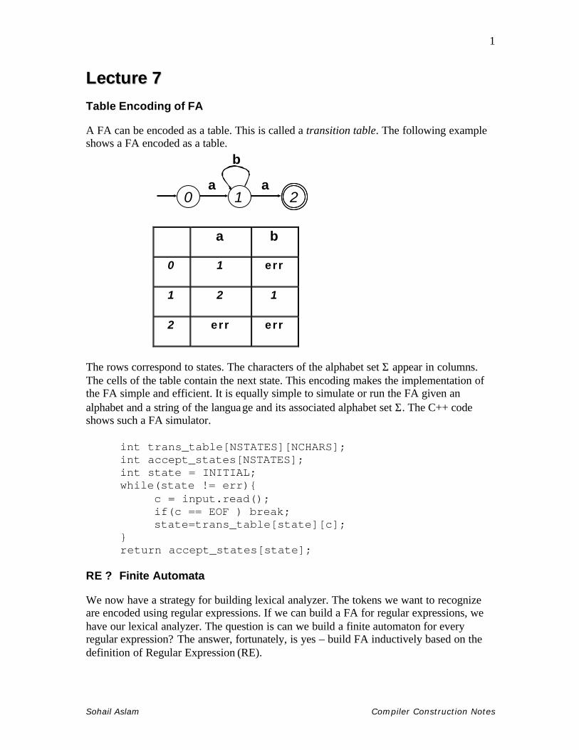
A FA can be encoded as a table. This is called a transition table. The following example shows a FA encoded as a table.
a
b
a0 1 2
a b
0 1 err
1 2 1
2 err err
The rows correspond to states. The characters of the alphabet set Σ appear in columns. The cells of the table contain the next state. This encoding makes the implementation of the FA simple and efficient. It is equally simple to simulate or run the FA given an alphabet and a string of the language and its associated alphabet set Σ. The C++ code shows such a FA simulator.
int trans_table[NSTATES][NCHARS]; int accept_states[NSTATES]; int state = INITIAL; while(state != err){
c = input.read(); if(c == EOF ) break; state=trans_table[state][c];
} return accept_states[state];
RE ? Finite Automata
We now have a strategy for building lexical analyzer. The tokens we want to recognize are encoded using regular expressions. If we can build a FA for regular expressions, we have our lexical analyzer. The question is can we build a finite automaton for every regular expression? The answer, fortunately, is yes – build FA inductively based on the definition of Regular Expression (RE).
Sohail Aslam Compiler Construction Notes
2
The actual algorithm actually builds Nondeterministic Finite Automaton (NFA) from RE. Each RE is converted into an NFA. NFA are joined together with ε-moves. The eventual NFA is then converted into a Deterministic Finite Automaton (DFA) which can be encoded as a transition table. Let us discuss how this happens. Nondeterministic Finite Automaton (NFA)
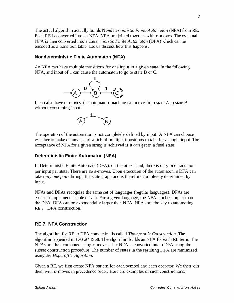
An NFA can have multiple transitions for one input in a given state. In the following NFA, and input of 1 can cause the automaton to go to state B or C.
1
1
0A B C
It can also have e–moves; the automaton machine can move from state A to state B without consuming input.
εA B
The operation of the automaton is not completely defined by input. A NFA can choose whether to make ε-moves and which of multiple transitions to take for a single input. The acceptance of NFA for a given string is achieved if it can get in a final state. Deterministic Finite Automaton (NFA)
In Deterministic Finite Automata (DFA), on the other hand, there is only one transition per input per state. There are no ε-moves. Upon execution of the automaton, a DFA can take only one path through the state graph and is therefore completely determined by input. NFAs and DFAs recognize the same set of languages (regular languages). DFAs are easier to implement – table driven. For a given language, the NFA can be simpler than the DFA. DFA can be exponentially larger than NFA. NFAs are the key to automating RE ? DFA construction. RE ? NFA Construction
The algorithm for RE to DFA conversion is called Thompson’s Construction. The algorithm appeared in CACM 1968. The algorithm builds an NFA for each RE term. The NFAs are then combined using ε-moves. The NFA is converted into a DFA using the subset construction procedure. The number of states in the resulting DFA are minimized using the Hopcroft’s algorithm. Given a RE, we first create NFA pattern for each symbol and each operator. We then join them with ε-moves in precedence order. Here are examples of such constructions:

Sohail Aslam Compiler Construction Notes
3
1. NFA for RE ab. The following figures show the construction steps. NFAs for RE a and RE b are made. These two are combined using an ε-move; the NFA for RE a appears on the left and is the source of the ε-transition.
ε
s0a
s1NFA for a
s0a s1
NFA for ab
s3b s4
s3b
s4NFA for b
εs0a s1
NFA for ab
s3b s4
2. NFA for RE a|b
εs0 s5
s1a s2
NFA for a | b
s3b s4ε
ε
ε
3. NFA for RE a*
εs0 s4s1a s2
NFA for a*
ε
ε
ε

Sohail Aslam Compiler Construction Notes
4
3. NFA for RE a ( b|c )* ε
s3 s9
s4 s5
s6 s7
s8s0 s1 s2a εε ε ε
ε ε
εb
c
ε

Sohail Aslam Compiler Construction Notes
1
LLeeccttuurree 88
NFA ? DFA Construction
The algorithm is called subset construction. In the transition table of an NFA, each entry is a set of states. In DFA, each entry is a single state. The general idea behind NFA-to-DFA construction is that each DFA state corresponds to a set of NFA states. The DFA uses its state to keep track of all possible states the NFA can be in after reading each input symbol. We will use the following operations.
• ε-closure(T): set of NFA states reachable from some NFA state s in T on ? -transitions alone.
• move(T,a): set of NFA states to which there is a transition on input a from some NFA state s in set of states T.
Before it sees the first input symbol, NFA can be in any of the state in the set ε-closure(s0), where s0 is the start state of the NFA. Suppose that exactly the states in set T are reachable from s0 on a given sequence of input symbols. Let a be the next input symbol. On seeing a, the NFA can move to any of the states in the set move(T,a). Let a be the next input symbol. On seeing a, the NFA can move to any of the states in the set move(T,a). When we allow for ε-transitions, NFA can be in any of the states in ε-closure(move(T,a)) after seeing a. Subset Construction
Algorithm: Input: NFA N with state set S, alphabet Σ, start state s0, final states F Output: DFA D with state set S’, alphabet Σ, start states, s0’ = ε-closure(s0), final states F’ and transition table: S’ x Σ ? S’ // initially, e-closure(s0) is the only state in D states S’ and it is unmarked s0’ = ε-closure(s0) S’ = {s0’ } (unmarked) while (there is some unmarked state T in S’)
mark state T for all a in Σ do
U = ? εclosure( move(T,a) ); if U not already in S’
add U as an unmarked state to S’ Dtran(T,a) = U;
end for end while

Sohail Aslam Compiler Construction Notes
2
F’: for each DFA state S
if S contains an NFA final state mark S as DFA final state
end algorithm Example Let us apply the algorithm to the NFA for (a | b )*abb. Σ is {a,b}.
0ε
ε
ε ε
εa
b
ε
ε
1
2 3
4 5
6 8 9ε
7 a b b10
The start state of equivalent DFA is ε-closure(0), which is A = {0,1,2,4,7}; these are exactly the states reachable from state 0 via ε-transition. The algorithm tells us to mark A and then compute ε-closure(move(A,a)) move(A,a)), is the set of states of NFA that have transition on ‘a’ from members of A. Only 2 and 7 have such transition, to 3 and 8. So, ε-closure(move(A,a)) = ε-closure({3,8}) = {1,2,3,4,6,7,8}. Let B = {1,2,3,4,6,7,8}; thus Dtran[A,a] = B For input b, among states in A, only 4 has transition on b to 5. Let C = ε-closure({5}) = {1,2,4,5,6,7}. Thus, Dtran[A,b] = C We continue this process with the unmarked sets B and C, i.e., ε-closure(move(B,a)), ε-closure(move(B,b)), ε-closure(move(C,a)) and ε-closure(move(C,b)) until all sets and states of DFA are marked. This is certain since there are only 211 (!) different subsets of a set of 11 states. A set, once marked, is marked forever. Eventually, the 5 sets are:
1. A={0,1,2,4,7} 2. B={1,2,3,4,6,7,8} 3. C={1,2,4,5,6,7} 4. D={1,2,4,5,6,7,9} 5. E={1,2,4,5,6,7,10}
A is start state because it contains state 0 and E is the accepting state because it contains state 10.

Sohail Aslam Compiler Construction Notes
3
The subset construction finally yields the following DFA
A
a
b a
b bEEB D
C
a
b
ba
a
The Resulting DFA can be encoded as the following transition table
CBEEBDCBCDBBCBAba
Input symbolState
CBEEBDCBCDBBCBAba
Input symbolState

Sohail Aslam Compiler Construction Notes
1
LLeeccttuurree 99
DFA Minimization
The generated DFA may have a large number of states. The Hopcroft’s algorithm can be used to minimize DFA states. The behind the algorithm is to find groups of equivalent states. All transitions from states in one group G1 go to states in the same group G2. Construct the minimized DFA such that there is one state for each group of states from the initial DFA. Here is the minimized version of the DFA created earlier; states A and C have been merged.
A,C
ab
b bEEB Da
b
a
a
We can construct an optimized acceptor with the following structure:
input string
RE
w
R
yes, if w ε L(R)
no, if w ε L(R)
RE=>NFA
NFA=>DFA
Min. DFA
SimulateDFA
Lexical Analyzers
Lexical analyzers (scanners) use the same mechanism but they have multiple RE descriptions for multiple tokens and have a character stream at the input. The lexical analyzer returns a sequence of matching tokens at the output (or an error) and it always return the longest matching token.

Sohail Aslam Compiler Construction Notes
2
Lexical Analyzer Generators
The process of constructing a lexical analyzer can automated. We only need to specify Regular expressions for tokens and rules for assigning priorities for multiple longest match cases, e.g, “==” and “=”, “==” is longer. Two popular lexical analyzer generators are
• Flex : generates lexical analyzer in C or C++. It is more modern version of the original Lex tool that was part of the AT&T Bell Labs version of Unix.
• Jlex: written in Java. Generates lexical analyzer in Java Using Flex
We will use for the projects in this course. To use Flex, one has to provide a specification file as input to Flex. Flex reads this file and produces an output file contains the lexical analyzer source in C or C++. The input specification file consists of three sections:
C or C++ and flex definitions %% token definitions and actions %% user code
The symbols “%%” mark each section. A detailed guide to Flex is included in supplementary reading material for this course. We will go through a simple example. The following is the Flex specification file for recognizing tokens found in a C++ function. The file is named “lex.l”; it is customary to use the “.l” extension for Flex input files.
%{ #include “tokdefs.h” %} D [0-9] L [a-zA-Z_] id {L}({L}|{D})* %% "void" {return(TOK_VOID);} "int" {return(TOK_INT);} "if" {return(TOK_IF);} Specification File lex.l "else" {return(TOK_ELSE);} "while"{return(TOK_WHILE)}; "<=" {return(TOK_LE);}

Sohail Aslam Compiler Construction Notes
3
">=" {return(TOK_GE);} "==" {return(TOK_EQ);} "!=" {return(TOK_NE);} {D}+ {return(TOK_INT);} {id} {return(TOK_ID);} [\n]|[\t]|[ ] ; %%
The file lex.l includes another file named “tokdefs.h”. The content of tokdefs.h are
#define TOK_VOID 1 #define TOK_INT 2 #define TOK_IF 3 #define TOK_ELSE 4 #define TOK_WHILE 5 #define TOK_LE 6 #define TOK_GE 7 #define TOK_EQ 8 #define TOK_NE 9 #define TOK_INT 10 #define TOK_ID 111
Flex creates C++ classes that implement the lexical analyzer. The code for these classes is placed in the Flex’s output file. Here, for example, is the code needed to invoke the scanner; this is placed in main.cpp:
void main() {
FlexLexer lex; int tc = lex.yylex(); while(tc != 0) {
cout << tc << “,” <<lex.YYText() << endl; tc = lex.yylex();
} }
The following commands can be used to generate a scanner executable file in windows.
flex lex.l g++ –c lex.cpp g++ –c main.cpp g++ –o lex.exe lex.o main.o
Sohail Aslam Compiler Construction Notes
1
LLeeccttuurree 1100
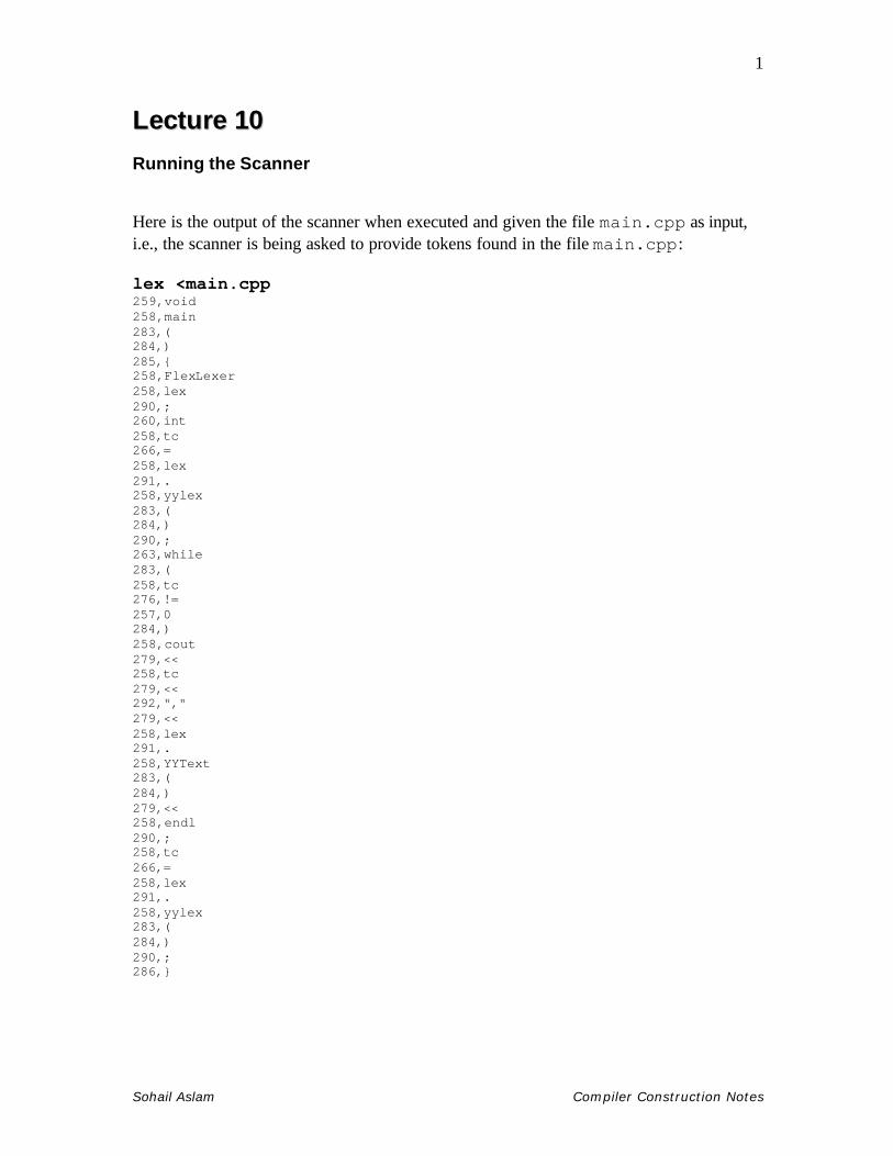
Running the Scanner
Here is the output of the scanner when executed and given the file main.cpp as input, i.e., the scanner is being asked to provide tokens found in the file main.cpp: lex <main.cpp 259,void 258,main 283,( 284,) 285,{ 258,FlexLexer 258,lex 290,; 260,int 258,tc 266,= 258,lex 291,. 258,yylex 283,( 284,) 290,; 263,while 283,( 258,tc 276,!= 257,0 284,) 258,cout 279,<< 258,tc 279,<< 292,"," 279,<< 258,lex 291,. 258,YYText 283,( 284,) 279,<< 258,endl 290,; 258,tc 266,= 258,lex 291,. 258,yylex 283,( 284,) 290,; 286,}
Sohail Aslam Compiler Construction Notes
2
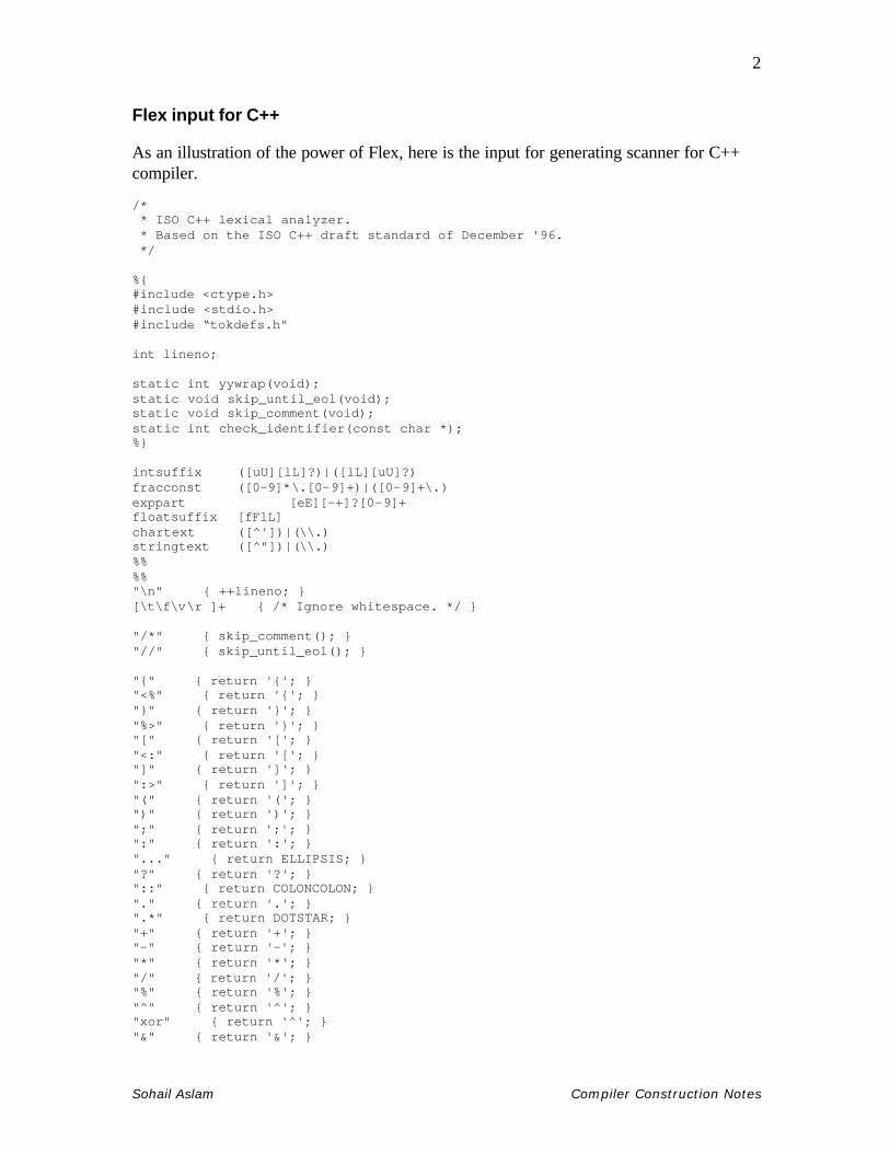
Flex input for C++
As an illustration of the power of Flex, here is the input for generating scanner for C++ compiler. /* * ISO C++ lexical analyzer. * Based on the ISO C++ draft standard of December '96. */ %{ #include <ctype.h> #include <stdio.h> #include “tokdefs.h" int lineno; static int yywrap(void); static void skip_until_eol(void); static void skip_comment(void); static int check_identifier(const char *); %} intsuffix ([uU][lL]?)|([lL][uU]?) fracconst ([0-9]*\.[0-9]+)|([0-9]+\.) exppart [eE][-+]?[0-9]+ floatsuffix [fFlL] chartext ([^'])|(\\.) stringtext ([^"])|(\\.) %% %% "\n" { ++lineno; } [\t\f\v\r ]+ { /* Ignore whitespace. */ } "/*" { skip_comment(); } "//" { skip_until_eol(); } "{" { return '{'; } "<%" { return '{'; } "}" { return '}'; } "%>" { return '}'; } "[" { return '['; } "<:" { return '['; } "]" { return ']'; } ":>" { return ']'; } "(" { return '('; } ")" { return ')'; } ";" { return ';'; } ":" { return ':'; } "..." { return ELLIPSIS; } "?" { return '?'; } "::" { return COLONCOLON; } "." { return '.'; } ".*" { return DOTSTAR; } "+" { return '+'; } "-" { return '-'; } "*" { return '*'; } "/" { return '/'; } "%" { return '%'; } "^" { return '^'; } "xor" { return '^'; } "&" { return '&'; }

Sohail Aslam Compiler Construction Notes
3
"bitand" { return '&'; } "|" { return '|'; } "bitor" { return '|'; } "~" { return '~'; } "compl" { return '~'; } "!" { return '!'; } "not" { return '!'; } "=" { return '='; } "<" { return '<'; } ">" { return '>'; } "+=" { return ADDEQ; } "-=" { return SUBEQ; } "*=" { return MULEQ; } "/=" { return DIVEQ; } "%=" { return MODEQ; } "^=" { return XOREQ; } "xor_eq" { return XOREQ; } "&=" { return ANDEQ; } "and_eq" { return ANDEQ; } "|=" { return OREQ; } "or_eq" { return OREQ; } "<<" { return SL; } ">>" { return SR; } "<<=" { return SLEQ; } ">>=" { return SREQ; } "==" { return EQ; } "!=" { return NOTEQ; } "not_eq" { return NOTEQ; } "<=" { return LTEQ; } ">=" { return GTEQ; } "&&" { return ANDAND; } "and" { return ANDAND; } "||" { return OROR; } "or" { return OROR; } "++" { return PLUSPLUS; } "--" { return MINUSMINUS; } "," { return ','; } "->*" { return ARROWSTAR; } "->" { return ARROW; } "asm" { return ASM; } "auto" { return AUTO; } "bool" { return BOOL; } "break" { return BREAK; } "case" { return CASE; } "catch" { return CATCH; } "char" { return CHAR; } "class" { return CLASS; } "const" { return CONST; } "const_cast" { return CONST_CAST; } "continue" { return CONTINUE; } "default" { return DEFAULT; } "delete" { return DELETE; } "do" { return DO; } "double" { return DOUBLE; } "dynamic_cast" { return DYNAMIC_CAST; } "else" { return ELSE; } "enum" { return ENUM; } "explicit" { return EXPLICIT; } "export" { return EXPORT; } "extern" { return EXTERN; } "false" { return FALSE; } "float" { return FLOAT; } "for" { return FOR; }

Sohail Aslam Compiler Construction Notes
4
"friend" { return FRIEND; } "goto" { return GOTO; } "if" { return IF; } "inline" { return INLINE; } "int" { return INT; } "long" { return LONG; } "mutable" { return MUTABLE; } "namespace" { return NAMESPACE; } "new" { return NEW; } "operator" { return OPERATOR; } "private" { return PRIVATE; } "protected" { return PROTECTED; } "public" { return PUBLIC; } "register" { return REGISTER; } "reinterpret_cast" { return REINTERPRET_CAST; } "return" { return RETURN; } "short" { return SHORT; } "signed" { return SIGNED; } "sizeof" { return SIZEOF; } "static" { return STATIC; } "static_cast" { return STATIC_CAST; } "struct" { return STRUCT; } "switch" { return SWITCH; } "template" { return TEMPLATE; } "this" { return THIS; } "throw" { return THROW; } "true" { return TRUE; } "try" { return TRY; } "typedef" { return TYPEDEF; } "typeid" { return TYPEID; } "typename" { return TYPENAME; } "union" { return UNION; } "unsigned" { return UNSIGNED; } "using" { return USING; } "virtual" { return VIRTUAL; } "void" { return VOID; } "volatile" { return VOLATILE; } "wchar_t" { return WCHAR_T; } "while" { return WHILE; } [a-zA-Z_][a-zA-Z_0-9]* { return check_identifier(yytext); } "0"[xX][0-9a-fA-F]+{intsuffix}? { return INTEGER; } "0"[0-7]+{intsuffix}? { return INTEGER; } [0-9]+{intsuffix}? { return INTEGER; } {fracconst}{exppart}?{floatsuffix}? { return FLOATING; } [0-9]+{exppart}{floatsuffix}? { return FLOATING; } "'"{chartext}*"'" { return CHARACTER; } "L'"{chartext}*"'" { return CHARACTER; } "\""{stringtext}*"\"" { return STRING; } "L\""{stringtext}*"\"" { return STRING; } . { fprintf(stderr, "%d: unexpected character `%c'\n", lineno, yytext[0]); } %% static int yywrap(void)

Sohail Aslam Compiler Construction Notes
5
{ return 1; } static void skip_comment(void) { int c1, c2; c1 = input(); c2 = input();
while(c2 != EOF && !(c1 == '*' && c2 == '/')) {
if (c1 == '\n') ++lineno; c1 = c2; c2 = input(); } } static void skip_until_eol(void) { int c; while ((c = input()) != EOF && c != '\n') ; ++lineno; } static int check_identifier(const char *s) { /* * This function should check if `s' is a * typedef name or a class * name, or a enum name, ... etc. or * an identifier. */ switch (s[0]) { case 'D': return TYPEDEF_NAME; case 'N': return NAMESPACE_NAME; case 'C': return CLASS_NAME; case 'E': return ENUM_NAME; case 'T': return TEMPLATE_NAME; } return IDENTIFIER; } Parsing
We now move the second module of the front-end: the parser. Recall the front-end components:
scanner parsersourcecode
tokens IR
errors
Sohail Aslam Compiler Construction Notes
6
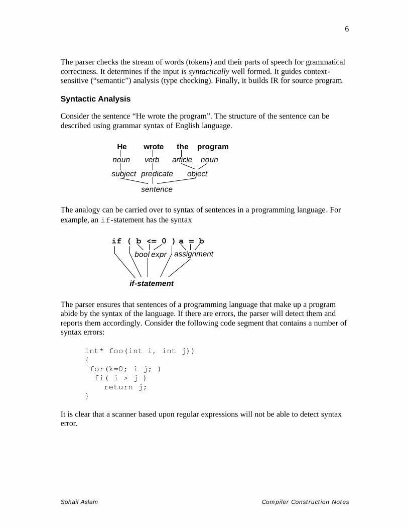
The parser checks the stream of words (tokens) and their parts of speech for grammatical correctness. It determines if the input is syntactically well formed. It guides context-sensitive (“semantic”) analysis (type checking). Finally, it builds IR for source program. Syntactic Analysis
Consider the sentence “He wrote the program”. The structure of the sentence can be described using grammar syntax of English language.
He wrote the program
noun verb article noun
subject predicate object
sentence The analogy can be carried over to syntax of sentences in a programming language. For example, an if-statement has the syntax
if ( b <= 0 ) a = b
bool expr assignment
if-statement The parser ensures that sentences of a programming language that make up a program abide by the syntax of the language. If there are errors, the parser will detect them and reports them accordingly. Consider the following code segment that contains a number of syntax errors:
int* foo(int i, int j)) { for(k=0; i j; ) fi( i > j ) return j; }
It is clear that a scanner based upon regular expressions will not be able to detect syntax error.
LLeeccttuurree 1111
Syntactic Analysis
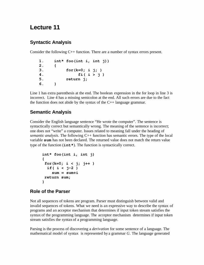
Consider the following C++ function. There are a number of syntax errors present.
1. int* foo(int i, int j)) 2. { 3. for(k=0; i j; ) 4. fi( i > j ) 5. return j; 6. }
Line 1 has extra parenthesis at the end. The boolean expression in the for loop in line 3 is incorrect. Line 4 has a missing semicolon at the end. All such errors are due to the fact the function does not abide by the syntax of the C++ language grammar. Semantic Analysis
Consider the English language sentence “He wrote the computer”. The sentence is syntactically correct but semantically wrong. The meaning of the sentence is incorrect; one does not “write” a computer. Issues related to meaning fall under the heading of semantic analysis. The following C++ function has semantic errors. The type of the local variable sum has not been declared. The returned value does not match the return value type of the function (int*). The function is syntactically correct.
int* foo(int i, int j) { for(k=0; i < j; j++ ) if( i < j-2 ) sum = sum+i return sum; }
Role of the Parser
Not all sequences of tokens are program. Parser must distinguish between valid and invalid sequences of tokens. What we need is an expressive way to describe the syntax of programs and an acceptor mechanism that determines if input token stream satisfies the syntax of the programming language. The acceptor mechanism determines if input token stream satisfies the syntax of a programming language. Parsing is the process of discovering a derivation for some sentence of a language. The mathematical model of syntax is represented by a grammar G. The language generated
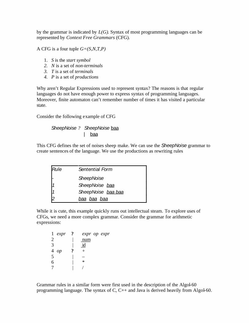
by the grammar is indicated by L(G). Syntax of most programming languages can be represented by Context Free Grammars (CFG). A CFG is a four tuple G=(S,N,T,P)
1. S is the start symbol 2. N is a set of non-terminals 3. T is a set of terminals 4. P is a set of productions
Why aren’t Regular Expressions used to represent syntax? The reasons is that regular languages do not have enough power to express syntax of programming languages. Moreover, finite automaton can’t remember number of times it has visited a particular state. Consider the following example of CFG
SheepNoise ? SheepNoise baa | baa
This CFG defines the set of noises sheep make. We can use the SheepNoise grammar to create sentences of the language. We use the productions as rewriting rules
Rule Sentential Form
- SheepNoise 1 SheepNoise baa 1 SheepNoise baa baa 2 baa baa baa
While it is cute, this example quickly runs out intellectual steam. To explore uses of CFGs, we need a more complex grammar. Consider the grammar for arithmetic expressions:
1 expr ? expr op expr 2 | num 3 | id 4 op ? + 5 | – 6 | * 7 | /
Grammar rules in a similar form were first used in the description of the Algol-60 programming language. The syntax of C, C++ and Java is derived heavily from Algol-60.

The notation was developed by John Backus and adapted by Peter Naur for the Algol-60 language report; thus the term Backus-Naur Form (BNF) Let us use the expression grammar to derive the sentence x – 2 * y
Rule Sentential Form - expr 1 expr op expr 2 <id,x> op expr 5 <id,x> – expr 1 <id,x> – expr op expr 2 <id,x> – <num,2> op expr 6 <id,x> – <num,2> ∗ expr 3 <id,x> – <num,2> ∗ <id,y>
Such a process of rewrites is called a derivation and the process or discovering a derivation is called parsing. At each step, we choose a non-terminal to replace. Different choices can lead to different derivations. Two derivations are of interest
1. Leftmost: replace leftmost non-terminal (NT) at each step 2. Rightmost: replace rightmost NT at each step
The example on the preceding slides was leftmost derivation. There is also a rightmost derivation. In both cases we have expr ? * id – num ∗ id The two derivations produce different parse trees. The parse trees imply different evaluation orders!

LLeeccttuurree 1122
Parse Trees
The derivations can be represented in a tree-like fashion. The interior nodes contain the non-terminals used during the derivation
Precedence
These two derivations point out a problem with the grammar. It has no notion of precedence, or implied order of evaluation. The normal arithmetic rules say that multiplication has higher precedence than subtraction. To add precedence, create a non-
G
E
E op E
E op E x –
2 * y
Leftmost derivation
evaluation order x – ( 2 * y )
G
E
op E
x –
E
E op E
2
* y
Rightmost derivation
evaluation order (x – 2 ) * y

terminal for each level of precedence. Isolate corresponding part of grammar to force parser to recognize high precedence sub-expressions first. Here is the revised grammar: This grammar is larger and requires more rewriting to reach some of the terminal symbols. But it encodes expected precedence. Let’s see how it parses
x – 2 * y
Rule Sentential Form - Goal 1 Expr 3 expr – term 5 expr – term ∗ factor 9 expr – term ∗ <id,y> 7 expr – factor ∗ <id,y> 8 expr – <num,2> ∗ <id,y> 4 term – <num,2> ∗ <id,y> 7 factor – <num,2> ∗ <id,y> 9 <id,x> – <num,2> ∗ <id,y>
This produces same parse tree under leftmost and rightmost derivations
Id | 9
number ? factor 8
factor | 7
term / factor | 6
term ∗ factor ? term 5
term | 4
expr – term | 3
expr + term ? expr 2
expr ? Goal 1
level two
level one

Both leftmost and rightmost derivations give the same expression because the grammar directly encodes the desired precedence. Ambiguous Grammars
If a grammar has more than one leftmost derivation for a single sentential form, the grammar is ambiguous. The leftmost and rightmost derivations for a sentential form may differ, even in an unambiguous grammar. Let’s consider the classic if-then-else example
Stmt ? if Expr then Stmt | if Expr then Stmt else Stmt | … other stmts ….
The following sentential form has two derivations:
if E1 then if E2 then S else S2
G
E
F
T
T F
<id,x>
-–
*
<id,y>
T
E
T
<num,2>
evaluation order x – ( 2 * y )

The convention in most programming languages is to match the else with the most recent if.
Production 1, then Production 2: if E1 then if E2 then S1
else S2
E1
if
then
if
then
else
S1
S2
E2
E1
if
then
if
then else
S1 S2
E2
Production 2, then Production 1: if E1 then if E2 then S1
else S2

We can rewrite grammar to avoid generating the problem and match each else to innermost unmatched if:
1. Stmt
?
If E then Stmt
2. | If E then WithElse else Stmt 3. | Assignment 4. WithElse ? If E then WithElse else WithElse 5. | Assignment
Let derive the following using the rewritten grammar:
if E1 then if E2 then A1 else A2
Context-Free Grammars
We have been using the term context- free without explaining why such rules are in fact “free of context”. The simple reason is that non-terminals appear by themselves to the left of the arrow in context-free rules: A ? α The rule A ? α says that A may be replaced by α anywhere, regardless of where A occurs. On the other hand, we could define a context as pair of strings β , γ , such that a rule would apply only if β occurs before and γ occurs after the non-terminal A. We would write this as β A γ ? β α γ
This binds the else controlling A2 to inner if
E1
Stmt
then
else
A1 A2 E2
if Expr Stmt
Stmt then if Expr Withelse

Such a rule in which α ? ε is called a context-sensitive grammar rule. We would write this as β A γ ? β α γ Such a rule in which α ? ε is called a context-sensitive grammar rule Parsing Techniques
There are two primary parsing techniques: top-down and bottom-up. Top-down parsers
A top-down parsers starts at the root of the parse tree and grows towards leaves. At each node, the parser picks a production and tries to match the input. However, the parser may pick the wrong production in which case it will need to backtrack. Some grammars are backtrack-free. Bottom-up parsers
A bottom-up parser starts at the leaves and grows toward root of the parse tree. As input is consumed, the parser encodes possibilities in an internal state. The bottom-up parser starts in a state valid for legal first tokens. Bottom-up parsers handle a large class of grammars
LLeeccttuurree 1133
Top-Down Parser
A top-down parser starts with the root of the parse tree. The root node is labeled with the goal (start) symbol of the grammar. The top-down parsing algorithm proceeds as follows:
1. Construct the root node of the parse tree 2. Repeat until the fringe of the parse tree matches input string
a. At a node labeled A, select a production with A on its lhs b. for each symbol on its rhs, construct the appropriate child c. When a terminal symbol is added to the fringe and it does not match the
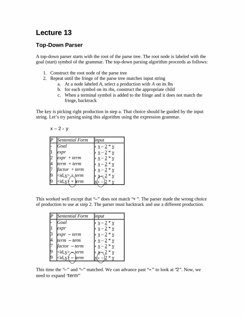
fringe, backtrack The key is picking right production in step a. That choice should be guided by the input string. Let’s try parsing using this algorithm using the expression grammar. x – 2 * y
P Sentential Form input - Goal ↑x – 2 * y 1 expr ↑x – 2 * y 2 expr + term ↑x – 2 * y 4 term + term ↑x – 2 * y 7 factor + term ↑x – 2 * y 9 <id,x> + term ↑x – 2 * y 9 <id,x> + term x ↑– 2 * y
This worked well except that “–” does not match “+”. The parser made the wrong choice of production to use at step 2. The parser must backtrack and use a different production.
This time the “–” and “–” matched. We can advance past “–” to look at “2”. Now, we need to expand “term”
P Sentential Form input - Goal ↑x – 2 * y 1 expr ↑x – 2 * y 3 expr – term ↑x – 2 * y 4 term – term ↑x – 2 * y 7 factor – term ↑x – 2 * y 9 <id,x> – term ↑x – 2 * y 9 <id,x> – term x ↑– 2 * y

The 2’s match but the expansion terminated too soon because there is still unconsumed input and there are no non-terminals to expand in the sentential form ⇒ Need to backtrack.
P Sentential Form input - <id,x> – term x – ↑2 * y 5 <id,x> – term * factor x – ↑2 * y 7 <id,x> – factor * factor x – ↑2 * y 8 <id,x> – <num,2> * factor x – ↑2 * y - <id,x> – <num,2> * factor x – 2 ↑ * y - <id,x> – <num,2> * factor x – 2 * ↑ y 9 <id,x> – <num,2> * <id,y> x – 2 * ↑ y - <id,x> – <num,2> * <id,y> x – 2 * y ↑
This time the parser met with success. All of the input matched. Left Recursion
Consider another possible parse: Parser is using productions but no input is being consumed.
x – 2 ↑* y <id,x> – <num,2> -
x – ↑2 * y <id,x> – <num,2> 9
x – ↑2 * y <id,x> – factor 7
x – ↑2 * y <id,x> – term -
Sentential Form input P
↑x – 2 * y expr +term +term +term +.... 2
↑x – 2 * y expr +term +term +term 2
↑x – 2 * y expr +term +term 2
expr +term
expr
Goal
Sentential Form
↑x – 2 * y 2
↑x – 2 * y 1
↑x – 2 * y -
input P

Top-down parsers cannot handle left-recursive grammars. Formally, a grammar is left recursive if ∃ A ∈ NT such that ∃ a derivation A ⇒* A α , for some string α ∈ (NT ∪ T)*. Our expression grammar is left recursive. This can lead to non-termination in a top-down parser. Non-termination is bad in any part of a compiler! For a top-down parser, any recursion must be a right recursion. We would like to convert left recursion to right To remove left recursion, we can transform the grammar. Consider a grammar fragment: A ? A α | β where neither α nor β starts with A . We can rewrite this as: A ? β A' A' ? α A' | ε where A' is a new non-terminal. This grammar accepts the same language but uses only right recursion. The expression grammar we have been using contains two cases of left- recursion. Applying the transformation yields
expr ? term expr' expr' ? + term expr' | – term expr' term ? factor term' term' ? * factor term' | / factor term' | ε
These fragments use only right recursion. They retain the original left associativity. A top-down parser will terminate using them.

Predictive Parsing
If a top down parser picks the wrong production, it may need to backtrack. Alternative is to look-ahead in input and use context to pick the production to use correctly. How much look-ahead is needed? In general, an arbitrarily large amount of look-ahead symbols are required.. Fortunately, large classes of CFGs can be parsed with limited lookahead. Most programming languages constructs fall in those subclasses The basic idea in predictive parsing is: given A ? α | β , the parser should be able to choose between α and β . To accomplish this, the parser needs FIRST and FOLLOW sets. Definition: FIRST sets: for some rhs α ∈ G, define FIRST(α ) as the set of tokens that appear as the first symbol in some string that derives from α . That is, x ∈ FIRST(α ) iff α ⇒∗ x γ, for some γ .

LLeeccttuurree 1144
The LL(1) Property If A ? α and A ? β both appear in the grammar, we would like
FIRST(α ) ∩ FIRST(β) = ∅
Predictive parsers accept LL(k) grammars. The two LL stand for Left-to-right scan of input, left-most derivation. The k stands for number of look-ahead tokens of input. The LL(1) Property allows the parser to make a correct choice with a look-ahead of exactly one symbol! What about ε-productions? They complicate the definition of LL(1). If A ? α and A ? β and ε ∈ FIRST(α) , then we need to ensure that FIRST(β ) is disjoint from FOLLOW(α ), too. Definition: FOLLOW(α) is the set of all words in the grammar that can legally appear after an α. For a non-terminal X, FOLLOW(X ) is the set of symbols that might follow the derivation of X. Define FIRST+(α) as FIRST(α) ∪ FOLLOW(α), if ε ∈ FIRST(α), FIRST(α), otherwise. Then a grammar is LL(1) iff A ? α and A ? β implies FIRST+(α ) ∩ FIRST+(β) = ∅ Given a grammar that has the is LL(1) property, we can write a simple routine to recognize each lhs. The code is simple and fast. Consider A ? β1 | β2 | β3 , which satisfies the LL(1) property FIRST+(α )∩FIRST+(β) = ∅
/* find an A */ if(token ∈ FIRST(β1)) find a β1 and return true else if(token ∈ FIRST(β 2)) find a β2 and return true if(token ∈ FIRST(β3)) find a β3 and return true else error and return false
Grammar with the LL(1) property are called predictive grammars because the parser can “predict” the correct expansion at each point in the parse. Parsers that capitalize on the LL(1) property are called predictive parsers. One kind of predictive parser is the recursive descent parser.
Recursive Descent Parsing
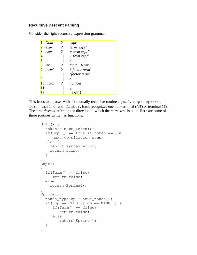
Consider the right-recursive expression grammar
1 Goal ? expr 2 expr ? term expr' 3 expr' ? + term expr' 4 | - term expr' 5 | ε 6 term ? factor term' 7 term' ? * factor term' 8 | / factor term' 9 | ε 10 factor ? number 11 | id 12 | ( expr )
This leads to a parser with six mutually recursive routines: goal, expr, eprime, term, tprime and factor. Each recognizes one non-terminal (NT) or terminal (T). The term descent refers to the direction in which the parse tree is built. Here are some of these routines written as functions:
Goal() { token = next_token(); if(Expr() == true && token == EOF) next compilation step else { report syntax error; return false; } } Expr() { if(Term() == false) return false; else return Eprime(); } Eprime() { token_type op = next_token(); if( op == PLUS || op == MINUS ) { if(Term() == false) return false; else return Eprime(); } }

Functions for other non-terminals Term, Factor and Tprime follow the same pattern. Recursive Descent in C++
This form of the routines is too procedural. Moreover, there is no convenient way to build the parse tree. We can use C++ to code the recursive descent parser in an object oriented manner. We associate a C++ class with each non-terminal symbol. An instantiated object of a non-terminal class contains pointer to the parse tree. Here are the C++ code for the non-terminal classes: class NonTerminal { public:
NonTerminal(Scanner* sc) { s = sc; tree = NULL; } virtual ~NonTerminal(){} virtual bool isPresent()=0; TreeNode* AST(){ return tree; }
protected: Scanner* s; TreeNode* tree; } class Expr:public NonTerminal { public: Expr(Scanner* sc): NonTerminal(sc){ } virtual bool isPresent(); } class Eprime:public NonTerminal { public: Eprime(Scanner* sc, TreeNode* t): NonTerminal(sc) { exprSofar = t; } virtual bool isPresent(); protected: TreeNode* exprSofar; }

class Term:public NonTerminal { public: Term(Scanner* sc): NonTerminal(sc){ } virtual bool isPresent(); } class Tprime:public NonTerminal { public: Tprime(Scanner* sc, TreeNode* t): NonTerminal(sc) { exprSofar = t; } virtual bool isPresent(); protected: TreeNode* exprSofar; } class Factor:public NonTerminal { public: Factor(Scanner* sc, TreeNode* t): NonTerminal(sc){ }; virtual bool isPresent(); }

LLeeccttuurree 1155
Let’s consider the implementation of the C++ classes for the non-terminals. We start with Expr. bool Expr::isPresent() {
Term* op1 = new Term(s); if(!op1->isPresent()) return false; tree = op1->AST(); Eprime* op2 = new Eprime(s, tree); if(op2->isPresent()) tree = op2->AST(); return true;
} bool Eprime::isPresent() { int op=s->nextToken(); if(op==PLUS || op==MINUS){ s->advance(); Term* op2=new Term(s); if(!op2->isPresent()) syntaxError(s); TreeNode* t2=op2->AST(); tree = new TreeNode(op,exprSofar,t2); Eprime* op3 = new Eprime(s, tree); if(op3->isPresent()) tree = op3->AST(); return true; } else return false; } bool Term::isPresent() { Factor* op1 = new Factor(s); if(!op1->isPresent()) return false; tree = op1->AST(); Tprime* op2 = new Tprime(s, tree); if(op2->isPresent()) tree = op2->AST(); return true; }

bool Tprime::isPresent() { int op=s->nextToken(); if(op == MUL || op == DIV){ s->advance(); Factor* op2=new Factor(s); if(!op2->isPresent()) syntaxError(s); TreeNode* t2=op2->AST(); tree = new TreeNode(op,exprSofar,t2); Tprime* op3 = new Tprime(s, tree); if(op3->isPresent()) tree = op3->AST(); return true; } else return false; } bool Factor::isPresent() { int op=s->nextToken(); if(op == ID || op == NUM) { tree = new TreeNode(op,s->tokenValue()); s->advance(); return true; } if( op == LPAREN ){ s->advance(); Expr* opr = new Expr(s); if(!opr->isPresent() ) syntaxError(s); if(s->nextToken() != RPAREN) syntaxError(s); s->advance(); tree = opr->AST(); return true; } return false; }
LLeeccttuurree 1166
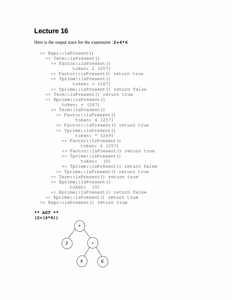
Here is the output trace for the expression : 2+4*6 >> Expr::isPresent() >> Term::isPresent() >> Factor::isPresent() token: 2 (257) << Factor::isPresent() return true >> Tprime::isPresent() token: + (267) << Tprime::isPresent() return false << Term::isPresent() return true >> Eprime::isPresent() token: + (267) >> Term::isPresent() >> Factor::isPresent() token: 4 (257) << Factor::isPresent() return true >> Tprime::isPresent() token: * (269) >> Factor::isPresent() token: 6 (257) << Factor::isPresent() return true >> Tprime::isPresent() token: (0) << Tprime::isPresent() return false << Tprime::isPresent() return true << Term::isPresent() return true >> Eprime::isPresent() token: (0) << Eprime::isPresent() return false << Eprime::isPresent() return true << Expr::isPresent() return true ** AST ** (2+(4*6))
4 6
* 2
+

Non-recursive Predictive Parsing
It is possible to build a non-recursive predictive parser. This is done by maintaining an explicit stack and using a table. Such a parser is called a table-driven parser. The non-recursive LL(1) parser looks up the production to apply by looking up a parsing table. The LL(1) table has one dimension for current non-terminal to expand and another dimension for next token. Each table cell contains one production.
Consider the expression grammar
1 E ? T E' 2 E' ? + T E' 3 | ε 4 T ? F T' 5 T' ? * F T' 6 | ε 7 F ? ( E ) 8 | id
Using the table construction algorithm that will be discussed later, we have the predictive parsing table
id + * ( ) $ E E ? TE' E ? TE' E' E' ? +TE' E' ? ε E' ? ε
T T ? FT' T ? FT' T' T' ? ε T ? *FT' T' ? ε T' ? ε F F ? id F ? (E )
The rows are non-terminals and the columns are the terminals of the expression grammar. The predictive parser uses an explicit stack to keep track of pending non-terminals. It can thus be implemented without recursion.
a + b $
Predictive parser
stack
X Y
Z $
Parsing table M
input
output
LL(1) Parsing Algorithm
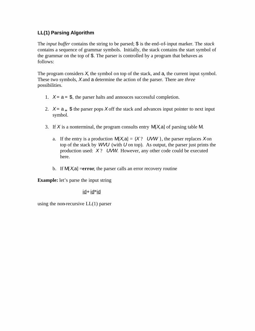
The input buffer contains the string to be parsed; $ is the end-of- input marker. The stack contains a sequence of grammar symbols. Initially, the stack contains the start symbol of the grammar on the top of $. The parser is controlled by a program that behaves as follows: The program considers X, the symbol on top of the stack, and a, the current input symbol. These two symbols, X and a determine the action of the parser. There are three possibilities.
1. X = a = $, the parser halts and annouces successful completion.
2. X = a ≠ $ the parser pops X off the stack and advances input pointer to next input symbol.
3. If X is a nonterminal, the program consults entry M[X,a] of parsing table M. a. If the entry is a production M[X,a] = {X ? UVW }, the parser replaces X on
top of the stack by WVU (with U on top). As output, the parser just prints the production used: X ? UVW. However, any other code could be executed here.
b. If M[X,a] =error, the parser calls an error recovery routine Example: let’s parse the input string id+id∗id using the non-recursive LL(1) parser
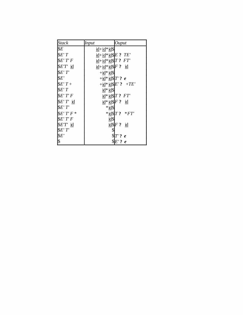
Stack Input Ouput $E id+id∗id$ $E' T id+id∗id$ E ? TE' $E' T' F id+id∗id$ T ? FT' $E'T' id id+id∗id$ F ? id $E' T' +id∗ id$ $E' +id∗ id$ T' ? ε $E' T + +id∗ id$ E' ? +TE' $E' T id∗ id$ $E' T' F id∗ id$ T ? FT' $E' T' id id∗ id$ F ? id $E' T' ∗id$ $E' T' F ∗ ∗id$ T ? ∗FT' $E' T' F id$ $E'T' id id$ F ? id $E' T' $ $E' $ T' ? ε $ $ E' ? ε

LLeeccttuurree 1177
Note that productions output are tracing out a lefmost derivation. The grammar symbols on the stack make up left-sentential forms. LL(1) Table Construction
Top-down parsing expands a parse tree from the start symbol to the leaves. It always expand the leftmost non-terminal. Consider the state S ? ∗ βAγ with b the next token and we are trying to match βbγ. There are two possibilities
1. b belongs to an expansion of A. Any A ? α can be used if b can start a string derived from α. In this case we say that b ∈ FIRST(α )
2. b does not belong to an expansion of A . Expansion of A is empty, i.e., A ? ε and b belongs an expansion of γ , e.g., bω. which means that b can appear after A in a derivation of the form S ? ∗ βAbω. We say that b ∈ FOLLOW(A).
Any A ? α can be used if α expands to ε. We say that ε ∈ FIRST(A) in this case. Definition FIRST(X) = { b | X ? ∗ ba } ∪ { ε | X ? ∗ ε }

LLeeccttuurree 1188
Computing FIRST Sets
Here is the algorithm for computing the FIRST sets. 1. For all terminal symbols b, FIRST(b) = {b} 2. For all productions: X ? A1... An
Add FIRST(A 1) − {ε} to FIRST(X), stop if ε ∉FIRST(A1) Add FIRST(A 2) − {ε} to FIRST(X), stop if ε ∉FIRST(A2) ..... Add FIRST(A n) − {ε} to FIRST(X), stop if ε ∉FIRST(A n) Add ε to FIRST(X)
This strategy is encoded in the following procedure
for each a ∈ ( T ∪ ε ) FIRST(a) ? {a} for each A ∈ NT FIRST(A) ? Ø while ( FIRST sets are still changing) for each A ? β1 β2... βk ∈ P FIRST(A) ? FIRST(A) ∪ (FIRST(β1) – {ε}) i ? 1 while ( ε ∈ FIRST(β i) and i = k-1 ) FIRST(A) ? FIRST(A) ∪ (FIRST(β i+1) – {ε}) i ? i+1 if (i == k and ε ∈ FIRST (βk) FIRST(A) ? FIRST(A) ∪ {ε}
Example : consider the expression grammar again
1 E ? T E' 2 E' ? + T E' 3 | ε 4 T ? F T' 5 T' ? * F T' 6 | ε 7 F ? ( E ) 8 | Id
FIRST(id) = { id } FIRST('(' ) = { ( } FIRST(‘+' ) = { + }
FIRST(E ) = {FIRST(T ) − {ε} } FIRST(T ) = {FIRST(F ) − {ε} } FIRST(F ) = {FIRST( '(') − {ε} } = { ( }
FIRST(F ) = { '(' } + {FIRST( id ) − {ε} } = { ( , id} FIRST(E' ) = { +, ε } FIRST(T' ) = { ∗, ε }
Thus,
FIRST(E ) = FIRST(T ) = FIRST(F ) = { (, id } FIRST(E' ) = { +, ε } FIRST(T' ) = { ∗, ε }
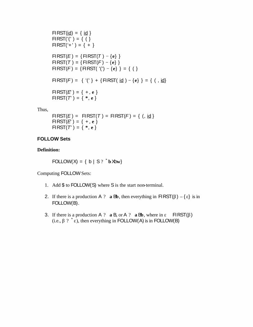
FOLLOW Sets
Definition:
FOLLOW(X) = { b | S ? ∗ βXbω} Computing FOLLOW Sets:
1. Add $ to FOLLOW(S) where S is the start non-terminal.
2. If there is a production A ? αBβ , then everything in FIRST(β) – {ε} is in FOLLOW(B).
3. If there is a production A ? αB, or A ? αBβ , where in ε ∈ FIRST(β) (i.e., β ? ∗ ε), then everything in FOLLOW(A) is in FOLLOW(B)

The following procedure encodes this strategy. for each A ∈ NT FOLLOW(A) ? Ø FOLLOW(S) ? {$} while ( FOLLOW sets are still changing) for each A ? β1 β2... βk ∈ P FOLLOW(βk) ? FOLLOW(βk) ∪ FOLLOW(A) T ? FOLLOW(A) for i ? k downto 2 if ( ε ∈ FIRST (β i) ) FOLLOW(β i-1) ? FOLLOW(β i-1) ∪ (FIRST(β i) – {ε}) ∪ T else FOLLOW(β i-1) ? FOLLOW(β i-1) ∪FIRST(β i) T ? Ø Let’s apply the algorithm to the expression grammar. Put $ in FOLLOW(E ). By rule (2) applied to production ? ( E ), ‘)’ is also in FOLLOW(E ). Thus, FOLLOW(E ) = { ), $}. By rule (3) applied to production E ? T E' , $ and ‘)’ are in FOLLOW(E' ). Thus, FOLLOW(E ) = FOLLOW (E' ) = { ), $ }. Similarly, FOLLOW(T ) = FOLLOW (T' ) = { +, ), $ } and FOLLOW(F ) = { +, ∗, ), $ }
Sohail Aslam Compiler Construction Notes Set:2-1
LLeeccttuurree 1199
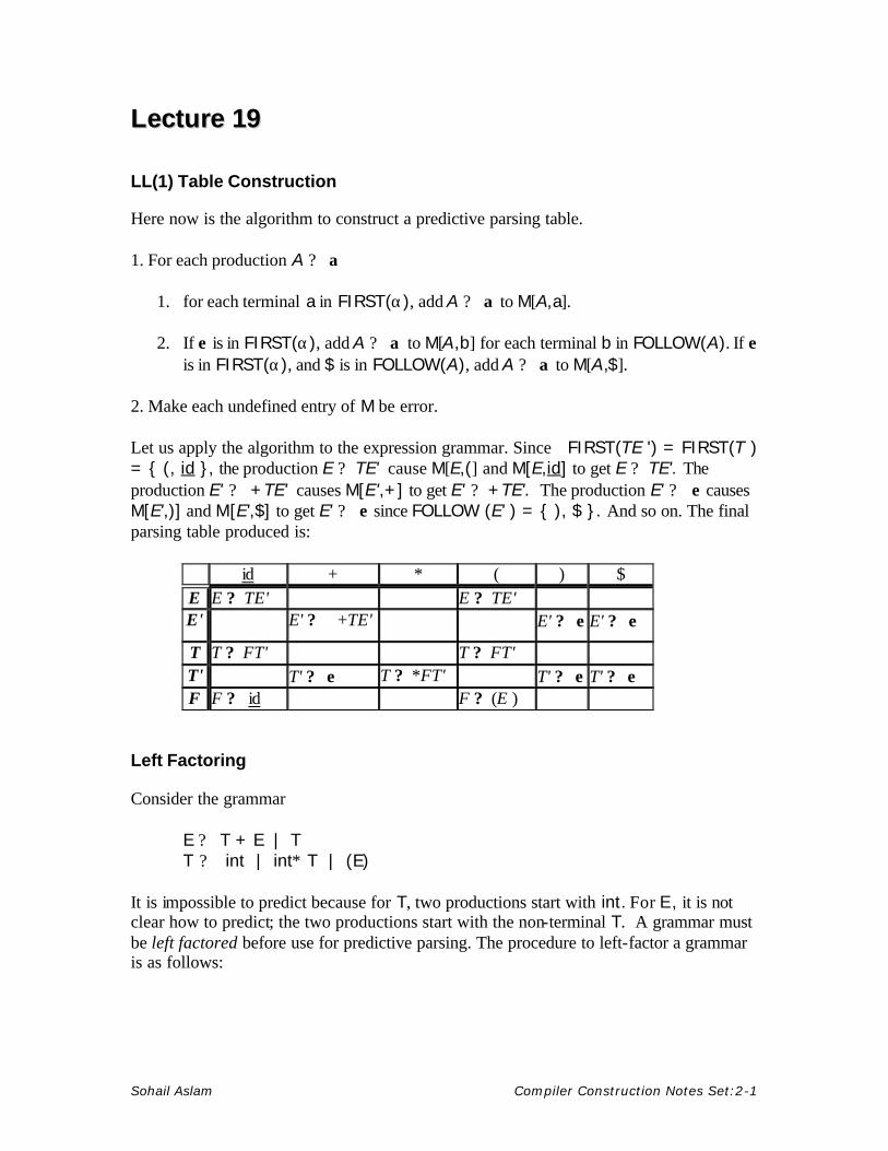
LL(1) Table Construction
Here now is the algorithm to construct a predictive parsing table. 1. For each production A ? α
1. for each terminal a in FIRST(α), add A ? α to M[A,a].
2. If ε is in FIRST(α), add A ? α to M[A,b] for each terminal b in FOLLOW(A). If ε is in FIRST(α), and $ is in FOLLOW(A), add A ? α to M[A,$].
2. Make each undefined entry of M be error. Let us apply the algorithm to the expression grammar. Since FIRST(TE ') = FIRST(T ) = { (, id }, the production E ? TE' cause M[E,(] and M[E,id] to get E ? TE'. The production E' ? +TE' causes M[E',+] to get E' ? +TE'. The production E' ? ε causes M[E',)] and M[E',$] to get E' ? ε since FOLLOW (E' ) = { ), $ }. And so on. The final parsing table produced is:
id + * ( ) $ E E ? TE' E ? TE' E' E' ? +TE' E' ? ε E' ? ε
T T ? FT' T ? FT' T' T' ? ε T ? *FT' T' ? ε T' ? ε F F ? id F ? (E )
Left Factoring
Consider the grammar
E ? T + E | T T ? int | int∗ T | (E)
It is impossible to predict because for T, two productions start with int. For E, it is not clear how to predict; the two productions start with the non-terminal T. A grammar must be left factored before use for predictive parsing. The procedure to left-factor a grammar is as follows:
Sohail Aslam Compiler Construction Notes Set:2-2
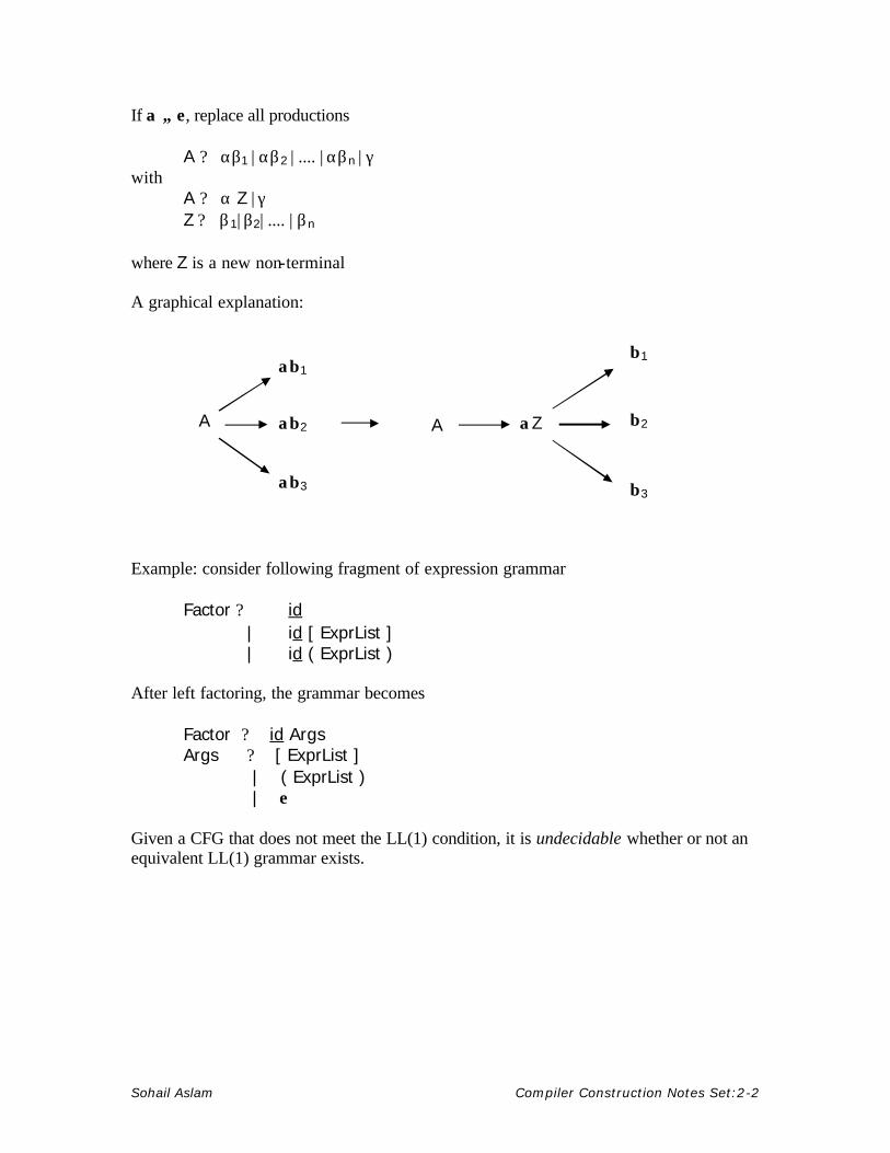
If α ≠ ε, replace all productions A ? αβ1 | αβ2 | .... | αβn | γ with A ? α Z | γ Z ? β1| β2| .... | βn
where Z is a new non-terminal A graphical explanation:
Example: consider following fragment of expression grammar
Factor ? id | id [ ExprList ] | id ( ExprList ) After left factoring, the grammar becomes Factor ? id Args Args ? [ ExprList ] | ( ExprList ) | ε Given a CFG that does not meet the LL(1) condition, it is undecidable whether or not an equivalent LL(1) grammar exists.
A αβ2
αβ1
αβ3
β2
β1
β3
αZ A

Sohail Aslam Compiler Construction Notes Set:3-63
63
LLeeccttuurree 2200 Bottom-up Parsing
Bottom-up parsing is more general than top-down parsing. Bottom-up parsers handle a large class of grammars. It is the preferred method in practice. It is also called LR parsing; L means that tokens are read left to right and R means that the parser constructs a rightmost derivation. LR parsers do not need left-factored grammars. LR parsers can handle left-recursive grammars. LR parsing reduces a string to the start symbol by inverting productions.A derivation consists of a series of rewrite steps S ⇒ γ0 ⇒ γ1 ⇒ ... ⇒ γn-1 ⇒ γn ⇒ sentence Each γi is a sentential form. If γ contains only terminals, γ is a sentence in L(G). If γ contains ≥ 1 nonterminals, γ is a sentential form. A bottom-up parser builds a derivation by working from input sentence back towards the start symbol S. Consider the grammar S → aABe A → Abc | b B → d The sentence abbcde can be reduced to S: abbcde aAbcde aAde aABe S These reductions, in fact, trace out the following right-most derivation in reverse: S ⇒ aABe ⇒ aAde ⇒ aAbcde ⇒ abbcde S ⇒ aBy ⇒ aγy ⇒ xy

Sohail Aslam Compiler Construction Notes Set:3-64
64
Consider the grammar 1. E → E + (E) 2. | int The bottom-up parse of the string int + (int) + (int) would be
int + (int) + (int) E + (int) + (int) E + (E) + (int) E + (int) E + (E) E
The consequence of an LR parser tracing a rightmost derivation in reverse is that given αβγ be a step of a bottom-up parse, assuming that next reduction is A → β τhen γ is a string of terminals. The reason is that αAγ → αβγ is a step in a rightmost derivation. This observation provides a strategy for building bottom up parsers: split the input string into two substrings. Right substring (a string of terminals) is as yet unexamined by parser and left substring has terminals and non-terminals. The dividing point is marked by a ► (the ► is not part of the string). Initially, all input is unexamined: ►x1 x1 . . . xn. Shift-Reduce Parsing
Bottom-up parsing uses only two kinds of actions: 1. Shift 2. Reduce
α
x y
B
S
γ
rule: B → γ
Terminals only
Sohail Aslam Compiler Construction Notes Set:3-65
65
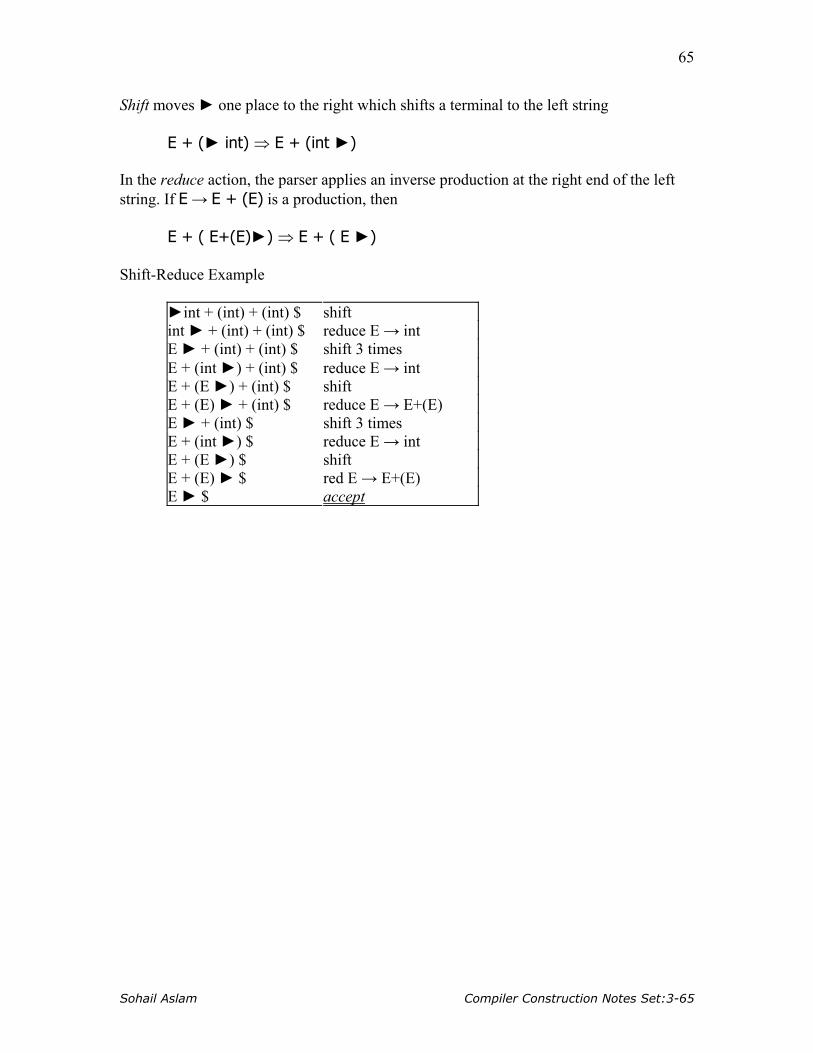
Shift moves ► one place to the right which shifts a terminal to the left string E + (► int) ⇒ E + (int ►) In the reduce action, the parser applies an inverse production at the right end of the left string. If E → E + (E) is a production, then E + ( E+(E)►) ⇒ E + ( E ►) Shift-Reduce Example
►int + (int) + (int) $ shift int ► + (int) + (int) $ reduce E → int E ► + (int) + (int) $ shift 3 times E + (int ►) + (int) $ reduce E → int E + (E ►) + (int) $ shift E + (E) ► + (int) $ reduce E → E+(E) E ► + (int) $ shift 3 times E + (int ►) $ reduce E → int E + (E ►) $ shift E + (E) ► $ red E → E+(E) E ► $ accept

Sohail Aslam Compiler Construction Notes Set:3-65
65
LLeeccttuurree 2211 Shift-Reduce: The Stack
A stack can be used to hold the content of the left string. The Top of the stack is marked by the ► symbol. The shift action pushes a terminal on the stack. Reduce pops zero or more symbols from the stack (production rhs) and pushes a non-terminal on the stack (production lhs) Discovering Handles
A bottom-up parser builds the parse tree starting with its leaves and working toward its root. The upper edge of this partially constructed parse tree is called its upper frontier. At each step, the parser looks for a section of the upper frontier that matches right-hand side of some production. When it finds a match, the parser builds a new tree node with the production’s left-hand non-terminal thus extending the frontier upwards towards the root. The critical step is developing an efficient mechanism that finds matches along the tree’s current frontier. Formally, the parser must find some substring β, of the upper frontier where
1. β is the right-hand side of some production A → β, and 2. A → β is one step in right-most derivation of input stream
We can represent each potential match as a pair ⟨A→β,k⟩, where k is the position on the tree’s current frontier of the right-end of β. The pair ⟨A→β,k⟩, is called the handle of the bottom-up parse. Handle Pruning
A bottom-up parser operates by repeatedly locating handles on the frontier of the partial parse tree and performing reductions that they specify. The bottom-up parser uses a stack to hold the frontier. The stack simplifies the parsing algorithm in two ways. First, the stack trivializes the problem of managing space for the frontier. To extend the frontier, the parser simply pushes the current input token onto the top of the stack. Second, the stack ensures that all handles occur with their right end at the top of the stack. This eliminates the need to represent handle’s position.

Sohail Aslam Compiler Construction Notes Set:3-66
66
Shift-Reduce Parsing Algorithm
push $ onto stack sym ← nextToken() repeat until (sym == $ and the stack contains exactly Goal on top of $) if a handle for A → β on top of stack pop |β| symbols off the stack push A onto the stack else if (sym ≠ $ ) push sym onto stack sym ← nextToken() else /* no handle, no input */ report error and halt

Sohail Aslam Compiler Construction Notes Set:3-67
67
LLeeccttuurree 2222 Example: here is the bottom-up parser’s action when it parses the expression grammar sentence x – 2 × y (tokenized as id – num * id) word Stack Handle Action 1 id ► - none - shift 2 – id ► ⟨Factor → id,1⟩ reduce 3 – Factor ► ⟨Term → Factor,1⟩ reduce 4 – Term ► ⟨Expr → Term,1⟩ reduce 5 – Expr ► - none - shift 6 num Expr – ► - none - shift 7 × Expr – num ► ⟨Factor → num,3⟩ reduce 8 × Expr – Factor ► ⟨Term → Factor,3⟩ shift 9 × Expr – Term ► - none - shift 10 id Expr – Term × ► - none - shift 11 $ Expr – Term × id► ⟨Factor → id,5⟩ reduce 12 $ Expr–Term × Factor► ⟨Term→Term×Factor,5⟩ reduce 13 $ Expr – Term ► ⟨Expr → Expr – Term,3⟩ reduce 14 $ Expr ► ⟨Goal → Expr,1⟩ reduce 15 $ Goal - none - accept Handles
The handle-finding mechanism is the key to efficient bottom-up parsing. As it process an input string, the parser must find and track all potential handles. For example, every legal input eventually reduces the entire frontier to grammar’s goal symbol. Thus, ⟨Goal → Expr,1⟩ is a potential handle at the start of every parse. As the parser builds a derivation, it discovers other handles. At each step, the set of potential handles represent different suffixes that lead to a reduction. Each potential handle represent a string of grammar symbols that, if seen, would complete the right-hand side of some production.

Sohail Aslam Compiler Construction Notes Set:3-68
68
For the bottom-up parse of the expression grammar string, we can represent the potential handles that the shift-reduce parser should track. Using the placeholder • to represent top of the stack, there are nine handles:
Handles 1 ⟨Factor → id •⟩ 2 ⟨Term → Factor•⟩ 3 ⟨Expr → Term •⟩ 4 ⟨Factor → num•⟩ 5 ⟨Term → Factor•⟩ 6 ⟨Factor → id •⟩ 7 ⟨Term → Term × Factor •⟩ 8 ⟨Expr → Expr – Term •⟩ 9 ⟨Goal → Expr •⟩
This notation shows that the second and fifth handles are identical, as are first and sixth. It also create a way to represent the potential of discovering a handle in future. Consider the parser’s state in step 6: The parser has recognized Expr –. Using the stack-relative notation, we can represent the parser’s state as Expr → Expr – • Term. The parser has already recognized an Expr and a –. If the parser reaches a state where it shifts a Term on top of Expr and –, it will complete the handle Expr → Expr – Term •. How many potential handles must the parser recognize? The right-hand side of each production can have a placeholder at its start, at its end and between any two consecutive symbols.
Expr → • Expr –Term Expr → Expr • – Term Expr → Expr – •Term Expr → Expr – Term •
If the right-hand side of a production has k symbols, it has k +1 placeholder positions.
Sohail Aslam Compiler Construction Notes Set:2-1
LLeeccttuurree 2233 Handles
The number of potential handles for the grammar is simply the sum of the lengths of the right-hand side of all the productions. The number of complete handles is simply the number of productions. These two facts lead to the critical insight behind LR parsers:
A given grammar generates a finite set of handles (and potential handles) that the parser must recognize
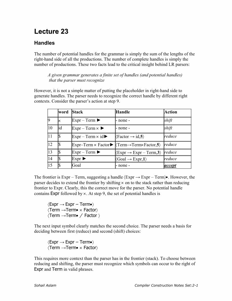
However, it is not a simple matter of putting the placeholder in right-hand side to generate handles. The parser needs to recognize the correct handle by different right contexts. Consider the parser’s action at step 9.
word Stack Handle Action
9 × Expr – Term ► - none - shift
10 id Expr – Term × ► - none - shift
11 $ Expr – Term × id► ⟨Factor → id,5⟩ reduce
12 $ Expr–Term × Factor► ⟨Term→Term×Factor,5⟩ reduce
13 $ Expr – Term ► ⟨Expr → Expr – Term,3⟩ reduce 14 $ Expr ► ⟨Goal → Expr,1⟩ reduce 15 $ Goal - none - accept
The frontier is Expr – Term, suggesting a handle ⟨Expr → Expr – Term⟩•. However, the parser decides to extend the frontier by shifting × on to the stack rather than reducing frontier to Expr. Clearly, this the correct move for the parser. No potential handle contains Expr followed by ×. At step 9, the set of potential handles is ⟨Expr → Expr – Term•⟩ ⟨Term →Term• × Factor⟩ ⟨Term →Term• / Factor ⟩ The next input symbol clearly matches the second choice. The parser needs a basis for deciding between first (reduce) and second (shift) choices: ⟨Expr → Expr – Term•⟩ ⟨Term →Term• × Factor⟩ This requires more context than the parser has in the frontier (stack). To choose between reducing and shifting, the parser must recognize which symbols can occur to the right of Expr and Term in valid phrases.
Sohail Aslam Compiler Construction Notes Set:2-2
LR(1) Parsers
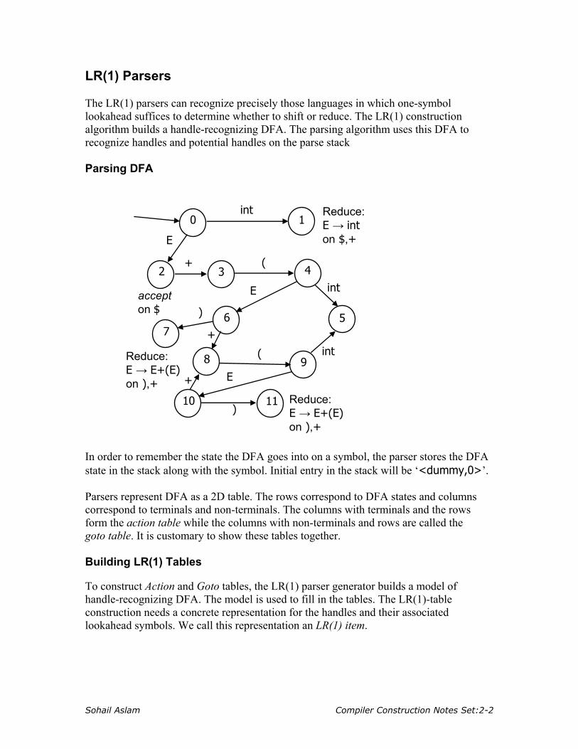
The LR(1) parsers can recognize precisely those languages in which one-symbol lookahead suffices to determine whether to shift or reduce. The LR(1) construction algorithm builds a handle-recognizing DFA. The parsing algorithm uses this DFA to recognize handles and potential handles on the parse stack Parsing DFA
In order to remember the state the DFA goes into on a symbol, the parser stores the DFA state in the stack along with the symbol. Initial entry in the stack will be ‘<dummy,0>’. Parsers represent DFA as a 2D table. The rows correspond to DFA states and columns correspond to terminals and non-terminals. The columns with terminals and the rows form the action table while the columns with non-terminals and rows are called the goto table. It is customary to show these tables together. Building LR(1) Tables
To construct Action and Goto tables, the LR(1) parser generator builds a model of handle-recognizing DFA. The model is used to fill in the tables. The LR(1)-table construction needs a concrete representation for the handles and their associated lookahead symbols. We call this representation an LR(1) item.
0
10
1
2 3 4
7 6 5
11
8 9
int
E
E
+ (
E
)
+
int
int(
+
)
Reduce:E → int on $,+
accept on $
Reduce: E → E+(E) on ),+
Reduce: E → E+(E) on ),+
Sohail Aslam Compiler Construction Notes Set:2-1
1
LLeeccttuurree 2244 An LR(1) item is a pair [X → α•β, a] where X → αβ is a production and a∈T (terminals) is look-ahead symbol. The model uses a set of LR(1) items to represent each parser state. The model is called the canonical collection (CC) of set of LR(1) items. Canonical Collection
Each set in CC represents a state in the eventual parser DFA. The construction of CC begins by building a model of parser’s initial state. The initial state consists of the set of LR(1) items that represent the parser’s initial state, along with any items that must also hold in the initial state. To simplify the task of building this initial state, the construction requires that the grammar have a unique goal symbol. The convention is to add a new start symbol S to grammar and a production S → E This leads to the augmented grammar S → E E → E + (E) | int The Closure Procedure
The item [S → •E, $] describes the parser’s initial state. It represents a configuration in which recognizing S followed by $ would be a valid parse. This item, i.e., [S → •E, $] becomes the core of the first state in CC, labeled I0. If the grammar has several distinct productions for the start symbol, each of them generates an item in this initial core of I0. The procedure closure does this.
closure(s) = repeat for each [X → α•Yβ, a] ∈ s for each production Y → α for each b ∈ FIRST(βa) s ← s ∪ [Y → • γ, b] until s is unchanged
Let’s apply this procedure to the augmented grammar. The first set is I0 = closure({[S → •E, $] }). Equating the terms in the procedure, s = {[S → •E, $]}, [X → α •Yβ, a] ⇔ [S → •E, $], X = S, α = ε, Y = E, β = ε, a = $, Y → γ ⇔E → E + (E) and E → int FIRST(βa) = FIRST($) = $.
Sohail Aslam Compiler Construction Notes Set:2-2
2
This leads to expansion of s. s = { [S → •E, $] } ∪ { [E → •E + (E), $] } ∪ { [E → •int, $] } = { [S → •E, $] , [E → •E + (E), $] , [E → •int, $] } The set s changed so we repeat. The item [S → •E, $] is already processed. The for loop considers [X → α•Yβ, a] ⇔ [E→•E+(E),$], which leads to the match up X = E, α= ε, Y = E, β = +(E), a = $, Y → γ ⇔ E → E + (E), ⇔ E → int FIRST(βa) = FIRST(+(E)$) = +. The set s is extended s = s ∪ { [E → •E+(E), +] } ∪ { [E → •int, +] }

Sohail Aslam Compiler Construction Notes Set:2-1
1
LLeeccttuurree 2255 The set s changed so the repeat loop is executed again. This time, however, the item [E → •int, $/+] does not yield any more items because the dot is followed by the terminal int. The first set of items is I0 = { [S → •E, $], [E → •E+(E), $/+], [E → •int, $/+] } Let’s consider the rationale behind the Closure procedure. If [A → β•Cδ,a] ∈ s, then one potential completion for the left context is to find a string that reduces to C, followed by δa. This completion should cause a reduction to A, since it fills out the production’s right-hand side (Cδ), and follows it with a valid look-ahead symbol. For a production C → γ, closure must insert '•' before γ and add appropriate look-ahead symbols – all terminals that can appear as the initial symbol in δa. This includes every terminal in FIRST(δ). If ε ∈ FIRST(δ), it also includes a, thus FIRST(δa) in the algorithm. The goto Procedure
The second critical step in the construction is to derive other parser states from I0. To accomplish this, we compute, for each state Ii and each grammar symbol y, the state that would arise if the parser recognized a y while in state Ii. A state s that contains [X → α • yβ, b] has a transition (goto) labeled y to the state that contains the items goto(s, y) where y can be terminal or a non-terminal.
goto(s, y) m ← { } for each item [X → α •yβ, b] ∈ s m ← m ∪ {[X → α y•β, b]} return closure(m)
Finite Automaton of Items
The LR(1) items are used as the states of a finite automaton (FA) that maintains information about the parsing stack and progress of a shift-reduce parser. The FA will start out as a nondeterministic finite automaton (NFA). A DFA can be constructed from this NFA using the subset construction, similar to one we used for lexical analysis. Consider the NFA of LR(0) items, i.e., no look-ahead. What are the transitions of the NFA of LR(0) items? Consider the item A→ α•γ. Suppose γ begins with symbol X which may be a terminal (token) or non-terminal. The item can be written as A→ α•Xη.

Sohail Aslam Compiler Construction Notes Set:2-2
2
Then there is a transition on symbol X for state represented by item A→ α•Xη to state represented by item A→ αX•η. If X is a terminal, then this transition corresponds to a shift of X from input to top of parse stack.
If X is a non-terminal, then the interpretation of this transition is more complex because non-terminals do not appear in input. In fact, such a transition will correspond to pushing of X onto the stack during the parse. But this can only occur during a reduction by the production X → β. Such a reduction must be preceded by recognition of a β. The state given by X → •β represents the beginning of this process (dot indicates we are about to recognize β). Then for every item A→ α•Xη we must add an ε-transition for every production X → β.
A → α•Xη
X → • β ε
A → α•Xη A → αX• η X

Sohail Aslam Compiler Construction Notes Set:2-1
1
LLeeccttuurree 2266 The initial DFA state I0 we computed is the ε-closure of the set consisting of item S → •E Recall the stage in the closure s = { [S → •E, $] , [E → •E + (E), $] , [E → •int, $] } The NFA states and transitions required are
Algorithm: Construction of collection of canonical sets of LR(1) items. Input: An augmented grammar G' Output: Collection of canonical (CC) sets of LR(1)
[S → •E,$]
ε
[E → •E+(E),$]
[E → •int,$] ε
Sohail Aslam Compiler Construction Notes Set:2-2
2
CC(G') I0 ← {closure([S' → •S, $])} CC ← { I0 } repeat for each unmarked set Ij ∈ CC mark Ij as processed
for each X following • in an item in Ij Ik ← goto(Ij,X) if Ik ∉ CC then CC ← CC ∪ Ik record transition from Ij to Ik on X until CC is not changing We use the algorithm to compute the sets of LR(1) items for the augmented grammar G'
S → E E → E + (E) | int
We computed I0; we now compute the sets goto(I0,X) for various values of X. X can be E, int, +, ( and ) . I1 = goto(I0,int): invokes closure({[E → int•,$/+]}). No additional closure is possible since the dot is at the right end of the production. Thus I1 = {[E → int•, $/+]} and we have the transition from I0 to I1 on int I2 = goto(I0,E) m ← {} for each [X → �•E�, b] ∈ I0 ⇔[S → •E, $] ⇔[E → •E+(E), $/+] m = m ∪ {[S → E•, $]} ∪ {[E → E•+(E), $/+]} return closure(m) No further closure for the first item because • is at the end In the second item, a terminal + appears after • so no further closure is possible. Thus I2 = {[S → E•, $], [E → E• +(E), $/+]}. We repeat the process in similar fashion. I3 = goto(I2,+) = {[E → E + • (E), $/+]}

Sohail Aslam Compiler Construction Notes Set:2-3
3
I4 = goto(I3,( ) = { [E → E + (• E), $/+], [E → • E + (E), )/+], [E → • int, )/+]} I3 = goto(I2,+) = {[E → E + • (E), $/+]} I4 = goto(I3,( ) = {[E → E + (• E), $/+], [E → • E + (E), )/+], [E → • int, )/+]} I5 = goto(I4, int) = { [E → int •, )/+] } I6 = goto(I4, E ) = { [E → E + (E •), $/+], [E → E • + (E), )/+] } and so on. The sets and transitions so far yield the DFA
0
reduce E → int on ),+
int
E +
(
E
int
reduce: E → int on $,+
accept on $
S→ •E, $ E→ •E+(E), $/+ E→ •int, $/+
1 E→ int •, $/+
2 S→ E•, $ E→ E• +(E), $/+ 3 E→ E+•(E), $/+
4 E→ E+(•E), $/+ E→ •E+(E), )/+ E→ •int, )/+
6 E→ E+(•E), $/+ E→ •E+(E), )/+ E→ •int, )/+
5E→ int •, )/+

Sohail Aslam Compiler Construction Notes Set:2-1
1
LLeeccttuurree 2277 LR Table Construction
Construct CC = {I0,I1,I2, ... , In}, for G'. State i of the parser is constructed from the set Ii The parsing actions for state i are determined as follows: for each item Ii ∈ CC if [A → α•a β, b] ∈ Ii and goto(Ii, a) == Ij then Action[i,a] ← “shift j” else if [A → �•, a] ∈ Ii and A ≠ S' then Action[i,a] ← “reduce A → α ” else if [S' → S•, $] ∈ Ii then Action[i,a] ← “accept” end for // the goto table for each non-terminal A ∈ G if goto(Ii, A) = Ij then Goto[i, A] ← j The initial state is the one that contains the item [S' → •S, $]. All remaining entries are marked “error”. Let us go through an example and construct the LR table for the augmented grammar
1. S' → E 2. E → T – E 3. E → T 4. T → F × T 5. T → F 6. F → id
The FIRST sets we would need are Symbol FIRST S' { id } E { id } T { id } F { id } id { id } × { × } – { – }

Sohail Aslam Compiler Construction Notes Set:2-2
2
We construct the canonical collection of set of LR(1) I0 = {closure([S' → •E, $])} {
[S' → •E, $], [E → •T – E, $], [E → •T, $], [T → •F×T, $], [T → •F, $] [T → •F×T, –], [T → •F, –], [F → •id, $], [F → •id, –], [F → •id, ×]
} I1 = {goto(I0, E)} = {[S' → E•, $] } I2 = {goto(I0, T)} = {[E → T• – E,$], [E →T•,$]} I3 = {goto(I0, F)} = { [T → F• ×T, $], [T → F•, $], [T → F• ×T, –], [T → F•, –] } I4 = {goto(I0, id)} = { [F → id •, $], [F → id •, –], [F → id •, ×] } I5 = {goto(I2, –)} = {
[E →T– • E, $], [E → •T–E, $], [E → •T, $], [T → •F×T, $], [T → •F×T, –], [T → •F, $], [T → •F, –], [F → •id, $], [F → •id, –], [F → •id, ×] }
I6 = {goto(I3, ×)} = {
[T → F× •T, $], [T → F× •T, –], [T → •F×T, $], [T → •F×T, –], [T → •F, $], [T → •F, –], [F → •id, $], [F → •id, –], [F → •id, ×] } I7 = {goto(I5, E)} = {[E → T – E •, $] } I2 = {goto(I5, T)}, i.e., goto(I5, T) yields the same set as I2. I3 = {goto(I5, F)} I4 = {goto(I5, id)}

Sohail Aslam Compiler Construction Notes Set:2-3
3
I8 = {goto(I6, T)} = { [T → F×T •, $], [T → F×T •, –] } I3 = {goto(I6, F)} I4 = {goto(I6, id)} We now filling the LR(1) table by applying the rules. Apply 1. if [A → α•aβ, b] ∈ Ii and goto(Ii, a) = Ij
then set Action[i,a] ← “shift j”. // here, a is a terminal. I0={[S' → •E,$],[E →•T– E, $], [E → •T, $], [T → •F×T, $], [T → •F×T, –], [T → •F, $], [T → •F, –], [F → •id, $], [F → •id, –], [F → •id, ×] } goto(I0, id) = I4 ⇒ Action[0, id] ← shift 4 I2= {[E → T• – E, $], [E →T•,$]}, goto(I2, –) = I5
⇒ Action[2, –] ← shift 5 I3={[T → F• ×T, $], [T → F•, $],[T → F• ×T, –], [T → F•, –]}, goto(I3, ×) = I6
⇒ Action[3, ×] ← shift 6 goto(I5, id) = I4
⇒ Action[5, id] ← shift 4 goto(I6, id) = I4
⇒ Action[6, id] ← shift 4 Apply 2. if [A → α•, a] ∈ Ii and A ≠ S' then set action[i,a] to “reduce A → α” I2 = { [E → T• – E, $], [E →T•,$] }
⇒ Action[2, $] ← reduce 3 I3 = {[T → F• ×T, $], [T → F•, $], [T → F• ×T, –], [T → F•, –] }
⇒ Action[3, $] ← reduce 5 ⇒ Action[3, –] ← reduce 5

Sohail Aslam Compiler Construction Notes Set:2-4
4
I4 = {[F → id•, $], [F → id•, –], [F → id•, ×] }
⇒ Action[4, $] ← reduce 6 ⇒ Action[4, –] ← reduce 6 ⇒ Action[4, ×] ← reduce 6
I7 = {[E → T – E•, $] }
⇒ Action[7, $] ← reduce 2
I8 = { [T → F×T•, $], [T → F×T•, –] } ⇒ Action[8, $] ← reduce 4 ⇒ Action[8, –] ← reduce 4
Apply 3. if [S' → S•, $] ∈ Ii
then set action[i,$] to “accept” I1 = {[S' → E•, $] }
⇒ Action[1, $] ← accept Apply for each non-terminal A ∈ G
if goto(Ii, A) = Ij then goto[i, A] ← j. goto(I0, E) = I1 ⇒ goto[0,E] ← 1 goto(I0, T) = I2 ⇒ goto[0,T] ← 2 goto(I0, F) = I3 ⇒ goto[0,F] ← 3 goto(I5, E) = I7 ⇒ goto[5,E] ← 7 goto(I5, T) = I2 ⇒ goto[5,T] ← 2 goto(I5, F) = I3 ⇒ goto[5,F] ← 3 goto(I6, T) = I8 ⇒ goto[6,T] ← 8 goto(I6, F) = I3 ⇒ goto[6,F] ← 3

Sohail Aslam Compiler Construction Notes Set:2-5
5
The final table we get is
Action Goto id – × $ E T F 0 s4 1 2 3 1 acc 2 s5 r3 3 r5 s6 r5 4 r6 r6 r6 5 s4 7 2 3 6 s4 8 3 7 r2 8 r4 r4
Let us parse the expression x – y × z using the LR(1) table. The scanner will encode the input string as id – id × id $ where $ is the EOF marker
Stack Input ¤0 id – id × id $s4 ¤0id4 – id × id $r6 F→ id ¤0F3 – id × id $r5 T→ F ¤0T2 – id × id $s5 ¤0T2–5 id × id $s4 ¤0T2–5id4 × id $r6 F→ id ¤0T2–5F3 × id $s6 ¤0T2–5F3×6 id $s4 ¤0T2–5F3×6id4 $r6 F→ id ¤0T2–5F3×6F3 $r5 T→ F ¤0T2–5F3×6T8 $r4 T→ F×T ¤0T2–5T2 $r3 E→T ¤0T2 –5E7 $r2 E→T–E ¤0E1 $accept
Sohail Aslam Compiler Construction Notes Set:2-1
1
LLeeccttuurree 2288 LR(1) Skeleton Parser
stack.push(dummy); stack.push(0); done = false; token = scanner.next(); while (!done) { s = stack.top(); if( Action[s,token] == “reduce A→β”) { stack.pop(2×|β|); s = stack.top(); stack.push(A); stack.push(Goto[s,A]); } else if( Action[s,token] == “shift i”){ stack.push(token); stack.push(i); token = scanner.next(); } else if(Action[s,token] == “accept” && token == “$” ) done = true; else report error and recover; } report success; Shift/Reduce Conflicts
If a DFA states contains both [X → α•aβ, b] and [Y → γ•, a] Then on input “a” we could either shift into state [X → αa•β,b], or reduce with Y → γ. This is called a shift-reduce conflict. Typically, this is due to ambiguities in the grammar. The classic example of a shift-reduce conflict is the dangling else. Consider the grammar
stmt → if E then stmt | if E then stmt else stmt We will have DFA state containing [stmt → if E then stmt•, else] [stmt → if E then stmt •else stmt, x] If else follows, we can shift [stmt → if E then stmt else • stmt, x]

Sohail Aslam Compiler Construction Notes Set:2-2
2
or reduce [stmt → if E then stmt•, else] Typical action is shift so that else matches with most recent if.

Sohail Aslam Compiler Construction Notes Set:2-1
1
LLeeccttuurree 2299 Shift/Reduce Conflicts
Consider the ambiguous grammar E → E + E | E × E | int We will DFA state containg [E → E × E•, +] [E → E • + E, +] Again we have a shift/reduce conflict. We need to reduce because × has precedence over + Reduce/Reduce Conflicts
If a DFA states contains both [X → α •, a] and [Y → β •, a], then on input “a” we don’t know which production to reduce with. This is called a reduce-reduce conflict. Usually due to gross ambiguity in the grammar. LR(1) Table Size
LR(1) parsing table for even a simple language can be extremely large with thousands of entries. It is possible to reduce the size of the table. Many states in the DFA are similar. The core of set of LR items is the set of first components without the lookahead terminals. For example the core of the item { [X → α•β, b], [Y → γ•δ, d] } is { X → α•β, Y → γ•δ }. Consider the LR(1) states
{ [X → α •, a], [Y → β •, c] } { [X → α •, b], [Y → β •, d] }
They have the same core and can be merged. The merged state contains { [X → α •, a/b], [Y → β •, c/d]} These are called the LALR(1) states. LALR(1) stands for LookAhead LR(1). This leads to tables that have 10 times fewer states than LR(1).

Sohail Aslam Compiler Construction Notes Set:2-2
2
Here is the algorithm to generate LALR(1) DFA. Repeat until all states have distinct code choose two distinct states with same core merge states by creating a new one with the union of all the items point edges from predecessors to new state new state points to all the previous successors LALR languages are not natural. They are an efficiency hack on LR languages. Any reasonable programming language has a LALR(1) grammar. LALR(1) has become a standard for programming languages and for parser generators.

Sohail Aslam Compiler Construction Notes Set:2-1
1
LLeeccttuurree 3300 Parser Generators
Parser generators exist for LL(1) and LALR(1) grammars. For example,
• LALR(1) - YACC, Bison, CUP • LL(1) – ANTLR • Recursive Descent - JavaCC
YACC Parser Generator
YACC – Yet Another Compiler Compiler, appeared in 1975 as a Unix application. The other companion application Lex appeared at the same time. These two greatly aided the construction of compilers and interpreters. The input to YACC consists of a specification text file. The structure of the file is definitions %% rules %% C/C++ functions

Sohail Aslam Compiler Construction Notes Set:2-2
2
Here, for example, is the YACC file for a calculator %token NUMBER LPAREN RPAREN %token PLUS MINUS TIMES DIVIDE %% expr : expr PLUS expr | expr MINUS expr | expr TIMES expr | expr DIVIDE expr | LPAREN expr RPAREN | MINUS expr | NUMBER ; %% The Flex input file for a calculator is %{ #include "y.tab.h" %} digit [0-9] ws [ \t\n]+ %% {ws} ; {digit}+ {return NUMBER;} "+" {return PLUS;} "*" {return TIMES;} "/" {return DIVIDE;} "–" {return MINUS;} %% The following diagram outlines the process of building a parser with YACC and Lex.
YACCexpr.y
expr.l
y.tab.c
lex.yy.clex
CC expr.exey.tab.h

Sohail Aslam Compiler Construction Notes Set:5-90
LLeeccttuurree 3311 Beyond Syntax
These questions are part of context-sensitive analysis. Answers depend on values, not parts of speech. Answers may involve computation. These questions can be answered by using formal methods such as context-sensitive grammars and attribute grammars or by using ad-hoc techniques. One of the most popular is the use of attribute grammars. Attribute Grammars
A CFG is augmented with a set of rules. Each symbol in the derivation has a set of values or attributes. Rules specify how to compute a value for each attribute Consider the grammar for signed binary numbers (SBN)
Number → Sign List Sign → + – List → List Bit | Bit Bit → 01
The string “–1” can be derived as follows:
Number → Sign List → – List → – Bit → – 1 Similarly, the derivation for “-101” is Number → Sign List → Sign List Bit → Sign List 1 → Sign List Bit 1 → Sign List 0 1 → Sign Bit 0 1 → Sign 1 0 1 → – 1 0 1

Sohail Aslam Compiler Construction Notes Set:5-91
For an attributed version of SBN, the following attributes are needed
Symbol Attributes Number val Sign neg List pos, val Bit pos, val
We will add rules to compute decimal value of a signed binary number
Productions Attribution Rules
Number → Sign List List.pos ← 0 if Sign.neg then Number.val ← – List.val else Number.val ← List.val
Sign → + Sign.neg ← false Sign → – Sign.neg ← true List0 → List1 Bit List1.pos ← List0.pos + 1
Bit.pos ← List0.pos List0.val ← List1.val + Bit.val
List → Bit Bit.pos ← List.pos List.val ← Bit.val
Bit → 0 Bit.val ← 0 Bit → 1 Bit.val ← 2Bit.pos
Attributes are associated with nodes in parse tree. Rules are value assignments associated with productions. Rules and parse tree define an attribute dependence graph which must be acyclic.

Sohail Aslam Compiler Construction Notes Set:5-92
Attributes are distinguished based on the direction of value flow. Attributes of a node whose values are defined wholly in terms of attributes of node’s children and from constants are called synthesized attributes. Values used to compute synthesized attributes flow bottom-up in the parse tree. Attributes whose values are defined in terms of a node’s own attributes, node’s siblings and node’s parent are called inherited attributes. Values flow top-down and laterally in the parse tree. The following attributed tree shows the inherited and synthesized attributes for the input signed binary number -101.
Number
Sign List
Bit–
1
List.pos ← 0 List.val ← Bit.val = 1
Number.val ← – List.val = –1
Bit.pos ← 0 Bit.val ← 2Bit.pos = 1
Sign.neg ← true
Number
Sign List
Bit
–
1
val: -5
List
List
Bit
1Bit
0
pos: 0 val: 5
pos: 0 val: 1
pos: 1 val: 4
pos: 1 val: 0
pos: 2 val: 4
pos: 2 val: 4
neg: true

Sohail Aslam Compiler Construction Notes Set:5-93
When the parse tree is peeled away, we get the attribute dependence graph
–
1
val: -5
1
0
pos: 0 val: 5
pos: 0 val: 1
pos: 1val: 4
pos: 1val: 0
pos: 2 val: 4
pos: 2 val: 4
neg: true

Sohail Aslam Compiler Construction Notes Set:5-90
LLeeccttuurree 3322 Evaluation Methods
A number of ways can be used to evaluate the attributes. When using Dynamic method, the compiler application builds the parse tree and then builds the dependence graph. A topological sort of the graph is carried out and attributes are evaluated or defined in topological order. In rule-based (or treewalk) methodology, the attribute rules are analyzed at compiler-generation time. A fixed (static) ordering is determined and the nodes in the dependency graph are evaluated this order. In oblivious (passes, dataflow) methodology, the attribute rules and parse tree are ignored. A convenient order is picked at compiler design time and used. Attribute grammars have not achieved widespread use due to a number of problems. For example: non-local computation, traversing parse tree, storage management for short-lived attributes and lack of high-quality inexpensive tools. However, a variation of attribute grammars and evaluation schemes is used in many compilers. This variation is called ad-hoc analysis. In rule-based evaluators, a sequence of actions is associated with grammar productions. Organizing actions required for context-sensitive analysis around structure of the grammar leads to powerful, albeit ad-hoc, approach which is used on most parsers. A snippet of code (action) is associated with each production that executes at parse time In top-down parsers, the snippet is added to the appropriate parsing routine. In a bottom-up shift-reduce parsers, the actions are performed each time the parser performs a reduction. Here the LR(1) skeleton parser indicating the place where the snippet is executed. stack.push(dummy); stack.push(0); done = false; token = scanner.next(); while (!done) { s = stack.top(); if( Action[s,token] == “reduce A→β”) { invoke the code snippet stack.pop(2×|β|); s = stack.top(); stack.push(A); stack.push(Goto[s,A]); } else if( Action[s,token] == “shift i”){ stack.push(token); stack.push(i); token = scanner.next(); } }
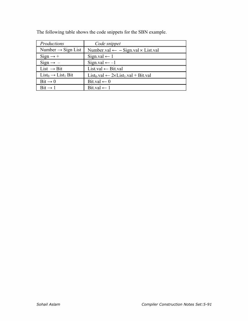
Sohail Aslam Compiler Construction Notes Set:5-91
The following table shows the code snippets for the SBN example.
Productions Code snippet Number → Sign List Number.val ← – Sign.val × List.val Sign → + Sign.val ← 1 Sign → – Sign.val ← –1 List → Bit List.val ← Bit.val List0 → List1 Bit List0.val ← 2×List1.val + Bit.val Bit → 0 Bit.val ← 0 Bit → 1 Bit.val ← 1
Sohail Aslam Compiler Construction Notes Set:5-90
LLeeccttuurree 3333 Implementing Ad-Hoc Scheme
The parser needs a mechanism to pass values of attributes from definitions in one snippet to uses in another. We will adopt notation used by YACC for snippets and passing values. Recall that the skeleton LR(1) parser stored two values on the stack ⟨symbol,state⟩. We can replace this with triples ⟨value,symbol,state⟩. On a reduction by A → β, the parser pops 3×|β| items from the stack rather than 2×|β|. It pushes value along with the symbol.

Sohail Aslam Compiler Construction Notes Set:5-90
LLeeccttuurree 3344 Let’s go through an example of using YACC to implement the ad-hoc scheme for an arithmetic calculator. The YACC file for a calculator grammar is as follows: %token NUMBER LPAREN RPAREN %token PLUS MINUS TIMES DIVIDE %% expr : expr PLUS expr | expr MINUS expr | expr TIMES expr | expr DIVIDE expr | LPAREN expr RPAREN | MINUS expr | NUMBER ; %% We will add the code snippets %{ #include <iostream> %} // type of value entries in the parse stack %union {int val;} %token NUMBER LPAREN RPAREN EQUAL %token PLUS MINUS TIMES DIVIDE /* associativity and precedence:in order of increasing precedence */ %nonassoc EQUAL %left PLUS MINUS %left TIMES DIVIDE %left UMINUS /* dummy token to use as precedence marker */ %type <val> NUMBER expr %% prog : expr { cout << $1 << endl;} ; expr : expr PLUS expr {$$ = $1 + $3;} | expr MINUS expr {$$ = $1 - $3;}

Sohail Aslam Compiler Construction Notes Set:5-91
| expr TIMES expr {$$ = $1 * $3;} | expr DIVIDE expr {if($3) $$ = $1 / $3;} | LPAREN expr RPAREN {$$ = $2;} | MINUS expr {$$ = -$2;} | NUMBER {$$ = $1;} ; The ‘$’ notation is used by YACC to refer to values of symbols on the right hand side of the grammar production. For example, for expr : expr PLUS expr, $1 refers to first expr on the right, $2 refers to PLUS and $3 refers to the second non-terminal expr. The notation $$ refers to the symbol on the left hand side of the production. Internally, the $1 refers to the attribute value associated with the first grammar symbol, $2 with the second, $3 with the third and so on. These values are stored in the parse stack. The notation $$ instructs YACC to push a computed attribute value on the stack and associate it with the symbol on the left when the reduction takes place. The following attributed tree shows the values as they are computed in a bottom-up parse
(note: please see the file “lex_yacc.pdf” for additional information on using YACC.)
3 2 4×+
E
E E
val=3
val=4
E val=8
val=2
E val=11

Sohail Aslam Compiler Construction Notes Set:5-92
Intermediate Representations Compilers are organized as a series of passes. This creates the need for an intermediate representation (IR) for the code being compiled. Compilers use some internal form– an IR –to represent the code being analyzed and translated. Many compilers use more than one IR during the course of compilation. The IR must be expressive enough to record all of the useful facts that might be passed between passes of the compiler. During translation, the compiler derives facts that have no representation in the source code. For example, the addresses of variables and procedures are not specified in the code being compiled. Typically, the compiler augments the IR with a set of tables that record additional information. Foremost among these is the symbol table. These tables are considered part of the IR Selecting an appropriate IR for a compiler project requires an understanding of both the source language and the target machines and the properties of the programs to be compiled. Thus, a source-to-source translator e.g., C++ to Java, might keep its internal information in a form quite to close to the source. In contrast, a compiler that produces assembly code might use a form close to the target machine’s instruction set.

Sohail Aslam Compiler Construction Notes Set:5-90
LLeeccttuurree 3355 IR Taxonomy
IRs fall into three organizational categories:
1. Graphical IRs encode the compiler’s knowledge in a graph. 2. Linear IRs resemble pseudo-code for some abstract machine 3. Hybrid IRs combine elements of both graphical (structural) and linear IRs
Graphical IRs
Parse trees are graphs that represent source-code form of the program. The structure of the tree corresponds to the syntax of the source code. Parse trees are used primarily in discussion of parsing and in attribute grammar systems where they are the primary IR In most other applications, compilers use one of the more concise alternatives. An abstract syntax tree (AST) retains the essential structure of the parse tree but eliminates extraneous nodes. Here, for example, is the AST for the expression a = b*-c + b*-c. Notice how all derivation related information has been removed.
ASTs have been used in many practical compiler systems such as source-to-source systems, automatic parallelization tools, pretty-printing etc. AST is more concise than a parse tree. It faithfully retains the structure of the original source code. Consider the AST for x*2+x*2*y
=
a +
* b -
c
*b -
c
+
*
x 2
*
y*
2x

Sohail Aslam Compiler Construction Notes Set:5-91
The AST contains two distinct copies of x*2.A directed acyclic graph (DAG) is a contraction of the AST that avoids duplication.
If the value of x does not change between uses of x*2, the compiler can generate code that evaluates the subtree once and uses the result twice. The task of building AST fits neatly into an ad hoc-syntax-directed translation scheme. Assume that the compiler has routines mknode and mkleaf for creating tree nodes. The following rules can be attached to the expression grammar to create AST.
Production Semantic Rule E → E1 + E2 E.nptr = mknode(‘+’, E1.nptr, E2.nptr) E → E1 ∗ E2 E.nptr = mknode(‘∗’, E1.nptr, E2.nptr) E → – E1 E.nptr = mknode(‘–’, E1.nptr) E → ( E1 ) E.nptr = E1.nptr E → num E.nptr = mkleaf(‘num’, num.val)
The following table shows the same rules using YACC syntax.
Production Semantic Rule (yacc) E → E1 + E2 $$.nptr = mknode(‘+’, $1.nptr, $3.nptr)
E → E1 ∗ E2 $$.nptr = mknode(‘∗’, $1.nptr, $3.nptr) E → – E1 $$.nptr = mknode(‘–’, $1.nptr) E → ( E1 ) $$.nptr = $1.nptr E → num $$.nptr = mkleaf(‘num’, $1.val)
We will use another IR, called three-address code, for actual code generation The semantic rules for generating three-address code for common programming languages constructs are similar to those for AST. Linear IRs
The alternative to graphical IR is a linear IR. An assembly-language program is a form of linear code. It consists of a sequence of instructions that execute in order of appearance
+
*
y*
2x

Sohail Aslam Compiler Construction Notes Set:5-92
Two linear IRs used in modern compilers are stack-machine code and three-address code. Stack-machine code is sometimes called one-address code. It assumes the presence of an operand stack. Most operations take their operands from the stack and push results back onto the stack. Here, for example, is the linear IR for x – 2 × y
stack-machine three-address push 2 t1 ← 2 push y t2 ← y multiply t3 ← t1 × t2 push x t4 ← x subtract t5 ← t4 – t1
Stack-machine code is compact; it eliminates many names from IR. This shrinks the program in IR form. All results and arguments are transitory unless explicitly moved to memory. Stack-machine code is simple to generate and execute. Smalltalk-80 and Java use byte-codes which are abstract stack-machine code. The byte-code is either interpreted or translated into target machine code (JIT). In three-address code most operations have the form x ← y op z with an operator (op), two operands (y and z) and one result (x). Some operators, such as an immediate load and a jump, will need fewer arguments.

Sohail Aslam Compiler Construction Notes Set:6-104
LLeeccttuurree 3366 Three-address code is attractive for several reasons. Absence of destructive operators gives the compiler freedom to reuse names and values. Three-address code is reasonably compact: operations are 1 to 2 bytes; addresses are 4 bytes. Many modern processors implement three-address operations; a three-address code models their properties well We now consider syntax-directed translation schemes using three-address code for various programming constructs. We start with the assignment statement. Assignment Statement
Production translation scheme S → id = E { p = lookup(id.name); emit( p, ‘=’, E.place); } E → E1 + E2 { E.place = newtemp();
emit( E.place, ‘=’, E1.place,‘+’, E2.place); } E → E1 ∗ E2 { E.place = newtemp();
emit( E.place, ‘=’, E1.place, ‘∗’, E2.place); } E → – E1 { E.place = newtemp();
emit( E.place, ‘=’, ‘–’ ,E1.place); } E → ( E1 ) { E.place = E1.place; } E → id { p = lookup(id.name); emit( E.place, ‘=’, p ); }
The translation scheme uses a symbol table for identifiers and temporaries. Every time the parser encounters an identifier, it installs it in the symbol table. The symbol table can be implemented as a hash table or using some other efficient data structure for table. The routine lookup(name) checks if there an entry for the name in the symbol table. If the name is found, the routine returns a pointer to entry. The routine newtemp() returns a new temporary in response to successive calls. Temporaries can be placed in the symbol table. The routine emit() generates a three-address statement which can either be held in memory or written to a file. The attribute E.place records the symbol table location.
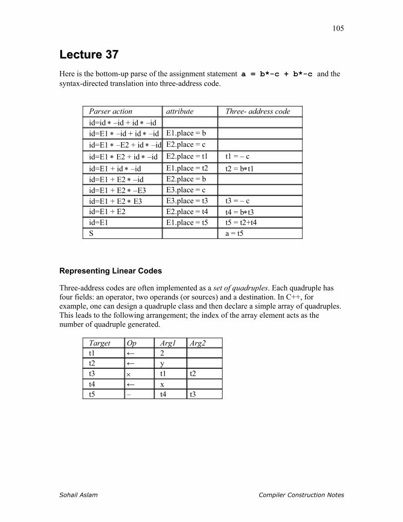
Sohail Aslam Compiler Construction Notes
105
LLeeccttuurree 3377 Here is the bottom-up parse of the assignment statement a = b*-c + b*-c and the syntax-directed translation into three-address code.
Parser action attribute Three- address code id=id ∗ –id + id ∗ –id id=E1 ∗ –id + id ∗ –id E1.place = b id=E1 ∗ –E2 + id ∗ –id E2.place = c id=E1 ∗ E2 + id ∗ –id E2.place = t1 t1 = – c id=E1 + id ∗ –id E1.place = t2 t2 = b∗t1 id=E1 + E2 ∗ –id E2.place = b id=E1 + E2 ∗ –E3 E3.place = c id=E1 + E2 ∗ E3 E3.place = t3 t3 = – c id=E1 + E2 E2.place = t4 t4 = b∗t3 id=E1 E1.place = t5 t5 = t2+t4 S a = t5
Representing Linear Codes
Three-address codes are often implemented as a set of quadruples. Each quadruple has four fields: an operator, two operands (or sources) and a destination. In C++, for example, one can design a quadruple class and then declare a simple array of quadruples. This leads to the following arrangement; the index of the array element acts as the number of quadruple generated.
Target Op Arg1 Arg2 t1 ← 2 t2 ← y t3 × t1 t2 t4 ← x t5 – t4 t3

Sohail Aslam Compiler Construction Notes
106
An array of pointers to quads can be employed which leads to the following structure:
Both simple array and array of pointers have maximum size limitation. This limitation can be overcome by using a linked list of quads:
Flow-of-Control Statements
We now use the syntax-directed translation scheme for the flow-of-control statements found in most procedural programming languages. S → if E then S1
| if E then S1 else S2
| while E do S1
where E is a boolean expression. Consider the statement
if c < d then x = y + z else x = y – z
t1 ← 2 •
t2 ← y •
t3 × t1 t2 •
t4 ← x •
t5 – t4 t3 •
t1 ← 2 •
t2 ← y •
t3 × t1 t2 •
t4 ← x •
t5 – t4 t3 •
•
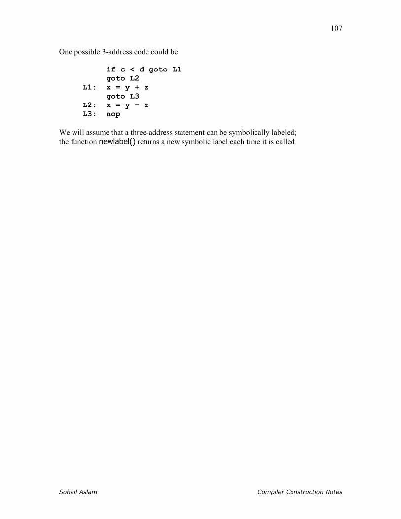
Sohail Aslam Compiler Construction Notes
107
One possible 3-address code could be
if c < d goto L1 goto L2 L1: x = y + z goto L3 L2: x = y – z L3: nop
We will assume that a three-address statement can be symbolically labeled; the function newlabel() returns a new symbolic label each time it is called

Sohail Aslam Compiler Construction Notes Set:6-108
108
LLeeccttuurree 3388 Three-Address Statement Types
Prior to proceeding with flow-of-control construct, here are the types of three-Address statements that we will use
• Assignment statement x = y op z
op is a binary arithmetic or logical operation
• Copy statement x = y
value of y is assigned to x
• Unconditional jump goto L
The three-address statement with label L is executed next
• Conditional jump if x relop y goto L
relop is <, =, >=, etc. If x stands in relation relop to y, execute statement with label L, next otherwise
• Indexed assignment
a) x = y[i] b) x[i] = y In a), set x to value in location i memory units beyond location y. In b), set contents of location i memory units beyond x to y. We associate with a boolean expression E two labels (attributes); E.true and E.false. The control flows to E.true if the expression evaluates to true, to E.false otherwise. Following is syntax-directed translation for
S → if E then S1
E.true = newlabel()
E.false = S.next S1.next = S.next S.code = E.code || gen(E.true ‘:’) || S1.code The attribute “next” records the label of the next statement to execute. “code” is string-valued attribute that holds the actual code generated in the form of a character string. The code can be eventually written out to a file. The || is the string concatenation operator, that is “hello”|| “ world” will yield the combined string “hello world”.
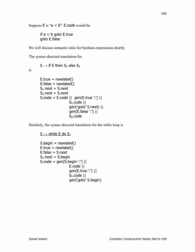
Sohail Aslam Compiler Construction Notes Set:6-109
109
Suppose E is “a < b”. E.code would be if a < b goto E.true goto E.false We will discuss semantic rules for boolean expressions shortly The syntax-directed translation for
S → if E then S1 else S2 is
E.true = newlabel() E.false = newlabel() S1.next = S.next S2.next = S.next S.code = E.code || gen(E.true ‘:’) || S1.code || gen(‘goto’ S.next) || gen(E.false ‘:’) || S2.code
Similarly, the syntax-directed translation for the while loop is
S → while E do S1
S.begin = newlabel() E.true = newlabel() E.false = S.next S1.next = S.begin S.code = gen(S.begin ‘:’) || E.code || gen(E.true ‘:’) || S1.code || gen(‘goto’ S.begin)

Sohail Aslam Compiler Construction Notes Set:6-110
110
LLeeccttuurree 3399 Boolean Expressions
In programming languages, boolean expressions have two primary purposes: • compute logical values such as x = a < b && d > e • conditional expressions in flow-of-control statements
Consider the grammar for Boolean expressions E → E or E | E and E | not E | ( E ) | id relop id | true | false We will implement the translation for boolean expressions by flow of control method, i.e., representing the value of a boolean expression by a position reached in the program. Here are the syntax directed translation for the grammar rules E → id1 relop id2
E.code = gen(‘if’ id1 relop id2 ‘goto’ E.true) || gen(‘goto’ E.false) E → true E.code = gen(‘goto’ E.true) E → false E.code = gen(‘goto’ E.false) E → E1 or E2
E1.true = E.true E1.false = newlabel() E2.true = E.true E2.false = E.false E.code = E1.code || gen(E1.false ‘:’) || E2.code
E → E1 and E2
E1.true = newlabel() E1.false = E.false E2.true = E.true E2.false = E.false E.code = E1.code ||gen(E1.true ‘:’) || E2.code

Sohail Aslam Compiler Construction Notes Set:6-111
111
E → not E1
E1.true = E.false E1.false = E.true E.code = E1.code
E → ( E1 )
E1.true = E.true E1.false = E.false E.code = E1.code
Example: Consider the expression a < b or c < d and e < f Suppose the true and false exits for the entire expression are Ltrue and Lfalse. The syntax directed translation scheme will generate the code
if a < b goto Ltrue goto L1 L1: if c < d goto L2 goto Lfalse L2: if e < f goto Ltrue goto Lfalse
Example: Consider the while statement
while a < b if c < d then x = y + z else x = y – z
The translation scheme will generate the following code:
L1: if a < b goto L2 goto Lnext L2: if c < d goto L3 goto L4 L3: t1 = y + z x = t1 goto L1 L4: t2 = y – z x = t2 goto L1 Lnext: nop
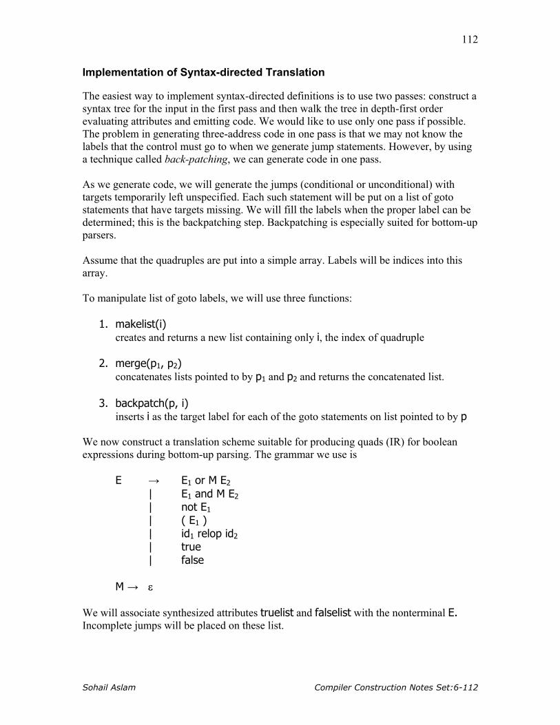
Sohail Aslam Compiler Construction Notes Set:6-112
112
Implementation of Syntax-directed Translation
The easiest way to implement syntax-directed definitions is to use two passes: construct a syntax tree for the input in the first pass and then walk the tree in depth-first order evaluating attributes and emitting code. We would like to use only one pass if possible. The problem in generating three-address code in one pass is that we may not know the labels that the control must go to when we generate jump statements. However, by using a technique called back-patching, we can generate code in one pass. As we generate code, we will generate the jumps (conditional or unconditional) with targets temporarily left unspecified. Each such statement will be put on a list of goto statements that have targets missing. We will fill the labels when the proper label can be determined; this is the backpatching step. Backpatching is especially suited for bottom-up parsers. Assume that the quadruples are put into a simple array. Labels will be indices into this array. To manipulate list of goto labels, we will use three functions:
1. makelist(i) creates and returns a new list containing only i, the index of quadruple
2. merge(p1, p2) concatenates lists pointed to by p1 and p2 and returns the concatenated list.
3. backpatch(p, i) inserts i as the target label for each of the goto statements on list pointed to by p
We now construct a translation scheme suitable for producing quads (IR) for boolean expressions during bottom-up parsing. The grammar we use is
E → E1 or M E2 | E1 and M E2 | not E1 | ( E1 ) | id1 relop id2 | true | false
M → ε We will associate synthesized attributes truelist and falselist with the nonterminal E. Incomplete jumps will be placed on these list.

Sohail Aslam Compiler Construction Notes Set:6-113
113
We associate the semantic action { M.quad = nextquad() } with the production M → ε. The function nextquad() returns the index of the next quadruple to follow. The attribute quad will record this index.
1. E → E1 and M E2
{ backpatch(E1.truelist, M.quad); E.truelist = E2.truelist; E.falselist = merge(E1.falselist, E2.falselist); } Let’s look at the mechanics. If E1 is false, E is false because of the and clause. If E1 is true, we need to evaluate E2. The start of E1, i.e., the index of the first quad for E1 is recorded by M.quad; in a bottom up parse, the reduction M → ε will occur before reduction to E2. The backpatch sets the targets of goto’s in E1.truelist to the start of E2.
2. E → E1 or M E2
{ backpatch(E1.falselist, M.quad); E.truelist = merge(E1.truelist, E2.truelist); E.falselist = E2.falselist; }
3. E → not E1 { E.truelist = E1.falselist; E.falselist = E1.truelist; }
4. E → ( E1 ) { E.truelist = E1.truelist; E.falselist = E1.falselist; }
5. E → id1 relop id2 { E.truelist = makelist(nextquad()); E.falselist = makelist(nextquad()+1); emit(‘if’ id1 relop id2 ‘goto _’) ; emit(‘goto _’ ); }

Sohail Aslam Compiler Construction Notes Set:6-114
114
6. E → true { E.truelist = makelist(nextquad()); emit(‘goto _’ ); }
7. E → false { E.falselist = makelist(nextquad()); emit(‘goto _’ ); }

Sohail Aslam Compiler Construction Notes Set:6-115
115
LLeeccttuurree 4400 Example: consider, the boolean expression a < b or c < d and e < f Recall the syntax directed translation for the production
E → id1 relop id2
{ E.truelist = makelist(nextquad()); E.falselist = makelist(nextquad()+1); emit(‘if’ id1 relop id2 ‘goto _’) ; emit(‘goto _’ ); }
We carry out a bottom-up parse. In response to reduction of a < b to E, the list E.truelist gets {100} and E.falselist gets {101} and the two quadruples 100: if a < b goto _ 101: goto _ are generated. Notice that the goto’s are generated with targets. These are precisely the goto’s whose quad indices 100 and 101 are recorded in the truelist and falselist attributes of E. These will be patched later in the parse via the backpatching mechanism. The next reduction to happen is M → ε which is in the production E → E1 or M E2
This reduction will eventually take place when reduction to E2 happens. This marker non-terminal M records the value of nextquad which at this time is 102. Next, the reduction of c < d to E leads to the list E.truelist getting {102}, E.falselist getting {103} and the two quadruples 102: if c < d goto _ 103: goto _ are generated. Next reduction is M → ε. Τhe marker non-terminal M in the production E → E1 and M E2

Sohail Aslam Compiler Construction Notes Set:6-116
116
records the value of nextquad which at this time is 104, the quad index of first quad of E2 . Reducing e < f to E causes E.truelist to get {104}, E.falselist to get {105} and the generation of quads 104: if e < f goto _ 105: goto _ We now reduce by the production E → E1 and M E2 Recall the semantic actions associated with this rule:
E → E1 and M E2
{ backpatch(E1.truelist, M.quad); E.truelist = E2.truelist; E.falselist = merge(E1.falselist, E2.falselist); }
The six quadruples generated so far are 100: if a < b goto _ 101: goto _ 102: if c < d goto _ 103: goto _ 104: if e < f goto _ 105: goto _ The semantic action calls backpatch({102},104) The backpatch fills in 104 as the target of the goto in quad 102. 100: if a < b goto _ 101: goto _ 102: if c < d goto 104 103: goto _ 104: if e < f goto _ 105: goto _ The next two semantic actions define E.truelist and E.falselist. This way, the synthesized attributes propagate the attributes up the parse tree. We now reduce by the production

Sohail Aslam Compiler Construction Notes Set:6-117
117
E → E1 or M E2 The semantic action calls backpatch({101},102) which fills in 102 in statement 101: 100: if a < b goto _ 101: goto 102 102: if c < d goto 104 103: goto _ 104: if e < f goto _ 105: goto _ The remaining goto’s will have their targets backpatched later in the parse. The attributed parse tree at this stage is
E.t = {100, 104}E.f = {103, 105}
E.t = {100} E.f = {101}
E.t = {104} E.f = {103, 105}
E.t = {102}E.f = {103}
E.t = {104}E.f = {105}
c < d
a < b
e < f
M.q = 104
M.q = 102or
and
ε
ε

Sohail Aslam Compiler Construction Notes Set:6-118
118
LLeeccttuurree 4411 Flow-of-Control Statements
We now use backpatching to translate flow-of-control statements in one pass. We will use the same list-handling procedures as before. S → if E then S | if E then S else S | while E do S | begin L end | A L → L ; S | S The semantic actions associated with each production are
1. S → if E then M1 S1 N else M2 S2
{ backpatch(E.truelist, M1.quad); backpatch(E.falselist, M2.quad); S.nextlist = merge(S1.nextlist, merge( N.nextlist,S2.nextlist)); }
2. N → ε { N.nextlist = makelist(nextQuad()); emit(‘goto_’); }
3. M → ε { M.quad = nextQuad(); }
4. S → if E then M S1 { backpatch(E.truelist, M.quad); S.nextlist = merge(E.falselist,S1.nextlist); }
5. S → while M1 E do M2 S1 {

Sohail Aslam Compiler Construction Notes Set:6-119
119
backpatch(S1.nextlist, M1.quad); backpatch(E.truelist, M2.quad); S.nextlist = E.falselist; emit( ‘goto’ M1.quad); }
6. S → begin L end { S.nextlist = L.nextlist; }
7. S → A { S.nextlist = nil; }
8. S → L1 ; M S { backpatch(L1.nextlist, M.quad); L.nextlist = S.nextlist; }
9. L → S { L.nextlist = S.nextlist; }
Example: Let go through the example with the following input statement
if a < b or c < d and e < f then x = y+z else x = y-z The bottom-up parse will reduce the compound boolean expression a < b or c < d and e < f to E1 or M E2 which we have already covered in the previous example. We thus assume that the quads for the boolean expression have been generated. The sentential form at this stage is
if E1 or M E2 then x = y+z else x = y-z The reduction E → E1 or M E2 yields
if E then x = y+z else x = y-z The semantic actions define the synthesized attributes E.truelist=[100,104] and E.falselist=[103,105].

Sohail Aslam Compiler Construction Notes Set:6-120
120
We now trace the remaining bottom up parse and execute the semantic actions:
if E then M1 x=y+z else x=y-z M1 → ε { M1.quad = 106 } ⇒ if E then M1 A else x=y-z A → x=y+z { emit(‘x=y+z’) } ⇒ if E then M1 S1 else A S1 → A { S1.nextlist = nil} ⇒ if E then M1 S1 N else x=y-z N → ε { N.nextlist = [107] emit(‘goto _’ } ⇒ if E then M1 S1 N else M2 x=y-z M2 → ε { M2.quad = 108 } ⇒ if E then M1 S1 N else M2 A A → x=y-z { emit(‘x=y-z’) } ⇒ if E then M1 S1 N else M2 S2 S2 → A { S2.nextlist = nil } ⇒ S { backpatch([100,104],106) backpatch([103,105],108) S.nextlist=[107]}
The array of quadruples at this stage will contain
100 if a < b goto 106 101 goto 102 102 if c < d goto 104 103 goto 108 104 if e < f goto 106 105 goto 108 106 x=y+z 107 goto _ 108 x=y-z 109

Sohail Aslam Compiler Construction Notes Set:6-121
121
Semantic Actions in YACC
The syntax-directed translation statements can be conveniently specified in YACC The %union will require more fields because the attributes vary. The actual mechanics will be covered in the handout for the syntax-directed translation phase of the course project
122
LLeeccttuurree 4422 Code Generation
The code generation problem is the task of mapping intermediate code to machine code. The generated code must be correct for obvious reasons. It should be efficient both in terms of memory space and execution time. The input to the code generation module of compiler is intermediate code (optimized or not) and its task is typically to produce either machine code or assembly language code for a target machine. The code generation module has to tackle a number of issues.
• Memory management: mapping names to data objects in the run-time system.
• Instruction selection: the assembly language instructions to choose to encode intermediate code statements
• Instruction scheduling: instruction chosen must utilize the CPU resources effectively. Hardware stalls must be avoided.
• Register allocation: operands are placed in registers before executing machine operation such as ADD, MULTIPLY etc. Most processors have a limited set of registers available. The code generator has to make efficient use of this limited resource
For our discussion, we will target a machine that has the following general characteristics. Most actual processors are similar to such architecture. The machine is byte-addressable with 4-byte words. It has N general -purpose registers. It uses two-address instructions of the form op source, destination. The target assembly language operations are:
• MOV source, destination • ADD source, destination • SUB source, destination (dest = dest – source) • GOTO address • CJ conditional jump
More instruction will be added to the instruction set as needed.
Sohail Aslam Compiler Construction Notes Set:7-122

123
The following table presents the addressing modes for source or destination operands.
MODE FORM ADDRESS ADDED COSTabsolute M M 1 register R R 0 indexed c(R) c + contents(R) 1 indirect register *R contents(R) 0 indirect indexed *c(R) contents(c+contents(R)) 1 literal #c c 1 stack SP SP 0 indexed stack c(SP) c + contents(SP) 1
We associate a cost with each instruction. This will allow us to compute the cost of generated code. The cost corresponds to length of instruction. For example the instruction
MOV R0,R1 ; R0 = c(R1) has cost 1 while
MOV R5,M ; M = c(R5) has cost 2: 1 for instruction, 1 additional for memory address. The column title “ADDED COST” indicates this additional cost.
Simple Code Generation
We start with a simple code generation strategy: define a target code sequence for each intermediate code (such as 3-address code) statement type. Thus,
Intermediate code becomes…
a = b MOV b,a a = b[c] MOV addr(b),R0
ADD c, R0 MOV *R0,a
a = b + c MOV b,a ADD c,a
a[b] = c MOV addr(a),R0 ADD b,R0 MOV c,*R0
Sohail Aslam Compiler Construction Notes Set:7-123
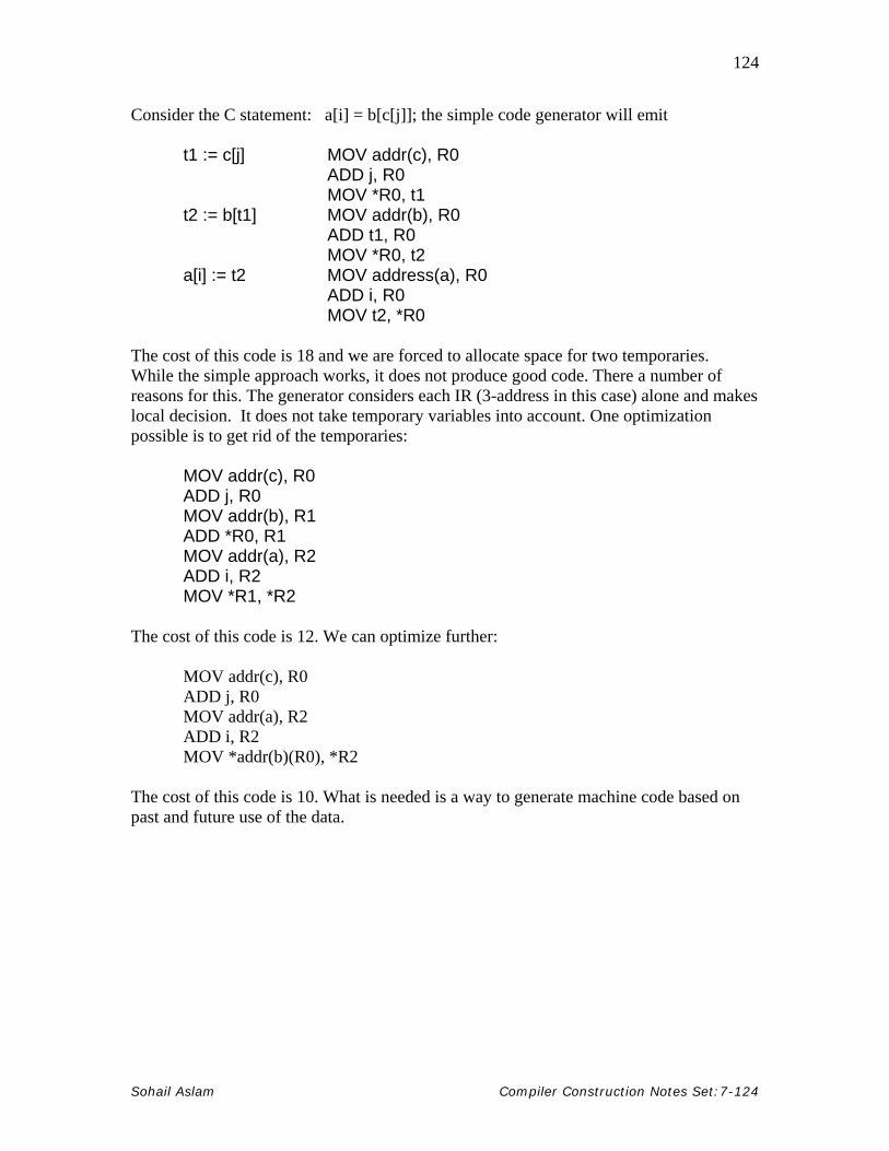
124
Consider the C statement: a[i] = b[c[j]]; the simple code generator will emit t1 := c[j] MOV addr(c), R0 ADD j, R0 MOV *R0, t1 t2 := b[t1] MOV addr(b), R0 ADD t1, R0 MOV *R0, t2 a[i] := t2 MOV address(a), R0 ADD i, R0 MOV t2, *R0 The cost of this code is 18 and we are forced to allocate space for two temporaries. While the simple approach works, it does not produce good code. There a number of reasons for this. The generator considers each IR (3-address in this case) alone and makes local decision. It does not take temporary variables into account. One optimization possible is to get rid of the temporaries:
MOV addr(c), R0 ADD j, R0 MOV addr(b), R1 ADD *R0, R1 MOV addr(a), R2 ADD i, R2 MOV *R1, *R2
The cost of this code is 12. We can optimize further:
MOV addr(c), R0 ADD j, R0 MOV addr(a), R2 ADD i, R2 MOV *addr(b)(R0), *R2
The cost of this code is 10. What is needed is a way to generate machine code based on past and future use of the data.
Sohail Aslam Compiler Construction Notes Set:7-124

125
LLeeccttuurree 4433 Control Flow Graph - CFG
A control flow graph is the triplet CFG = < V, E, Entry >, where V = vertices or nodes, representing an instruction or basic block (group of statements), E = (V x V) edges, potential flow of control. Entry is an element of V, the unique program entry. Basic Blocks
A basic block is a sequence of consecutive statements with single entry/single exit. Flow of control only enters at the beginning and only leaves at the end. The can be variants of basic blocks with single entry/multiple exit, multiple entry/single exit. Generating CFGs
In order to generate a CFG, we partition the intermediate code (3-address code, for example) into basic blocks. Edges are added corresponding to control flow between blocks. An unconditional goto in the IR will lead to a single edge to another or the same block. A conditional goto will lead to multiple edges. If there is no goto at the end of a block, the control passes to first statement of next block. Here is the algorithm for partitioning intermediate code into basic blocks. The input to the algorithm is a sequence of three-address statements. The algorithm will output a list of basic blocks with each three-address statements in exactly one block. Algorithm: partition 3-address statements into basic blocks:
1. Determine the set of leaders – the first statements of basic blocks. The rules are:
• The first statement is a leader • Any statement that is the target of a conditional or unconditional goto is a
leader • Any statement that immediately follows a goto or conditional goto is a
leader
2. For each leader, its basic block consists of the leader and all statements up to but not including the next leader or the end of the program
Sohail Aslam Compiler Construction Notes Set:7-125
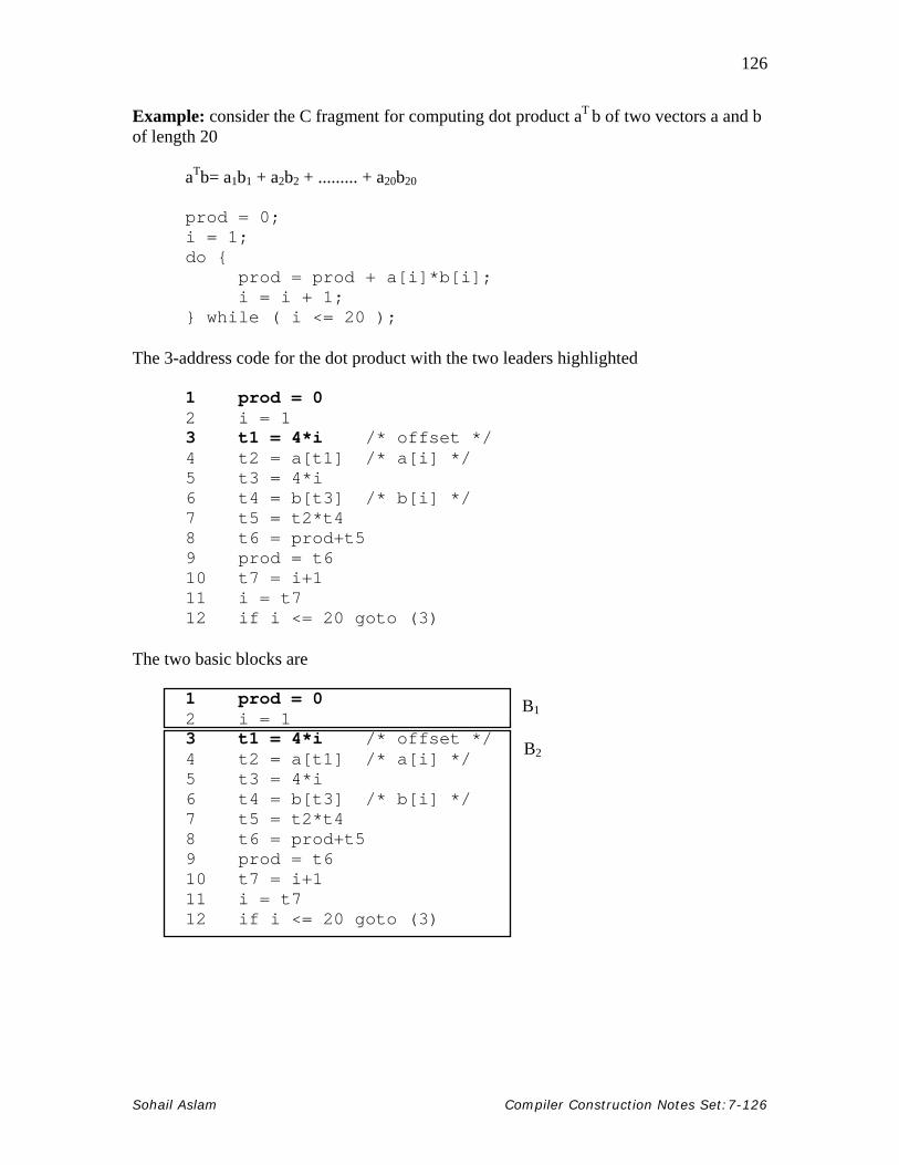
126
Example: consider the C fragment for computing dot product aT b of two vectors a and b of length 20 aTb= a1b1 + a2b2 + ......... + a20b20
prod = 0; i = 1; do { prod = prod + a[i]*b[i]; i = i + 1; } while ( i <= 20 );
The 3-address code for the dot product with the two leaders highlighted
1 prod = 0 2 i = 1 3 t1 = 4*i /* offset */ 4 t2 = a[t1] /* a[i] */ 5 t3 = 4*i 6 t4 = b[t3] /* b[i] */ 7 t5 = t2*t4 8 t6 = prod+t5 9 prod = t6 10 t7 = i+1 11 i = t7 12 if i <= 20 goto (3)
The two basic blocks are
1 prod = 0 2 i = 1 3 t1 = 4*i /* offset */ 4 t2 = a[t1] /* a[i] */ 5 t3 = 4*i 6 t4 = b[t3] /* b[i] */ 7 t5 = t2*t4 8 t6 = prod+t5 9 prod = t6 10 t7 = i+1 11 i = t7 12 if i <= 20 goto (3)
BB1
BB2
Sohail Aslam Compiler Construction Notes Set:7-126

127
This yields the following CFG; note that the target of the condition goto at the end of the second block has been replaced by reference to block 2.
prod = 0 i = 1
t1 = 4*i t2 = a[t1] t3 = 4*i t4 = b[t3] t5 = t2*t4 t6 = prod+t5 prod = t6 t7 = i+1 i = t7 if i <= 20 goto B2
B1
B2
Let us consider a more complex example. Here is the quicksort algorithm encoded as a recursive function in C++
i = 1 Quick Sort void quicksort(int m, int n) { int i,j,v,x; if( n <= m ) return; i=m-1; j=n; v=a[n]; while(true) { do i=i+1; while( a[i] < v); do j=j-1; while( a[j] > v); i( i >= j ) break; x=a[i]; a[i]=a[j]; a[j]=x; } x=a[i]; a[i]=a[n]; a[n]=x; quicksort(m,j); quicksort(i+1,n); }
Sohail Aslam Compiler Construction Notes Set:7-127

128
The 3-address for the highlighted portion of the routine (the recursive calls have been left out) with the leaders highlighted and the resulting CFG is
(1) i := m – 1 (16) t7 := 4 * i (2) j := n (17) t8 := 4 * j (3) t1 := 4 * n (18) t9 := a[t8] (4) v := a[t1] (19) a[t7] := t9 (5) i := i + 1 (20) t10 := 4 * j (6) t2 := 4 * i (21) a[t10] := x (7) t3 := a[t2] (22) goto (5) (8) if t3 < v goto (5) (23) t11 := 4 * i (9) j := j - 1 (24) x := a[t11] (10) t4 := 4 * j (25) t12 := 4 * i (11) t5 := a[t4] (26) t13 := 4 * n (12) If t5 > v goto (9) (13) if i >= j goto (23) (28) a[t12] := t14
(27) t14 := a[t13]
(14) t6 := 4*i (29) t15 := 4 * n (16) x := a[t6] (30) a[t15] := x
Basic Block Code Generation
The code generation can carried out at the basic block level. A number of strategies are available to generate code from a basic block. The three we will discuss are
1. Basic - using liveness information 2. Using DAGS - node numbering 3. Register Allocation
In case of the basic code generation strategy, the generator deals with each basic block individually to emit machine code for the block using liveness information. At the end of the block, the generator emits code to save any live values left in registers. Computing Live/Next Use Information
For the statement: x = y + z x has a next use if there is a statement s that references x and there is some way for control to flow from the original statement to s.
x = y + z ...... ...... s t1 = x – t3
Sohail Aslam Compiler Construction Notes Set:7-128

129
A variable is live at a given point in time if it has a next use. Liveness tells us whether we care about the value held by a variable. Here is the algorithm for computing live status of variables in a basic block” Algorithm: Computing live status Input: A basic block. Output: For each statement, set of live variables Method: 1. Initially all non-temporary variables go into live set. 2. for i = last statement to first statement: for statement i: x = y op z
attach to statement i, current live set. remove x from set. add y and z to set.
Sohail Aslam Compiler Construction Notes Set:7-129

130
LLeeccttuurree 4444 Example: let us apply the algorithm to the following segment of 3-address code: a = b + c t1 = a * a b = t1 + a c = t1 * b t2 = c + b a = t2 + t2
live = {b,c} a = b + c live = {a} t1 = a * a live = {a,t1} b = t1 + a live = { b,t1} c = t1 * b live = {b,c} t2 = c + b live = {b,c,t2} a = t2 + t2 live = {a,b,c}
Basic Code Generation
With live/next use information computed, the basic code generation algorithm proceeds as follows. Process the 3-address instructions from beginning to end of a block. For each instruction, use machine registers to hold operands whenever possible. A non-live value in a register can be discarded, freeing that register. The code generator uses two data structures for keeping track of register usage:
1. Register descriptor - register status (empty, inuse) and contents (one or more "values")
2. Address descriptor - the location (or locations) where the current value for a variable can be found (register, stack, memory)
Instruction type: x = y op z 1. If y is non-live and in register R (alone) then generate OP z’, R
Sohail Aslam Compiler Construction Notes Set:7-130

131
where z’ = best location for z. i.e., lookup address descriptor for z. Prefer register location if z is present in a register. 2. If operation is commutative, z is non-live and is in register R (alone), generate OP y’, R (y’ = best location for y) 3. If there is a free register R, generate MOV y’, R OP z’, R 4. Use a memory location. Generate MOV y’,x OP z’,x After generating machine instructions, update information about the current best location of x. If x is in a register, update that register’s information (descriptor). If y and/or z are not live after this instruction, update register and address descriptors according. Let us return to the 3-address code example and apply the basic code generation algorithm. Recall the basic block with liveness information:
live = {b,c} a = b + c live = {a} t1 = a * a live = {a,t1} b = t1 + a live = { b,t1} c = t1 * b live = {b,c} t2 = c + b live = {b,c,t2} a = t2 + t2 live = {a,b,c}
Initially
three registers: ( -, -, -) all empty current values: (a,b,c,t1,t2) = (m,m,m, -, -)
Sohail Aslam Compiler Construction Notes Set:7-131

132
1: a = b + c, Live = a getreg(): L = R1 MOV b,R1 ADD c,R1 ; R1 := R1 + c Registers: (a, -, -) current values: (R1,m,m, -, -)
2: t1 = a * a,
Live = a,t1 L = R2 (since a is live) MOV R1,R2 MUL R2,R2 ; R2 = R2* R2 Registers: (a,t1, -) current values: (R1,m,m,R2, -)
3: b = t1 + a,
Live = b,t1 Since a is not live L = R1 ADD R2,R1 ; R1 = R1+R2 Registers: (b,t1, -) current values: (m,R1,m,R2, -)
4: c = t1 * b,
Live = b,c Since t1 is not live L = R2 MUL R1,R2 ; R2 = R1*R2 Registers: (b,c, -) current values: (m,R1,R2, -, -)
5: t2 = c + b,
Live = b,c,t2 L = R3 MOV R2,R3 ADD R1,R3 ; R3 = R1+R2 Registers: (b,c,t2) current values: (m,R1,R2, -,R3)
6: a = t2 + t2,
Live = a,b,c ADD R3,R3 Registers: (b,c,a) current values: (R3,R1,R2,-,R3)
Sohail Aslam Compiler Construction Notes Set:7-132
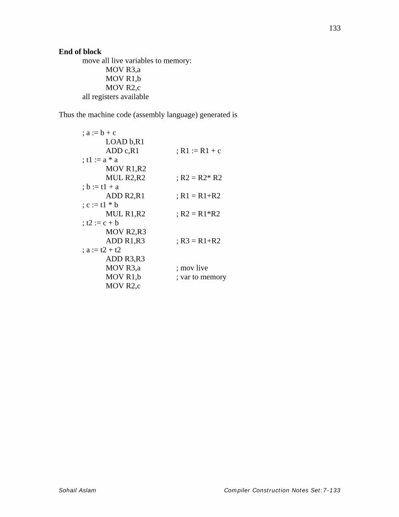
133
End of block move all live variables to memory: MOV R3,a MOV R1,b MOV R2,c all registers available
Thus the machine code (assembly language) generated is
; a := b + c
LOAD b,R1 ADD c,R1 ; R1 := R1 + c
; t1 := a * a MOV R1,R2 MUL R2,R2 ; R2 = R2* R2 ; b := t1 + a ADD R2,R1 ; R1 = R1+R2 ; c := t1 * b MUL R1,R2 ; R2 = R1*R2 ; t2 := c + b MOV R2,R3 ADD R1,R3 ; R3 = R1+R2 ; a := t2 + t2 ADD R3,R3 MOV R3,a ; mov live
MOV R1,b ; var to memory MOV R2,c
Sohail Aslam Compiler Construction Notes Set:7-133

134
LLeeccttuurree 4455 Liveness information allows us to keep values in registers if they will be used later. An obvious concern is why do we assume all variables are live at the end of blocks? Why do we need to save live variables at the end? It seems reasonable to perceive that we might have to reload them in the next block. To do this, we need to determine live/next use information across blocks and not just within a block. This requires global data-flow analysis. Global Data-Flow Analysis
A Directed Acyclic Graph (DAG) for a basic block has the following labels for the nodes:
• Leaves are labeled by unique identifiers. • Interior nodes are labeled by operator symbols. • Nodes can have multiple labels since they represent computed values.
Algorithm: Generate DAG from 3-address code For statement i: x = y op z
• if y op z node exists, add x to the label for that node. else add node for y op z.
• if y or z exist in the dag, point to existing locations else add leaves for y and/or z and have the op node point to them.
• label the op node with x.
• if x existed previously as a leaf,
subscript that previous entry. • if x is associated with other interior nodes,
remove them from that list.
Sohail Aslam Compiler Construction Notes Set:7-134

135
Here and an example of the DAG generated for the 3-address code
a = b + c t1 = a * a b = t1 + a c = t1 * b t2 = c + b a = t2 + t2
b’
t1
c’
t2
+
*
+ b
*
+
+
c
a
Here is another example
t1 = 4 * i t2 = a[t1] t3 = 4 * i t4 = b[t3] t5 = t2 * t4 t6 = p + t5 p = t6 t7 = i + 1 i = t7 if i <20 goto (1)
a b 4 i’ 1
+ *
< [ ] [ ]
*
+
p’ t5
t2 t4
t1,t3 t7,i
(1)
t6,p
20
Sohail Aslam Compiler Construction Notes Set:7-135

136
DAGs and optimization
DAGs play an important role in code optimization. It is possible to detect common sub-expressions and eliminate them; a node in the DAG with more than one parent is common sub-expression. The order in which the DAG is traversed can lead to better code. For example, the following DAG can be traversed in two ways: The code generated for order one with 2 registers is
MOV a, R0 ADD b,R0 MOV c, R1 ADD D, R1 MOV R0,t1 MOV e, R0 SUB R1,R0 MOV t1,R1 SUB R0, R1 MOV R1,t4
Ten machine instructions are generated.
+a b e
c d
t2 t3
t4
t1
-
- +
Order 1 Order 2 t1 = a + b t2 = c + d t2 = c + d t3 = e – t2 t3 = e – t2 t1 = a + b t4 = t1 – t3 t4 = t1 – t3
Sohail Aslam Compiler Construction Notes Set:7-136

137
Whereas, order #2 with 2 registers leads to
MOV c, R0 ADD D, R0 MOV e, R1 SUB R0,R1 MOV a,R0 ADD b, R0 MOV R0,t4
Only seven instructions are required, a saving of three machine instructions. Reordering improved code because computation of t4 immediately followed computation of t1, its left operand. t1 must be in a register and it is.
Register Allocation
Registers in a machine are a scarce resource. The issue faced by the code generator is this how to best use the bounded number of registers. The matter is complicated by the fact that a few registers are reserved for special purposes. For example, the program counter is kept in a registers. A register is used for the keeping track of the top of the function call stack. Certain operators require multiple registers, often in pairs. Division is an example of such an operator. The general register allocation problem is NP-complete. Heuristic algorithms exist to solve the problem. One such strategy is the by using the graph coloring algorithm: given a graph, color the nodes with different colors such that no two nodes that have an edge between them have the same color. Here is how the graph coloring algorithm can be used to compute register allocation for K registers in a machine. Algorithm: K registers allocation with graph coloring
1. Compute liveness information.
2. Create interference graph G
3. one node for each variable, an edge connects two variables if one is live at a point where the other is defined
4. Simplify: for any node m with less than K neighbors, remove it from the graph and push it onto a stack. If (G - m ) can be colored with K colors, so can G. If we reduce the entire graph, goto step 5.
5. Spill: if we get to the point where we are left with only nodes with degree >= K, mark some node for potential spilling (to memory). Remove and push onto stack. Back to step 3.
Sohail Aslam Compiler Construction Notes Set:7-137
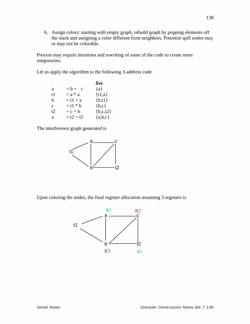
138
6. Assign colors: starting with empty graph, rebuild graph by popping elements off the stack and assigning a color different from neighbors. Potential spill nodes may or may not be colorable.
Process may require iterations and rewriting of some of the code to create more temporaries. Let us apply the algorithm to the following 3-address code live
a = b + c {a} t1 = a * a {t1,a} b = t1 + a {b,t1} c = t1 * b {b,c} t2 = c + b {b,c,t2} a = t2 + t2 {a,b,c}
The interference graph generated is
a
b
t1
c
t2
Upon coloring the nodes, the final register allocation assuming 3 registers is
c
a
b
t1
t2 R1 R3
R1 R2
Sohail Aslam Compiler Construction Notes Set:7-138