Lecture #1

16.31 Feedback Control

Copyright 2001 by Jonathan How.

1

Fall 2001 16.31 1—1

Introduction

K(s) G(s) -6

?

— u(t)

y(t)e(t)r(t)

d(t)

• Goal: Design a controllerK(s) so that the system has some desired

characteristics. Typical objectives:

— Stabilize the system (Stabilization)

— Regulate the system about some design point (Regulation)

— Follow a given class of command signals (Tracking)

— Reduce the response to disturbances. (Disturbance Rejection)

• Typically think of closed-loop control → so we would analyze the

closed-loop dynamics.

— Open-loop control also possible (called “feedforward”) — more

prone to modeling errors since inputs not changed as a result of

measured error.

• Note that a typical control system includes the sensors, actuators,

and the control law.

— The sensors and actuators need not always be physical devices

(e.g., economic systems).

— A good selection of the sensor and actuator can greatly simplify

the control design process.

— Course concentrates on the design of the control law given the

rest of the system (although we will need to model the system).

Fall 2001 16.31 1—2

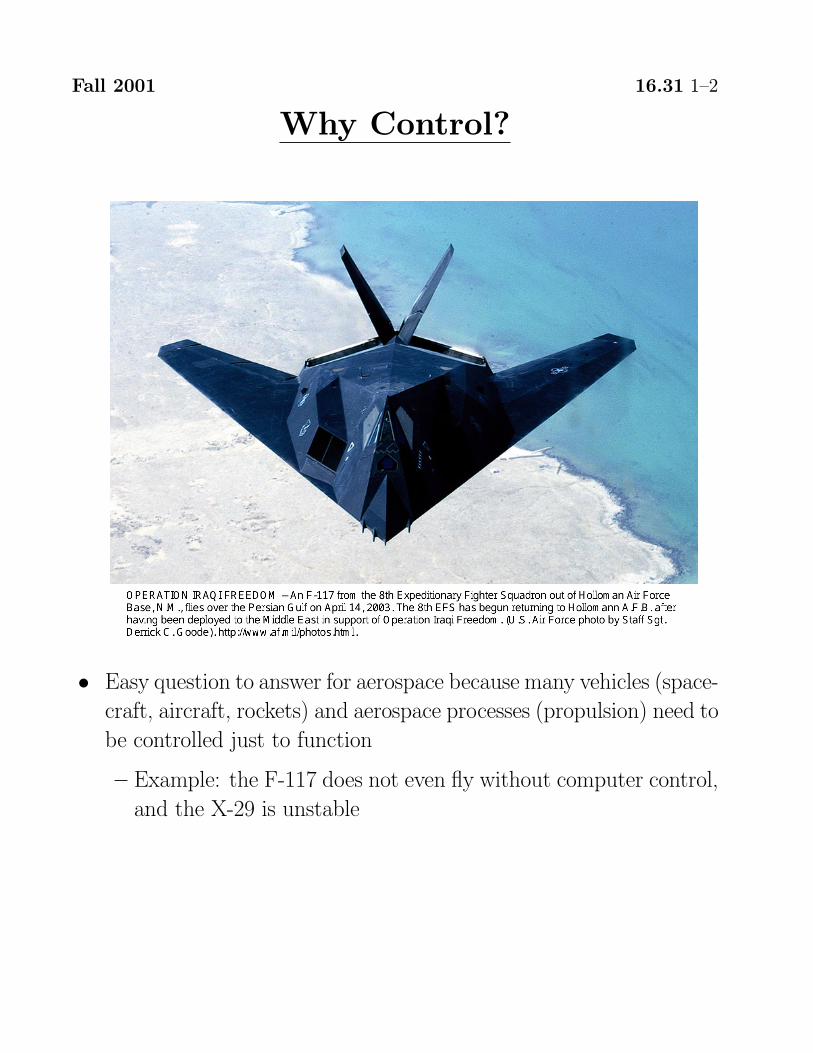
Why Control?

• Easy question to answer for aerospace because many vehicles (space-

craft, aircraft, rockets) and aerospace processes (propulsion) need to

be controlled just to function

— Example: the F-117 does not even fly without computer control,

and the X-29 is unstable

Fall 2001 16.31 1—3

Feedback Control Approach

• Establish control objectives

— Qualitative — don’t use too much fuel

— Quantitative — settling time of step response <3 sec

— Typically requires that you understand the process (expected

commands and disturbances) and the overall goals (bandwidths).

— Often requires that you have a strong understanding of the phys-

ical dynamics of the system so that you do not “fight” them in

appropriate (i.e., inefficient) ways.

• Select sensors & actuators

—What aspects of the system are to be sensed and controlled?

— Consider sensor noise and linearity as key discriminators.

— Cost, reliability, size, . . .

• Obtain model

— Analytic (FEM) or from measured data (system ID)

— Evaluation model → reduce size/complexity→ Design model

— Accuracy? Error model?

• Design controller

— Select technique (SISO, MIMO), (classical, state-space)

— Choose parameters (ROT, optimization)

• Analyze closed-loop performance. Meet objectives?

— Analysis, simulation, experimentation, . . .

— Yes ⇒ done, No⇒ iterate . . .

Fall 2001 16.31 1—4

Example: Blimp Control

• Control objective

— Stabilization

— Red blimp tracks the motion of the green blimp

• Sensors

— GPS for positioning

— Compass for heading

— Gyros/GPS for roll attitude

• Actuators — electric motors (propellers) are very nonlinear.

• Dynamics

— “rigid body” with strong apparent mass effect.

— Roll modes.

• Modeling

— Analytic models with parameter identification to determine “mass”.

• Disturbances — wind

Fall 2001 16.31 1—5

State-Space Approach

• Basic questions that we will address about the state-space approach:

—What are state-space models?

—Why should we use them?

— How are they related to the transfer functions used in classical

control design?

— How do we develop a state-space model?

— How do we design a controller using a state-space model?

• Bottom line:

1.What: representation of the dynamics of an nth-order system

using n first-order differential equations:

mq + cq + kq = u ⇒ qq

= 0 1

−k/m −c/m qq

+ 0

1/m

u⇒ x = Ax +Bu

2.Why:

— State variable form convenient way to work with complex dy-

namics. Matrix format easy to use on computers.

— Transfer functions only deal with input/output behavior, but

state-space form provides easy access to the “internal” fea-

tures/response of the system.

— Allows us to explore new analysis and synthesis tools.

— Great for multiple-input multiple-output systems (MIMO),

which are very hard to work with using transfer functions.

Fall 2001 16.31 1—6

3. How: There are a variety of ways to develop these state-space

models. We will explore this process in detail.

— “Linear systems theory”

4. Control design: Split into 3 main parts

— Full-state feedback —ficticious since requires more information

than typically (ever?) available

— Observer/estimator design —process of “estimating” the sys-

tem state from the measurements that are available.

— Dynamic output feedback —combines these two parts with

provable guarantees on stability (and performance).

— Fortunately there are very simple numerical tools available

to perform each of these steps

— Removes much of the “art” and/or “magic” required in classi-

cal control design→ design process more systematic.

• Word of caution: — Linear systems theory involves extensive use

of linear algebra.

—Will not focus on the theorems/proofs in class — details will be

handed out as necessary, but these are in the textbooks.

—Will focus on using the linear algebra to understand the behav-

ior of the system dynamics so that we can modify them using

control. “Linear algebra in action”

— Even so, this will require more algebra that most math courses

that you have taken . . . .

Fall 2001 16.31 1—7

• My reasons for the review of classical design:

— State-space techniques are just another to design a controller

— But it is essential that you understand the basics of the control

design process

— Otherwise these are just a “bunch of numerical tools”

— To truly understand the output of the state-space control design

process, I think it is important that you be able to analyze it

from a classical perspective.

∗ Try to answer “why did it do that”?∗ Not always possible, but always a good goal.

• Feedback: muddy cards and office hours.

— Help me to know whether my assumptions about your back-

grounds is correct and whether there are any questions about

the material.

• Matlab will be required extensively. If you have not used it before,

then start practicing.

Fall 2001 16.31 1—8

System Modeling

• Investigate the model of a simple system to explore the basics of

system dynamics.

— Provide insight on the connection between the system response

and the pole locations.

• Consider the simple mechanical system (2MSS) — derive the system

model

1. Start with a free body diagram2. Develop the 2 equations of motion

m1x1 = k(x2 − x1)m2x2 = k(x1 − x2) + F

3. How determine the relationships between x1, x2 and F ?

— Numerical integration - good for simulation, but not analysis

— Use Laplace transform to get transfer functions

∗ Fast/easy/lots of tables∗ Provides lots of information (poles and zeros)

Fall 2001 16.31 1—9

• Laplace transform

L{f(t)} ≡ ∞0− f (t)e

−stdt

— Key point: If L{x(t)} = X(s), then L{x(t)} = sX(s) assumingthat the initial conditions are zero.

• Apply to the model

L{m1x1 − k(x2 − x1)} = (m1s2 + k)X1(s)− kX2(s) = 0

L{m2x2 − k(x1 − x2)− F} = (m2s2 + k)X2(s)− kX1(s)− F (s) = 0

m1s2 + k −k−k m2s

2 + k

X1(s)X2(s)

= 0

F (s)

• Perform some algebra to get

X2(s)

F (s)=

m1s2 + k

m1m2s2(s2 + k(1/m1 + 1/m2))≡ G2(s)

• G2(s) is the transfer function between the input F and the

system response x2

Fall 2001 16.31 1—10

• Given that F → G2(s)→ x2. If F (t) known, how find x2(t)?

1. Find G2(s)

2. Let F (s) = L{F (t)}3. Set Xs(s) = G2(s) · F (s)4. Compute x2(t) = L−1{X2(s)}

• Step 4 involves an inverse Laplace transform, which requires an ugly

contour integral that is hardly ever used.

x2(t) =1

2πi

σc+i∞

σc−i∞X2(s)e

stds

where σc is a value selected to be to the right of all singularities of

F (s) in the s-plane.

— Partial fraction expansion and inversion using tables is much

easier for problems that we will be dealing with.

• Example with F (t) = 1(t)⇒ F (s) = 1/s

X2(s) =m1s

2 + k

m1m2s3(s2 + k(1/m1 + 1/m2))

=c1s+c2s2+c3s3+

c4s + c5s2 + k(1/m1 + 1/m2)

— Solve for the coefficients ci

— Then inverse transform each term to get x2(t).

Fall 2001 16.31 1—11

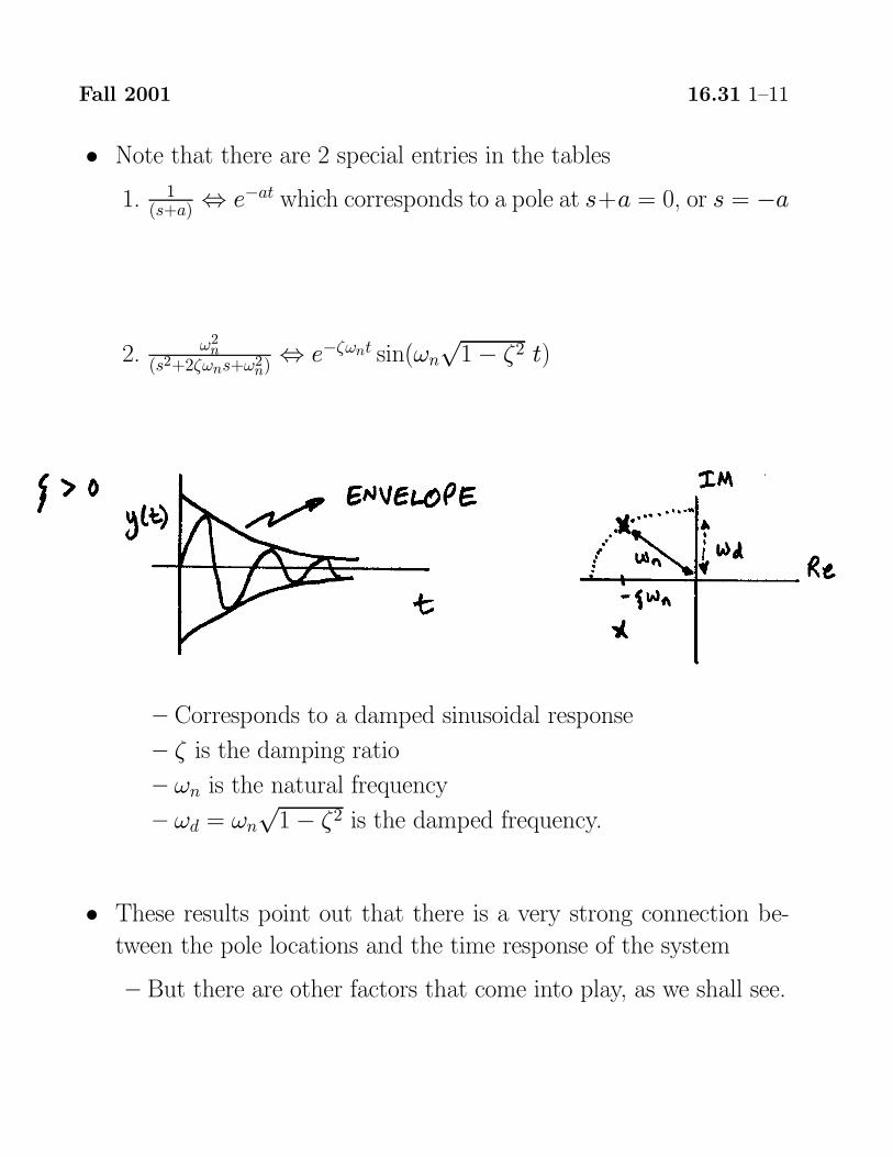
• Note that there are 2 special entries in the tables

1. 1(s+a) ⇔ e−at which corresponds to a pole at s+a = 0, or s = −a

2. ω2n(s2+2ζωns+ω2n)

⇔ e−ζωnt sin(ωn√1− ζ2 t)

— Corresponds to a damped sinusoidal response

— ζ is the damping ratio

— ωn is the natural frequency

— ωd = ωn√1− ζ2 is the damped frequency.

• These results point out that there is a very strong connection be-

tween the pole locations and the time response of the system

— But there are other factors that come into play, as we shall see.

Fall 2001 16.31 1—12

• For a second order system, we can be more explicit and relate the

main features of the step response (time) and the pole locations

(frequency domain).

G(s) =ω2n

(s2 + 2ζωns + ω2n)

with u(t) a step, so that u(s) = 1/s

• Then y(s) = G(s)u(s) = ω2ns(s2+2ζωns+ω2n)

which gives (σ = ζωn)

y(t) = 1− e−σtcos(ωdt) + σ

ωdsin(ωdt)

• Several key time domain features:

— Rise time tr (how long to get close to the final value?)

— Settling time ts (how long for the transients to decay?)

— Peak overhsoot Mp, tp (how far beyond the final value does the

system respond, and when?)

• Can analyze the system response to determine that:

1. tr ≈ 2.2/whwh = wn 1− 2ζ2 + 2− 4ζ2 + 4ζ4 1/2

or can use tr ≈ 1.8/wn2. ts(1%) = 4.6/(ζωn)

3. Mp = e

−πζ√1−ζ2 and tp = π/ωd

• Formulas relate time response to pole locations. Can easily evalute

if the closed-loop system will respond as desired.

— Use to determine acceptable locations for closed-loop poles.

Fall 2001 16.31 1—13

• Examples:

— Max rise time - min ωn

— Max settling time — min σ = ζωn

— Max overshoot — min ζ

• Usually assume that the response of more complex systems (i.e.

ones that have more than 2 poles) is dominated by the lowest

frequency pole pair.

— Then the response is approximately second order, but we

must check this

• These give us a good idea of where we would like the closed-loop

poles to be so that we can meet the design goals.

— Feedback control is all about changing the location of the system

poles from the open-loop locations to the closed-loop ones.

— This course is about a new way to do these control designs

Please refer to the “Design Aids” section of: Franklin, Gene F., Powell, J. David and Abbas Emami-Naeini. 1994. Feedback Control of Dynamic Systems – 3rd Ed. Addison-Wesley