Learning to relate images: Mapping units,complex cells and simultaneous eigenspaces

Roland MemisevicUniversity of Frankfurtro@cs.uni-frankfurt.de

April 5, 2012

Abstract

A fundamental operation in many vision tasks, including motion understand-ing, stereopsis, visual odometry, or invariant recognition, is establishing corre-spondences between images or between images and data from other modalities.We present an analysis of the role that multiplicative interactions play in learn-ing such correspondences, and we show how learning and inferring relationshipsbetween images can be viewed as detecting rotations in the eigenspaces sharedamong a set of orthogonal matrices. We review a variety of recent multiplicativesparse coding methods in light of this observation. We also review how the squar-ing operation performed by energy models and by models of complex cells can bethought of as a way to implement multiplicative interactions. This suggests thatthe main utility of including complex cells in computational models of vision maybe that they can encode relations not invariances.

1 Introduction

Correspondence is arguably the most ubiquitous computational primitive in vision:Tracking amounts to establishing correspondences between frames; stereo visionbetween different views of a scene; optical flow between any two images; invariantrecognition between images and invariant descriptions in memory; odometry betweenimages and motion information; action recognition between frames; etc. In these andmany other tasks, the relationship between images not the content of a single imagecarries the relevant information. Representing structures within a single image, such ascontours, can be also considered as an instance of a correspondence problem, namelybetween areas, or pixels, within an image1. The fact that correspondence is such acommon operation across vision suggests that the task of representing relations may

1The importance of image correspondence in action understanding is nicely illustrated in Heiderand Simmel’s 1944 video of geometric objects engaged in various “social activities” [15] (althouth the

1

arX

iv:s

ubm

it/04

4812

8 [

cs.C

V]

5 A

pr 2

012

have to be kept in mind when trying to build autonomous vision systems and whentrying to understand biological vision.

A lot of progress has been made recently in building models that learn to solvetasks like object recognition from independent, static images. One of the reasons for therecent progress is the use of local features, which help virtually eliminate the notoriouslydifficult problems of occlusions and small invariances. A central finding is that the rightchoice of features not the choice of high-level classifier or computational pipeline arewhat typically makes a system work well. Interestingly, some of the best performingrecognition models are highly biologically consistent, in that they are based on featuresthat are learned unsupervised from data. Besides being biological plausible, featurelearning comes with various benefits, such as helping overcome tedious engineering,helping adapt to new domains and allowing for some degree of end-to-end learning inplace of constructing, and then combining, a large number of modules to solve a task.The fact that tasks like object recognition can be solved using biologically consistent,learning based methods raises the question whether understanding relations can beamenable to learning in the same way. If so, this may open up the road to learningbased and/or biologically consistent approaches to a much larger variety of problemsthan static object recognition, and perhaps also beyond vision.

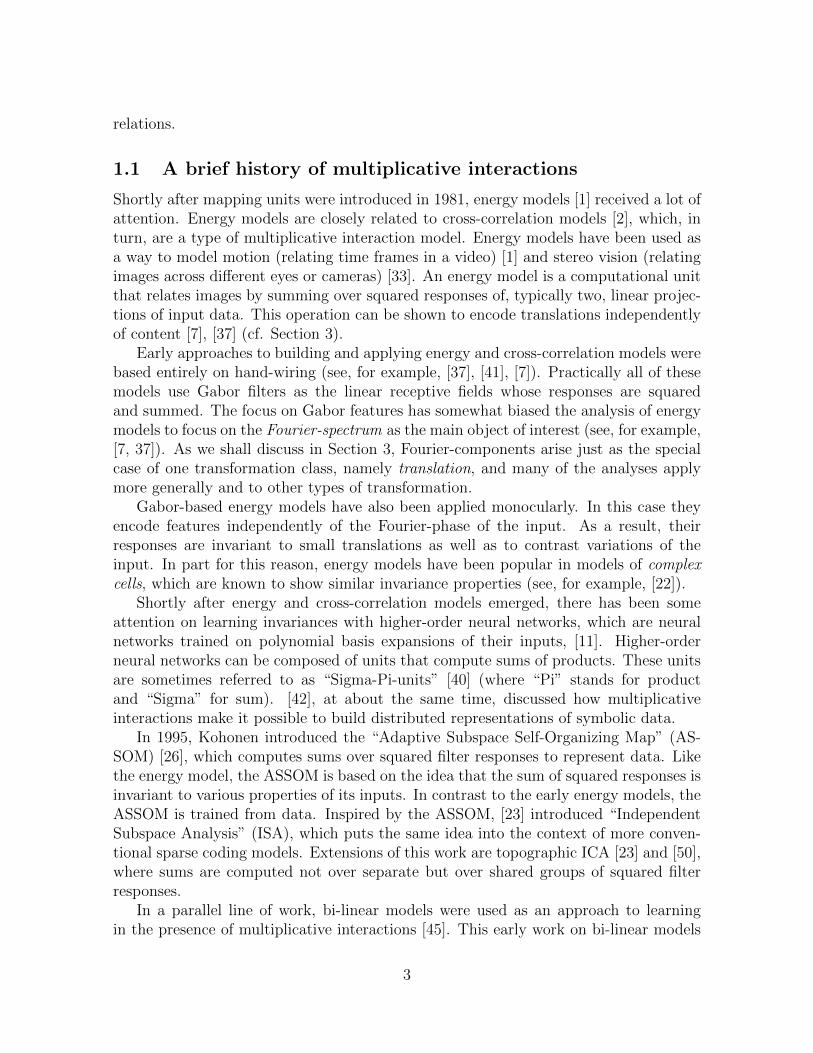
In this paper, we review a variety of recent methods that address correspondencetasks by learning local features. We discuss how the common computational principlebehind all these methods are multiplicative interactions, which were introduced to thevision community 30 years ago under the terms “mapping units” [18] and “dynamicmappings” [48]. An illustration of mapping units is shown in Figure 1: The three vari-ables shown in the figure interact multiplicatively, and as a result, each variable (say, zk)can be thought of as dynamically modulating the connections between other variablesin the model (xi and yj). Likewise, the value of any variable (eg., yj) can be thoughtof as depending on the product of the other variables (xi, zk) [18]. This is in contrastto common feature learning models like ICA, Restricted Boltzmann Machines, auto-encoder networks and many others, all of which are based on bi-partite networks, thatdo not involve any three-way multiplicative interactions. In these models, independenthidden variables interact with independent observable variables, such that the value ofany variable depends on a weighted sum not product of the other variables. Closelyrelated to models of mapping units are energy models (for example, [1]), which may bethought of as a way to “emulate” multiplicative interactions by computing squares.

We shall show how both mapping units and energy models can be viewed as ways tolearn and detect rotations in a set of shared invariant subspaces of a set of commutingmatrices. Our analysis may help understand why action recognition methods seem toprofit from squaring non-linearities (for example, [27]), and it predicts that squaringand cross-products will be helpful, in general, in applications that involve representing

original intent of that video goes beyond making a case for correspondences). Each single frame depictsa rather meaningless set of geometric objects and conveys almost no information about the content ofthe movie. The only way to understand the movie is by understanding the motions and actions, andthus by decoding the relationships between frames.

2

relations.

1.1 A brief history of multiplicative interactions

Shortly after mapping units were introduced in 1981, energy models [1] received a lot ofattention. Energy models are closely related to cross-correlation models [2], which, inturn, are a type of multiplicative interaction model. Energy models have been used asa way to model motion (relating time frames in a video) [1] and stereo vision (relatingimages across different eyes or cameras) [33]. An energy model is a computational unitthat relates images by summing over squared responses of, typically two, linear projec-tions of input data. This operation can be shown to encode translations independentlyof content [7], [37] (cf. Section 3).

Early approaches to building and applying energy and cross-correlation models werebased entirely on hand-wiring (see, for example, [37], [41], [7]). Practically all of thesemodels use Gabor filters as the linear receptive fields whose responses are squaredand summed. The focus on Gabor features has somewhat biased the analysis of energymodels to focus on the Fourier-spectrum as the main object of interest (see, for example,[7, 37]). As we shall discuss in Section 3, Fourier-components arise just as the specialcase of one transformation class, namely translation, and many of the analyses applymore generally and to other types of transformation.

Gabor-based energy models have also been applied monocularly. In this case theyencode features independently of the Fourier-phase of the input. As a result, theirresponses are invariant to small translations as well as to contrast variations of theinput. In part for this reason, energy models have been popular in models of complexcells, which are known to show similar invariance properties (see, for example, [22]).

Shortly after energy and cross-correlation models emerged, there has been someattention on learning invariances with higher-order neural networks, which are neuralnetworks trained on polynomial basis expansions of their inputs, [11]. Higher-orderneural networks can be composed of units that compute sums of products. These unitsare sometimes referred to as “Sigma-Pi-units” [40] (where “Pi” stands for productand “Sigma” for sum). [42], at about the same time, discussed how multiplicativeinteractions make it possible to build distributed representations of symbolic data.

In 1995, Kohonen introduced the “Adaptive Subspace Self-Organizing Map” (AS-SOM) [26], which computes sums over squared filter responses to represent data. Likethe energy model, the ASSOM is based on the idea that the sum of squared responses isinvariant to various properties of its inputs. In contrast to the early energy models, theASSOM is trained from data. Inspired by the ASSOM, [23] introduced “IndependentSubspace Analysis” (ISA), which puts the same idea into the context of more conven-tional sparse coding models. Extensions of this work are topographic ICA [23] and [50],where sums are computed not over separate but over shared groups of squared filterresponses.

In a parallel line of work, bi-linear models were used as an approach to learningin the presence of multiplicative interactions [45]. This early work on bi-linear models

3

zk

xi

yj

Figure 1: Symbolic representation of a mapping unit [18]. The triangle symbolizesmultiplicative interactions between the three variables zk, xi and yj. The value of anyone of the three variables is a function of the product of all the others. ([18]).

used these as global models trained on whole images rather than using local receptivefields. In contrast to more recent approaches to learning with multiplicative interac-tions, training typically involved filling a two-dimensional grid with data that shows twotypes of variability (sometimes called “style” and “content”). The purpose of bi-linearmodels is then to untangle the two degrees of freedom in the data. More recent workdoes not make this distinction, and the purpose of multiplicative hidden variables ismerely to capture the multiple ways in which two images can be related. [13], [36], [30],for example, show how multiplicative interactions make it possible to model the multi-tude of relationships between frames in natural videos. [30] also show how they allowus to model more general classes of relations between images. An earlier multiplicativeinteraction model, that is also related to bi-linear models, is the “routing-circuit” [35].

Multiplicative interactions have also been used to model structure within staticimages, which can be thought of as modeling higher-order relations, and, in particular,pair-wise products, between pixel intensities (for example, [25, 23, 49, 21, 38, 6, 29]).

Recently, [32] showed how multiplicative interactions between a class-label and afeature vector can be viewed as an invariant classifier, where each class is representedby a manifold of allowable transformations. This work may be viewed as a modernversion of the model that introduced the term mapping units in 1981 [18]. The maindifference between 2011 and 1981 is that models are now trained from large datasets.

2 Learning to relate images

2.1 Feature learning

We briefly review standard feature learning models in this section and we discuss rela-tional feature learning in Section 2.2. We discuss extensions of relational models andhow they relate to complex cells and to energy models in Section 3.

Practically all standard feature learning models can be represented by a graphicalmodel like the one shown in Figure 2.1 (a). The model is a bi-partite network thatconnects a set of unobserved, latent variables zk with a set of observable variables (for

4

yj

z

wjk

zk

y

zk

yj

wkj

ajk

y

y

yj

(a) (b)

Figure 2: (a) Sparse coding graphical model. (b) Auto-encoder network.

example, pixels) yj. The weights wjk, which connect pixel yj with hidden unit zk,are learned from a set of training images {yα}α=1,...,N . The vector of latent variablesz = (zk)k=1...K in Figure 2.1 (a) is considered to be unobserved, so one has to inferit, separately for each training case, along with the model parameters for training.The graphical model shown in the figure represents how the dependencies betweencomponents yi and zk are parameterized, but it does not define a model or learningalgorithm. A large variety of models and learning algorithms can be parameterized asin the figure, including principal components, mixture models, k-means clustering, orrestricted Boltzmann machines [16]. Each of these can in principle be used as a featurelearning method (see, for example, [5] for a recent quantitative comparison).

For the hidden variables to extract useful structure from the images, their capacityneeds to be constrained. The simplest form of constraining it is to let the dimensionalityK be smaller than the dimensionality J of the images. Learning in this case amountsto performing dimensionality reduction. It has become obvious recently that it is moreuseful in most applications to use an over-complete representation, that is, K > J ,and to constrain the capacity of the latent variables instead by forcing the hidden unitactivities to be sparse. In Figure 2.1, and in what follows, we use K < J to symbolizethe fact that z is capacity-constrained, but it should be kept in mind that capacitycan be (and often is) constrained in other ways. The most common operations in themodel, after training, are: “Inference” (or “Analysis”): Given image y, compute z; and“Generation” (or “Synthesis”): Invent a latent vector z, then compute y.

A simple way to train a model, given training images, is by minimizing reconstruc-tion error combined with a sparsity encouraging term for the hidden variables (for

5

example, [34]): ∑α

(‖yα −

∑k

zαkW.k‖2 + λ|zαk |)

(1)

Optimization is with respect to both W = (wjk)j=1...J,k=1...K and all zα. For this end,it is common to alternate between optimizing W and optimizing all zα. After training,inference then amounts to minimizing the same expression for test images (with Wfixed).

To avoid iterative optimization during inference, one can eliminate z by defining itimplicitly as a function of y. A common choice of function is z = σ (Ay) where A isa matrix and σ(·) is a squashing non-linearity, such as σ(a) = (1 + exp(−a))−1, whichconfines the values of z to reside in a fixed interval. This model is the well-knownauto-encoder (for example, [47]) and it is depicted in Figure 2.1. Learning amountsto minimizing reconstruction error with respect to both A and W . In practice, it iscommon to enforce A := WT in order to reduce the number of parameters and forconsistency with other sparse coding models.

One can add a penalty term that encourages sparsity of the latent variables. Al-ternatively, one can train auto-encoders, such that they de-noise corrupted version oftheir inputs, which can be achieved by simply feeding in corrupted inputs during train-ing (but measuring reconstruction error with respect to the original data). This turnsauto-encoders into “de-noising auto-encoders” [47], which show properties similar toother sparse coding methods, but inference, like in a standard auto-encoder, is a simplefeed-forward mapping.

A technique similar to the auto-encoder is the Restricted Boltzmann machine (RBM):RBMs define the joint probability distribution

p(y, z) =1

Zexp

(∑jk

wjkyjzk), (2)

from which one can derive

p(zk|y) = sigmoid(∑

j

wjkyj)

and p(yj|z) = sigmoid(∑

j

wjkzk), (3)

showing that inference, again, amounts to a linear mapping plus non-linearity. Learningamounts to maximizing the average log-probability 1

N

∑α log p(yα) of the training data.

Since the derivatives with respect to the parameters are not tractable (due to thenormalizing constant Z in Eq. 2), it is common to use approximate Gibbs samplingin order to approximate them. This leads to a Hebbian-like learning rule known ascontrastive divergence training [16].

Another common sparse coding method is independent components analysis(ICA) (for example, [22]). One way to train an ICA-model that is complete (that is,where z has the same size as y) is by encouraging latent responses to be sparse, while

6

preventing weights from becoming degenerate [22]:

minW‖WTy‖1 (4)

s.t. WTW = I (5)

Enforcing the constraint can be inefficient in practice, since it requires an eigen decom-position.

For most feature learning models, inference and generation are variations of the twolinear mappings:

zk =∑j

wjkyj (6)

yj =∑k

wjkzk (7)

The set of model parameters W·k for any k are typically referred to as “features” or“filters” (although a more appropriate term would be “basis functions”; we shall usethese interchangeably). Practically all methods yield Gabor-like features when trainedon natural images. An advantage of non-linear models, such as RBM’s and auto-encoders, is that stacking them makes it possible to learn feature hierarchies (“deeplearning”) [17].

In practice, it is common to add bias terms, such that inference and generation(Eqs. 6 and 7) are affine not linear functions, for example, yj =

∑k wjkzk + bj for

some parameter bj. We shall refrain from adding bias terms to avoid clutter, notingthat, alternatively, one may think of y and z as being in “homogeneous” coordinates,containing an extra, constant 1-dimension.

Feature learning is typically performed on small images patches of size betweenaround 5× 5 and 50× 50 pixels. One reason for this is that training and inference canbe computationally demanding. More important, local features make it possible to dealwith images of different size, and to deal with occlusions and local object variations.Given a trained model, two common ways to perform invariant recognition on testimages are:

“Bag-Of-Features”: Crop patches around interest points (such as SIFT or Harriscorners), compute latent representation z for each patch, collapse (add up) all represen-tations to obtain a single vector zImage, classify zImage using a standard classifier. Thereare several variations of this scheme, including using an extra clustering-step beforecollapsing features, or using a histogram-similarity in place of Euclidean distance forthe collapsed representation.

“Convolutional”: Crop patches from the image along a regular grid; compute zfor each patch; concatenate all descriptors into a very large vector zImage; classify zImage

using a standard classifier. One can also use combinations of the two schemes (see, forexample [5]).

Local features yield highly competitive performance in object recognition tasks (forexample, [5]). In the next section we discuss recent approaches to extending featurelearning to encode relations between, as opposed to content within, images.

7

?

yx

z

Figure 3: Learning to encode relations: We consider the task of learning latent variablesz that encode the relationship between images x and y, independently of their content.

2.2 Encoding relations

We now consider the task of learning relations between two images x and y as illus-trated2 in Figure 3, and we discuss the role of multiplicative interactions when learningrelations.

2.2.1 The need for multiplicative interactions

A naive approach to modeling relations between two images would be to perform sparsecoding on the concatenation. A hidden unit in such a model would receive as input thesum of two projections, one from each image. To detect a particular transformation, thetwo receptive fields would need to be defined, such that one receptive field is the othermodified by the transformation that the hidden unit is supposed to detect. The netinput that the hidden unit receives will then tend to be high for image pairs showingthe transformation. However, the net input will equally dependent on the imagesthemselves. The reason is that hidden variables are akin to logical “OR”-gates, whichaccumulate evidence (see, for example [51] for a discussion).

It is straightforward to build a content-independent detector if we allow for multi-plicative interactions between the variables. In particular, consider the outer productL := xyT between two one-dimensional, binary images, as shown in Figure 4. Everycomponent Lij of this matrix constitutes evidence for exactly one type of transforma-

2Face images taken from the data-base described in [46]

8

zk

wijk

(a) (b) (c)

Figure 4: (a) The diagonal of L := xyT contains evidence for the identity transforma-tion. (b) The secondary diagonals contain evidence for shifts. (c) A hidden unit thatpools over one of the diagonals can detect transformations. This hidden unit computesa sum over products.

tion (translation, in the example). The components Lij act like AND-gates, that candetect coincidences. Since a component Lij is equal to 1 only when both correspondingpixels are equal to 1, a hidden unit that pools over multiple components (Figure 4 (c))is much less likely to receive spurious activity that depends on the image content ratherthan on the transformation. Note that pooling over the components of L amounts tocomputing the correlation of the output image with a transformed version of the inputimage. The same is true for real-valued data.

Based on these observations, a variety of sparse coding models were suggested whichencode transformations (for example, [36, 13, 30]). The number of parameters is typi-cally equal to (the number of hidden variables) × (the number of input-pixels) × (thenumber of output pixels). It is instructional to think of the parameters as populatinga 3-way-“tensor” w with components wijk.

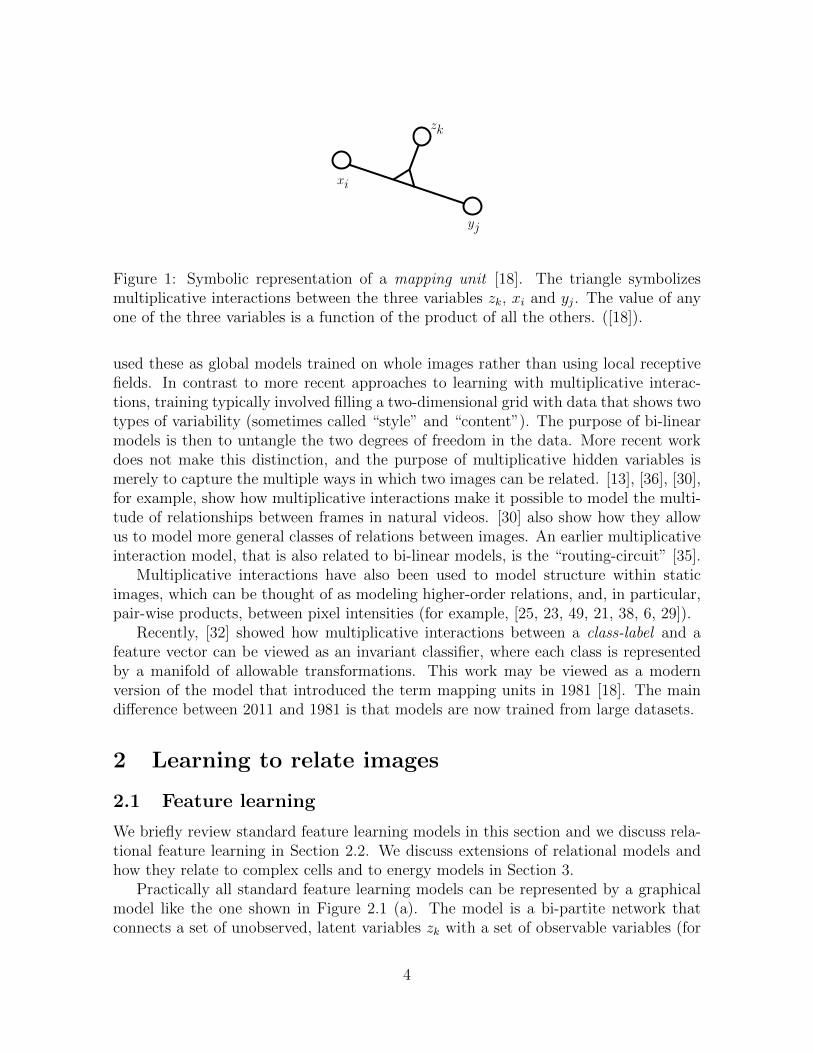
Figure 5 (left) shows two alternative illustrations of this type of model (adaptedfrom [30]). Sub-figure (a) shows that each hidden variable can blend in a slice w··kof the parameter tensor. Each slice is a matrix connecting each input pixel to eachoutput-pixel. We can think of this matrix as performing linear regression in the spaceof stacked gray-value intensities, known commonly as a “warp”. Thus, the model as awhole can be thought of as defining a factorial mixture of warps.

Alternatively, each input pixel can be thought of as blending in a slice wi·· of theparameter tensor. Thus, we can think of the model as a standard sparse coding modelon the output image (Figure 5 (left)), whose parameters are modulated by the inputimage. This turns the model into a predictive or conditional sparse coding model[36, 30]. In both cases, hidden variables take on the roles of dynamic mapping units[18, 48] which encode the relationship not the content of the images. Each unit in themodel can gate connections between other variables in the model. We shall refer to thistype of model as “gated sparse coding”, or synonymously as “cross-correlation model”.

Like in a standard sparse coding model one needs to include biases in practice. Theset of model parameters thus consists of the three-way parameters wijk, as well as ofsingle-node parameters wi, wj and wk. One could also include “higher-order-biases”[30] like wik, which connect two groups of variables, but it is not common to do so. Likebefore, we shall drop all bias terms in what follows in order to avoid clutter. Both simple

9

yjxi

zk

z

x y

yj

xi

x y

z

zk

Figure 5: Relating images using multiplicative interactions. Two equivalent views ofthe same type of model.

biases and higher-order biases can be implemented by adding constant-1 dimensions todata and to hidden variables.

2.3 Inference

The graphical model of gated sparse coding models is tri-partite. That of a standardsparse coding model is bi-partite. Inference can be performed in almost the same asin a standard sparse coding model, whenever two out of three groups of variables havebeen observed.

Consider, for example, the task of inferring z, given x and y (see Figure 6 (a)). Re-call that for a standard sparse coding model, we have: zk =

∑j wjkyj (up to component-

wise non-linearities). It is instructional to think of the gated sparse coding model asturning the weights into a function of x. If that function is linear: wjk(x) =

∑iwijkxi,

we get:

zk =∑j

wjkyj =∑j

(∑i

wijkxi)yj =

∑ij

wijkxiyj (8)

which is exactly of the form discussed in the previous section.Eq. 8 shows that inference amounts to computing for each output-component yj a

quadratic form in x and z defined by the weight tensor w·j·. Considering either x or zas fixed, one can also think of inference as a simple linear function like in a standardsparse coding model. This property is typical of models with bi-linear dependencies[45]. Despite the similarity to a standard sparse coding model, the meaning of inferencediffers from standard sparse coding: The meaning of z, here, is the transformation thattakes x to y (or vice versa).

10

yj

xi

x y

z

zk

yj

xi

x y

z

zk

(a) (b)

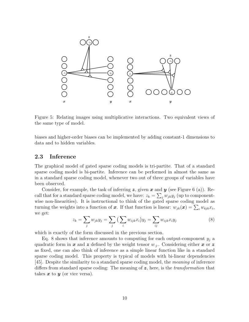
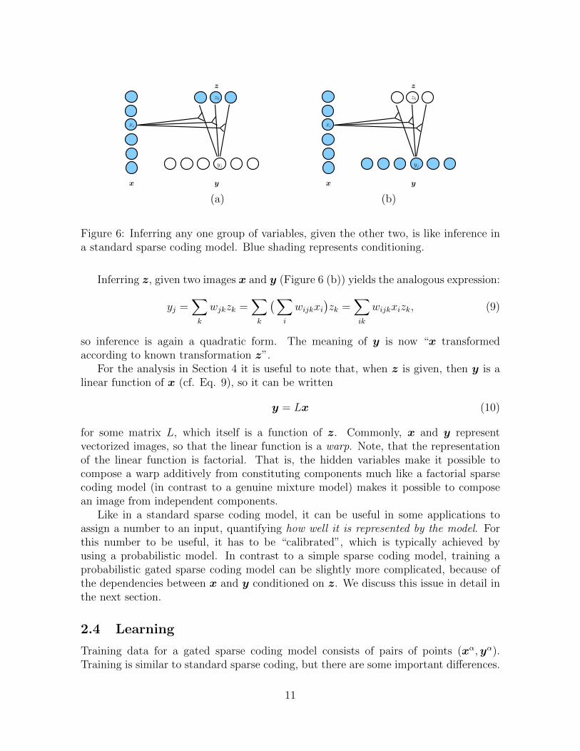
Figure 6: Inferring any one group of variables, given the other two, is like inference ina standard sparse coding model. Blue shading represents conditioning.

Inferring z, given two images x and y (Figure 6 (b)) yields the analogous expression:

yj =∑k

wjkzk =∑k

(∑i

wijkxi)zk =

∑ik

wijkxizk, (9)

so inference is again a quadratic form. The meaning of y is now “x transformedaccording to known transformation z”.

For the analysis in Section 4 it is useful to note that, when z is given, then y is alinear function of x (cf. Eq. 9), so it can be written

y = Lx (10)

for some matrix L, which itself is a function of z. Commonly, x and y representvectorized images, so that the linear function is a warp. Note, that the representationof the linear function is factorial. That is, the hidden variables make it possible tocompose a warp additively from constituting components much like a factorial sparsecoding model (in contrast to a genuine mixture model) makes it possible to composean image from independent components.

Like in a standard sparse coding model, it can be useful in some applications toassign a number to an input, quantifying how well it is represented by the model. Forthis number to be useful, it has to be “calibrated”, which is typically achieved byusing a probabilistic model. In contrast to a simple sparse coding model, training aprobabilistic gated sparse coding model can be slightly more complicated, because ofthe dependencies between x and y conditioned on z. We discuss this issue in detail inthe next section.

2.4 Learning

Training data for a gated sparse coding model consists of pairs of points (xα,yα).Training is similar to standard sparse coding, but there are some important differences.

11

In particular, note that the gated model is like a sparse coding model whose input isthe vectorized outer-product xyT (cf. Section 2.2), so that standard learning criteria,such as squared error, are obviously not appropriate.

2.4.1 Predictive training

One way to train the model is utilizing the view as predictive sparse coding (Figure 6(b)), and to train the model conditionally by predicting y given x [13], [36], [30].

Recall that we can think of the inputs x as modulating the parameters. Thismodulation is case-dependent. Learning can therefore be viewed as “sparse coding withcase-dependent weights”. The cost that data-case (xα,yα) contributes is:∑

j

(yαj −

∑ik

wijkxαi z

αk )2 (11)

Differentiating with respect to wijk is the same as in a standard sparse coding model.In particular, the model is still linear wrt. the parameters. Predictive learning istherefore possible with gradient-based optimization similar to standard feature learning(cf. Section 2.1).

To avoid iterative inference, it is possible to adapt various sparse coding variants,like auto-encoders and RBMs (Section 2.1) to the conditional case. As an example, weobtain a “gated Boltzmann machine” (GBM) by changing the energy function into thethree-way energy [30]:

E(x,y, z) =∑ijk

wijkxiyjzk (12)

and exponentiating and normalizing:

p(y, z|x) =1

Z(x)exp

(E(x,y, z)

), Z(x) =

∑y,z

exp(E(x,y, z)

)(13)

Note that the normalization is over y and z only, which is consistent with our goalof defining a predictive model. It is possible to define a joint model, but this makestraining more difficult (cf. Section 2.4.2). Like in a standard RBM, training involvessampling z and y. In the relational RBM samples are drawn from the conditionaldistributions p(y|z,x) and p(z|y,x).

As another example, we can turn an auto-encoder into a relational auto-encoder, bydefining the encoder and decoder parameters A and W as linear functions of x ([28],[29]). Learning is then essentially the same as in a standard auto-encoder modelingy. In particular, the model is still a directed acyclic graph, so one can use simpleback-propagation to train the model. See Figure 7 for an illustration.

2.4.2 Symmetric training

In probabilistic terms, predictive training amounts to modeling the conditional distri-bution p(y|x) =

∫zp(y, z|x) dz. [43] show how modeling instead the joint distribution

12

xizk

yj y

yj y

xz

(a) (b)

Figure 7: (a) Relational auto-encoder. (b) Toy data commonly used to test relationalmodels. There is no structure in the images, only in their relationship.

can make it possible to perform image matching, by allowing us to quantify how com-patible any two images are under to the trained model.

Formally, modeling the joint amounts simply to changing the normalization constantof the three-way RBM to Z =

∑x,y,z exp

(E(x,y, z)

)(cf. previous section). Learning

is more complicated, however, because the simplifying view of case-based modulationno longer holds. [43] suggest using three-way Gibbs sampling to train the model.

As an alternative to modeling a joint probability distribution, [29] show how onecan instead use a relational auto-encoder trained symmetrically on the sum of the twopredictive objectives∑

j

(yαj −

∑ik

wijkxαi z

αk )2 +

∑i

(xαi −

∑jk

wijkyαj z

αk )2 (14)

This forces parameters to be able to transform in both directions, and it can giveperformance similar to symmetrically trained, fully probabilistic models [29]. Like anauto-encoder, this model can be trained with gradient based optimization.

2.4.3 Learning higher-order within-image structure

Another reason for learning the joint distribution is that it allows us to model higher-order within-image structure (for example, [25, 39, 23]).

[39] apply a GBM to the task of modeling second-order within-image features, thatis, features that encode pair-wise products of pixel intensities. They show that this canbe achieved by optimizing the joint GBM distribution and using the same image asinput x and as output y. In contrast to [43], [39] suggest hybrid Monte Carlo to trainthe joint.

One can also combine higher-order models with standard sparse coding models, by

13

using some hidden units to model higher-order structure and some to learn linear codes[38, 29].

2.4.4 Toy example: Motion extraction and analogy making

Figure 8 (a) shows a toy example of a gated Boltzmann machine applied to translations.The model was trained on images showing iid random dots where the output image y isa copy of the input image x shifted in a random direction. The center column in bothplots in Figure 8 visualizes the inferred transformation as a vector field. The vector-field was produced by (i) inferring the transformation given the image pair (Eq. 8),(ii) computing the transformation from the inferred hiddens, and (iii) finding for eachinput-pixel the output-position it is most strongly connected to [30]. The two right-most columns in both plots show how the inferred transformation can be applied to newimages by analogy, that is, by computing the output-image given a new input imageand the inferred transformation (Eq. 9). Figure 8 (b) shows an example, where thetransformations are split-screen translations, that is, translations which are independentin the top half vs. the bottom half of the image. This illustrates how the model has todecompose transformations into factorial constituting transformations.

3 Factorization and energy models

In the following, we discuss the close relationship between gated sparse coding modelsand energy models. For this end, we first describe how parameter factorization makesit possible to pre-process input images and thereby reduce the number of parameters.

3.1 Factorizing the gating parameters

The number of gating parameters is roughly cubic in the number of pixels, if we assumethat the number of constituting transformations is about the same as the number ofpixels. It can easily be more for highly over-complete hiddens. [31] suggest reducingthat number by factorizing the parameter tensor W into three matrices, such that eachcomponent wijk is given by the “three-way inner product”

wijk =∑ijk

F∑f=1

wxifwyjfw

zkf (15)

Here, F is a number of hidden “factors”, which, like the number K of hidden units, hasto be chosen by hand or by cross-validation. The matrices wx, wy and wz are I × F ,J × F and K × F , respectively.

An illustration of this factorization is given in Figure 9 (a). It is interesting tonote that, under this factorization, the activity of output-variable yj, by using the

14

(a) (b)

Figure 8: Inferring motion direction from test data. (a) Coherent motion across thewhole image. (b) “Factorial motion” that is independent in different image regions. Inboth plots, the meaning of the five columns is as follows (left-to-right): Random testimages x, random test images y, inferred flow-field, new test-image x, inferred outputy.

15

wyjf

wxif

wzkf

wijk

x y

xi yj

z

zk

(a) (b)

Figure 9: (a) Factorizing the parameter tensor. (b) Interpreting factorization as filtermatching.

distributive law, can by written:

yj =∑ik

wijkxizk =∑ik

(∑f

wxifwyjfw

zkf )xizk =

∑f

wyjf (∑i

wxifxi)(∑k

wzkfzk) (16)

Similarly, for zk we have

zk =∑ij

wijkxiyj =∑ij

(∑f

wxifwyjfw

zkf )xiyj =

∑f

wzkf (∑i

wxifxi)(∑j

wyjfyj) (17)

One can obtain a similar expression for the energy in a gated Boltzmann machine. Eq.17 shows that factorization can be viewed as filter matching : For inference, each groupof variables x, y and z are projected onto linear basis functions which are subsequentlymultiplied, as illustrated in Figure 9 (b).

It is important to note that the way factorization reduces parameters is not byprojecting data onto a lower-dimensional space before computing the multiplicativeinteractions – a claim that can be found frequently in the literature. In fact, frequently,F is chosen to be larger than I and/or J . The way that factorization reduces the numberof parameters is by restricting three-way connectivity. Learning then amounts to findingbasis functions that can deal with this restriction optimally. Using the factorizationin Eq. 15 amounts to allowing each factor to engage only in a single multiplicativeinteraction.

All gated sparse coding models can be subjected to this factorization. Trainingis similar to training an unfactored model by using the chain rule and differentiatingEq. 15. An example of a factored gated auto-encoder is described in [29]. Virtuallyall factored models that were introduced use the restriction of single multiplicativeinteractions (Eq. 15). An open research question is to what degree a less restrictive

16

connectivity – equivalently, using a non-diagonal core-tensor in the factorization – wouldbe advantageous.

[31] show empirically how training factored model leads to filter-pairs that optimallyrepresent transformation classes, such as Fourier-components for translations and apolar variant of Fourier-components for rotations. Figures 10 and 11 show examples offilters learned from translations, affine transformations, split-screen translations, whichare independent in the top and bottom half of the image, and natural video. For trainingthe filters in the top rows and on the bottom right, we used data-sets described in [31]and [29] and the model described in [29]. The filters resemble receptive fields foundin various cells in visual cortex [10]. To obtain split-screen filters (bottom left) wegenerated a data-set of split-screen translations and trained the model described in[31]. In Section 4, we provide an analysis that sheds some light onto why the filterstake on this form.

3.2 Energy models

Energy models [1, 33] are an alternative approach to modeling image motion and dis-parities, and they have been deployed monocularly, too. A main application of energymodels is the detection of small translational motion in image pairs. This makes themsuitable as biologically plausible mechanisms of both local motion estimation and binoc-ular disparity estimation. Energy models detect motion by projecting two images ontotwo phase-shifted Gabor functions each (for a total of four basis function responses).The two responses across the images are added and squared. The sum of these twosquared, spatio-temporal responses then yields the response of the energy model.

The rationale behind the energy model is that, since each within-image Gabor filterpair can be thought of as a localized spatio-temporal Fourier component, the sum of thesquared components yields an estimate of spectral energy, which is not dependent of thephase – and thus to a large degree not dependent on the content – of the input images.The two filters within each image need to be sine/cosine pairs, which is commonlyreferred to as being “in quadrature”.

A detector of local shift can be built by using a set of energy models tuned todifferent frequencies. To turn the set of energy responses into an estimate of localtranslation, one can, for example, pick the model with the strongest response [41, 37],or use pooling to get a more stable estimate [7].

[26, 23] suggest learning energy-like models from data by extending a sparse codingmodel with an elementwise squaring operation, followed by a linear pooling layer. Incontrast to the original energy model, one may use more than exactly two filters to poolover, and pooling weights may be learned along with basis functions, instead of beingfixed to be 1. Figure 12 shows an illustration of this type of model applied to an imagepair. As the figure shows, this type of model can be viewed as a two-layer network,with a hidden layer that uses an elementwise squaring nonlinearity.

For learning, [23] suggest adopting ICA by forcing the responses of latent variables(which are now sums of squared basis function responses) to be sparse, while keeping the

17

Figure 10: Input filters learned from various types of transformation. Top-left: Transla-tion, Top-right: Rotation, Bottom-left: split-screen translation, Bottom-right: Naturalvideos. See figure 11 on the next page for corresponding output filters.

filters orthogonal to avoid degenerate solutions, just like when training a standard ICAmodel (cf. Section 2.1). This approach is known as “Independent Subspace Analysis”(ISA). We shall refer to the hidden layer nodes as “factors” in analogy to the hiddenlayer of a factored GBM. Both ISA and factored gated Boltzmann machines were shownto yield state-of-the-art performance in various motion recognition tasks [27, 44].

18

Figure 11: Output filters learned from various types of transformation. Top-left: Trans-lation, Top-right: Rotation, Bottom-left: split-screen translation, Bottom-right: Natu-ral videos. See figure 10 on the previous page for corresponding input filters.

3.3 Relationship between gated sparse coding and energy mod-els

Learning energy models, such as ISA, on the concatenation of two inputs x and y isclosely related to learning gated sparse coding models. Let wx·f (wy·f ) denote the set ofweights connecting part x (y) of the concatenated input with factor f (cf. Figure 12).

19

zk

z

wzkf

x y

xi yj

(·)2

wyjfwx

if

Figure 12: Illustration of Independent Subspace Analysis applied to an image pair(x,y).

The activity of hidden unit zk in an energy model is given by

zk =∑f

wzkf(wx·f

Tx + wy·fTy)2

(18)

=∑f

wzkf(2(wx·f

Tx)(wy·fTy) + (wx·f

Tx)2 + (wy·fTy)2

)(19)

Up to the quadratic terms in Eq. 19, hidden unit activities are the same as in a gatedsparse coding model. As we shall discuss in detail below, the quadratic terms do nothave a significant effect on the meaning of the hidden units. They can therefore alsobe thought of as a way to implement mapping units that encode relations.

3.4 Implementing gated sparse coding models

Over the years, a variety of tricks and recipes have emerged, which can simplify, stabi-lize, or speed up, learning in the presence of multiplicative interactions. One approach,that is used by practically everyone in the field, is to normalize output filter matriceswx and wy during learning, such that all filter wx·f and wy·f grow slowly and maintainroughly the same length as learning progresses. A common way to achieve this is tomaintain a running average of the average norm of the filters during learning and tore-normalize each filter to have this norm after every learning update. Furthermore, itis common to connect top-level hidden units locally to the factors, rather than usingfull connectivity. The theoretical discussion in the next section provides some intuition

20

into why local connectivity helps speed up learning. A slightly more complicated ap-proach is to let all hidden units populate a virtual “grid” in a low-dimensional space(for example, 2-D) and to connect hidden units to factors, such that neighboring hiddenunits are connected to the same or to overlapping sets of factors. The approach hasbeen popular mainly in the context of learning energy models (for example, [50, 24]).Finally, it is common to train the models using image patches that are DC centeredand contrast normalized, and usually also whitened.

4 Relational codes and simultaneous eigenspaces

We now show that hidden variables learn to detect subspace-rotations when they aretrained on transformed image pairs. In Section 2.3 (Eq. 10) we showed that trans-formation codes z can represent linear transformations, L, that is y = Lx. We shallrestrict our attention in the following to transformations, L, that are orthogonal, thatis, LTL = LLT = I, where I is the identity matrix. In other words, L−1 = LT. Lineartransformations in “pixel-space” are also known as warp. Note that practically all rele-vant spatial transformations, like translation, rotation or local shifts, can be expressedapproximately as an orthogonal warp, because orthogonal transformations subsume, inparticular, all permutations (“shuffling pixels”).

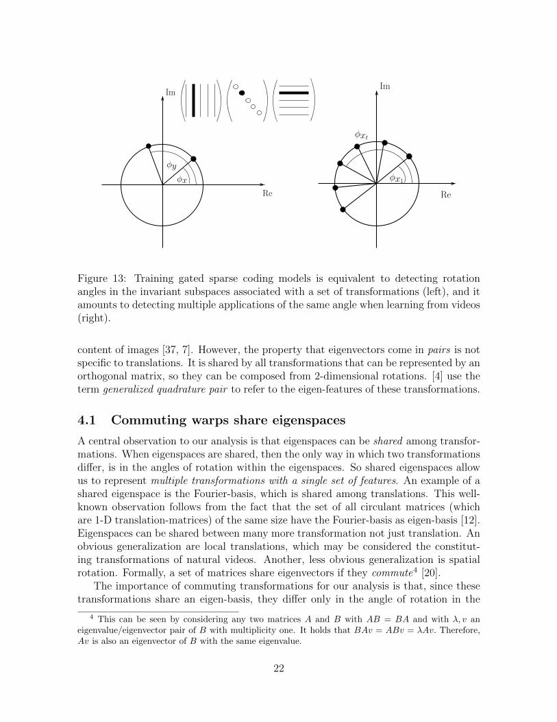
An important fact about orthogonal matrices is that the eigen-decomposition L =UDUT is complex, where eigenvalues (diagonal of D) have absolute value 1 [20]. Multi-plying by a complex number with absolute value 1 amounts to performing a rotation inthe complex plane, as illustrated in Figure 13 (left). Each eigenspace associated with Lis also referred to as invariant subspace of L (as application of L will keep eigenvectorswithin the subspace).

Applying an orthogonal warp is thus equivalent to (i) projecting the image ontofilter pairs (the real and imaginary parts of each eigenvector), (ii) performing a ro-tation within each invariant subspace, and (iii) projecting back into the image-space.In other words, we can decompose an orthogonal transformation into a set of inde-pendent, 2-dimensional rotations. The most well-known examples are translations: A1D-translation matrix contains ones along one of its secondary diagonals, and it is zeroelsewhere3. The eigenvectors of this matrix are Fourier-components [12], and the rota-tion in each invariant subspace amounts to a phase-shift of the corresponding Fourier-feature. This leaves the norm of the projections onto the Fourier-components (thepower spectrum of the signal) constant, which is a well known property of translation.

It is interesting to note that the imaginary and real parts of the eigenvectors of atranslation matrix correspond to sine and cosine features, respectively, reflecting the factthat Fourier components naturally come in pairs. These are commonly referred to asquadrature pairs in the literature. In the special case of Gabor features, the importanceof quadrature pairs is that they allow us to detect translations independently of the local

3To be exactly orthogonal it has to contain an additional one in another place, so that it performsa rotation with wrap-around.

21

φy

φx

Im

Re

Im

φxt

φx1

Re

Figure 13: Training gated sparse coding models is equivalent to detecting rotationangles in the invariant subspaces associated with a set of transformations (left), and itamounts to detecting multiple applications of the same angle when learning from videos(right).

content of images [37, 7]. However, the property that eigenvectors come in pairs is notspecific to translations. It is shared by all transformations that can be represented by anorthogonal matrix, so they can be composed from 2-dimensional rotations. [4] use theterm generalized quadrature pair to refer to the eigen-features of these transformations.

4.1 Commuting warps share eigenspaces

A central observation to our analysis is that eigenspaces can be shared among transfor-mations. When eigenspaces are shared, then the only way in which two transformationsdiffer, is in the angles of rotation within the eigenspaces. So shared eigenspaces allowus to represent multiple transformations with a single set of features. An example of ashared eigenspace is the Fourier-basis, which is shared among translations. This well-known observation follows from the fact that the set of all circulant matrices (whichare 1-D translation-matrices) of the same size have the Fourier-basis as eigen-basis [12].Eigenspaces can be shared between many more transformation not just translation. Anobvious generalization are local translations, which may be considered the constitut-ing transformations of natural videos. Another, less obvious generalization is spatialrotation. Formally, a set of matrices share eigenvectors if they commute4 [20].

The importance of commuting transformations for our analysis is that, since thesetransformations share an eigen-basis, they differ only in the angle of rotation in the

4 This can be seen by considering any two matrices A and B with AB = BA and with λ, v aneigenvalue/eigenvector pair of B with multiplicity one. It holds that BAv = ABv = λAv. Therefore,Av is also an eigenvector of B with the same eigenvalue.

22

joint eigenspace. As a result, one may extract a particular transformation from a givenimage pair (x,y) by recovering the angles of rotation between the projections of x andy onto the eigenspaces. For this end, consider the real and complex parts vR and vI ofsome eigen-feature v. That is, v = vR + ivI, where i =

√−1. The real and imaginary

coordinates of the projection of x onto the invariant subspace associated with v aregiven by vT

Rx and vTI x, respectively. For the output image, they are vT

Ry and vTI y.

Let φx and φy denote the angles of the projections of x and y with the real axis inthe complex plane. If we normalize the projections to have unit norm, then the cosineof the angle between the projections, φy − φx, may be written

cos(φy − φx) = cosφy cosφx + sinφy sinφx

by trigonometric identity. This is equivalent to computing the inner product betweentwo normalized projections (cf. Figure 13 (left)). In other words, to estimate the (cosineof) the angle of rotation between the projections of x and y, we need to sum over theproduct of two filter responses.

Note, however, that normalizing each projection to 1 amounts to dividing by thesum of squared filter responses, an operation that is highly unstable if a projection isclose to zero. Unfortunately, this will be the case, whenever one of the images is almostorthogonal to the invariant subspace. This, in turn, means that the rotation anglecannot be recovered from the given image, because the image is too close to the axis ofrotation. One may view this as a subspace-generalization of the well-known apertureproblem beyond translation, to the set of orthogonal transformations. Normalizationwould ignore this problem and provide the illusion of a recovered angle even when theaperture problem makes the detection of the transformation component impossible. Inthe next section we discuss how one may overcome this problem by rephrasing theproblem as a detection task.

4.2 Detecting subspace rotations

For each eigenvector, v, and rotation angle, θ, define the complex output image filter

vθ = exp(iθ)v

which represents a projection and simultaneous rotation by θ. This allows us to definea subspace rotation-detector with preferred angle θ as follows:

rθ = (vTRy)(vθR

Tx) + (vT

I y)(vθITx) (20)

where subscripts R and I denote the real and imaginary part of the filters like before.Like before, if projections are normalized to length 1, we have

rθ = cosφy cos(φx − θ) + sinφy sin(φx − θ) = cos(φy − φx − θ),

which is maximal whenever φy − φx = θ, thus when the observed angle of rotation,φy−φx, is equal to the preferred angle of rotation, θ. However, like before, normalizing

23

projections is not a good idea because of the subspace aperture problem. We nowshow that mapping units are well-suited to detecting subspace rotations, if a numberof conditions are met.

4.3 Mapping units as rotation detectors

If features and data are contrast normalized, then the projections will depend only onhow well the image pair represents a given subspace rotation. The value rθ, in turn,will depend (a) on the transformation (via the subspace angle) and (b) on the contentof the images (via the angle between each image and the invariant subspace). Thus,the output of the detector factors in both, the presence of a transformation and ourability to discern it.

The fact that rθ depends on image content makes it a suboptimal representationof transformation. However, note that rθ is a “conservative” detector, that takes ona large value only if an input image pair (x,y) is compatible with its transformation.We can therefore define a content-independent representation by pooling over multipledetectors rθ that represent the same transformation but respond to different images.Note that computing rθ involves summing over the two subspace dimensions, which isalso a form of pooling (within subspaces). Thus, encoding subspace rotations requirestwo types of pooling.

If we stack imaginary and real eigenvector pairs for the input and output images,v and vθ, in matrices U and V , respectively, we may define the representation t of atransformation, given two images x and y, as

t = WTP(UTx

)·(V Ty

)(21)

where P is a band-diagonal “within-subspace” pooling matrix, and W is an appropriate“across-subspace” pooling matrix. Furthermore, the following conditions need to bemet: (1) Images x and y are contrast-normalized, (2) For each row uf of U there existsθ such that the corresponding row vf of V takes the form vf = exp(iθ)uf . In otherwords, filter pairs are related through rotations only.

Eq. 21 takes exactly the same form as inference in a gated sparse coding model(cf., Eq. 17), if we absorb the within-subspace pooling matrix P into W . Learningamounts to identifying both the subspaces and the pooling matrix, so training a multi-view feature learning model can be thought of as performing multiple simultaneousdiagonalizations of a set of transformations. When a data-set contains more thanone transformation class, learning involves partitioning the set of orthogonal warpsinto commutative subsets and simultaneously diagonalizing each subset. Note that, inpractice, complex filters can be represented by learning two-dimensional subspaces inthe form of filter pairs. It is uncommon, albeit possible, to learn actually complex-valued features in practice.

Diagonalizing a single transformation, L, would amount to performing a kind ofcanonical correlations analysis (CCA), so learning a multi-view feature learning modelmay be thought of as performing multiple canonical correlation analyzes with tied

24

features. Similarly, modeling within-image structure by setting x = y [38] wouldamount to learning a PCA mixture with tied weights. In the same way that neuralnetworks can be used to implement CCA and PCA up to a linear transformation, theresult of training a multi-view feature learning model is a simultaneous diagonalizationonly up to a linear transformation.

It is interesting to note that condition (2) above implies that filters are normalizedto have the same length. Imposing a norm constraint has been a common approach tostabilizing learning (eg., [38, 29, 43]). It is also common to apply a sigmoid non-linearityafter computing mapping unit activities, so that the output of a hidden variable can beinterpreted as a probability. Pooling over multiple subspaces may, in addition to pro-viding content-independent representations, also help deal with edge effects and noise,as well as with the fact that learned transformations may not be exactly orthogonal.

5 Relation to energy models

By concatenating images x and y, as well as filters v and vθ, we may approximate thesubspace rotation detector (Eq. 20) also with the response of an energy detector:

rθ =((vR

Ty) + (vθRTx))2

+((vI

Ty) + (vθITx))2

= 2((vR

Ty)(vθRTx) + (vI

Ty)(vθITx))

+ (vRTy)2 + (vθR

Tx)2 + (vI

Ty)2 + (vθITx)2

(22)

Eq. 22 is equivalent to Eq. 20 up to the four quadratic terms. The four quadraticterms are equal to the sum of the squared norms of the projections of x and y onto theinvariant subspace. Thus, like the norm of the projections, they contribute informa-tion about the discernibility of transformations. This makes the energy response moreconservative than the cross-correlation response (Eq. 20). However, the peak responseis still attained only when both images reside within the detector’s invariant subspaceand when their projections are rotated by the detectors preferred angle θ.

By pooling over multiple rotation detectors, rθ, we obtain the equivalent of an energyresponse (Eq. 18). This shows that energy models applied to the concatenation of twoimages are well-suited to modeling transformations, too.

5.1 More than two images

Both energy models and cross-correlation models can be applied to more than twoimages. For gated sparse coding, Eq. 20 can be modified to contain all cross-terms, orall the ones that are deemed relevant (for example, adjacent frames in a “Markov”-typegating model of a video). Alternatively, for the energy mechanism, one can computethe square of the concatenation of more than two images in place of Eq. 22.

25

5.1.1 Example: Implementing an energy model via cross-correlation

The close relation between energy models and gated sparse coding makes it possible toimplement one via the other. Figure 14 shows example filters from an energy modeltrained on concatenated frames from videos showing moving random dots5. We traineda gated auto-encoder with F = 256 factors and K = 128 mapping units, where x = yis given by the concatenation of 10 frames. Filters are constrained, such that wxif =wyif . Each 10-frame input shows random dots moving at a constant speed. Speed anddirection vary across movies.

Since the gated auto-encoder, a cross-correlation model, multiplies two sets of filterresponses which are the same, it effectively computes a square, and thus implements anenergy model. In the absence of any within-image structure, all filters learn to representonly across-image correlations. Thus, as predicted by Eq. 19 the energy model, in turn,implements a cross-correlation model.

Figure 14 depicts, separately, the 10 sets of 256 filters corresponding to the 10time-frames. It shows that the model learns spatio-temporal Fourier features which areselective for speed, frequency and orientation.

6 Discussion

Given the predominance of correspondence tasks in vision, it seems conceivable that themain utility of energy models and complex cells is that they can encode relationshipsnot (monocular) invariances.

This suggests that squaring non-linearities, for example, as the transfer function ina feed-forward network, may be useful, in general, in tasks where relations play a role,such as in recognition tasks that involve motion and stereo. In the long term, comput-ing squares and/or cross-products could help reduce the requirement for large, hand-engineered pipelines, which are currently used for solving correspondence problems intasks like depth inference. These typically involve keypoint extraction, descriptor ex-traction, matching and outlier-removal [14]. A learning based system using complexcells may be able to replace parts of the pipeline with a single, homogeneous modelthat is trained from data. This may also help explain how visual cortex may performa large variety of tasks using a single, homogeneous module, which can be trained by asingle type of learning mechanism.

Interestingly, invariant object recognition itself can be viewed as a correspondenceproblem, where the goal is to match an input observation to invariant templates inmemory. [32] discuss a variation of a gated sparse coding model, which may be con-sidered as an approach to invariant recognition through modeling mappings that takeimages to class labels. The input of the model is an image, the output is an orthogo-nal encoding of a class label, and prediction amounts to marginalizing over the set of

5The data and an animation of the learned spatio-temporal features is available at http://

learning.cs.toronto.edu/~rfm/relational

26

Frame: 1 2 3 4

5 6 7 8

9 10

Figure 14: Implementing a cross-correlation model via an energy model via a cross-correlation model. Sequence of filters learned from the concatenation of 10 frames ofmoving random dots.

27

possible mappings. The graphical model is also equivalent to a set of class-conditionalmanifolds or probability distributions, but inference is feed-forward. The model ef-fectively transforms an input into a canonical pose, so that it can be matched witha template, which itself represents the object in some canonical pose. This can helpexplain the similarity, in general, between filters that allow for invariant recognitionand those that allow for selective recognition of transformations. [32] show how “swirlyfeatures” similar to the rotation features in Figures 10 and 11 emerge when learning toperform rotationally invariant recognition. [3] showed that similar features can emergein feed-forward recognition models that contain squaring non-linearities.

Most common object recognition systems are somewhat unrealistic in that theyare trained to recognize single, static views of objects. Real biological systems getto see “movies” of objects that constantly move around or change their relative pose.It is interesting to note that a model that computes squares or cross-products couldautomatically learn to associate object identity with 3-D structure or with articulatedmotion, simply by being trained on multiple, concatenated frames.

Using multiplicative interactions can also be related to analogy making [31]. It canbe argued that analogy making is at the heart of many cognitive phenomena [19]. Aninteresting question is, to what degree an analogy-making module could be a usefulbuilding block in models of higher-level cognitive capabilities. Since gated sparse cod-ing and energy models can be trained with standard, even Hebbian-like, learning (cf.,Section 2.2), analogy-making does not require any uncommon or unusual machinerybesides multiplicative interactions.

Squaring can be approximated using other non-linearities (see, for example, [51]for a discussion). A possible research question is, what type of approximations ofcomputing squares or cross-products may be advantageous computationally and/ormore plausible biologically. Of course, squares could be simulated using a layer of afeed-forward network with sigmoid activations [9]. However, the abundance of matchingand correspondence tasks in vision may provide some inductive bias in favor of genuinemultiplicative interactions or squares.

Another research question is to what degree deviating from exactly commutingtransformations and exactly orthogonal matrices hampers our ability to learn some-thing useful. Existing experiments (for example in [30, 31]) suggest that there is somerobustness, but there has been no quantitative analysis. It is conceivable, that one couldpre-process data-points, such that they can be related through orthogonal matrices, inorder to make them amenable to an energy or cross-correlation model. Interestingly, itseems that one way to do this, would be by transforming data to be high-dimensionaland sparse.

References

[1] E.H. Adelson and J.R. Bergen. Spatiotemporal energy models for the perceptionof motion. J. Opt. Soc. Am. A, 2(2):284–299, 1985.

28

[2] P.A. Arndt, H.A. Mallot, and H.H. Bulthoff. Human stereovision without localizedimage features. Biological cybernetics, 72(4):279–293, 1995.

[3] James Bergstra, Yoshua Bengio, and Jerome Louradour. Suitability of V1 energymodels for object classification. Neural Computation, pages 1–17, 2010.

[4] M Bethge, S Gerwinn, and JH Macke. Unsupervised learning of a steerable basisfor invariant image representations. In B. E. Rogowitz, editor, Human Vision andElectronic Imaging XII, pages 1–12, Bellingham, WA, USA, February 2007. SPIE.

[5] Adam Coates, Honglak Lee, and A. Y. Ng. An analysis of single-layer networks inunsupervised feature learning.

[6] Aaron Courville, James Bergstra, and Yoshua Bengio. A spike and slab restrictedboltzmann machine. In Artificial Intelligence and Statistics, 2011.

[7] D. Fleet, H. Wagner, and D. Heeger. Neural encoding of binocular disparity:Energy models, position shifts and phase shifts. Vision Research, 36(12):1839–1857, June 1996.

[8] B. N. Flury. Common principal components in k groups. Journal of the AmericanStatistical Association, 79(388):892–898, 1984.

[9] K. Funahashi. On the approximate realization of continuous mappings by neuralnetworks. Neural Netw., 2:183–192, May 1989.

[10] J. L. Gallant, J. Braun, and D. C. Van Essen. Selectivity for polar, hyperbolic,and cartesian gratings in macaque visual cortex. Science, 259:1001–4, 1993.

[11] C. Lee Giles and Tom Maxwell. Learning, invariance, and generalization in high-order neural networks. Appl. Opt., 26(23):4972–4978, December 1987.

[12] Robert M. Gray. Toeplitz and circulant matrices: a review. Commun. Inf. Theory,2:155–239, August 2005.

[13] David Grimes and Rajesh Rao. Bilinear sparse coding for invariant vision. NeuralComputation, 17(1):47–73, 2005.

[14] R. I. Hartley and A. Zisserman. Multiple View Geometry in Computer Vision.Cambridge University Press, ISBN: 0521540518, second edition, 2004.

[15] Fritz Heider and Marianne Simmel. An Experimental Study of Apparent Behavior.The American Journal of Psychology, 57(2):243–259, 1944.

[16] Geoffrey E. Hinton. Training products of experts by minimizing contrastive diver-gence. Neural Computation, 14(8):1771–1800, 2002.

29

[17] Geoffrey E. Hinton, Simon Osindero, and Yee-Whye Teh. A fast learning algorithmfor deep belief nets. Neural Comput., 18:1527–1554, July 2006.

[18] Geoffrey F. Hinton. A parallel computation that assigns canonical object-basedframes of reference. In Proceedings of the 7th international joint conference onArtificial intelligence - Volume 2, pages 683–685, San Francisco, CA, USA, 1981.

[19] Douglas R. Hofstadter. The copycat project: An experiment in nondeterminismand creative analogies. Massachusetts Institute of Technology, 755, 1984.

[20] Roger A. Horn and Charles R. Johnson. Matrix Analysis. Cambridge UniversityPress, 1990.

[21] Patrik Hoyer and Aapo Hyvarinen. A multi-layer sparse coding network learnscontour coding from natural images. Vision Research, 42:1593–1605, 2002.

[22] A. Hyvarinen, J. Hurri, , and Patrik O. Hoyer. Natural Image Statistics: A Prob-abilistic Approach to Early Computational Vision. Springer Verlag, 2009.

[23] Aapo Hyvarinen and Patrik Hoyer. Emergence of phase- and shift-invariant fea-tures by decomposition of natural images into independent feature subspaces. Neu-ral Comput., 12:1705–1720, July 2000.

[24] Aapo Hyvrinen, Patrik O. Hoyer, and Mika Inki. Topographic ica as a model ofnatural image statistics. In Seong-Whan Lee, Heinrich H. Blthoff, and TomasoPoggio, editors, Biologically Motivated Computer Vision, volume 1811 of LectureNotes in Computer Science, pages 535–544. Springer, 2000.

[25] Y. Karklin and M. S. Lewicki. Is early vision optimized for extracting higher-orderdependencies? In Advances in Neural Information Processing Systems 18. MITPress, 2006.

[26] Teuvo Kohonen. The Adaptive-Subspace SOM (ASSOM) and its use for the im-plementation of invariant feature detection. In Proc. ICANN’95, Int. Conf. onArtificial Neural Networks, volume I, pages 3–10. EC2, 1995.

[27] Q.V. Le, W.Y. Zou, S.Y. Yeung, and A.Y. Ng. Learning hierarchical spatio-temporal features for action recognition with independent subspace analysis. InProc. CVPR, 2011. IEEE, 2011.

[28] Roland Memisevic. Non-linear latent factor models for revealing structure in high-dimensional data. dissertation, University of Toronto, 2008.

[29] Roland Memisevic. Gradient-based learning of higher-order image features. InProceedings of the International Conference on Computer Vision (ICCV), 2011.

30

[30] Roland Memisevic and Geoffrey Hinton. Unsupervised learning of image trans-formations. In Proceedings of IEEE Conference on Computer Vision and PatternRecognition, 2007.

[31] Roland Memisevic and Geoffrey E Hinton. Learning to represent spatial trans-formations with factored higher-order Boltzmann machines. Neural Computation,22(6):1473–92, 2010.

[32] Roland Memisevic, Christopher Zach, Geoffrey Hinton, and Marc Pollefeys. Gatedsoftmax classification. In Advances in Neural Information Processing Systems 22.MIT Press, 2010.

[33] Izumi Ohzawa, Gregory C. Deangelis, and Ralph D. Freeman. Stereoscopic DepthDiscrimination in the Visual Cortex: Neurons Ideally Suited as Disparity Detec-tors. Science (New York, N.Y.), 249(4972):1037–1041, August 1990.

[34] B. Olshausen and D. Field. Emergence of simple-cell receptive field properties bylearning a sparse code for natural images. Nature, 381(6583):607–609, June 1996.

[35] Bruno Olshausen. Neural Routing Circuits for Forming Invariant Representationsof Visual Objects. PhD thesis, Computation and Neural Systems, 1994.

[36] Bruno Olshausen, Charles Cadieu, Jack Culpepper, and David Warland. Bilinearmodels of natural images. In SPIE Proceedings: Human Vision Electronic ImagingXII, San Jose, 2007.

[37] Ning Qian. Computing stereo disparity and motion with known binocular cellproperties. Neural Comput., 6:390–404, May 1994.

[38] Marc’Aurelio Ranzato and Geoffrey E. Hinton. Modeling Pixel Means and Covari-ances Using Factorized Third-Order Boltzmann Machines. In Computer Visionand Pattern Recognition, pages 2551–2558, 2010.

[39] Marc’Aurelio Ranzato, Alex Krizhevsky, and Geoffrey E. Hinton. Factored 3-WayRestricted Boltzmann Machines For Modeling Natural Images. In Proc. ThirteenthInternational Conference on Artificial Intelligence and Statistics (AISTATS), 2010.

[40] D. E. Rumelhart, G. E. Hinton, and J. L. Mcclelland. A general framework forparallel distributed processing. In Parallel distributed processing: explorations inthe microstructure of cognition, volume 1, chapter 2, pages 45–76. MIT Press, 1986.

[41] T. Sanger. Stereo disparity computation using Gabor filters. Biological Cybernetics,59:405–418, 1988. 10.1007/BF00336114.

[42] Paul Smolensky. Tensor product variable binding and the representation of sym-bolic structures in connectionist systems. Artificial Intelligence, 46:159–216, 1990.

31

[43] J. Susskind, R. Memisevic, G. Hinton, and M. Pollefeys. Modeling the joint den-sity of two images under a variety of transformations. In Proceedings of IEEEConference on Computer Vision and Pattern Recognition, 2011.

[44] Graham, W. Taylor, Rob Fergus, Yann LeCun, and Christoph Bregler. Convo-lutional learning of spatio-temporal features. In Proc. European Conference onComputer Vision (ECCV’10), 2010.

[45] Joshua Tenenbaum and William Freeman. Separating style and content with bi-linear models. Neural Computation, 12(6):1247–1283, 2000.

[46] N Troje and HH Bulthoff. Face recognition under varying poses: The role oftexture and shape. Vision Research, 36(12):1761–1771, 6 1996.

[47] Pascal Vincent, Hugo Larochelle, Yoshua Bengio, and Pierre-Antoine Manzagol.Extracting and composing robust features with denoising autoencoders. ICML ’08,New York, NY, USA, 2008. ACM.

[48] Christoph von der Malsburg. The correlation theory of brain function. Internal re-port, 81-2, Max-Planck-Institut fur Biophysikalische Chemie, Postfach 2841, 3400Gottingen, FRG, 1981. Reprinted in E. Domany, J. L. van Hemmen, and K. Schul-ten, editors, Models of Neural Networks II, chapter 2, pages 95–119. Springer-Verlag, Berlin, 1994.

[49] M. J. Wainwright and E. P. Simoncelli. Scale Mixtures of Gaussians and the Statis-tics of Natural Images. In Adv. Neural Information Processing Systems (NIPS*99),volume 12, pages 855–861, Cambridge, MA, 2000. MIT Press.

[50] Max Welling, Geoffrey E. Hinton, and Simon Osindero. Learning Sparse Topo-graphic Representations with Products of Student-t Distributions. In NIPS 2002,2002.

[51] Christoph Zetzsche and Ulrich Nuding. Nonlinear and higher-order approaches tothe encoding of natural scenes. Network (Bristol, England), 16(2-3):191–221, 2005.

32