Learning to Beat the Random Walk

Using Machine Learning to Predict Changes in Exchange Rates

A Senior Thesis

Presented to

The Faculty of the Economics Department of

Bates College

In partial fulfillment of the requirements for the

Degree of Bachelor of Arts

by

Abdul Tawab Ajmal Safi

Lewiston, Maine

December 6, 2019

Advisor: Julieta Yung,Ph.D.

1

Abstract

In my thesis, I use di↵erent machine learning techniques to predict the directional changein exchange rates. I start o↵ by analyzing Uncovered Interest Rate Parity (UIP) and its failureto predict changes in exchange rates. Using linear regression, I show that the � coe�cient inUIP equation is not equal to zero over the short and long run. This shows the importance ofcurrency risk premium for understanding changes in exchange rates. However, risk premiumand market expectations are extremely di�cult to measure. For this reason, Random Walk isthe best model for predicting changes in the foreign exchange rates over the short run. Thislead me to ask: Can we use the latest machine learning techniques to predict foreignexchange rates more accurately than Random Walk model? I explore various machinelearning techniques including Principal Component Analysis (PCA), Support Vector Machines(SVM), Artificial Neural Networks (ANN), and Sentiment Analysis in an e↵ort to predict thedirectional changes in exchange rates for a list of developed and developing countries.

After exploring relevant literature on exchange rates, I analyze excess returns in the carrytrade market by using historical exchange rate and interest rate data to create a simulationfor trading on a monthly or semi-annual basis. I use the interest rate data of each country tosort them into portfolios for carry trade. The results show that investors can earn large profitsover the short run by borrowing from low interest rate countries’ bond market and investing inthat of high interest rate countries. I also find that the returns on carry trade starts to reduceas the trading interval increases.

According to the spanning hypothesis, the yield curve, its expectation and term premiumcomponent span all relevant information related to the economic performance of a country. Thismeans that the economic situation of a country can be understood by analyzing its bond market.Based on the spanning hypothesis, I use Principal Component Analysis (PCA) to extract thelevel, slope, and curvature of the yield curve and its components. Then, taking the resultantprincipal components, I use Support Vector Machines (SVM) and Artificial Neural Networks(ANN) to predict the directional change in foreign exchange excess returns. Compared to theSVMs, the ANNs more accurately predict the directional change in the exchange rate excessreturns over the short run. This di↵erence is attributed to the ability of Artificial NeuralNetworks to learn abstract features from raw data.

Finally, in the last chapter, I use sentiment analysis to evaluate the tonality of foreignexchange news articles from investing.com to develop a variable for understanding currency riskpremium and market expectations in order to predict the directional changes in the exchangerates. In order to identify the model that most reliably captures the tonality of foreign exchangenews articles, I use five di↵erent sentiment analysis models: Tonality model, VADER model,TextBlob model, Harvard IV-4 Dictionary model, and Loughran and Mcdonald Dictionarymodel. The results show that di↵erent sentiment models better predict the directional changesin exchange rates of di↵erent countries.

Overall, this research finds evidence that machine learning models can more accuratelypredict directional change in exchange rates than the Random Walk model when the inputfeatures used to train the machine learning models are representative of the economic situationof a country. Hence, using macro-economic and financial theory to develop input features thatcapture the most relevant characteristics of a country’s economy can help us understand shortrun movements in the foreign exchange markets.

2

Acknowledgements

I would like to thank Professor Yung for encouraging me to explore and develop di↵erentideas throughout my thesis process. I would also like to thank Francesca for reminding me tosleep, motivating me to keep working hard, and being there for me throughout the semester.Thank you Will, for helping me edit my thesis and giving me advice how to better structuremy sentences. Thank you Aktan, for pulling all nighters with me. Thank you Ghasharib andKush for playing Catan with me to destress. Finally, I would like to thank my parents for alltheir e↵ort and hard work that has allowed me to pursue my dreams.

3

Contents

1 Background 5

2 Testing for UIP 82.1 Regression Analysis . . . . . . . . . . . . . . . . . . . . . . . . . . . . . . . . . . 8

2.1.1 Results . . . . . . . . . . . . . . . . . . . . . . . . . . . . . . . . . . . . . 92.1.2 Discussion . . . . . . . . . . . . . . . . . . . . . . . . . . . . . . . . . . . 12

2.2 Carry Trade Portfolio Simulation . . . . . . . . . . . . . . . . . . . . . . . . . . 122.2.1 Results . . . . . . . . . . . . . . . . . . . . . . . . . . . . . . . . . . . . . 142.2.2 Discussion . . . . . . . . . . . . . . . . . . . . . . . . . . . . . . . . . . . 17

3 Predicting Directional Change in Exchange Rate Returns 183.1 Feature Engineering . . . . . . . . . . . . . . . . . . . . . . . . . . . . . . . . . . 19

3.1.1 Calculating binary variable for directional change in exchange rate returns 203.1.2 Principal components of yield curve and its components . . . . . . . . . . 22

3.2 Support Vector Machine (SVM) . . . . . . . . . . . . . . . . . . . . . . . . . . . 273.3 Artificial Neural Network (ANN) . . . . . . . . . . . . . . . . . . . . . . . . . . 303.4 Discussion . . . . . . . . . . . . . . . . . . . . . . . . . . . . . . . . . . . . . . . 34

4 Sentiment Analysis for Predicting Directional Change in Foreign ExchangeMarket 354.1 Feature Engineering . . . . . . . . . . . . . . . . . . . . . . . . . . . . . . . . . . 364.2 Text Preprocessing . . . . . . . . . . . . . . . . . . . . . . . . . . . . . . . . . . 38

4.2.1 Text cleaning . . . . . . . . . . . . . . . . . . . . . . . . . . . . . . . . . 384.2.2 Text to vector conversion . . . . . . . . . . . . . . . . . . . . . . . . . . . 38

4.3 Sorting Text by Country . . . . . . . . . . . . . . . . . . . . . . . . . . . . . . . 404.3.1 Textual Data Structure . . . . . . . . . . . . . . . . . . . . . . . . . . . . 414.3.2 E↵ectiveness of text sorting algorithm . . . . . . . . . . . . . . . . . . . 42

4.4 Sentiment Analysis . . . . . . . . . . . . . . . . . . . . . . . . . . . . . . . . . . 444.4.1 Methods for Sentiment Analysis . . . . . . . . . . . . . . . . . . . . . . . 444.4.2 Models for Sentiment Analysis . . . . . . . . . . . . . . . . . . . . . . . . 464.4.3 Results . . . . . . . . . . . . . . . . . . . . . . . . . . . . . . . . . . . . . 47

4.5 Discussion . . . . . . . . . . . . . . . . . . . . . . . . . . . . . . . . . . . . . . . 54

5 Conclusion 55

References 57

4

Chapter 1

Background

Exchange rate refers to the value of one currency in terms of another i.e. how much ofone currency can we buy with one unit of another currency. The exchange rate of a countryappreciates when the value of its currency increases in terms of another currency. On theother hand, a currency depreciates when its value decreases in terms of another currency.Globalization has led economics to be more interconnected than ever before, making exchangerates important for both businesses and policy makers. Exchange rates are an important com-ponent of international trade which greatly influences the economic performance of a country.It influences the price of a good in the international market. For example, the exchange rateappreciation of a currency makes a country’s imports cheaper while making exports expen-sive. Higher prices, in terms of other currencies, might make a country less competitive inthe international market leading to a decrease in the demand for its goods. This can havea negative impact on the Gross Domestic Product (GDP) and subsequently the standard ofliving of a country. Hence, it has became increasingly imperative for economists to understandand model exchange rates in order to make wise decisions while conducting international tradeor developing economic policies.

Like other financial variables, changes in exchange rates are very hard to predict over theshort run. This is because they are dictated by changes in the expectations about futureeconomic fundamentals rather than by changes in the current ones. Economic fundamen-tals are macro-economic variables that are hypothesized to explain changes in exchange ratemovements e.g. trade balances, money supply, national income etc. The current value of amacro-variable might vary drastically from its expected value (Wang et al., 2008). This meansthat current economic fundamentals might have very little, if any, use in forecasting exchangerates between countries with almost similar inflation rates. This gives rise to the exchangerate disconnect puzzle, which states that a random walk model does a better job at forecast-ing exchange rates over the short run than a model based on macro-economic fundamentals. Arandom walk model or a naive model is one that predicts the current value of a variable asits future value. It is di�cult to beat the random walk model because exchange rates are morevolatile than any of the candidate macro-economic fundamentals that we have. Another reasonfor the ine�ciency of macro economic fundamentals in forecasting exchange rates is that theirvolatility remains similar across countries, whereas the volatility of exchange rates varies acrossdi↵erent currency pairs. Finally, the exchange rate disconnect puzzle exists because currencyvolatility changes across fixed and floating regimes while the volatility of fundamentals doesnot (Meese & Rogo↵, 1983).

Trading on the foreign exchange market gave rise to the theory of interest rate parity,which states that return on investment in domestic bond market and foreign bond marketshould be the same. This assumes perfect competition and no arbitrage opportunity as pos-

5

itive returns on interest rate di↵erential between countries is cancelled o↵ by changes in theexchange rate. This leads to the idea of uncovered interest rate parity (UIP), which statesthat domestic interest rate should be equal to foreign interest rate plus expected change in ex-change rates. According to Aggarwal (2013), “If investors are risk-neutral and have rationalexpectations, the future exchange rate should perfectly adjust given the present interest-ratedi↵erential.” This means that the expected change in exchange rate over a certain period isequal to that period’s risk-free interest rate di↵erential between the foreign and domestic bondmarket (Aggarwal et al., 2013). Following is the equation for UIP:

Et[st+1]� st = it � i⇤t

In the equation above, Et[st+1]� st indicates the change in exchange rate from one periodto another. We use it to show domestic interest rate and i⇤t to show foreign interest rate. Thesubscript t indicates the current time period, while the subscript t+1 indicates one periodfuture time period. The equation above can be further simplified into the following equation:

�st+1 = it � i⇤t

In the equation above, �st+1 indicates the change in exchange rate from one period toanother. According to the equation, if the domestic interest rate it is greater than the foreigninterest rate i⇤t then the domestic currency will be expected to depreciate for interest rate parityto hold. However, this theory does not hold in reality.

Exchange rate changes are not compensated by interest rate di↵erentials. “If anything,the opposite holds true empirically - high-interest-rate currencies tend to appreciate whilelow-interest-rate currencies tend to depreciate. As a consequence, carry trades form a portfolioinvestment strategy, violate the uncovered interest parity and give rise to the ’forward premiumpuzzle’” (Menkho↵, Sarno, Schmeling, & Schrimpf, 2011). Carry Trade is the most popularinvestment strategy in the foreign exchange market. According to it, we can earn a profit byborrowing from countries with low interest rate and investing in countries with high interestrate. The success of carry trade indicates the failure of UIP which gives rise to the forwardpremium puzzle or the “Fama Puzzle”. According to it, if the domestic interest rate is greaterthan the foreign interest rate it causes the domestic currency to appreciate instead of depreciate,which is contrary to what theory suggests (Fama, 1984). A theoretically convincing and straightforward solution for this puzzle is the consideration of the time-varying risk premium. RiskPremium or Risk Premia is the compensation that risk averse investors require for holdingassets denominated in foreign currencies. Investors in the foreign exchange market are alwaysexposed to currency risk, which is the risk that the value of foreign currency might changeleading to loss. A positive risk premium shows that the investors view a certain foreign currencyas risky asset, while a negative risk premium shows that the investors view a certain currencyas a safe asset. It is the inclusion of the time varying risk premium component in the UIPequation that might help us explain the Fama Puzzle i.e. the negative correlation between expost depreciation and the interest rate di↵erentials.

�st+1 = it � i⇤t +RPt

In the equation above, the RPt indicates the time varying risk premium of the currencymarket. According to the “New Fama Puzzle”, it is not only the risk premium but also thenot unbiasedness of the expectation of exchange rate changes that causes the failure of UIP.Accounting for risk premia alone does not entirely cause the UIP to be true. Hence it will beimportant to integrate an expectation variable extracted from surveys or news paper analysis

6

into our model in order to be consistent with economic theory (Bussiere, Chinn, Ferrara, &Heipertz, 2018).

7

Chapter 2

Testing for UIP

2.1 Regression Analysis

In this section, I am going to test for uncovered interest rate parity by using a univariate OLSregression model. I am going to use monthly change in US dollars in terms of British Pounds(GBP) as the dependent variable. United States is considered as the domestic country whileUnited Kingdoms is considered as the foreign country in the model. The dataset consists ofmonthly data from 1999 to 2019. The model used to test for UIP is adopted from (Hansen &Hodrick, 1980).

�st+n = ↵ + �(it � i⇤t ) + et+n

In the equation above, �st+n indicates the change in exchange rate n periods ahead. ↵ is thevalue of the constant or intercept in the model. et+n shows the time varying error term of themodel. All the residuals of the model are stored in the error term. it� i⇤t indicates the interestrate di↵erential between the domestic and foreign country i.e. US and UK respectively. � showsthe regression coe�cient of the interest rate di↵erential. It indicates how much GBP/USD willmove based on one unit change in the interest rate di↵erential. In order for UIP to hold, ↵should be equal to zero and � should be equal to 1. A � value of positive one indicates thatthe interest rate di↵erential is positively correlated with change in exchange rate. An ↵ valueof zero indicates that there is no constant in the model i.e. all movements in the exchange rateare explained by changes in the interest rate di↵erential.

One might hypothesize that changes in the interest rate di↵erential might take time toinfluence changes in exchange rates. This means that the UIP might not hold over the shortrun but it might hold over the long run. In order to test for this hypothesis, I developed threedi↵erent regression models at varying lagged intervals. The first model checks for the existenceof UIP over the very short run as it regresses changes in current exchange rate on currentinterest rate di↵erential. The second model checks for UIP over a 6 month period by checkingthe e�ciency of the current interest rate di↵erential in predicting changes in the 6 monthahead exchange rate. Lastly, the final model check for UIP over the long run, by checking thee�ciency of current interest rate di↵erential in predicting changes in one year ahead exchangerates. According to theory, UIP does not hold over the short or long run. The � coe�cientover the short run will be less than 0 indicating the existence of risk premium, while it mightbecome positive over the long run (but it never equals 1).

8

2.1.1 Results

UIP Test over Zero Lagged Interval

Dep. Variable: GBP/USD R-squared: 0.051Model: OLS Adj. R-squared: 0.048Method: Least Squares F-statistic: 13.19Date: Fri, 29 Nov 2019 Prob (F-statistic): 0.000343Time: 19:13:35 Log-Likelihood: 603.14No. Observations: 245 AIC: -1202.Df Residuals: 243 BIC: -1195.Df Model: 1

coef std err t P>|t| [0.025 0.975]

Intercept 0.0020 0.001 1.491 0.137 -0.001 0.005x -0.0040 0.001 -3.632 0.000 -0.006 -0.002

Omnibus: 19.218 Durbin-Watson: 1.598Prob(Omnibus): 0.000 Jarque-Bera (JB): 31.069Skew: 0.474 Prob(JB): 1.79e-07Kurtosis: 4.465 Cond. No. 1.32

Figure 2.1: Current change in exchange rate against current interest rate di↵erential

According to the regression results and figure above, the UIP does not hold over the zerolagged interval. The � coe�cient for the interest rate di↵erential has a value of -0.0040 whichis as per the Fama puzzle and it validates the presence of the risk premium component. The �coe�cient is statistically significant at 99% significance level. The intercept ↵ is also not equalto zero. The scatterplot above shows that the interest rate di↵erential is negatively correlatedwith the change in exchange rate which violates UIP. The results indicate that UIP does nothold over the very short run.

9

UIP Test over 6 Month Lagged Interval

Dep. Variable: GBP/USD R-squared: 0.026Model: OLS Adj. R-squared: 0.022Method: Least Squares F-statistic: 6.442Date: Fri, 29 Nov 2019 Prob (F-statistic): 0.0118Time: 19:45:23 Log-Likelihood: 607.42No. Observations: 248 AIC: -1211.Df Residuals: 246 BIC: -1204.Df Model: 1

coef std err t P>|t| [0.025 0.975]

Intercept 0.0018 0.001 1.357 0.176 -0.001 0.005x -0.0028 0.001 -2.538 0.012 -0.005 -0.001

Omnibus: 17.308 Durbin-Watson: 1.545Prob(Omnibus): 0.000 Jarque-Bera (JB): 29.657Skew: 0.403 Prob(JB): 3.63e-07Kurtosis: 4.490 Cond. No. 1.32

Figure 2.2: 6-month-ahead change in exchange rate against current interest rate di↵erential

According to the regression results and figure above, the UIP does not hold over the sixmonth lagged interval. The � coe�cient for the interest rate di↵erential has a value of -0.0028which is as per the Fama puzzle and it validates the presence of the risk premium component.The � coe�cient is statistically significant at 95% significance level. The � coe�cient hasbeen reduced in magnitude and significance compared to the zero lagged regression results.The intercept ↵ is also not equal to zero. The scatterplot above shows that the interest ratedi↵erential is negatively correlated with the change in exchange rate which violates UIP. Theresults indicate that UIP does not hold over the over six month lagged interval.

10

UIP Test over 1 Year Lagged Interval

Dep. Variable: GBP/USD R-squared: 0.003Model: OLS Adj. R-squared: -0.001Method: Least Squares F-statistic: 0.6652Date: Fri, 29 Nov 2019 Prob (F-statistic): 0.416Time: 20:23:40 Log-Likelihood: 604.55No. Observations: 248 AIC: -1205.Df Residuals: 246 BIC: -1198.Df Model: 1

coef std err t P>|t| [0.025 0.975]

Intercept 0.0013 0.001 0.980 0.328 -0.001 0.004x -0.0009 0.001 -0.816 0.416 -0.003 0.001

Omnibus: 25.499 Durbin-Watson: 1.511Prob(Omnibus): 0.000 Jarque-Bera (JB): 49.022Skew: 0.544 Prob(JB): 2.26e-11Kurtosis: 4.887 Cond. No. 1.26

Figure 2.3: 1-year-ahead change in exchange rate against current interest rate di↵erential

According to the regression results and figure above, the UIP does not hold over the one yearlagged interval. The � coe�cient for the interest rate di↵erential has a statistically insignificantvalue of value of -0.0009. This means that there is a possibility that the regression coe�cientis positive instead of negative. This shows that the existence of the Fama puzzle is not certainover the long run i.e. the current risk premium component has little, if any, influence on 1year ahead exchange rate. The intercept ↵ is also not equal to zero. The scatterplot aboveshows that the interest rate di↵erential is still slightly negatively correlated with the change inexchange rate which violates UIP. The results indicate that UIP also does not hold over a 1year lagged interval.

11

2.1.2 Discussion

As the theory suggests, the uncovered interest rate parity (UIP) does not hold over the shortand long run. Our regression results show that the � coe�cient and intercept ↵ at all threelagged intervals were not equal to 1 and 0 respectively. This means that the UIP did not holdtrue at any time interval within 1 year for the GBP/USD currency pair. Over the zero and sixmonth lagged interval, the forward premium puzzle seemed to exist that the � coe�cient wasnegative and statistically significant. This means that the current currency risk premium caninfluence changes in six month ahead exchange rates. This, however, does not appear to bethe case for the one year lagged interval, as the � coe�cient was still negative but statisticallyinsignificant. This indicates that there is a possibility that the � coe�cient might be positive.These results show that the influence of the current currency risk premium on the exchangerate starts to depreciate over time.

2.2 Carry Trade Portfolio Simulation

Carry trade is a popular currency trading strategy that invests in high interest currenciesby borrowing from low interest currencies. “Carry trade is at the core of active currencymanagement and is designed to exploit deviations from uncovered interest rate parity (UIP).If UIP holds, the interest rate di↵erential is an average o↵set by a commensurate depreciationof the investment currency and the expected carry trade return is equal to zero” (Cenedese,Sarno, & Tsiakas, 2014). This means that the popularity of carry trade and the existence ofexcess returns in it indicates the existence of the Fama Puzzle. In order for UIP to hold thereshould be no arbitrage opportunity in the economy which means that carry trade should notbe profitable. This, however, is never the case. In this section, I am going to use basic carrytrade strategy to prove that UIP does not hold.

Carry trade, in the past, has delivered considerable excess returns and a sharpe ratio ofmore than twice that of the US stock market. This has made it into the most popular tradingstrategy in the currency market. However, according to the current literature high profitsin carry trade are no free lunch in the sense that they act as compensation for investors forbearing risk (Cenedese et al., 2014). The returns from carry trade compensate investors forexposure to systematic risk that might lead to large future carry trade losses during periods ofhigh market variance. Interest rate measures the level of the risk in an economy. High interestrates indicate risky currencies that pay the largest premium, while low interest rate currenciesare less risky and o↵er insurance against aggregate risk. The returns for high interest ratecurrencies tend to fall during periods of high economic uncertainty whereas the returns for lowinterest rate currencies tend to rise (Berg & Mark, 2018). It is this behavior of the currencyrisk premium component that explains the forward premium puzzle and the excess returns itcauses in carry trade.

“While the average carry trade is profitable, the performance of the individual carry tradevaries across currencies, with trades against the Swiss Franc earning a low 0.6% annual ex-cess return, and trade against the Danish Krone earning a high 9.3% annual excess return”(Burnside, 2011). Individual currency trading has higher exposure to risk and uncertaintybecause it relies on the economic conditions of only one specific country. According to financialtrading, diversifying an investment portfolio always yields better results than investing in anindividual asset. For this reason, I am going to explore di↵erent weighted carry trade portfoliosusing a diverse set of developed and developing countries. The countries being considered for theanalysis are Australia, Canada, China, Chile, Czech Republic, Colombia, Hungary, Indonesia,

12

Japan, Mexico, Norway, New Zealand, Poland, South Africa, Singapore, Sweden, Switzerland,United Kingdoms, and Brazil. All countries exchange rates are calculated with USD as its basevalue. This is done to calculate the profit a US investor will make by participating in carrytrade.

Excess return in carry trade is the product of the amount of investment with the interestrate di↵erential between the low and high interest rate currencies while accounting for thechange in exchange rates. Transaction cost is another additional expense that needs to beaccounted for while calculating returns on carry trade. In our analysis, for simplicity purposes,I am going to assume our transaction cost to be zero. Percentage return on carry trade variesbased on the trading interval used. Trading on the currency market can be done on daily,weekly, monthly, quarterly, semi-annually, or annual intervals. Craig Burnside (2011)’s carrytrade portfolio strategy earned an average annual profit of 6% with a standard deviation of9.5%. In my analysis, I am going to use monthly and semi-annual trading basis. Using amonthly trading strategy means that during the start of every month currencies are sorted asper their interest rate. Afterwards, a portfolio is constructed shorting the lowest interest ratecurrencies and going long on the highest interest rate currencies. By the end of every monthexcess returns are calculated for the carry trade. A similar procedure with 6 month laggedintervals are used for the semi-annual trading strategy. The formula for calculating the payo↵to carry trade strategy is taken from Craig Burnside (2011):

zt+n = (1 + i⇤t )st+n

st� (1 + it)

In the above equation, zt+n shows the payo↵ for investing one USD in carry trade. i⇤trepresents the interest rate of the country that we are investing in, while it represents theinterest rate of the country we are borrowing from. st+1

strepresents the change in exchange rate

over n period of time.

The dataset used for carry trade analysis consists of monthly treasury bills and exchangerate data ranging from 1999 to 2018. Treasury bills with one month bond maturity are used asa proxy for interest rate of di↵erent countries. Higher bond maturities are not used because theaverage excess return declines to zero as the maturity increases. This means that carry tradestrategy implemented with treasury bills is more profitable than that implemented on longterm bonds (Lustig, Stathopoulos, & Verdelhan, 2013). The carry trade model equips a rollingone month horizon investment strategy. This means that no train or test dataset is requiredfor the development of the model. The model uses basic carry trade strategy, which investsin high interest currencies and borrows from low interest rate currencies, in combination witha weighting mechanism to construct portfolios. Weights are manual assigned by a trader atthe beginning of the trading interval. A weight of “100%” would mean that the model shouldborrow 100% of the investment amount from the country with lowest interest rate and investall of it in the country with the highest interest rate. Similarly, a weight of “60% and 40%”means that the model should borrow 60% from the country with lowest interest rate and 40%from the country with the second lowest interest rate and then invest 60% in the country withthe highest interest rate and 40% in the country with the second highest interest rate. In thenext section, results for di↵erent weights at varying trading intervals are presented.

13

2.2.1 Results

Excess Return of Single Currency Portfolio on Monthly Basis

Figure 2.4: Percentage Profit From Monthly Carry Trade (Weight = [100])

According to the single currency carry trade portfolio strategy, every month 100% the amountof investment is borrowed from the country with the lowest interest rate and invested in thecountry with the highest interest rate. Every month the borrowing and investing countrychanges based on the global changes in interest rate. The average monthly percentage profit fora single currency carry trade portfolio strategy is 10.89%. Single currency trading is extremelyprofitable but volatile and risky at the same time. It can lead to huge profits or huge lossesbased on the economic situation of a country. As we can see the strategy makes its biggest lossaround 2008, which was during the financial crisis. However, the biggest loss of the strategy isabout 10% point smaller than the biggest profit. Diversifying our portfolio by including morecurrencies might be a good idea to minimize loss during times of uncertainty such as the 2008recession.

14

Excess Return of Multi-Currency Portfolio on Monthly Basis

Figure 2.5: Percentage Profit From Monthly Carry Trade (Weight = [40,30,30])

According to the multi-currency carry trade portfolio strategy, every month the investmentamount is borrowed from three countries with the lowest interest rate with 40% , 30% , and30% weight respectively. Afterwards the same weights are used to invest in the top threecountries with the highest interest rate. Every month the borrowing and investing countrieschanges based on the global changes in interest rate. The average monthly percentage profit fora multi-currency carry trade portfolio strategy is 8.29%. Although our average excess returnreduced from the single currency carry trade portfolio, our strategy does not face any majorlosses. Diversifying our portfolio by borrowing from and lending to multiple countries hasreduced our exposure to loss during times of high uncertainty. Our loss during 2008 recessionfrom single currency portfolio strategy to a multi currency portfolio strategy fell from about14% to about 0%. As supported by the theory, diversifying our portfolio leads to a reductionin our average profit and the possibility of loss.

15

Excess Return of Multi-Currency Portfolio on Semi-Annual Basis

Figure 2.6: Percentage Profit From Semi-Annual Carry Trade (Weight = [40,30,30])

According to the multi-currency carry trade portfolio strategy, every half a year the investmentamount is borrowed from three countries with the lowest interest rate with 40% , 30% , and 30%weight respectively. Afterwards, the same weights are used to invest in the top three countrieswith the highest interest rate. Every half a year the borrowing and investing countries changesbased on the global changes in interest rate. The average semi-annual percentage profit for amulti-currency carry trade portfolio strategy is 6.17%. This strategy yields the lowest averageexcess return among all the strategies. The number of losses faced by the trading strategy alsoincreases as the trading interval increases from one month to six months. Longer maturitydate results in higher exposure to risk because of longer time period for a country’s economicconditions to change. This shows that it is more profitable and risk aversive for us to indulgein carry trade over monthly basis rather than semi-annual basis.

16

2.2.2 Discussion

The existence of excess returns in carry trade indicates that uncovered interest rate parity (UIP)does not hold. It shows that exchange rates does not move as per UIP to cancel the e↵ects ofinterest rate di↵erentials which give rise to arbitrage opportunities in the global economy. Ourcarry trade analysis shows that multi-currency portfolio strategy over short trading intervalyields the best profit to loss ratio. As indicated by theory, single currency portfolio strategycan yield bigger profits but it also exposes us to the possibility of making huge losses. Longermaturity multi-currency portfolio strategy yields the worst result among all our carry trademodels. This is because longer maturity horizons leads to greater uncertainty and risk. It alsoshows that UIP might come to hold over the very long term because the profit for carry tradereduces as the trading interval increases. Increasing the trading interval further might lead toa further fall in profit for carry trade till the point where it might become zero. UIP becometrue when the excess return on carry trade becomes zero.

17

Chapter 3

Predicting Directional Change inExchange Rate Returns

The Foreign exchange (FOREX) market is one of the largest financial markets in the world.Transactions worth billions of dollars a day take place in it (Report on global foreign exchangemarket activity, 2013). Predicting accurate directional changes in the forex market is vital forformulating robust monetary policies. The predicted uptrend or downtrend of exchange ratereturns help traders develop e�cient trading and hedging strategies in the foreign exchangemarket. (Galeshchuk & Mukherjee, 2017a)

Exchange rate forecasting methods can be classified into three broad categories: econo-metrics methods, time series models, and machine learning techniques. Econometric methodsbased on fundamental analysis that is used to predict exchange rates have had limited successover the short run horizon i.e. less than a year (Meese & Rogo↵, 1983). “Time series modelsproduce acceptable point estimates in foreign exchange rate prediction tasks, but are poor atpredicting the direction in which the rates move. Machine Learning methods such as shal-low Artificial Neural Networks(ANN) and Support Vector Machines(SVM) may be marginallybetter at predicting the direction of change but their success depends critically on the inputfeatures used to train the models. However this improvement comes at a considerable cost:obtaining a good set of features from raw input data require significant e↵ort from domain ex-perts” (Galeshchuk & Mukherjee, 2017b). The reason why machine learning algorithms such assupport vector machines and artificial neural networks are better able to perform at predictingthe directional change in exchange rates is because of their ability to fit to non-linear datasets.Most of the econometric methods and times series models used are based on the assumptionof linearity. However, this is not always the case, especially in the financial markets. Hence,non-linear models tend to perform better than linear models in predicting changes in financialmarkets. Deep neural networks, with su�cient data and the right set of features for input, caneasily outperform a support vector machine. This is because these algorithms have the abil-ity to learn abstract features from raw data which may provide improved predictive accuracy.Deep learning algorithms can identify various complex relationships between the feature setand the dependent variable which can help improve the accuracy of predicting the directionalchange in exchange rates. These algorithms, however, are very complex to interpret because oftheir nature of operating like a “black box.” Artificial Neural Networks, like all deep learningalgorithms, also do not perform well on small datasets and might end up overfitting to thetraining dataset. Overfitting is when our model is not generalizable beyond the dataset weused to train it and hence does not perform well on the test dataset. Support Vector Machines,on the other hand, works fairly well with smaller datasets and are less likely to overfit than

18

deep neural networks (Thu & Xuan, 2018).

The expression “directional prediction” refers to the fact that our prediction will not bea point estimate or target value, but a simple “buy” or “sell” recommendation. A positiveforeign exchange market excess return indicates a buy, while a negative foreign exchange marketexcess return indicates a sell. Predicting directional change in exchange rates is a task ofbinary classification which can be done with supervised machine learning algorithms such asANNs and SVMs. Supervised machine learning algorithms are models that require a trainingdataset, containing the set of features and their respective labels, as its input before it canmake predictions on the new set of features. The training dataset needs to be diverse enoughto account for all possible scenarios in order to construct a generalizable model.

This chapter is divided into the following sections: Feature Engineering, Support VectorMachine, Artificial Neural Network, and Discussion. In the feature engineering section, I amgoing to develop an equation for calculating exchange rate excess returns, then I will use amachine learning technique called Principal Component Analysis (PCA) to extract the level,slope and curvature of short and long term yields for all countries in the dataset, and finally Iwill create a binary variable for directional change using exchange rate returns. In the supportvector machine section, I am going to use the PCA extracted variables along with binaryvariable for directional change to train a support vector machine and test its e�ciency usinga test dataset. In the artificial neural network section, I am going to use the same trainingdataset as in the case of SVM to train a deep neural network and to use it to make predictionson the test dataset in order to check for its e�ciency. Finally, in the discussion section, I amgoing to wrap o↵ the chapter by highlighting the main takeaways and discussing any furtherwork that can be done to improve performance.

3.1 Feature Engineering

Feature engineering is the process of using domain knowledge to develop new variables andfeature sets that can help improve the performance of a machine learning algorithm. Featureengineering is a fundamental concept in machine learning that di↵erentiates a good model froma bad model. If done correctly, it increases the predictive power of machine learning algorithmsby creating features from raw data that help facilitate the learning process. In this section, Iam going to first create a binary variable for directional change in exchange rate returns whichwill be used as the dependent variable (the variable we are trying to predict) in our machinelearning algorithms. Afterwards, I am going to use principal component analysis (PCA) onshort and long term yield curves to extract its level, slope, curvature components. The principalcomponents of the yield curve will be used as the predictors or independent variables in ourmachine learning algorithms i.e. I am going to test for how e↵ective di↵erent components ofyield curve are in predicting directional change in exchange rate returns.

19

3.1.1 Calculating binary variable for directional change in exchangerate returns

In order to calculate a binary variable for directional change in foreign exchange excess returns,it is first important for us to calculate exchange rate returns for each country in our dataset.The set of countries being considered are Australia, Canada, China, Chile, Czech Republic,Colombia, Hungary, Indonesia, Japan, Mexico, Norway, New Zealand, Poland, South Africa,Singapore, Sweden, Switzerland, United Kingdoms, and Brazil. The complete dataset consistsof monthly data ranging from May 2007 to February 2019. The dataset has been divided intoa training data and a test data. The training data consists of data ranging from May 2007 toAugust 2015, while the test data consists of data ranging from September 2015 to February2019. The training dataset is used to train our model while the test dataset is used to check theout of sample performance of our machine learning algorithm. After doing the train/test split,exchange rate excess returns are calculated with the following formulae derived from (Bekaert& Hodrick, 1992):

rsit+1 = sit+1 � sit

In the equation above, rsit+1 indicates the exchange rate excess return for a country attime t+1. Subscript i indicates the currency being considered. The variable sit+1 indicates theone period ahead exchange rate of a country, while sit indicates the current exchange rate ofa country. A positive exchange rate excess return indicates a profit, while a negative excessreturn indicates a loss. The graph below shows the percentage exchange rate return of allcountries in our dataset:

20

Figure

3.1:

Mon

thly

Exchan

geRateReturn

forallcountries

fortraindataset

(2007-2015)

21

In the figure above, China appears to have the least volatility in exchange rate returns.This is because China is a fixed exchange rate regime that pegs its currency against the USD.It is also interesting to see how almost all currencies faced an instant fall in excess returnsduring the 2008 financial crisis. This is because all currencies have USD as its base value.It seems that during the 2008 recession USD depreciated in terms of most currencies in thedataset leading to a negative return.

After calculating the exchange rate returns for each country, I used the following formulato develop a binary variable for change in foreign exchange excess returns:

dit+1 =

(1 if rsit+1 > 0

0 if rsit+1 <= 0(3.1)

In the equation above, dit+1 indicate the binary variable that shows the directional changein exchange rate return at time t+1. Subscript i shows the currency being considered. Thebinary variable dit+1 is given a value of one if the excess return is positive and it is given a valueof zero if the excess return is less than or equal to zero. A value of one indicates “buy”, while avalue of zero indicates a “sell”. This means that a trader will be recommended to buy a foreignexchange currency when the excess return is positive and sell when the exchange rate returnis negative. I am going to use this binary variable to train a machine learning model that canhelp us make buy/sell decision based of yield curve components of a country. A buy simplyshows a profit in the foreign exchange market while a sell shows loss in the foreign exchangemarket.

3.1.2 Principal components of yield curve and its components

Principal Component Analysis(PCA) is a dimensionality reduction machine learning techniquethat helps us project a multi-dimensional variable onto to a lower dimensional space. Ineconomics, the yield curve is a curve showing several yields or interest rates for governmentbonds across di↵erent maturity length. A normal yield curve slopes upward, reflecting the factthat the long term interest rates are usually higher than the short term interest rate. The longterm interest rate is determined by the expected future path of the short term interest rateplus a time varying bond risk premium or term premia:

ynt =1

n

n�1X

i=0

E[y1t+i] + TP nt

The equation above shows a long term interest rate with n time period ahead maturity.The variable E[y1t+i] shows the expectation of the one month interest rate i period ahead inthe future. TP n

t shows the term premium or bond risk premium. It shows the compensationthat investors require to invest in longer term bonds.

The initial dataset for principal component analysis consists of the yield curve, and itsexpectation and term premium component. The expectation component of the yield curveinforms us about the market expectation of short run yields, while the term premium compo-nent of the yield curve tells us about uncertainty and volatility in the bond market. Accordingto the spanning hypothesis, the yield curve and its components incorporate all the valuableinformation about the economic situation of a country. This means that the information aboutall macro-economic variables of an economy are already incorporated within the yield curve(Salem et al., n.d.). Hence, the yield curve and its components should have predictive powerin forecasting exchange rate returns because of their ability to span di↵erent macro-economicvariables related to a country. Including all maturities for yields, expectation components, and

22

term premium components as individual variables for each country will be computationallyexpensive and will introduce noise into the model. The yield curve and its components sumup to 357 variables for each country. In order to reduce the dimensionality of our featureset, I am going to use PCA on yield curve and its components individually to extract their“level”, “slope”, and “curvature” components. According to economic literature, the first threeprincipal components of the yield curve represent the “level”, “slope”, and “curvature” of allits maturities (Patel, Mohamed, & van Vuuren, 2018). Taking the PCA of the yield curve,expectation and term premium allowed us to extract level, slope and curvature variables foreach of them. The nine new variables extracted accounted for more than 95% of the variancein our initial dataset of 357 variables. This mechanism helped us take into account all valuableinformation regarding all maturity levels while reducing the computation time for our models.The final nine variables that are going to be used to train our machine learning algorithms are:yield level, yield slope, yield curvature, expectation level, expectation slope, expectation cur-vature, term premium level, term premium slope, and term premium curvature. The followinggraphs shows the principal components for yield curve for all countries in the dataset:

23

Figure

3.2:

Yield

Level

forallcountries

fortrainingdataset

(2007-2015)

24

Figure

3.3:

Yield

Slopeforallcountries

fortrainingdataset

(2007-2015)

25

Figure

3.4:

Yield

Curvature

forallcountries

fortrainingdataset

(2007-2015)

26

In the figures above, China appears to be the most stable across all three principal com-ponents of the yield curve. It is also interesting to see how Chile appears relatively normalin yield level but faces drastically increased volatility in the slope and curvature component.Further economic research will be required to understand why principal components of yieldcurves vary across countries. This however is beyond the scope of this thesis.

Similar to the yield curve, principal components for the expectation and term premiumcomponent of the yield curve were also calculated. Afterwards, the derived components for eachcountry were di↵erenced with that of US. This is done to calculate the economic performanceof a country relative to the United States. As USD is used as the base currency for tradingon the foreign exchange market. It will be valuable to look at the economic performance of acountry relative to the US in order to predict the directional change in foreign exchange excessreturns.

3.2 Support Vector Machine (SVM)

In this section, I am going to present the performance of the country specific SVM modelsdeveloped based on our feature engineered training dataset. A support vector machine is amachine learning algorithm that is widely used for classification tasks. It is a discriminativeclassifier formally defined by a separating hyperplane. Given a labelled training dataset, theSVM outputs an optimal hyperplane which categorizes our dataset into buy and sell categoriesbased on the principal components of yield, expectation, and term premium. This hyperplaneis then used to categorize out of sample data by plotting it on the feature space and determiningwhere the new data points lie compared to the hyperplane. The optimal hyperplane have n-1dimensions, where n determines the dimensions of the feature space. The hyperplane will bea line in a two dimensional vector space, a plain in a three dimensional vector space and soon. Support Vector Machines have di↵erent parameters that needs to be adjusted in order toaccurately classify a dataset. A machine learning technique called Grid Search was used toidentify the best parameters for our SVM model. Grid Search is the process of performinghyperparameter tuning in order to identify the best parameters for a given model. It playsan important role in machine learning as the performance of an entire model is based on theparameter values defined. After developing SVM models for predicting directional change inexchange rate return for all currencies in our dataset, I used a confusion matrix to checkthe performance of our models. A confusion matrix is a table that is used to describe theperformance of a classification model. It creates a table that shows the true positives, falsepositives, false negatives, and true negatives of our model. True positive is when the modelpredicts a positive value when the actual value is positive. False positive is when the modelpredicts a positive value when the actual value is negative. False negative is when the modelpredicts a negative value when the actual value is positive. True negative is when the modelpredicts a negative value when the actual value is negative. A good performing model is onein which the number of true positive and true negatives are greater than the number of falsenegatives and false positives. Confusion matrices for both training and test datasets for allcountry SVM models were created in order to check their e�ciency in predicting directionalchange in foreign exchange excess returns:

27

Figure

3.5:

SVM

Con

fusion

Matricesforallcountries

forTrainingDatasets

28

Figure

3.6:

SVM

Con

fusion

Matricesforallcountries

forTestDatasets

29

According to the results above, most SVM models perform better than random walk ontraining datasets. A random walk model is equivalent to taking a random guess which, on anequally distributed dataset, will have an accuracy of 0.5 or 50%. A model with an accuracyof 0.5 is better than a random walk model in predicting directional change in exchange ratereturns. In case of test datasets, most countries act similar to a random walk model i.e.they keep predicting the same value across the time period. Only a small number of modelsperform better or worse than random walk in the test dataset. The di↵erence between theperformance of models on training and test datasets indicate that the models generated arenot very generalizable. This means that most models do not perform well on out of sampledatasets. An artificial neural network might perform better than an SVM classifier because oftheir ability to identify complex patterns and features in raw data.

3.3 Artificial Neural Network (ANN)

In this section, I am going to present the performance of the country specific ANN modeldeveloped based on our feature engineered training dataset. Artificial neural networks aredeep learning algorithms that try to replicate how the human brain is structured. Like in ahuman brain, the basic building block of a neural network is a neuron that receives some inputand fires an output. Similarly, an artificial neural network consists of nodes that take in valuesor text as input, performs some computation on them, and produces a single output value.An ANN consists of multiple hidden layers, which is a collection of nodes or neurons, withconnections between di↵erent hidden layers. These layers transform data by first computingthe weighted some of inputs and then normalizing the result using some kind of activationfunction assigned to the nodes.

Figure 3.7: Structure of an Artificial Neural Network

A artificial neural network consists of an input layer, multiple hidden layers, and an output

30

layer. All ANN has only one input layer and one output layer, however, the number of hiddenlayers between di↵erent algorithms vary based on the complexity of the problem. The inputlayer is where the data is entered into the algorithm, while the output layer is where the resultis generated. In our case, the output layer will either generate a result of 0 or 1 based onwhether the prediction is a buy or sell. Each hidden layer in the neural network can have anactivation function of its own. A neural network with more than two hidden layers is calleda deep neural network. A neural network makes a prediction by learning the weights of eachnode at every layer. The weights for each node are determined by an algorithm called backpropagation. An ANN with two hidden layers was developed for each country in the datasetto predict the directional change in their foreign exchange returns. The first hidden layer ofthe neural network consists of 64 nodes, while the second hidden layer of the neural networkconsists of 32 nodes. A rectifier activation function is used in the hidden layers, while a sigmoidactivation function is used in the output layer. Sigmoid activation function are used in theoutput layer for binary classification as its output values range between 0 and 1. Rectifier orReLu activation function is the most popular activation function used for classification taskswhich outputs x if x is positive and 0 otherwise. One thousand epochs were run for eachmodel to repetitively improve the model using back propagation. Confusion matrices usingboth training and test datasets were created to access the performance of our ANN models inpredicting directional change in exchange rate returns for a specific currency:

31

Figure

3.8:

NeuralNetworkCon

fusion

Matricesforeach

country’sTrainingDataset

32

Figure

3.9:

NeuralNetworkCon

fusion

Matricesforeach

country’sforTestDataset

33

According to the results above, most countries’ ANN models perform better than randomwalk on training dataset. In case of test datasets, unlike our SVM models, most countries’models perform better than the random walk. It appears that our neural network classificationare more generalizable than our SVM classification models. Although our ANN model are alsoequivalent to random walk for many countries, this might be because of our small trainingdataset size. The performance of our ANN models might improve if we use hourly or dailydata instead of monthly datasets.

3.4 Discussion

Artificial neural networks compared to support vector machines do a better job at predictingdirectional change in exchange rate returns over the short run horizon. This is because oftheir ability to learn abstract features from raw data. According to the financial literature,market expectations and uncertainty variables play an important role in determining directionalchanges in exchange rates. Hence, we might we able to improve the accuracy of our deepneural network models and SVM models by adding a sentiment variable extracted from foreignexchange news articles. Using other forms of deep learning algorithms such as convolutionalneural networks or recurrent neural networks might also improve our accuracy in predictingdirectional change in excess returns. Convolutional neural networks are a form of deep neuralnetworks that are mostly used to analyze visual imagery, but recently it has seen a lot ofsuccess in predicting directional change in exchange rates (Galeshchuk & Mukherjee, 2017b).Recurrent Neural Networks (RNN) are deep neural networks that can use their internal state(memory) to process sequences of inputs. RNN uses the previous predicted state as an inputwhile making new predictions which can also potentially improve the accuracy of our models.Finally, it will be useful to use hourly or daily data instead of monthly dataset as machinelearning algorithms tend of perform better with larger datasets.

34

Chapter 4

Sentiment Analysis for PredictingDirectional Change in ForeignExchange Market

Currency exchange is one of the vital components of international trade and macro-economics.The foreign exchange market is the biggest financial market in the world consisting of transac-tions worth billions of dollars a day (Report on global foreign exchange market activity, 2013).Traders that participate in these markets include governments, financial institutions, and re-tail investors.“In an increasingly challenging and competitive market, having an estimate ofcurrency movements is a holy grail” (Jin et al., 2013). Predicting accurate directional changein the forex market is vital for formulating robust monetary policies. The predicted uptrend ordowntrend of the foreign exchange market helps traders develop e�cient trading and hedgingstrategies in the currency market (Galeshchuk & Mukherjee, 2017a).

Understanding human behavior plays a vital role in predicting directional changes in fi-nancial markets over the short run. Traders filter financial news to identify signals for tradingmarkets. Financial markets are quite sensitive to unanticipated news articles and events. Thismeans that we can predict directional change in currency markets by developing models toanalyze financial news articles. However, identifying the e↵ect of news articles on the currencymarket is an extremely challenging task. This is because of the di�culty in identifying theoptimal methodology for transforming our textual data into numeric values. Econometric ormachine learning algorithms can only understand data in numeric format. This makes it nec-essary for us to transform our textual data from text to numeric format which might cause alose of valuable information. “Most existing literature on financial text mining or sentimentanalysis relies on identifying a predefined set of keywords and machine learning techniques.These methods typically assign weights to keywords in proportion to movement of an exchangerate currency” (Schumaker & Chen, 2006). Sentiment analysis is the most common naturallanguage processing methodology used for predicting change in financial markets. NaturalLanguage Processing is an inter-disciplinary field of linguistics, computer science, informationengineering, and artificial intelligence concerned with how to program computers to processand analyze large amounts of textual data. In sentiment analysis, articles with predefined pos-itive sentiment values (as measured by a sentiment dictionary) are related with positive changein the foreign exchange market, whereas articles with negative sentiment values are associatedwith negative change in the foreign exchange market (Calomiris & Mamaysky, 2019). Re-cently, economists have started to use sentiment analysis on twitter data, google searches, andthe news to predict changes in financial markets such as the stock exchange. This is becausemachine learning techniques are based on textual analysis tend to perform much better than

35

linear regression or any other form of econometric models over the short run. (Schumaker &Chen, 2006).

Term premium and expectation components plays a vital role in predicting exchange ratesover the short run horizon. Foreign exchange news articles are a great source for determiningmarket expectation and uncertainty within the currency market. In this chapter, I am goingto use sentiment analysis and natural language processing on financial news articles to pre-dict directional change in exchange rates. Textual analysis with natural language processingis usually divided into the following steps: collecting raw data, cleaning dataset, structuringdataset, and filtering dataset. The collecting raw data stage consists of web scraping or access-ing internal databases to gather textual data for analysis. The cleaning dataset stage consistsof removing irrelevant textual information such as HTML tags and invalid observations. Thestructuring dataset stage consists of adding tags to describe our textual data (name-entitydetection) and application of sentiment analysis to text. Finally, the filtering dataset stagefocuses on identifying the most relevant entries that would describe a directional change in theforeign exchange market.

Similar to the widely used textual analysis methodology discussed above, this chapter hasbeen divided into the following sections: Feature Engineering, Text Preprocessing, Sorting Textby Country, Sentiment Analysis and Discussion. The feature engineering section describes allthe variables used in our analysis and how they were derived. In the text preprocessing section,I am going to discuss the text cleaning techniques used to get rid of irrelevant information inour dataset. Additionally, I am also going to discuss the text to vector conversion techniqueused to project the textual dataset onto a vector space. In the sorting text by country section,I am going to develop an algorithm using machine learning techniques such as Word2Vec andcosine similarity to distribute financial news articles by country. In the sentiment analysissection, I am going to use five di↵erent sentiment analysis techniques to analysis the sentimentin order to predict directional change in the foreign exchange market. Finally, in the discussionsection, I will end the chapter by highlighting main takeaways and discussing any further workthat can be done to improve performance.

4.1 Feature Engineering

Feature engineering is the process of using domain knowledge to develop new variables andfeatures sets that can help improve the performance of machine learning algorithms. Featureengineering is a fundamental concept in machine learning that di↵erentiates a good model froma bad model. If done correctly, it increases the predictive power of machine learning algorithmsby creating features from raw data that help facilitate the learning process. In this section, Iam going to develop variables to calculate change in exchange rates and store text data basedon financial news articles. The set of countries being considered are Australia, Canada, China,Chile, Czech Republic, Colombia, Hungary, Indonesia, Japan, Mexico, Norway, New Zealand,Poland, South Africa, Singapore, Sweden, Switzerland, United Kingdoms, and Brazil. Thecomplete dataset consists of daily data ranging from 2009 to 2019. The first variable generatedis the change in the exchange rate which is represented by the equation below:

�sit =sit � sit�1

sit�1

In the equation above, �sit represents the daily change in the exchange rate for a countryat time t. Subscript i indicates the currency being considered. The variable sit indicates the

36

exchange rate of a country at time t, while the variable sit�1 indicates the exchange rate of acountry one period before time t. All foreign currencies in the dataset has USD as its basevalue. �sit is the dependent variable in our model i.e. it is the variable that we are going totry to predict using sentiment analysis on financial news data.

The financial news articles for our analysis were collected from investing.com using webscraping. Web scraping is technique used for extracting data from a website. The textualdataset consists of all foreign exchange news articles from 2009 to 2019 recored on daily fre-quency. The total dataset consists of about 82,500 news articles. The graph below shows thedaily news release frequency on investing.com from 2009 to 2019:

Figure 4.1: Daily FOREX News Release Frequency on from 2009 to 2019

In the Figure 4.1, the daily news frequency appears to increase significantly from 2009 to2011. This might be a result of an increase in the financial and economic uncertainty causedby the financial crisis in 2008. After around 2012, the number of foreign exchange news articlerelease appear to go down to an average of 20 articles per day. It is expected for the numberof daily news releases to increase during 2016 as a result of Brexit. This, however, does notappear to be the case. This may be a result of a drop in business for investing.com after 2012,which might be a caused by an increase in competition from financial news such as Bloomberg.In the next section, I am going to discuss the text preprocessing techniques used to prepareour news article data for sentiment analysis.

37

4.2 Text Preprocessing

In order to use our news article dataset for sentiment analysis, we will need to clean it andconvert it into vector format. Text cleaning allows us to eliminate any noise that might influ-ence our analysis. Computers can only understand data in numeric format. Hence, after thetext cleaning process, we will need to convert the remaining dataset into vector format usingtechniques such as “bag of words” or TF-IDF vectorization. This process of text cleaning andtext to vector conversion is known as text preprocessing.

4.2.1 Text cleaning

Natural language processing is both a time and memory consuming process. Cleaning textualdata before converting it into vectors reduces run time. It also helps us avoid extra memoryallocation by getting rid of content that might introduce noise in the dataset. This helps usfocus on content that is most relevant to our analysis. Text cleaning takes place in the followingorder:

• Removing the HTML Tags: Our text data contains HTML tags because the datasetwas scraped from investing.com (eg: < p >, < h2 > etc). HTML tags do not provide anyuseful insight during the sentiment analysis process. It is important to get rid of themin order to eliminate noise into the dataset.

• Removing Punctuations: Similar to HTML tags, punctuation adds unnecessary extradetail. Hence it is a good idea to eliminate them in order to save memory space andcomputational time.

• Removing Stop words: Stop words like “this”, “there”, “is”, “make” etc can also beunnecessary. However, it is important to be cautious while getting rid of stop words like“not” because they can be critical to interpreting data.

• Stemming: This is the process of extracting root words from a text. Words like “taste-ful”, “tastefully” etc are all variations of the word “tasty”. Instead of having to create avector for each of these words, it is better to stem all the words to their root as it helpsbetter analyze and interpret the textual dataset.

• Lemmatization: Similar to stemming, lemmatization is used to convert a word back toits base form. However, this process uses a dictionary for vocabulary and morphologicalanalysis of words. While stemming processes words individually, lemmatization alsoconsiders the context in which it is being used. Lemmatization, for example, can identifythat “good” is the base form of ’better’ while stemming will not account for this.

• Converting words to lower case: Words like “Biscuit” and “biscuit” are classifieddi↵erently because computers cannot di↵erentiate between the uppercase and lowercaseform. For this reason, it is important to convert all textual data to lower case form inorder to enhance model performance.

4.2.2 Text to vector conversion

Next, we will need to convert the dataset into numeric or vector form. There are multipletechniques that can be used to project text onto a vector space. The three techniques used inthis paper are:

38

• Bags of Words: This is the simplest method for projecting text onto a vector space.This technique creates a dictionary of “n” words where “n” is the number of uniquewords in our text corpus. It then creates an “n” dimensional vector for each of ourdocuments in the dataset. Each cell (or dimension) in the bag of words has a valuerepresenting the number of times the corresponding word has occurred in the document.As the vocabulary of the whole dataset increases, the number of dimensions in the bag ofwords also increases. This means that for each document in a big dataset the number ofzeros will exceed the number of non-zeros. Vectors which contain a majority of zeros arereferred to as sparse vectors. Many sparse vectors stacked on top of each other create agrouping called a sparse matrix.

• Term Frequency-Inverse Document Frequency (TF-IDF): This is a more ad-vanced text to vector conversion technique that contains two concepts: Term Frequency(TF) and Inverse Document Frequency (IDF). Term Frequency (TF) refers to the fre-quency of a word appearing in a document. TF aims to identify words that occur themost in a document. It can be represented as:

TF =Number of times a word appear in the document

Total number of words in the document

Inverse Document Frequency(IDF), on the other hand, aims to find the importance of aword by checking its uniqueness across the complete dataset. IDF is based on the ideathat words that are less frequent across the documents but frequent within a specificdocument are critical to understanding that specific document.

IDF = log10Total number of documents

Number of documents in which word appears

TF-IDF is a multiplication of the TF and IDF equations. It aims to identify the wordsthat are unique to a specific document in order to better understand the content of atext. Multiplication of TF with IDF helps reduce the values for high frequency commonwords that occur across most of the dataset. It is a powerful technique that can be usedfor classifying text with di↵erent writing styles because it can identify words that areunique to a document.

• Word2Vec: This is the most advanced and time consuming text to vector conversiontechnique among Bags of Words and TF-IDF. Word2Vec consists of all the deep learningmodels that can be used for generating word embedding. A word embedding is anapproach for providing a dense vector representation to a set of words that capturessomething about their meaning. The vector space representation of the words providea projection where words with similar meanings are clustered together. These modelsconsist of a shallow two layer neural network with one input layer, one hidden layer andone output layer. It is through the use of these pre-trained neural networks that wecan generate word embeddings for textual data. The two main architectures utilizedby Word2Vec models are Continuous Bag of Words (CBOW) and Skip Gram. It isthrough the use of these word embedding techniques over other word to vector conversiontechniques that has lead to breakthrough performance with deep neural networks onproblems such as machine translation.

39

4.3 Sorting Text by Country

After preprocessing foreign exchange news articles, I am going to sort them by country in orderto perform currency specific sentiment analysis. The list of countries that are being consideredare Australia, Canada, Chile, China, Colombia, Czech Republic, Hungary, Indonesia, Japan,Mexico, Norway, New Zealand, Poland, South Africa, Singapore, Sweden, Switzerland, UnitedKingdoms and Brazil. The complete textual dataset contains about 82,500 news articles. Itwould be very time consuming (and almost impossible) to manually go through all the articlesand group them by country. For this reason, I developed a sorting mechanism that searchesfor country specific words in a document along with word embedding and cosine similarity toincorporate any document that might have been left out. A combination of straight forwardsearching and cosine similarity based searching is used to optimize sorting e�ciency. Both thetechniques are explained below:

• Search for specific country related terms: This method involves searching throughall the documents in the dataset for country specific search terms. To do this, I firstdeveloped a specific list of search terms for each country with the following format:[country name, currency code, citizenship]. Every country had these three words intheir list of search terms. For example, in case of Australia the search terms were[australia, aud, australian]. After creating a list of search terms, every document inthe dataset was looped over in order to identify country specific news articles. Everydocument was classified into a di↵erent country based on the search terms it contained.Finally, all the results were organized into separate news article data frames for eachcountry.

• Search based on cosine similarity: Simply searching for specific search terms to clas-sify data is not the most e↵ective way to sort textual data by country because their alwaysremains a possibility that we might be missing some country specific search terms thatare important for grouping our news articles. This means that there is always a chanceof leaving out articles that are related to a country. In order to minimize the probabilityof misclassifying valuable news articles, I combine the searching process with a text simi-larity technique called cosine similarity. Text similarity is the process of determining how“close” two pieces of text are, both in lexical (surface closeness) and semantic (mean-ing) similarity. These techniques make use of word embedding to represent documentsin multi-dimensional vector space and compare documents by measuring the distancebetween the vectors in the feature space. Cosine similarity is one of the most widely usedmethods for text similarity. It calculates the similarity between texts by measuring thecosine of the angle between two vectors. The cosine similarity index ranges from 0 to 1where 0 indicates the least similar, while 1 indicates perfect similarity. It is beneficial touse this technique while sorting data by country because it enables us to account for anycountry specific terms that might have been missed. For example words like “Toronto”and “Ontario” have more than 0.5 cosine similarity with “Canada”. This means we cansimply use a country name along with cosine similarity to search for all articles relatingto it. In order to apply the technique based on cosine similarity, each document in thedataset was projected on a vector space using Word2Vec. Afterwards, the same coun-try specific search terms used in previous searching methods were also projected onto avector space. Finally, any document containing text that had a cosine similarity of morethan 0.5 with a specific country’s search term was classified accordingly. All results wereorganized into country specific dataframes.

• Combining both search results: Once individual news article dataframes for eachcountry were created, using both simple and cosine similarity searching methodologies,

40

the resulting data frames were merged together. In the case where each of the twostrategies classified the same document to one country, the resultant dataset containedduplicate content. In order to prevent any duplication in the final dataset for eachcountry, observations that occurred more than once in the dataset were eliminated.

4.3.1 Textual Data Structure

The following table shows the length of country specific news article datasets that were createdafter combining the results of simple and cosine similarity searching methodologies:

Dataset LengthsCountry Code Number of arti-

clesAUS 26074CAN 30591CHI 331CHN 15634COL 3978CZR 1297EUR 64807HUN 1183INDO 1024JAP 38023MEX 2365NOR 641NZ 14524PO 929SA 5515SNG 8618SWE 1211SWI 17158UK 34530BRA 1791

According to the table above, the Euro based countries appears to have the largest numberof articles, followed by Japan and United Kingdom. Chile, on the other hand, appears to havethe least amount of FOREX news articles, followed by Norway and Poland. This shows thatmost of the articles in our dataset focus on the exchange rate of European countries, Canada,Japan and China.

Machine learning and deep learning techniques for text analysis perform better on biggerdatasets. The performance of a machine learning model is directly proportional to the size ofits training dataset. This is because large datasets consist of more observations that can beused to train a model. In order to make sure that our sentiment model for each country hasenough training datasets, I decide to get rid of any country that has less than 3000 articles.This left us with the following eleven countries:

41

Dataset LengthsCountry Code Number of arti-

clesAUS 26074CAN 30591CHN 15634COL 3978EUR 64807JAP 38023NZ 14524SA 5515SNG 8618SWI 17158UK 34530

4.3.2 E↵ectiveness of text sorting algorithm

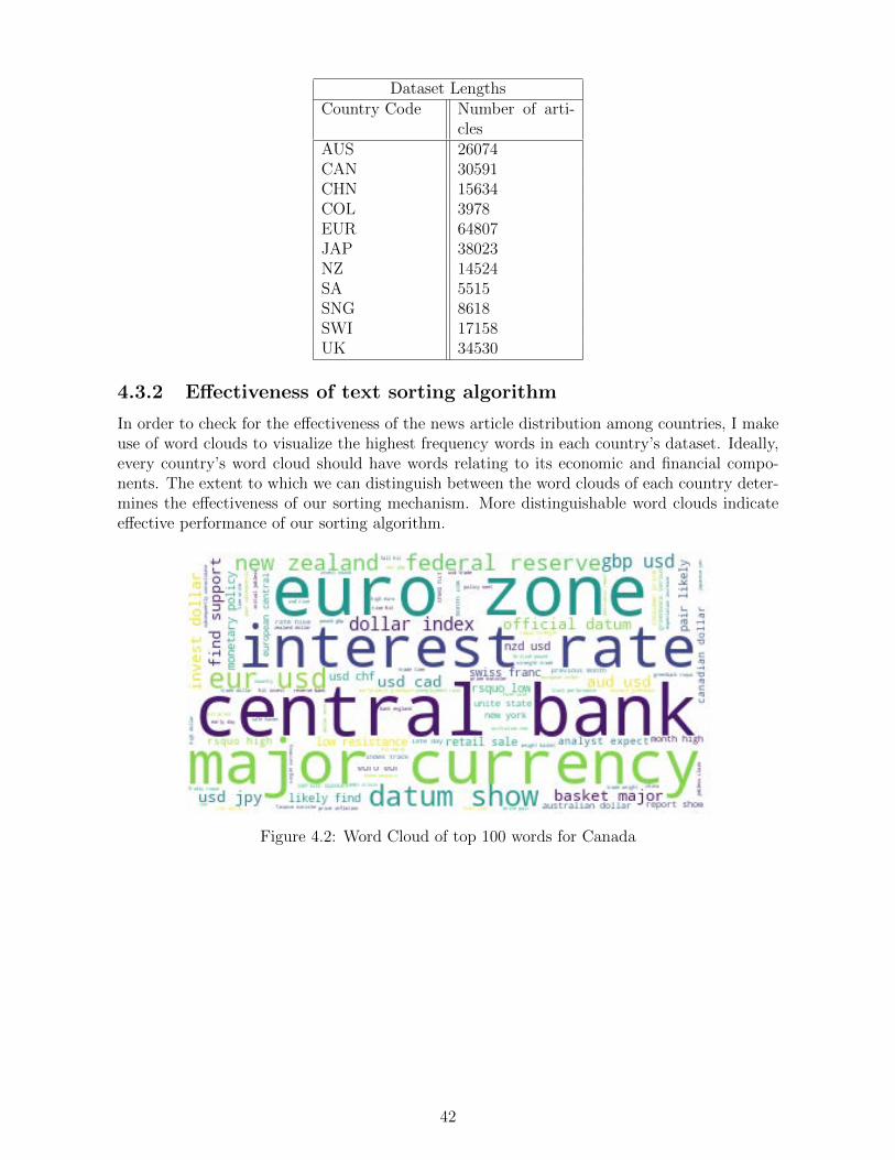
In order to check for the e↵ectiveness of the news article distribution among countries, I makeuse of word clouds to visualize the highest frequency words in each country’s dataset. Ideally,every country’s word cloud should have words relating to its economic and financial compo-nents. The extent to which we can distinguish between the word clouds of each country deter-mines the e↵ectiveness of our sorting mechanism. More distinguishable word clouds indicatee↵ective performance of our sorting algorithm.

Figure 4.2: Word Cloud of top 100 words for Canada

42

Figure 4.3: Word Cloud of top 100 words for China

Figure 4.4: Word Cloud of top 100 words for Japan

The figures above show word clouds for Canada, China, and Japan respectively. Oursorting mechanism is e�cient if word cloud for each country can easily be distinguished. This,however, does not appear to be the case. The word clouds for China, Canada and Japan do notappear to vary greatly. This indicates that our sorting mechanism was not very e�cient. It isunderstandable that “interest rate” is the most frequent term but words like “Euro Zone” whichare not directly related to China and Japan’s currency should not occur in their respective wordclouds. Every country’s word cloud not only appears to have a mention of its own currencybut also that of other currencies. This leads to the introduction of noise in our textual datasetswhich can cause our sentiment model to misclassify one country’s sentiment with that ofanother. The word clouds above show that our strategy for sorting text by country was notvery e↵ective. This can influence our sentiment analysis results as our datasets might notbe representative of the countries being considered. It will be vital to reconsider our textsorting mechanism if the exchange rate directional forecasting results with textual data are notsignificant.

43

4.4 Sentiment Analysis

Sentiment Analysis is a subfield of Natural Language Processing that aims to determine whethera piece of text is negative, positive or neutral in tone. This is also known as opinion mining oremotion AI. Sentiment Analysis helps us convert unstructured text data into structured datathat can then be used to train a model. Sentiment analysis is widely used in asset pricing andfinancial market analysis because of the importance of expectation component in predictingdi↵erent financial variables such as exchange rates and stock prices. News articles and socialmedia are known to be one of the major drivers of expectation in the financial markets. Machinelearning algorithms cannot directly understand a news or social media article. They requiresentiment analysis or some other similar natural language processing technique to covert datainto a processable format. Sentiment analysis informs us about the polarity of a news paperarticle which can then be used to determine the directional change in exchange rate or anyother asset prices. Sentiment Analysis can be applied at di↵erent scope levels:

• Document Level: sentiment analysis used to obtain the tonality of a complete docu-ment, article or paragraph.

• Sentence Level: sentiment analysis used to obtain the tonality of a single sentence.

• Sub-sentence Level: sentiment analysis used to obtain the tonality of sub expressionswithin a single sentence.

In my analysis, I am going to use document level sentiment analysis as the text datasetconsists of daily foreign exchange news articles. In order to bring everything to daily frequencyfor predicting directional change, I combined all articles issued on the same day into a singledocument. This makes sure that we have one document for each day and the sentimentanalysis for that document would represent the overall tonality of that particular trading day.This overall sentiment can then be used to predict future daily directional change in exchangerates.

4.4.1 Methods for Sentiment Analysis

There are many methods and algorithms that can be used to implement sentiment analysissystems on textual data. They can be classified as follows:

• Rule based systems perform sentiment analysis based on a set of manually determinedrules. A basic rule based system usually works from the face of a predetermined dictionaryof positive and negative words. The dictionary is used to identify the number of positiveand negative words occurring in a document. If the number of positive words are greaterthan the number of negative words then the document is classified as positive or else itis given a negative sentiment. A neutral sentiment score is given when the number ofnegative and positive words in a document are the same. This is the basic form of rulebased sentiment analysis. Other advanced rule based sentiment analysis use di↵erenttechniques such as assigning di↵erent weights to specific positive and negative words i.e.words that are extremely negative or positive are given more weight in a document thanthose that are more neutral. This helps make our model more dynamic as all negativeand positive words in our dictionary are not treated the same.

• Automatic systems rely on machine learning and deep learning techniques to learn fromtextual data. Unlike Rule based systems, they do not depend on manually crafted rulesfor sentiment analysis. In the case of automatic systems, the sentiment analysis task

44

is usually modeled as a classification task. This means that for automatic systems itis important to use an already pre-labeled training text dataset. The training datasetis used to fit a machine learning classification model such as Support Vector Machines,Neural Networks, or Logistic Regression. These trained models are then used to predictthe tonality of new unstructured text data that does not have any labels. The imagebelow shows how the training and prediction process of automatic systems for sentimentanalysis work:

Figure 4.5: Training and Prediction Process of Automatic Systems for Sentiment Analysis

During the training process of automatic systems, the textual data is considered as inputwhile the sentiment labels (positive, negative, and neutral) are considered as labels. Thelabels and text data is split into a training and test set in order to check for overfittingafter the model has been created. The text data is passed through the feature extractorbefore being fed into the machine learning algorithm. The feature extractor executesthe text preprocessing tasks by cleaning the textual dataset and using text to vectorconversion. Once the training dataset is in vector format, it is fed into the machinelearning classification algorithm along with its respective labels. After training the model,we use the test dataset to check for the out of sample performance of our machine learningalgorithm. Checking our model with a test dataset helps us make sure that our model isgeneralizable and not overfitting to the training dataset. After a suitable model has beendeveloped, we can use it to predict the labels of new unstructured textual data. Nowwe can use our model to predict the tonality of any new text documents. Deep learningautomatic systems work best for sentiment analysis if provided with huge training and testdatasets. Most people do not train their own automatic systems for sentiment analysis asit is very time consuming and computational expensive to train a deep learning sentimentanalysis model. Instead most of the automatic systems used today are pre-trained bylarge data science and Artificial Intelligence corporations.

• Hybrid systems combine both the rule based and automatic approaches. Hybrid systemscan gain higher precession and accuracy by combining the best of both worlds.

45

4.4.2 Models for Sentiment Analysis

In this section, I am going to discuss the models that I used for sentiment analysis on the newsarticles dataset. A combination of rule based and automatic sentiment analysis systems areused in an e↵ort to identify the best sentiment extraction technique for predicting short rundirectional change in exchange rates. Following is the list of sentiment analysis techniques thatwere used:

• Tonality Dictionary is a rule based system with 231 positive words and 102 negativewords in its dictionary. The sentiment analysis dictionary for this model is adapted fromthe paper ’What’s the Story? A New Perspective on the Value of Economic Forecasts’where the authors use it to measure the degree of optimism and pessimism regardingFederal Reserve Board forecasts published in the Greenbook (Sharpe, Sinha, & Hollrah,2017). The model uses a tf-idf weighting scheme along with the dictionary of positiveand negative words for conducting sentiment analysis on foreign exchange news articles.A sentiment score that is greater than 0 is considered to be positive while anything lessthan 0 is considered negative. A score of exactly 0 is considered to be neutral (which israrely the case.)

• VADER stands for Valence Aware Dictionary and sEntiment Reasoning. It is an opensource pre-trained algorithm that works o↵ a simple rule based model for conductingsentiment analysis. It was created and optimized for sentiments expressed on socialmedia like twitter, online news, movie/product reviews etc. Furthermore, VADER is alsoable to include sentiments for emoticons (e.g. :D), acronyms (e.g. LoL) and slang. Idecided to use VADER for sentiment analysis on FOREX news articles because of itsreputation for performing well on online media including news articles. The compoundscore in VADER’s result is an aggregate of negative, positive and neutral sentiment scoresof a text. If the compound score of a document is greater than or equal to 0.05, it isconsidered to be positive. On the other hand, if the compound score of a document isless than or equal to -0.05, it is considered to be negative. Anything between -0.05 to0.05 is considered neutral.

• TextBlob is a python package that can be used for sentiment analysis. It is a rule basedsystem that works well with negation and modifier words. This means that it is able toclassify “great” as positive while “not great” as negative. It also understands modifierswhich means that it will assign a higher positive sentiment score to “very great” than“great”. It ignores one letter words in its sentiment phrases which means that sentenceslike “not a very great” will be assigned the same negative sentiment score as “not verygreat.” Lastly, it also ignores any words that does not exist its dictionary. This meansthat it will assign the same negative sentiment score to “not a very great calculation”as it will to “not a very great”. I decided to use it as one of my models for sentimentanalysis because of its capacity to understand di↵erent text structures that play a role intonality extraction. A sentiment score that is greater than 0 is considered to be positivewhile anything less than 0 is considered negative. A score of exactly 0 is considered tobe neutral (which is rarely the case.)

• Harvard IV-4 Dictionary is a tonality dictionary developed by Harvard Universitythat is most widely used for sentiment analysis as it contains a vast list of positive andnegative words. I used the dictionary to develop a rule based system that assigns a scoreof greater than 0 for positive sentiment, a score of less than 0 for negative sentiment, anda score of 0 for neutral sentiment.

46

• Loughran and Mcdonald (LM) Dictionary is a dictionary developed specificallyfor the accounting and financial domain. According to Loughran and McDonald (2011),applying a general sentiment word list to accounting and financial documents can lead tohigh rate of misclassification (Loughran & McDonald, 2011). It is for this reason that theydeveloped a custom financial dictionary of positive and negative words. They also addedan uncertainity word list that attempts to measure the general notion of imprecision.The financial dictionary contains 2339 negative words and 353 positive words. I usedthe LM dictionary to develop a rule based system that assigns a score of greater thatn 0for positive sentiment, a score of less than 0 for negative sentiment, and a score of 0 forneutral sentiment.

• Aggregate Sentiment system determines the sentiment of an article by averaging thesentiment score of all five models discussed above. The aggregate sentiment systems isan ensemble method that aims to tap into the strengths of all previous models. Ensemblemodels are meta-algorithms that combine di↵erent machine learning techniques into anoverall model that aims to reduce variance, bias or improve predictions. The aggregatemodel was developed based on the hypothesis that a combination of our models will per-form better than each individual model. To calculate tonality, it averages the sentimentscore of the previous five models: tonality dictionary model, vader, textblob, harvard IV-4 dictionary model, and Loughran and Mcdonald dictionary model. It assigns a positivesentiment score to any document that has been classified as positive by majority of themodels. Likewise, any document that has been classified as negative by 3 or more sen-timent algorithms will be classified as negative. The same condition holds for assigningneutral sentiment to a piece of text.

4.4.3 Results

This section shows the accuracy of di↵erent sentiment models in predicting the directionalchange in exchange rates at varying lagged intervals. A binary variable for directionalchange in exchange rate is created. A positive percentage change in exchange rate isgiven a value of 1, while a negative percentage change in exchange rate is given a valueof 0. Lags for the directional change in exchange rate are in daily frequency rangingfrom 0 to 30. A lag to 0 checks for whether a sentiment model can predict the same daydirectional change in exchange rate, while a lag of 30 checks for whether a model canpredict one month ahead directional change in exchange rate.The number of accuratepredictions of the sentiment model is calculated by adding up the number of times thelagged directional change in exchange rates is same as the sentiment score predicted bythe model. Afterwards, the accuracy percentage of the model is calculated by dividingthe number of accurate predictions by the total length of our dataset and multiplying theanswer by 100. The figures below show the accuracy scores of all our sentiment modelsin predicting the directional change in each currency’s exchange rate:

47

Figure

4.6:

Accuracy

Score

ofTon

alityDiction

aryMod

elat

VaryingDaily

Intervals

48

Figure

4.7:

Accuracy

Score

ofVADER

Mod

elat

VaryingDaily

Intervals

49

Figure

4.8:

Accuracy

Score

ofTextB

lobMod

elat

VaryingDaily

Intervals

50

Figure

4.9:

Accuracy

Score

ofHarvard

IV-4

Diction

aryMod

elat

VaryingDaily

Intervals

51

Figure

4.10:Accuracy

Score

ofLM

Diction

aryMod

elat

VaryingDaily

Intervals

52

Figure

4.11:Accuracy

Score

ofAggregate

Mod

elat

VaryingDaily

Intervals

53

The results of the sentiment model can also be viewed with the following app: https://asaficontact.shinyapps.io/fx sentiment/. Di↵erent models seem to perform betterfor di↵erent countries. It is interesting to see how most of the models get their lowestaccuracy score when trying to predict directional change in Colombia’s exchange rate,while, the Loughran and Mcdonald dictionary model, on the other hand, appears to pre-dict it with a high accuracy of about 60 percent. There seems to be no fixed relationshipbetween the lagged interval for directional change in exchange rate and the accuracyscore. Di↵erent country models seem to perform better at varying lagged intervals. Forsome countries, a model performs well at small lag values, while in case of others, thesame model performs better at larger lag value.

Combining sentiment scores of di↵erent models into one aggregate model does not seemto significantly improve our accuracy in predicting the directional change in exchangerates. The aggregate sentiment model assigns equal weights to all other models’ tonalityscore when combining their results. This might cause the accurate model’s prediction tobe outweighed by the inaccurate ones if the number of models assigning an inaccuratesentiment score are greater than the ones assigning an accurate score. Using some formof dynamic weighting mechanism into the aggregate model might improve its accuracy.

Di↵erent models seem to outperform the random walk model for di↵erent countries atvarying lagged intervals. This means that their accuracy score for predicting directionalchange in foreign exchange rates is greater than 50%. A random walk model, on anequally distributed dataset, has an accuracy score of 50%. VADER seems to be the bestperforming sentiment model for all countries, while Harvard IV-4 Dictionary model andTextBlob seems to be the lowest accuracy models (failing to beat the random walk modelin predicting directional change in exchange rate for most countries.)

4.5 Discussion

This chapter evaluates the importance of text preprocessing for developing an e�cientsentiment analysis model. The results show that di↵erent sentiment models better predictthe directional changes in exchange rates of di↵erent countries. This means that di↵erentsentiment models should be used for predicting di↵erent countries’ directional change inexchange rates. For example, in case of Colombia, the Loughran and Mcdonald dictionarymodel appears to have the highest accuracy, while in case of Canada VADER seems tobe the best performing one. This variation might be explained by the fact that the listof negative and positive words explaining a currency’s market sentiment di↵ers basedon country. In our analysis of country specific word clouds, I find that the sorting bycountry mechanism, developed to classify news articles based on country, is not verye�cient. This might be causing some country sentiment models to perform worse thanthe Random Walk model as misclassification of news articles can introduce noise in thedataset. Developing a more e�cient sorting by country algorithm can further improvethe predictive power of our sentiment analysis models in predicting directional change inexchange rates.

54

Chapter 5

Conclusion

Grounded in macro-economic theory, this paper explores whether machine learning tech-niques can better predict the directional change in foreign exchange markets than theRandom Walk model. I started o↵ by analyzing Uncovered Interest Rate Parity (UIP)and how it fails to predict changes in exchange rates. Then, I used the interest rate ofdi↵erent countries to sort them into portfolios for carry trade. I also used supervised ma-chine learning techniques such as Support Vector Machines (SVM) and Artificial NeuralNetworks (ANN) to predict the directional change in foreign exchange excess returns.Finally, I used Natural Language Processing (NLP) and Sentiment Analysis to create avariable for currency risk premium and market expectation that can be used to predictdirectional change in exchange rates.

While testing for UIP, I found that it does not hold over the short and long run. A � valueof less than zero emphasizes the importance of currency risk premium in understandingthe changes in exchange rates. It also shows the existence of arbitrage opportunity inthe currency market. This means that traders can earn large profits over the short runby borrowing from low interest rate countries’ bond market and investing in that of highinterest rate countries’. I analyze the excess returns in carry trade market by creatinga simulation based on historical interest rate and exchange rate data for trading on amonthly or semi-annual basis. According to the results, the returns on carry trade startto reduce with an increase in the trading interval. This means that a well diversifiedcarry trade portfolio is more profitable over short trading intervals (daily or monthly)than longer trading intervals (semi-annual or annual).

According to the spanning hypothesis, the yield curve, its expectation and term premiumcomponent span all relevant information related to the economic performance of a coun-try. This means that we can understand the economic situation of a country by analyzingits bond market. Based on the spanning hypothesis, I use Principal Component Analysis(PCA) to extract the level, slope, and curvature of the yield curve and its components.Then, taking the resultant principal components, I use Support Vector Machines (SVM)and Artificial Neural Networks (ANN) to predict the directional change in foreign ex-change excess returns. Compared to the SVMs, the ANNs more accurately predict thedirectional change in the exchange rate excess returns over the short run. This di↵erenceis attributed to the ability of Artificial Neural Networks to learn abstract features fromraw data.

Finally, in the last chapter, I use sentiment analysis to evaluate the tonality of foreign

55

exchange news articles from investing.com to develop a variable for understanding cur-rency risk premium and market expectations in order to predict the directional changesin the exchange rates. The foreign exchange markets are quite sensitive to unanticipatednews and events. This means that we can develop a variable for understanding currencyrisk premium and market expectation by using sentiment analysis on financial news ar-ticles. In order to identify the model that most reliably captures the tonality of foreignexchange news articles, I use five di↵erent sentiment analysis models: Tonality model,VADER model, TextBlob model, Harvard IV-4 Dictionary model, and Loughran andMcdonald Dictionary model. The results show that di↵erent sentiment models betterpredict the directional changes in exchange rates of di↵erent countries. For example, incase of Colombia, the Loughran and Mcdonald dictionary model appears to have thehighest accuracy, while in case of Canada VADER seems to be the best performing one.Overall, the VADER sentiment model best captures the tonality of foreign exchange newsarticles for most countries in the dataset.

All in all, this research finds evidence that machine learning models can more accuratelypredict directional change in exchange rates than the RandomWalk model when the inputfeatures used to train the machine learning models are representative of the economicsituation of a country. Hence, using macro-economic and financial theory to developinput features that capture the most relevant characteristics of a country’s economy canhelp us understand short run movements in the foreign exchange markets.

56

References

Aggarwal, S., et al. (2013). The uncovered interest rate parity puzzle in the foreignexchange market. Leonard N. Stern School of Business, Department of Economics.

Bekaert, G., & Hodrick, R. J. (1992). Characterizing predictable components in excessreturns on equity and foreign exchange markets. The Journal of Finance, 47 (2),467–509.

Berg, K. A., & Mark, N. C. (2018). Measures of global uncertainty and carry-trade excessreturns. Journal of International Money and Finance, 88 , 212–227.

Burnside, C. (2011). Carry trades and risk (Tech. Rep.). National Bureau of EconomicResearch.

Bussiere, M., Chinn, M. D., Ferrara, L., & Heipertz, J. (2018). The new fama puzzle(Tech. Rep.). National Bureau of Economic Research.

Calomiris, C. W., & Mamaysky, H. (2019). How news and its context drive risk andreturns around the world. Journal of Financial Economics , 133 (2), 299–336.

Cenedese, G., Sarno, L., & Tsiakas, I. (2014). Foreign exchange risk and the predictabilityof carry trade returns. Journal of Banking & Finance, 42 , 302–313.

Fama, E. F. (1984). Forward and spot exchange rates. Journal of monetary economics ,14 (3), 319–338.

Galeshchuk, S., & Mukherjee, S. (2017a). Deep learning for predictions in emergingcurrency markets. In Icaart (2) (pp. 681–686).

Galeshchuk, S., & Mukherjee, S. (2017b). Deep networks for predicting direction ofchange in foreign exchange rates. Intelligent Systems in Accounting, Finance andManagement , 24 (4), 100–110.

Hansen, L. P., & Hodrick, R. J. (1980). Forward exchange rates as optimal predictorsof future spot rates: An econometric analysis. Journal of political economy , 88 (5),829–853.

Jin, F., Self, N., Saraf, P., Butler, P., Wang, W., & Ramakrishnan, N. (2013). Forex-foreteller: Currency trend modeling using news articles. In Proceedings of the 19thacm sigkdd international conference on knowledge discovery and data mining (pp.1470–1473).

Loughran, T., & McDonald, B. (2011). When is a liability not a liability? textualanalysis, dictionaries, and 10-ks. The Journal of Finance, 66 (1), 35–65.

Lustig, H., Stathopoulos, A., & Verdelhan, A. (2013). The term structure of currencycarry trade risk premia (Tech. Rep.). National Bureau of Economic Research.

Meese, R. A., & Rogo↵, K. (1983). Empirical exchange rate models of the seventies: Dothey fit out of sample? Journal of international economics , 14 (1-2), 3–24.

Menkho↵, L., Sarno, L., Schmeling, M., & Schrimpf, A. (2011). The risk in carry trades.VoxEU. org , 23 .

Patel, K., Mohamed, A., & van Vuuren, G. W. (2018). A regression and comparativestudy of united states and south african yield curves using principal component

57

analysis. South African Journal of Economic and Management Sciences , 21 (1),1–15.

Salem, M. B., Castelletti, B., Csullag, B., Danielsson, J., Macrae, R., Daoud, Z., . . .Sunderam, A. (n.d.). The spanning hypothesis and risk premia in long-term bonds.

Schumaker, R., & Chen, H. (2006). Textual analysis of stock market prediction usingfinancial news articles. AMCIS 2006 Proceedings , 185.

Sharpe, S. A., Sinha, N. R., & Hollrah, C. (2017). What’s the story? a new perspectiveon the value of economic forecasts.

Thu, T. N. T., & Xuan, V. D. (2018). Supervised support vector machine in predictingforeign exchange trading. International Journal of Intelligent Systems and Appli-cations , 10 (9), 48.

Wang, J., et al. (2008). Why are exchange rates so di�cult to predict? Economic Letter ,3 .

58