learning temporal nodes bayesian networks - inaoeemorales/papers/2013/2013... · learning temporal...

International Journal of Approximate Reasoning xxx (2013) xxx–xxx

Contents lists available at SciVerse ScienceDirect

International Journal of Approximate Reasoning

j o u r n a l h o m e p a g e : w w w . e l s e v i e r . c o m / l o c a t e / i j a r

Learning temporal nodes Bayesian networks

Pablo Hernandez-Leal, Jesus A. Gonzalez, Eduardo F. Morales, L. Enrique Sucar !

Instituto Nacional de Astrofísica, Óptica y Electrónica, Coordinación de Ciencias Computacionales, Luis Enrique Erro No. 1, Sta. María Tonantzintla,

Puebla, CP 72840, Mexico

A R T I C L E I N F O A B S T R A C T

Article history:

Available online xxx

Keywords:

Bayesian networks

Temporal reasoning

Learning

TemporalnodesBayesiannetworks (TNBNs)areanalternative todynamicBayesiannetworksfor temporal reasoningwithmuch simpler and efficientmodels in somedomains. TNBNs arecomposed of temporal nodes, temporal intervals, and probabilistic dependencies. However,methods for learning this type of models from data have not yet been developed. In thispaper, we propose a learning algorithm to obtain the structure and temporal intervals forTNBNs from data. Themethod consists of three phases: (i) obtain an initial approximation ofthe intervals, (ii) obtain a structure using a standard algorithm and (iii) refine the intervalsfor each temporal node based on a clustering algorithm.We evaluated themethodwith syn-thetic data from three different TNBNs of different sizes. Our method obtains the best scoreusing a combined measure of interval quality and prediction accuracy, and a competitivestructural quality with lower running times, compared to other related algorithms. We alsopresent a real world application of the algorithmwith data obtained from a combined cyclepower plant in order to diagnose temporal faults.

© 2013 Elsevier Inc. All rights reserved.

1. Introduction

Bayesian Networks [18] have been studied as a popular technique to deal with uncertainty. They have proven to besuccessful in different applications, such as medical diagnosis, crime risk factor analysis, sensor validation and customeranalysis [19,20,12,7], amongothers. However, traditional BayesianNetworks cannot dealwith temporal information. For thisreason, an extension called Dynamic Bayesian Networks (DBNs) [5] was introduced. DBNs can be seen as multiple slices of astatic BN over time, with links between adjacent slices. Nonetheless, these models may become quite complex, in particularwhen only a few important events occur over time.

Temporal Nodes Bayesian Networks (TNBNs) [1] are another extension of Bayesian Networks. They belong to a classof temporal models known as Event Bayesian Networks [10]. TNBNs were proposed to manage uncertainty and temporalreasoning. In a TNBN, each Temporal Node has intervals associated to it. Each node represents an event or state change ofa variable. An arc between two Temporal Nodes corresponds to a causal-temporal relation. One interesting property of thisclass of models, in contrast to Dynamic Bayesian Networks, is that temporal intervals can differ in number and size.

TNBNs have been used in diagnosis and prediction of temporal faults in a steam generator of a fossil power plant [1]. Theproblem is that there does not exist an algorithm to learn TNBNs models, so the model has to be obtained from externalsources such as domain experts. This can be a hard and prone to error task.

In this paper, we propose a learning algorithm to obtain the structure and the temporal intervals for TNBNs from data.The learning algorithm consists of three phases. In the first phase, we obtain an approximation of the intervals using asimple algorithm such as equal-width discretization (EWD) or a K-means clustering approximation. For the second phase,the BN structure is obtained with the structure learning algorithm introduced in [3]. The last step is performed to refine theintervals for each Temporal Node. This refinement uses the structure obtained in the previous step in order to improve the

! Corresponding author.

E-mail addresses: [email protected] (P. Hernandez-Leal), [email protected] (L.E. Sucar).

0888-613X/$ - see front matter © 2013 Elsevier Inc. All rights reserved.

http://dx.doi.org/10.1016/j.ijar.2013.02.011

Please cite this article in press as: P. Hernandez-Leal et al., Learning temporal nodes Bayesian networks, Int. J. Approx. Reason (2013),


2 P. Hernandez-Leal et al. / International Journal of Approximate Reasoning xxx (2013) xxx–xxx

intervals. For this, our algorithm obtains a number of possible sets of intervals for each configuration of the parents.We useda clustering approach to obtain the intervals, more specifically the algorithm models the data based on a Gaussian mixturemodel. Each component of the mixture corresponds to an interval. Given that our algorithm obtains different intervals, weapplied two pruning techniques to discriminate some intervals and to increase the efficiency of our algorithm. From theremaining intervals, our algorithm selects the set of intervals that maximizes the prediction accuracy.

We evaluate our algorithmwith three synthetic examples of TNBNs. The data was generated with different distributions.We compare our algorithmwith twobaselines: K-means and Equal-width discretization.We also compare it to the algorithmproposed in [9]. In the experiments, our algorithm obtains the best score in terms of a combined measure that takes intoaccount predictive accuracy and interval quality. Our algorithm also obtained lower running times. Finally, we present anapplication of the algorithmwith real data obtained from a power plant simulator in order to diagnose and predict temporalfaults.

The paper is organized as follows. In Section 2, the Temporal Nodes Bayesian Networkmodel is described. In Section 3, wepresent relatedwork about learning TNBNs. In Section 4, we introduce the proposed learning algorithm called LIPS (LearningIntervals-Parameters-Structure). In Section 5, we present an overview of experiments and measures used to evaluate ouralgorithm. The results of the algorithm with synthetic data are described in Section 6. In Section 7, we show the results ofapplying LIPS to a real world application. In Section 8, we present our conclusions and ideas for future research.

2. Temporal nodes Bayesian networks

Bayesian networks (BNs) are a successful model for dealing with uncertainty. However, static BNs are not suited to dealwith temporal information. For this reason, Dynamic Bayesian Networks [5,4] were introduced. In a DBN, a copy of a basemodel is made for each time stage. These copies are linked via a transition network. In this transition network it is commonthat only links between consecutive stages are allowed (Markov property). The problem is that DBNs can become verycomplex. This is unnecessary when dealing with problems for which there are only a few changes for each variable in themodel. Moreover, DBNs are not capable of managing different levels of time granularity. They usually have a fixed timeinterval between stages.

A Temporal Nodes Bayesian Network (TNBN) [1,10] is composed of a set of Temporal Nodes (TNs). TNs are connectedby edges, each edge represents a causal-temporal relationship between TNs. There is at most one state change for eachvariable (TN) in the temporal range of interest. The value taken by the variable represents the interval in which the eventoccurs. Time is discretized in a finite number of intervals, allowing a different number and duration of intervals for each node(multiple granularity). Each interval defined for a child node represents the possible delays between the occurrence of oneof its parent events (cause) and the corresponding child event (effect). Some Temporal Nodes do not have temporal intervals,these correspond to Instantaneous Nodes. Root nodes are instantaneous by definition [1]. Formally, a TNBN is defined asfollows.

Definition 1. A TNBN is defined as a pair B = (G, !). G is a Directed Acyclic Graph, G = (V, E). G is composed of V, a set ofTemporal and Instantaneous Nodes; E a set of edges between Nodes. The! component corresponds to the set of parametersthat quantify the network. ! contains the values !vi = P(vi|Pa(vi)) for each vi ! V; where Pa(vi) represents the set ofparents of vi in G.

Definition 2. A Temporal Node, vi, is defined by a set of states S, each state is defined by an ordered pair S = (", # ), where" is the value of a random variable and # = [a, b] is the interval associated, with an initial value a and a final value b.Thesevalues correspond to the time interval in which the state change occurs. In addition, each Temporal Node contains an extradefault state s = (“no change”, "), which has no interval associated. If a Node has no intervals defined for any of its states,then it receives the name of Instantaneous Node.

The following is an example based on [1], its corresponding graphical representation as a DBN and a TNBN are shown inFig. 1.

Example 1. Assume that at time t = 0, an automobile accident occurs, a Collision. This kind of accident can be classified assevere,moderate, ormild. To simplify the model, we will consider only two immediate consequences for the person involvedin the collision, Head Injury and Internal Bleeding. Head Injury can bruise the brain, and chest injuries can lead to internalbleeding. These three are instantaneous events that will generate subsequent changes, for example the Head Injury eventmight generate Dilated Pupils and unstable Vital Signs. Suppose that we gathered information about accidents occurredin a specific city. The information indicates that there is a strong casual relationship between the severity of the accidentand the immediate effect of the patient’s state. Additionally, a physician domain expert provided some important temporalinformation: If a head injury occurs, the brain will start to swell and if left unchecked the swelling will cause the pupils todilate within 0 to 60 min. If internal bleeding begins, the blood volume will start to fall, which will tend to destabilize vitalsigns. The time required to destabilize vital signs will depend on the bleeding severity: if the bleeding is gross, it will take



P. Hernandez-Leal et al. / International Journal of Approximate Reasoning xxx (2013) xxx–xxx 3

Fig. 1. A comparison between (a) DBN and (b) TNBN for a simple example. In this example, C=Collision, HI= Head Injury, IB= Internal Bleeding, DP= Dilated Pupils,

and VS=Vital Signs. In the DBN there are copies over time of the static network. In contrast, the structure of the TNBN is simpler and contains intervals in the

nodes in order to manage temporal information. For instance, it says that the pupils can be dilated in three possible time intervals depending on the severity of

the accident.

from 0 to 15 min; if the bleeding is slight it will take from 15 to 45 min. A head injury also tends to destabilize vital signs,taking from 0 to 15 min to make them unstable.

In Fig. 1(a) aDBNrepresentation ispresented for this example, theDBN ispresentedas a series of staticBNs connectedwithedges between them. For this example, we used a slice of 15 minutes, the maximum common divisor of the time intervals.In this case, the unrolled DBN contains five static BNs with a total of 25 nodes. This is a simple DBN which considers thefollowing assumptions: (i) a state only depends on the previous one, (ii) there are only links between the same variable atdifferent time slices.

In contrast, in Fig. 1(b) a TNBN for the same problem is presented. The model presents three instantaneous nodes:Collision, Head Injury and Internal Bleeding. These events will generate subsequent changes that are not immediate: DilatedPupils and unstable Vital Signs, that depend on the severity of the accident therefore they have temporal intervals associatedto them. This TNBN contains only five nodes, in contrast to the 25 nodes of the DBN.

In TNBNs, each variable represents an event or state change. So, only one (or a few) instance(s) of each variable is required,assuming there is one (or a few) change(s) of a variable state in the temporal range of interest. No copies of the model areneeded, and no assumption about the Markovian nature of the process is made. TNBNs can deal with multiple granularity,because the number and the size of the intervals for each node can be different.

3. Related work

There are several methods to learn BNs from data [17]. Unfortunately, the algorithms used to learn BNs cannot deal withthe problem of learning temporal intervals. Then, these cannot be applied directly to learn TNBNs.

To the best of our knowledge, there is only one previous work that attempts to learn a TNBN. [15] proposed a methodto build a TNBN from a temporal probabilistic database. The method obtains the network structure from a set of temporaldependencies in a probabilistic temporal relational model (PTRM). A Temporal Relational Model (TRM) is a relational modelwith temporal attributes. A PRTM is a TRM extended by adding a probabilistic attribute p. In order to build the TNBN, theyobtain a variable ordering that maximizes the set of conditional independence relations implied by a dependency graphobtained from the PTRM. Based on this order, a directed acyclic graph corresponding to the implied independence relationsis obtained. This graph represents the structure of the TNBN. They assume a known probabilistic temporal relational model




from the domain of interest, which is not always known. Building this PTRM can be as difficult as building a TNBN, and theydo not learn the temporal intervals of each node. In contrast, our approach constructs the TNBN directly from data and italso learns the intervals for each node.

Algorithm 1: Algorithm introduced in [9]

Data: An initial discretization.Result: A local optimal discretization.Push all continuous variables onto a queue Q1while Q is not empty do2

Remove first element X from Q3Compute new discretization policy for X4if score with new discretization < score with old discretization then5

Use new discretization6For all Y interacting with X , if Y /! Q , push Y onto Q .7

end8end9return Discretization policy10

Another related work is described in [9]. Here the idea is to learn the structure of a BN while discretizing the continuousvariables. For this, a score based on the Minimum Description Length [14] is proposed. The score takes into account theparameters, the structure, and the discretization policy. With this score, a search for the best discretization is done for eachcontinuous variable. The algorithm scores the Ni midpoints of each variable. Then, a top-down refinement is performedusing a greedy search strategy. Depending on the network structure, this approach can become complex if the continuousvariables interact with each other (if a variable does not interact with other variables it can be discretized separately). Forthis reason, the approach consists on discretizing one variable at a time and leave the rest as discrete and fixed. Therefore, thealgorithm does guarantee finding an optimal discretization. In order to learn the structure of the network, all the nodes arefirst discretizedand later, the structure learningalgorithm is applied. This alternatingprocess is performeduntil convergence.

The algorithm presented in [9] for discretizing several variables is shown in Algorithm 1, and it proceeds as follows. First,it pushes all continuous variables onto a queue Q , then a cycle starts while Q is not empty. A discretization is obtained forthe considered variable in a greedy way. Then, the interacting variables are pushed onto Q . The algorithm finishes whenthe queue is empty. This algorithm was proposed to learn the structure of a BN while discretizing continuous variables.This problem is similar to the one of learning the structure and the intervals for the TNBN thus we use it as a comparisonfor our experiments: the continuous variables will represent the temporal nodes of the TNBN, the result will be a BN withsome discretized nodes that will correspond to the intervals. Thus, the algorithm can be applied as usual. A problem withthis algorithm is that it may become too complex in cases where the continuous data is sparse since it has to obtain all themidpoints in the data. This may also happen if the network has many edges (several nodes interacting with each other). Incontrast, the LIPS algorithm is not directly affected by the data distribution.

4. Learning algorithm

In this sectionwe first present the interval learning algorithm that is applied for each Temporal Node.We initially assumethatwe have a defined structure. Later, we present thewhole learning algorithm. The proposed algorithmobtains a structureand sets of intervals for the TNBN. The algorithm assumes that the root nodes are instantaneous nodes and it obtains a finitenumber of non overlapping intervals for each temporal node. Our approach uses the times (delays) between parent eventsand the current node as input for learning the intervals. With this top-down approach the algorithm is guaranteed to arriveat a local maximum in terms of predictive score.

4.1. Interval learning

Initially, we assume that the events that we can model as TNs follow a known distribution. With this idea, we can usea clustering algorithm to work with temporal data. Each cluster corresponds, in principle, to a temporal interval. The firstapproximation of the algorithm ignores the values of the parent nodes. Later, we refine the method by incorporating theparent nodes configurations.

4.2. First approach: independent variables

Our approach uses a Gaussian mixture model (GMM) to perform an approximation of the data, therefore we can usethe Expectation-Maximization (EM) algorithm [6] to obtain the parameters of the GMM. EM works iteratively using twosteps: (i) The E-step tries to guess the parameters of the Gaussian distributions, (ii) the M-step updates the parameters ofthe model based on the previous step. By applying EM, we obtain a number of Gaussians (clusters), specified by their mean




Table 1

Initial sets of intervals obtained for node Dilated Pupils. There

are three sets of intervals for each partition.

Partition Intervals

Head Injury=true [11#35][11#27][32#53][8#21][25#32][45#59]

Head Injury=false [3#48][0#19][39#62][0#14][28#40][47#65]

and variance. For now, assume that the number of temporal intervals (Gaussians) is given. For each TN we have a dataset ofpoints over time, and these are clustered using GMM, to obtain k Gaussian distributions. Based on the parameters of eachGaussian, the temporal intervals are initially defined as: [µk # $k, µk + $k].

Now we deal with the problem of finding the number of intervals. The ideal solution has to fulfill two conditions: (i) thenumber of intervals must be small in order to reduce the complexity of the network, and (ii) the intervals should yield goodestimations when performing inference over the network. Based on the above, our approach uses the EM algorithm varyingthe parameter for the number of clusters from 1 to %, where % is the highest value (for the experiments in this paper we used% = 3).

In order to select the best set of intervals, we evaluate the network. This corresponds to an indirectmeasure of the qualityof the intervals. In particular, we used the Brier Score [2] to measure the predictive accuracy of the network. The selected setof intervals for each TN are those that maximize the Brier Score. The Brier Score is defined as

BS = 1

n

n!

i=1

(1 # Pi)2

where Pi is the marginal posterior probability of the correct value of each node given the evidence. The BS is obtained byinstantiating a random subset of variables in the model, predicting the unseen variables, and obtaining the BS for thesepredictions.

4.2.1. An exampleWe will illustrate the process of using the first approximation for obtaining the intervals for the TN Dilated Pupils of Fig.

5(a). We can see that its parent node (Head Injury) has two configurations, true and false. Thus, we separate the temporaldata of Dilated Pupils in two partitions, one for each configuration of the parent node. Then, for each partition we apply thefirst approximation of the algorithm. We apply the EM algorithm to get a Gaussian mixture with parameters 1, 2 and 3 asthe number of clusters. That give us six different sets of intervals, as we show in Table 1. Then we obtain the Brier Score foreach set of intervals to measure its quality and select the set of intervals with the best score.

4.3. Second approach: considering the network topology

Now we will construct a more accurate approximation. For each Temporal Node we use the configurations of the parentnodes. The number of configurations of each node X is qX = "

Y!Pa(X) |sY | (the product of the number of states of the parentsnodes).

Formally, we construct partitions of the data (temporal data), one partition for each configuration. Then, we get binarycombinations taking partitions pi,pj (see Fig. 2(a)). This will yield q(q # 1)/2 different binary combinations. For each pi, pjthe first approximation of the algorithm is applied. Therefore, we obtain % intervals for each partition (see Fig. 2(b)). Then, acombination of the sets of the first approximation is performed (see Fig. 2(c)), this will generate %2 sets of intervals for eachpair pi, pj . Lastly, these intervals need to be adjusted (see Fig. 2(d)) in order to be defined in an exhaustive and mutuallyexclusive set of intervals, this adjustment is performed by Algorithm 2.

Algorithm 2 performs a cycle, for each set of intervals we sort them by its starting point. Then, we check if there isan interval contained in another interval. While this is true, the algorithm obtains an average interval, taking the aver-age of the start and end points of the intervals and replacing these two intervals with the new one. Next, we refine theintervals to be continuous by taking themean of two adjacent values and finally a rounding operation is performed. A graph-ical representation of the interval learning algorithm is presented in Fig. 3. An example of this algorithm is presented inSection 4.3.2.

As in the first approximation, the best set of intervals for each TN is selected based on the predictive accuracy in termsof the BS. However, when a TN has as parents other Temporal Nodes (an example of this situation is illustrated in Fig. 5(b)),the state of the parents is not initially known. For this reason, we cannot directly apply the second approximation. In orderto solve this problem, the intervals are sequentially selected in a top-down fashion according to the TNBN structure. That is,we first select the intervals for the nodes in the second level of the network. Once these are defined, we know the values ofthe parents of the nodes in the third level. Then, we can find their intervals; and so on, until the leaf nodes are reached.




Fig. 2. Graphical description of the interval learning algorithm: (a) binary partitions that correspond to the configurations of the parent nodes are selected, (b) for

each partition the first approximation to generate different sets of intervals is applied (between 1 and 3 in this paper), (c) the intervals generated in the previous

step are combined, (d) these intervals are adjusted using Algorithm 2.

Fig. 3. Graphical representation of the interval learning algorithm: (a) histogram of the temporal data, (b) Gaussians obtained by applying the EM algorithm, (c)

first approximation of the intervals using the parameters of the Gaussians, (d) final intervals of the algorithm.




Algorithm 2: Algorithm to adjust the intervals

Data: Array of intervals setsResult: Array of adjusted intervalsfor Each set of intervals s do1

sortIntervalsByStart(s)2while Interval i is contained in Interval j do3

tmp=AverageInterval(i,j)4s.replaceInterval(i,j,tmp)5

end6for k = 0 to number of intervals in set s -1 do7

Interval[k].end=round ((Interval[k].end + Interval[k+1].start)/2)8end9

end10

Table 2

Final sets of intervals obtained for node Dilated

Pupils. The selected set of intervals that obtained

the best Brier Score is presented in bold.

Intervals node dilated pupils

[0#15][16#37][38#62][0#12][13#31][32#43][44#65][7#37][38#53][15#39][40#59][0#13][14#23][24#38][39#60]

4.3.1. PruningTaking the combinations and joining the intervals can become computationally expensive. The number of sets of intervals

for a node is in O(q2%2), where q is the number of configurations and % is the maximum number of clusters for the GMM.For this reason we used two pruning techniques for each TN to reduce the computation time.

The first pruning technique discriminates the partitions that contain few instances. For this, we count the number ofinstances in each partition, and if it is greater than a value

& = Number of instances

Number of partitions $ 2

the configuration is used, if not it is discarded.A second pruning technique is applied when the intervals for each combination are being obtained. If the final set of

intervals contains only one interval (no temporal information) or more than ' (producing a complex network), the set ofintervals is discarded. In section 6.1 we present some experiments to obtain the value of ' used in the rest of the paper.

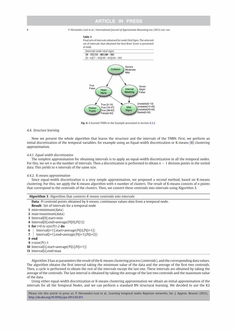
4.3.2. Revisited exampleWe had six different sets of intervals obtained by the first approximation for the TN Dilated Pupils, as we show in Table 1.

Then, we combine these sets of intervals for each partition with the other partitions. In this case, there could be 3 $ 3 = 9different sets of intervals, but some of these combinations are eliminated using the proposed pruning methods.

For example, we should merge the sets [11#35] and [3#48] because they correspond to different partitions, if we jointhem we get [11#35][3#48]. With this set we apply Algorithm 2. In this case when we sort them to get [3#48][11#35].The next thing to do is to check whether one interval is contained in another, this is true ([11#35] in [3#48]), then weobtain the average interval [7#41], this would be the final interval, however because of the pruning methods, this intervalwill not be added to the final list of intervals, since it is composed of only one temporal interval. The algorithm continuestaking [11#35] and [0#19][39#62]. If we join these intervals we get [11#35][0#19][39#62]. Applying Algorithm 2 wesort the intervals to obtain [0#19][11#35][39#62]. Here, no interval is contained in another so we skip the code inside thewhile statement. Thenwe refine the intervals to obtain [0#15][16#37][38#62], this set of intervals is added to the final listof intervals. The process continues with the rest of the nodes and we obtain the sets of intervals shown in Table 2.

This process is applied to each Temporal Node. To select the set of intervals for each node we apply the inferencetest (based on the maximization of the Brier Score) described in Section 4.2. In this case, the best set of intervals is:[0#15][16#37][38#62].

Applying the process to the remaining TN Vital Signs would yield the sets of intervals shown in Table 3. We present thebest set of intervals in the TNBN of Fig. 4.




Table 3

Final sets of intervals obtained fornodeVital Signs. The selected

set of intervals that obtained the best Brier Score is presented

in bold.

Intervals node vital signs

[0#13][13#40][40#50][0#6][7#29][30#43][44#50]

Fig. 4. A learned TNBN in the Example presented in Section 4.3.2.

4.4. Structure learning

Now we present the whole algorithm that learns the structure and the intervals of the TNBN. First, we perform aninitial discretization of the temporal variables, for example using an Equal-width discretization or K-means [8] clusteringapproximation.

4.4.1. Equal-width discretizationThe simplest approximation for obtaining intervals is to apply an equal-width discretization in all the temporal nodes.

For this, we set n as the number of intervals. Then a discretization is performed to obtain n # 1 division points in the sorteddata. This yields to n intervals of the same size.

4.4.2. K-means approximationSince equal-width discretization is a very simple approximation, we proposed a second method, based on K-means

clustering. For this, we apply the K-means algorithm with n number of clusters. The result of K-means consists of n pointsthat correspond to the centroids of the clusters. Then, we convert these centroids into intervals using Algorithm 3.

Algorithm 3: Algorithm that converts K-means centroids into intervals

Data: Pi centroid points obtained by k-means, continuous values data from a temporal node.Result: Set of intervals for a temporal nodemin=minimum(data)1max=maximum(data)2Interval[0].start=min3Interval[0].end=average(Pi[0],Pi[1])4for i=0 to size(Pi)-2 do5

Interval[i+1].start=average(Pi[i],Pi[i+1])6Interval[i+1].end=average(Pi[i+1],Pi[i+2])7

end8i=size(Pi)-19Interval[i].start=average(Pi[i],Pi[i+1])10Interval[i].end=max11

Algorithm3has as parameters the result of theK-means clusteringprocess (centroids), and the correspondingdata values.The algorithm obtains the first interval taking the minimum value of the data and the average of the first two centroids.Then, a cycle is performed to obtain the rest of the intervals except the last one. These intervals are obtained by taking theaverage of the centroids. The last interval is obtained by taking the average of the last two centroids and themaximum valueof the data.

Using either equal-width discretization or K-means clustering approximation we obtain an initial approximation of theintervals for all the Temporal Nodes, and we can perform a standard BN structural learning. We decided to use the K2




Table 4

Collected data to learn the TNBN of Fig. 5(a). For Dilated Pupils and Vital Signs the temporal data represents the minutes

after the collision occurred.

Collision Head injury Internal bleeding Dilated pupils Vital signs

Severe True Gross 14 20

Moderate True Gross 25 25

Mild False False – –

… … … … …

Severe True Gross [10–20] [15–30]

Moderate True Gross [20–30] [15–30]

Mild False False – –

… … … … …

algorithm [3], since K2 has as a parameter an ordering of the nodes, this ordering of the nodes affects the structure of thenetwork since it restricts the possible arcs in the following way. If a node xi precedes xj in the ordering, then structures inwhich there is an arc from xj to xi are not allowed. For learning TNBNs we can exploit this parameter and define an orderbased on domain information. For instance, for the medical example presented in Section 2, we have a partial ordering ofthe temporal events: {Collision}, {Head Injury, Internal Bleeding}, {Edema, Blood Pressure, Heart Rate}, and {Dilated Pupils,Shock}. Therefore, we can define a total ordering based on the partial one, this ordering is then used in the K2 algorithm.

Once thenetworkstructurehasbeenobtained,weapply the interval learningalgorithmdescribed inSection4.1.Moreover,this process of alternating interval learning and structure learning may be iterated. For the experiments presented in thispaper we only applied one iteration of the algorithm.

4.4.3. A complete exampleFirst assume we have data from accidents that is similar to the one presented in the upper part of Table 4. The first three

columns have nominal data, however, the last two columns have temporal data that represents the occurrence of thoseevents after the collision. Those two columns would correspond to Temporal Nodes of the TNBN. We start by applying theEWD algorithm in the numerical data, so it would yield results as the ones presented in lower part of Table 4.

Using the discretized data we can apply the K2 learning algorithm using the partial ordering of the temporal events:{Collision}, {Head Injury, Internal Bleeding}, and {Dilated Pupils, Vital Signs}. Now we have an Initial TNBN, however theobtained intervals are somewhat naive, so interval learning algorithmcanbe applied as presented in the examples in sections4.2.1 and 4.3.2. This process will learn a TNBN like the one presented in Fig. 4.

5. Evaluation on synthetic cases

In order to evaluate our algorithm, we considered three synthetic cases corresponding to the TNBNs presented in Fig. 5.In Fig. 5(a), a simple model of the consequences of a car accident is presented. This network contains two temporal nodesand five nodes in total. In Fig. 5(b) an expanded model of the car accident is presented, it contains five temporal nodes andeight nodes in total. The third TNBN is shown in Fig. 5(c) and it corresponds to a TNBN used to diagnose faults in a subsystemof a fossil power plant [10], it contains 10 temporal nodes and 14 nodes in total.

Given that we know the original structure, parameters, and intervals of the reference TNBNs, we can use it to comparethe results of our algorithm. The idea is to sample the fully specified TNBN to generate data that reflects the model and theintervals. Then, we can use that data to reconstruct the model with the proposed algorithm. For the data that represents theintervals, we perform two experiments. In the first one, data was generated by a normal distribution over the intervals withparameters

µ = Interval_Start + Interval_End

2

$ = Interval_End # Interval_Start

2

For the second test, the data was generated with a uniform distribution over the intervals. The intervals used to generatethe data are the same as those shown in Fig. 5.

In the experiments, we compared the proposed algorithm (LIPS) and the algorithm introduced in [9] (F-G). As baselineswe used an Equal-Width discretization (EWD) and a K-means approximation (K-M) (presented in Section 4.4) for learningthe intervals for the Temporal Nodes.

5.1. Evaluation measures

Three different aspects of the TNBNs were evaluated: the structure (the graph), the intervals, and the completemodel.




Fig. 5. Three TNBNs of different size used in the experiments: (a) small, (b) medium, (c) large.

5.1.1. Measures of structure qualitySince we have a reference network, the most common approach for evaluating the learned network is to compare

these networks. The learned network obtains a higher score as its degree of similarity with the reference network in-creases. For measuring the quality of the structure of the TNBNwith respect to the reference network, three measures wereused:

• The structural similarity (SS) [21], which is a score between 0 and 1 (maximum) that counts the similar edges witha reference network. Formally, let C be the adjacency matrix n $ n of graph G, let s(C) = #

i,j ci,j the sum of all the

components of matrix C. Even more, we define the conjunction$

of two adjacency matrices C and C% as D = C$

C%,with di,j = ci,j & c%i,j .The structural similarity for two graphs G and G% is defined as SS(G, G%) = s(C&C%)

s(C) , where C is the

adjacency matrix of G and C% is the adjacency matrix of G%.• The number of added directed edges (E+) with respect to the reference network.• The number of deleted directed edges (E#) with respect to the reference network.

The best network should obtain score 1 in structure similarity and 0 for edges deleted and added.

5.1.2. Measures of interval qualityThe main difference between TNBNs and standard BNs are the temporal nodes and their intervals. For this reason it is

important to evaluate their quality. For this, we used two measures.




• The relative temporal error (RTE). First we define the expected time as:

te = (tend + tini)/2

where tini and tend are the initial and final values of the interval, so the expected time is the average of them. The rangeof a temporal node T is the difference between the maximum and the minimum value of all the intervals in the node.The relative temporal error for a Temporal Node T with respect to the original value torig is defined as:

RTE = |te # torig |range(T)

this is the difference between the real event (original data) and the expected mean of the interval, normalized by therange of T .

• The number of intervals (# I) in the network.

The best model should obtain a value closer to 0 in temporal error because this would show that intervals are representativeof the data. A lower number of intervals is also desired to reduce the complexity of the network.

5.1.3. Global measuresFor evaluating the complete model our first measure is the Brier Score. The Brier score is defined as

BS = 1

N

N!

i=1

(1 # P(vi|e))2

this is the sum of the quadratic error inferred for a node vi with the given evidence e.For obtaining the BS for each learned network the following methodology was performed. For each instance, select a

random subset of nodes of size s; 1 ' |s| ' N # 1. Instantiate all the nodes selected with respect to the original data.Perform inference in the rest of the nodes (the ones not assigned). A perfect score for the BS will be a value of 0.

Inearlier experiments [11]weused themeasuresmentionedbefore, however the results obtained showed that the relativetime error and the Brier score were related in some way. We believe this happened due to the fact that some algorithmsobtained a small number of large intervals thus, yielding large temporal error, but with high predictive score (because theprobability of error was lower due to the larger intervals). Therefore, we propose another measure that combines relativetime error with the predictive score. The measure called Predictive Temporal Error (PTE) is defined as:

PTE = ( $ (RTE) + (1 # () $ (BS)

where RTE is the relative time error, and BS is the Brier Score. Both of these measures are normalized between 0 and 1 andtheir best result is 0. The same happens with PTE. For our experiments we decided to use ( = 0.5 to give the same weightto interval and prediction quality.

Even with this measure, the question of which is the best model remains open. We believe that the answer is related tothe application domain. For some domains we could need models to be very effective in terms of accuracy, even if it is acomplex model.

5.2. Measure of statistical significance

In order to evaluate if the results obtained by our algorithm were statistically significant the Kruskal–Wallis test [13]was performed. Kruskal–Wallis is a non-parametric test used to verify whether a group of data is generated from the samedistribution. This test does not assume normality of the data and it is an extension of the Mann–Whitney–Wilcoxon test forthree or more groups.

To apply this test the K samples are combined and arranged in increasing size order and given a rank number. Whenties occur, the mean of the available rank numbers is used. The rank sum for each of the K samples is calculated. The teststatistic is:

H =%

& 12

N(N + 1)

K!

j=1

R2i

nj

'

( # 3(N + 1) (1)

where: nj is the number of observations in group j, Rj is the rank sum of the j group. N is the size of the combined sample.The null hypothesis of equal means is rejected when H exceeds the critical value.

Using Kruskal–Wallis we know whether a pair of groups is significantly different or not, but we are not certain whichof those pairs of groups are. For this we can perform a pair comparison using the Bonferroni adjustment. For a simpleBonferroni adjustment we divide the p value to be achieved for significance by the number of paired comparisons to bedone. The number of total pairs is given by T = K(K # 1)/2, therefore for each pair comparison if the result is smaller than'kw/T , (where 'kw is the significance level) then it is significant.




Table 5

Results varying ' and the number of data points for the three reference TNBNs. BS is Brier Score, RTE is relative temporal

error and SS is structural similarity.

' Data

250 500 1000

BS RTE SS BS RTE SS BS RTE SS

Small TNBN

2 0.24 0.32 0.60 0.23 0.30 0.63 0.23 0.29 0.85

3 0.24 0.30 0.63 0.23 0.30 0.60 0.23 0.31 0.85

4 0.23 0.33 0.63 0.23 0.30 0.67 0.23 0.29 0.85

5 0.24 0.30 0.63 0.23 0.32 0.63 0.23 0.30 0.83

6 0.25 0.34 0.60 0.23 0.31 0.63 0.22 0.31 0.83

300 500 1000


Medium TNBN

2 0.21 0.30 0.81 0.22 0.30 0.83 0.21 0.28 0.96

3 0.21 0.30 0.88 0.20 0.29 0.94 0.22 0.29 0.94

4 0.21 0.30 0.88 0.21 0.29 0.92 0.21 0.30 0.96

5 0.22 0.30 0.80 0.20 0.31 0.85 0.22 0.31 0.79

6 0.22 0.30 0.79 0.20 0.30 0.77 0.21 0.32 0.77

500 750 1000


Large TNBN

2 0.13 0.22 0.18 0.17 0.22 0.25 0.17 0.23 0.31

3 0.16 0.22 0.18 0.17 0.22 0.25 0.16 0.21 0.35

4 0.16 0.23 0.18 0.16 0.22 0.25 0.16 0.22 0.35

5 0.13 0.22 0.17 0.13 0.24 0.22 0.19 0.24 0.29

6 0.13 0.22 0.17 0.14 0.25 0.23 0.20 0.23 0.29

6. Experiments

The experiments were performed using synthetic data obtained from three different TNBNs of different sizes: small,medium and large. 1 These are depicted in Fig. 5. These TNBNswere used for the experiments since they are similar in termsof parameters to the ones presented in [1,10], two of them represent a simple medical problem and the last one was usedin a real world application in a power plant.

6.1. Parameters

The LIPS algorithm makes use of different parameters such as ', the maximum number of intervals in the TNBN that isused during the pruning phase, % the maximum number of initial intervals, and & is the minimum value of the number ofinstances needed in a partition to be considered through the algorithm.

For the % parameter we decided to set % = 3 since this parameter has a direct effect on the complexity of the algorithm.

The parameter & = Number of instancesNumber of partitions$2

, was explained in Section 4.3.1.

For the ' parameter we performed different experiments with the three reference TNBNs. For each TNBN we varied theparameter from 2 to 6, we varied the number of data points considered and we evaluate the learned TNBNs with threemeasures: Brier Score, Relative Time Error and Structural Similarity. Each result, presents the average of 5 experiments usingdata with a Gaussian distribution and 5 experiments with a uniform distribution.

The results are summarized in Table 5, from which we can obtain the following conclusions. For the first TNBN the bestresults were obtained with ' = 4 since it obtained 6 of the best scores from the 9 measures. However, it is important tonote that the results do not vary considerably for the other values of '. For the second net, the best results are obtainedwith ' = 3 and 4, both obtaining 5 best scores. One interesting aspect to note is that the structural similarity measure isthe one that varies the most when ' changes. For the third net the best results are obtained with ' = 3, and the secondbest parameter is with ' = 4. One important observation is that the results with ' = 6 are the worst and the best resultsare obtained with ' = 3 and 4.

From these experiments, we decided to set ' = 4 since it obtained good results and also because we would like to keepa low number of intervals in the network.

1 We consider a TNBN containing at most 5 nodes to be small, a TNBN containing between 5 and 10 nodes to be medium andmore than 10 nodes is considered

large.




Table 6

Results obtained for the TNBN of Fig. 5(a) using data generated by a Gaussian and uniform distribution. The average result

of varying the number of cases from 300 to 1000 is presented. For each row, the average of varying the number of initial

intervals from 2 to 4 is shown. Each experiment was repeated five times. E+ is the number of added edges, E# is the number

of deleted edges, BS is Brier Score, RTE is relative temporal error, SS is structural similarity, PTE is the predictive temporal

error and #Int is the total number of intervals in the TNBN. An ‘!’ is shown if the result of LIPS is significantly better than

EWD; ‘†’, if LIPS is significantly better than K-means and ‘§’, if LIPS is significantly better than Friedman’s algorithm.

Algorithm E+ E# SS BS RTE PTE #Int

Gaussian

EWD 0.15 1.50 0.700 ± 0.100 0.220 ± 0.015 0.307 ± 0.009 0.264 ± 0.010 6.00

K-M 0.03 1.50 0.700 ± 0.115 0.256 ± 0.011 0.317 ± 0.016 0.286 ± 0.010 6.00

F-G 0.33 1.41 0.717 ± 0.115 0.200 ± 0.013 0.335 ± 0.024 0.268 ± 0.014 3.73

LIPS 0.00§ 1.33! 0.733 ± 0.077 0.224 ± 0.004 0.285 ± 0.012§ 0.255 ± 0.005† 5.81

Uniform

EWD 0.16 1.50 0.700 ± 0.067 0.252 ± 0.006 0.325 ± 0.012 0.288 ± 0.008 6.00

K-M 0.24 1.41 0.717±0.084 0.256 ± 0.008 0.335 ± 0.017 0.296 ± 0.012 6.00

F-G 0.24 1.25 0.750 ± 0.100 0.239 ± 0.015 0.317 ± 0.012 0.268 ± 0.015 4.37

LIPS 0.01!†§ 1.25 0.750 ± 0.110! 0.230 ± 0.004† 0.303 ± 0.005† 0.268 ± 0.006† 4.45

6.2. Evaluating LIPS algorithm

For all the experiments, the following methodology was applied. Data was generated according to a reference TNBN, thetemporal data was generated using Gaussian and uniform distributions. Four different algorithms were evaluated in theexperiments:

1. Equal-Width Discretization (EWD). This algorithm is considered a baseline. It only uses an equal width discretizationto obtain intervals that correspond to the temporal nodes. It has as parameter the number of intervals to be generated.

2. K-means (K-M). This algorithm is also considered a baseline. It applies the K-means algorithm over the temporal data.Then, it applies an algorithm to transform the centroids into intervals for the temporal nodes. The algorithm has asparameter the number of clusters to obtain.

3. The algorithm presented in [9](F-G). This algorithm performs a discretization of the continuous data while learningthe structure. This algorithm was described in Section 3.

4. Our proposed algorithm (LIPS).

For the experiments we vary the number of cases. Each experiment was repeated five times. In the tables, the best resultsare presented in bold type. We applied statistical significance tests using the Kruskal–Wallis method with significance level'kw = 0.05. In the tables we show an ‘!’, if the result of LIPS is significantly better than EWD, a ‘†’ if LIPS is significantlybetter than K-means and a ‘§’ if LIPS is significantly better than Friedman’s algorithm.

6.3. Small TNBN

The first set of experiments was performed with the TNBN presented in Fig. 5(a). The objective of this experiment is toevaluate the algorithm on a very simple model.

In Table 6 the results of the experiments using a Gaussian and an Uniform distribution for obtaining the temporal dataare given. Each table presents the average results varying the number of cases using 300, 400, 500 and 1000 data cases.For each number of cases 4 rows are presented that correspond to the four algorithms being compared. Each row containsthe results of the seven measures presented before. For the structural similarity, Brier score, relative temporal error, andpredictive temporal error, the standard deviations are also presented. Some conclusions can be obtained from these results:

• LIPS obtained in average better scores than the two baseline algorithms.• LIPS algorithm obtained the best score in predictive temporal error with both distributions.• The Friedman’s algorithm obtained the lowest number of intervals in all the experiments in both distributions.• For structural similarity LIPS and Friedman’s algorithms obtained the best results. However, LIPS algorithm obtained a

lower number of added edges.

Additionally, in Table 7 a different view of the experiments is presented. In this case, the results are presented by ini-tialization. Column #I-I represents the number of initial intervals for the EWD, F-G, and LIPS algorithms. It represents thenumber of initial clusters for the K-M approximation. The results presented are the average of varying the number of datausing 300, 400, 500 and 1000 instances of data.

From the results, we can observe that for all the initializations LIPS and Friedman’s algorithms obtained better resultsthan the baseline algorithms. We can also observe that the results for the K-means approximation and EWD depend on theinitializations since a lower number of intervals yields to better results than an initialization with a larger number of initialintervals. This may happen due to the fact that the less intervals obtained, the larger they will be and therefore they could




Table 7

Results of the TNBN presented in Fig. 5(a) varying the number of initial intervals (#I-I).

#I-I Algorithm E+ E# SS BS TRE PTE #Int

Uniform

2 EWD 0.40 1.64 0.750 0.226 0.302 0.264 4.0

K-M 0.00 1.76 0.700 0.222 0.331 0.277 4.0

F-G 0.20 1.72 0.750 0.234 0.307 0.263 4.0

LIPS 0.00 1.36 0.750 0.231 0.301 0.267 5.9

3 EWD 0.00 1.80 0.700 0.259 0.338 0.298 6.0

K-M 0.00 1.60 0.750 0.241 0.325 0.269 6.0

F-G 0.60 1.72 0.750 0.230 0.303 0.268 3.6

LIPS 0.00 1.44 0.800 0.228 0.301 0.264 5.7

4 EWD 0.04 1.80 0.650 0.271 0.335 0.303 8.0

K-M 0.08 1.68 0.700 0.280 0.374 0.327 8.0

F-G 0.20 1.60 0.750 0.241 0.320 0.270 3.6

LIPS 0.00 1.36 0.700 0.231 0.307 0.272 5.7

Gaussian

2 EWD 0.08 1.44 0.700 0.195 0.289 0.242 4.0

K-M 0.00 1.60 0.700 0.215 0.292 0.253 4.0

F-G 0.20 1.60 0.700 0.204 0.348 0.276 4.2

LIPS 0.04 1.20 0.700 0.225 0.291 0.258 4.6

3 EWD 0.20 1.84 0.700 0.214 0.298 0.256 6.0

K-M 0.40 1.48 0.700 0.204 0.347 0.276 6.0

F-G 0.20 1.60 0.750 0.224 0.285 0.255 4.4

LIPS 0.00 1.60 0.750 0.221 0.275 0.248 4.4

4 EWD 0.20 1.84 0.700 0.250 0.334 0.292 8.0

K-M 0.32 1.60 0.700 0.286 0.333 0.310 8.0

F-G 0.32 1.40 0.700 0.193 0.311 0.252 4.6

LIPS 0.00 1.40 0.750 0.225 0.290 0.257 4.4

Table 8

Results obtained for the TNBN of Fig. 5(b) using data generated by a Gaussian and uniform distribution. The average result

of varying the number of cases with 300, 400, 500 to 1000 data instances is presented. For each row, the average of varying

the number of initial intervals from 2 to 4 is shown. Each experiment was repeated five times.


Gaussian

EWD 0.57 1.41 0.823 ± 0.071 0.223 ± 0.010 0.312 ± 0.004 0.261 ± 0.006 15.00

K-M 0.48 1.24 0.844 ± 0.092 0.243 ± 0.007 0.326 ± 0.010 0.285 ± 0.007 15.00

F-G 0.33 0.41 0.948 ± 0.040 0.195 ± 0.003 0.383 ± 0.004 0.289 ± 0.003 10.67

LIPS 0.24! 1.25! 0.875 ± 0.059 0.208 ± 0.006† 0.304 ± 0.011§ 0.257 ± †0.009 13.67

Uniform

EWD 0.63 0.75 0.906 ± 0.100 0.23 ± 0.006 0.300 ± 0.012 0.264 ± 0.008 15.00

K-M 0.71 0.75 0.906 ± 0.067 0.249 ± 0.008 0.300 ± 0.017 0.275 ± 0.012 15.00

F-G 0.24 0.66 0.917 ± 0.084 0.201 ± 0.015 0.320 ± 0.012 0.262 ± 0.015 10.00

LIPS 0.23!† 0.58 0.927 ± 0.114 0.201 ± 0.004† 0.286 ± 0.005 0.244 ± 0.006† 13.47

obtain better results in predictive score. It is important to note that LIPS algorithm is not significantly affected by varyingthe number of initial intervals.

6.4. Medium TNBN

The second set of experiments was performed using data obtained from the TNBN presented in Fig. 5(b). This TNBN isan extended model of the one presented in Fig. 5(a). It contains five temporal nodes. It is important to notice that in thisexample there are temporal nodes that have as parent only temporal nodes, therefore we will use the top-down approachproposed by LIPS.

In Table 8 the average results of the experiments are presented. Some conclusions can be obtained:

• LIPS algorithm obtained the best scores in PTE in both types of data (Gaussian and uniform).• For the Gaussian distribution, Friedman’s algorithm obtained the best score in structural similarity. However, for the

uniform distribution the results obtained for LIPS and Friedman are almost the same.• For the Gaussian distribution the results in structural similarity obtained by the K-means approximation and EWD are

worse than the ones obtained with the uniform distribution.• For both distributions, Friedman’s algorithm obtained the lowest number of intervals.




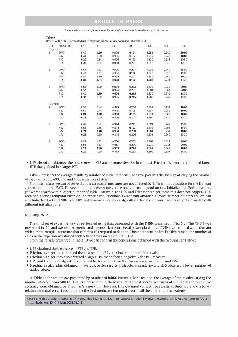
Table 9

Results of the TNBN presented in Fig. 5(b) varying the number of initial intervals (#I-I).


Uniform

2 EWD 0.40 0.60 0.906 0.194 0.286 0.240 10.00

K-M 0.44 0.68 0.906 0.197 0.287 0.242 10.00

F-G 0.20 0.84 0.906 0.196 0.320 0.258 10.80

LIPS 0.20 0.84 0.938 0.201 0.288 0.245 12.72

3 EWD 0.64 1.20 0.906 0.227 0.296 0.262 15.00

K-M 0.48 1.08 0.906 0.197 0.320 0.258 15.00

F-G 0.40 0.84 0.938 0.201 0.286 0.244 10.20

LIPS 0.20 0.84 0.938 0.197 0.285 0.241 13.28

4 EWD 0.68 2.20 0.906 0.262 0.302 0.282 20.00

K-M 0.52 1.60 0.906 0.291 0.310 0.301 20.00

F-G 0.40 0.80 0.906 0.205 0.320 0.270 11.00

LIPS 0.32 0.88 0.906 0.205 0.285 0.245 15.00

Gaussian

2 EWD 0.56 0.44 0.875 0.200 0.307 0.234 10.00

K-M 0.60 0.44 0.875 0.195 0.317 0.256 10.00

F-G 0.24 0.40 0.938 0.188 0.381 0.285 10.00

LIPS 0.24 0.60 0.906 0.207 0.300 0.254 13.20

3 EWD 0.48 0.92 0.844 0.215 0.319 0.267 15.00

K-M 0.68 0.88 0.844 0.197 0.392 0.295 15.00

F-G 0.24 0.40 0.938 0.208 0.304 0.257 10.00

LIPS 0.24 0.60 0.844 0.206 0.308 0.260 13.20

4 EWD 0.84 1.60 0.750 0.252 0.310 0.281 20.00

K-M 0.84 1.20 0.813 0.296 0.328 0.312 20.00

F-G 0.24 0.40 0.969 0.200 0.374 0.287 10.00

LIPS 0.20 0.60 0.875 0.210 0.304 0.257 14.00

• LIPS algorithm obtained the best scores in RTE and a competitive BS. In contrast, Friedman’s algorithm obtained largerRTE that yielded in a larger PTE.

Table 9 presents the average results by number of initial intervals. Each row presents the average of varying the numberof cases with 300, 400, 500 and 1000 instances of data.

From the results we can observe that the structural measures are not affected by different initializations for the K-meanapproximation and EWD. However, the predictive score and temporal error depend on this initialization. Both measuresget worse scores with a larger number of initial intervals. For LIPS and Friedman’s algorithms this does not happen. LIPSobtained a lower temporal error, on the other hand, Friedman’s algorithm obtained a lower number of intervals. We canconclude that for this TNBN both LIPS and Friedman are stable algorithms that do not considerably vary their results withdifferent initializations.

6.5. Large TNBN

The third set of experiments was performed using data generated with the TNBN presented in Fig. 5(c). This TNBN waspresented in [10] andwas used to predict and diagnose faults in a fossil power plant. It is a TNBN used in a real world domainwith a more complex structure that contains 10 temporal nodes and 4 instantaneous nodes. For this reason, the number ofcases in the experiments started with 500 and was increased until 3000.

From the results presented in Table 10 we can confirm the conclusions obtained with the two smaller TNBNs:

• LIPS obtained the best score in RTE and TPE.• Friedman’s algorithm obtained the best result in BS and a lower number of intervals.• Friedman’s algorithm also obtained a larger TPE that affected negatively the PTE measure.• LIPS and Friedman’s algorithms obtained better results than the K-means approximation and EWD.• Friedman’a algorithm obtained, in average, better results in structural similarity and LIPS obtained a lower number of

added edges.

In Table 11 the results are presented by number of initial intervals. For each one, the average of the results varying thenumber of cases from 500 to 3000 are presented. In these results the best scores in structural similarity and predictiveaccuracy were obtained by Friedman’s algorithm. However, LIPS obtained competitive results in Brier score and a lowerrelative temporal error, thus obtaining the best predictive temporal error in all the different initializations.




Table 10

Results obtained for the TNBN of Fig. 5(c) using data generated by a Gaussian and uniform distribution. The average result

of varying the number of cases from 500 to 3000 is presented. For each row, the average of varying the number of initial

intervals from 2 to 4 is shown. Each experiment was repeated five times.


Gaussian

EWD 0.55 12.91 0.193 ± 0.080 0.147 ± 0.007 0.301 ± 0.002 0.224 ± 0.003 30.00

K-M 0.56 12.41 0.224 ± 0.116 0.230 ± 0.006 0.318 ± 0.012 0.274 ± 0.008 30.00

F-G 0.60 11.99 0.250 ± 0.050 0.095 ± 0.012 0.373 ± 0.023 0.233 ± 0.009 20.00

LIPS 0.41 12.33! 0.229 ± 0.114! 0.145 ± 0.003 0.285 ± 0.002†§ 0.215 ± 0.001† 28.24

Uniform

EWD 0.62 11.66 0.271 ± 0.149 0.205 ± 0.007 0.296 ± 0.002 0.250 ± 0.004 30.00

K-M 0.87 11.66 0.271 ± 0.149 0.249 ± 0.011 0.296 ± 0.004 0.273 ± 0.004 30.00

F-G 0.60 11.00 0.312 ± 0.165 0.143 ± 0.011 0.322 ± 0.006 0.232 ± 0.006 20.00

LIPS 0.33† 11.16 0.302 ± 0.175!† 0.197 ± 0.006† 0.278 ± 0.002§ 0.238 ± 0.004† 25.20

Table 11

Results of the TNBN presented in Fig. 5(c) varying the number of initial intervals (#I-I).


Uniform

2 EWD 1.28 11.20 0.266 0.140 0.284 0.212 20.0

K-M 0.80 11.60 0.250 0.168 0.283 0.225 20.0

F-G 0.80 10.80 0.344 0.145 0.316 0.230 20.0

LIPS 0.60 12.00 0.328 0.178 0.277 0.228 25.4

3 EWD 0.33 10.33 0.281 0.209 0.292 0.251 25.0

K-M 0.67 10.50 0.297 0.165 0.328 0.246 25.0

F-G 0.17 9.50 0.313 0.197 0.278 0.238 16.6

LIPS 0.00 9.83 0.297 0.206 0.278 0.242 20.8

4 EWD 0.60 13.20 0.266 0.264 0.312 0.288 40.0

K-M 1.00 13.40 0.266 0.327 0.310 0.318 40.0

F-G 0.80 12.40 0.313 0.150 0.321 0.236 20.0

LIPS 0.40 11.60 0.281 0.208 0.279 0.243 25.2

Uniform

2 EWD 0.80 12.56 0.234 0.106 0.336 0.221 20.0

K-M 0.68 12.48 0.297 0.146 0.340 0.243 20.0

F-G 1.00 11.80 0.281 0.119 0.370 0.244 20.0

LIPS 0.56 12.08 0.250 0.147 0.287 0.217 28.4

3 EWD 0.32 13.32 0.203 0.143 0.284 0.213 30.0

K-M 0.44 12.88 0.234 0.094 0.354 0.224 30.0

F-G 0.40 12.40 0.266 0.145 0.285 0.215 20.0

LIPS 0.24 12.60 0.203 0.144 0.286 0.215 28.2

4 EWD 0.52 13.84 0.141 0.191 0.282 0.237 40.0

K-M 0.56 13.28 0.203 0.308 0.297 0.302 40.0

F-G 0.40 13.00 0.203 0.070 0.396 0.229 20.0

LIPS 0.44 12.56 0.234 0.146 0.282 0.214 28.1

6.6. General results

In Tables 12 and 13 a summary of the experiments using Gaussian and uniform distributions are presented. Each rowpresents the average results for the TNBN used for the four algorithms evaluated.

From these tables there are some conclusions:

• LIPS obtained the best results in RTE.• Friedman’s algorithm obtained the best results in BS and a lower number of intervals.• Since Friedman’s algorithm obtained the worse results in RTE, it had a significant effect in PTE.• LIPS obtained a competitive BS and the best RTE, therefore it obtained the best PTE.• EWD obtained competitive results in some experiments even when it is the simplest algorithm.• LIPS and Friedman’s algorithms obtained better results than the baseline algorithms in all the experiments.• Even when LIPS used the assumption that data is Gaussian when evaluated using a uniform distribution, it obtained

competitive results, even better than the baseline algorithms.




Table 12

Averages of the results with the three reference TNBNs using a Gaussian distribution to generate the temporal data.

Experiment Alg. E+ E# SS BS RTE PTE #Int

Small EWD 0.15 1.50 0.700 ± 0.100 0.220 ± 0.015 0.307 ± 0.009 0.264 ± 0.010 6.00

K-M 0.03 1.50 0.700 ± 0.115 0.256 ± 0.011 0.317 ± 0.016 0.286 ± 0.010 6.00

F-G 0.33 1.41 0.717 ± 0.115 0.200 ± 0.013 0.335 ± 0.024 0.268 ± 0.014 3.73

LIPS 0.00§ 1.33! 0.733 ± 0.077 0.224 ± 0.004 0.285 ± 0.012§ 0.255 ± 0.005† 5.81

Medium EWD 0.57 1.41 0.823 ± 0.071 0.223 ± 0.010 0.312 ± 0.004 0.261 ± 0.006 15.00

K-M 0.48 1.24 0.844 ± 0.092 0.243 ± 0.007 0.326 ± 0.010 0.285 ± 0.007 15.00

F-G 0.33 0.41 0.948 ± 0.040 0.195 ± 0.003 0.383 ± 0.004 0.289 ± 0.003 10.67

LIPS 0.24! 1.25! 0.875 ± 0.059 0.208 ± 0.006† 0.304 ± 0.011§ 0.257 ± †0.009 13.67

Large EWD 0.55 12.91 0.193 ± 0.080 0.147 ± 0.007 0.301 ± 0.002 0.224 ± 0.003 30.00

K-M 0.56 12.41 0.224 ± 0.116 0.230 ± 0.006 0.318 ± 0.012 0.274 ± 0.008 30.00

F-G 0.60 11.99 0.250 ± 0.050 0.095 ± 0.012 0.373 ± 0.023 0.233 ± 0.009 20.00

LIPS 0.41 12.33! 0.229 ± 0.114! 0.145 ± 0.003 0.285 ± 0.002†§ 0.215 ± 0.001† 28.24

Table 13

Averages of the results with the three reference TNBNs using a Uniform distribution to generate the temporal data.

Experiment Alg. E+ E# SS BS RTE PTE #Int

Small EWD 0.16 1.50 0.700 ± 0.067 0.252 ± 0.006 0.325 ± 0.012 0.288 ± 0.008 6.00

K-M 0.24 1.41 0.717±0.084 0.256 ± 0.008 0.335 ± 0.017 0.296 ± 0.012 6.00

F-G 0.24 1.25 0.750 ± 0.100 0.239 ± 0.015 0.317 ± 0.012 0.268 ± 0.015 4.37

LIPS 0.01!†§ 1.25 0.750 ± 0.110! 0.230 ± 0.004† 0.303 ± 0.005† 0.268 ± 0.006† 4.45

Medium EWD 0.63 0.75 0.906 ± 0.100 0.23 ± 0.006 0.300 ± 0.012 0.264 ± 0.008 15.00

K-M 0.71 0.75 0.906 ± 0.067 0.249 ± 0.008 0.300 ± 0.017 0.275 ± 0.012 15.00

F-G 0.24 0.66 0.917 ± 0.084 0.201 ± 0.015 0.320 ± 0.012 0.262 ± 0.015 10.00

LIPS 0.23!† 0.58 0.927 ± 0.114 0.201 ± 0.004† 0.286 ± 0.005 0.244 ± 0.006† 13.47

Large EWD 0.62 11.66 0.271 ± 0.149 0.205 ± 0.007 0.296 ± 0.002 0.250 ± 0.004 30.00

K-M 0.87 11.66 0.271 ± 0.149 0.249 ± 0.011 0.296 ± 0.004 0.273 ± 0.004 30.00

F-G 0.60 11.00 0.312 ± 0.165 0.143 ± 0.011 0.322 ± 0.006 0.232 ± 0.006 20.00

LIPS 0.33† 11.16 0.302 ± 0.175!† 0.197 ± 0.006† 0.278 ± 0.002§ 0.238 ± 0.004† 25.20

Table 14

Average and standard deviations of running times for F-G and LIPS algorithms for the three TNBNs used in the experiments.

The column # data shows the number of instances used for the small and the medium TNBNs, in parenthesis is shown the

number of instances used for the large TNBN. Each result is the average of 10 executions.

# Data Algorithm Small Medium Large

200 (250)F-G 6.04 ± 3.55 25.13 ± 5.10 44.24 ± 11.28

LIPS 6.65 ± 2.09 34.18 ± 4.09 31.99 ± 2.55

300 (500)F-G 6.18 ± 2.80 30.85 ± 3.96 134.21 ± 57.70

LIPS 5.82 ± 1.07 28.11 ± 4.02 37.03 ± 3.86

400 (1000)F-G 8.34 ± 2.72 46.79 ± 7.93 502.30 ± 53.03

LIPS 9.57 ± 0.80 34.84 ± 2.58 65.27 ± 4.96

500 (2000)F-G 12.01 ± 2.33 69.16 ± 6.47 2,275.99 ± 19.17

LIPS 9.24 ± 0.48 53.64 ± 2.41 95.19 ± 3.81

1000 (3000)F-G 37.81 ± 1.68 256.69 ± 9.15 6,342.38 ± 220.22

LIPS 14.63 ± 1.67 90.60 ± 2.65 591.19 ± 29.43

6.7. Temporal complexity experiments

In Table 14 the average and standard deviation of the running times (in seconds) of the LIPS and Friedman’s algorithmsare compared for different experiments varying the number of data instances for the three reference TNBNs shown in Fig.5. From the table we can make the following observations:

• In the small TNBN, the algorithm presented by Friedman obtained lower running times when the number of cases wasless than 500, however with 500 and 1000 cases, LIPS algorithm obtained lower running times.

• In the medium TNBN it happens the same behavior, when the number of cases was small (less than 400) Friedman’salgorithm obtained lower running times. As the number of cases increased, the same happens with the running times,therefore LIPS is more efficient with large number of data.

• In the large TNBN, even for a low number of cases, our algorithm obtained lower running times. Using 3000 cases forthis TNBN, LIPS was approximately 20 times faster in average than the algorithm presented by Friedman.




Fig. 6. Running times for the TNBNs of Fig. 5. The running times obtained by [9] are presented in black. The running times obtained by LIPS algorithm are presented

in light grey.

In Fig. 6 a graph showing the running times with respect to the number of data is presented. LIPS algorithm has a lowercurve in all the TNBNs than the one obtained by [9] algorithm. Some ideas that may give an intuition about the results ofthe algorithms are:

• Friedman’s algorithm has to evaluate all the mid-points in a dataset for each node to be discretized, this number can belarge depending of the dispersion on the data.

• Friedman’s algorithm has a cycle that will end when the queue of nodes is empty. However, when a discretization isobtained for a node, the last step of the algorithm is to add all the nodes that are in some way connected to that node.Therefore, on strongly connected TNBNs the algorithmwill have to add several nodes to the queue, increasing the runningtime.

7. A TNBN in a real application

Now, we present an example of a real domain application. We learned a TNBN in order to diagnose and predict temporalfaults in a subsystem of a combined cycle power plant.




Fig. 7. Schematic description of a power plant showing the feed-water and main steam subsystems. Ffw refers to feedwater flow, Fms refers to main stream flow,

dp refers to drum pressure, dl refers to drum level.

7.1. Application domain

A power plant mainly consists of three equipments: the steam generator (HRSG), the steam turbine and the electricgenerator. The steam generator, with the operation of burners, produces steam from the feed-water system. After the steamis superheated, it is introduced to the steam turbine to convert the energy carried out by the steam in work and finally inelectricity through the corresponding steam generator. A simplified diagram of the plant is shown in Fig. 7.

The HRSG consists of a huge boiler with an array of tubes, the drum and the circulation pump. From the drum, water issupplied to the rising water tubes called water walls bymeans of the water recirculation pump, where it will be evaporated,andwater-steammixture reaches the drum. Fromhere, steam is supplied to the steam turbine. The conversion of liquidwaterto steam is carried out at a specific saturation condition of pressure and temperature. In this condition, water and saturatedsteam are at the same temperature. This must be the stable condition where the volume of water supply is commanded bythe feed-water control system. Furthermore, the valves that allow the steam supply to the turbine are controlled in order tomanipulate the values of pressure in the drum. The level of the drum is one of themost important variables in the generationprocess. A decrease of the level may cause that not enough water is supplied to the rising tubes and the excess of heat andlack of cooling water may destroy the tubes. On the contrary, an excess of level in the drum may drag water as humidity inthe steam provided to the turbine and cause a severe damage in the blades. In both cases, a degradation of the performanceof the generation cycle is observed, and therefore this will result in loss of money for the plant.

Evenwith a verywell calibrated instrument, controlling the level of thedrum is oneof themost complicated anduncertainprocesses of the whole generation system. In order to control the components of the power plant expert operators drivingthe process should be reading the levels continuously and decide the control actions that apply to this case. For this reason,it would be useful to have a model that can help the experts in order to diagnose a fault and that can show how it will affectother components. Moreover, it would be helpful to have temporal information of these events to take the best action.

For obtaining the data used in the experiments, we used a full scale simulator of the plant. Given that the power plantcontains many components, in order to simplify the problem we select some important components that would be used inthe experiments, in particular:

• Feed Water Valve. We will simulate a failure in this component.• Main Steam Valve. We will simulate a failure in this component.• Feed-water flow. Flow of water that goes into the drum.• Steam flow. Flow of steam that goes into the turbine.• Drum pressure. Important value of the drum that has to be controlled.• Drum level. Important value of the drum that has to be controlled.• Electrical generation. Value that should be at optimal conditions.

We simulate two failures randomly: failure in the Water Valve and failure in the Steam Valve. These types of failures areimportant because they may cause disturbances in the generation capacity and the drum. In the process, a signal exceedingits specified limit of normal functioning is called an event.

7.2. Learning a TNBN

In order to evaluate our algorithm,we obtained the structure and the intervals for each Temporal Nodewith the proposedalgorithm. In this case,we do not have a reference network. To compare ourmethod,we used the same three algorithms usedin previous experiments: equal-width discretization, K-means clustering approximation and [9] algorithm.Weevaluated the




(a) A learned TNBN

(b) A learned DBN

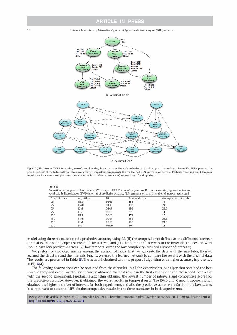
Fig. 8. (a) The learned TNBN for a subsystem of a combined cycle power plant. For each node the obtained temporal intervals are shown. The TNBN presents the

possible effects of the failure of two valves over different important components. (b) The learned DBN for the same domain. Dashed arrows represent temporal

transitions. Persistence arcs (between the same variable in different time slices) are not shown for simplicity.

Table 15

Evaluation on the power plant domain. We compare LIPS, Friedman’s algorithm, K-means clustering approximation and

equal-width discretization (EWD) in terms of predictive accuracy (BS), temporal error and number of intervals generated.

Num. of cases Algorithm BS Temporal error Average num. intervals

75 LIPS 0.063 18.1 16

75 EWD 0.131 19.5 24.5

75 K-M 0.143 19.3 24.5

75 F-G 0.065 27.5 14

150 LIPS 0.067 17.9 17

150 EWD 0.081 18.5 24.5

150 K-M 0.096 18.9 24.5

150 F-G 0.066 26.7 14

model using three measures: (i) the predictive accuracy using BS, (ii) the temporal error defined as the difference betweenthe real event and the expected mean of the interval, and (iii) the number of intervals in the network. The best networkshould have low predictive error (BS), low temporal error and low complexity (reduced number of intervals).

We performed two experiments varying the number of cases. First, we generate the data with the simulator, then welearned the structure and the intervals. Finally, we used the learned network to compare the results with the original data.The results are presented in Table 15. The network obtained with the proposed algorithmwith higher accuracy is presentedin Fig. 8(a).

The following observations can be obtained from these results. In all the experiments, our algorithm obtained the bestscore in temporal error. For the Brier score, it obtained the best result in the first experiment and the second best resultwith the second experiment. Friedman’s algorithm obtained the lowest number of intervals and competitive scores forthe predictive accuracy. However, it obtained the worst results in temporal error. The EWD and K-means approximationobtained the highest number of intervals for both experiments and also the predictive scores were far from the best scores.It is important to note that LIPS obtains competitive results in the three measures in both experiments.




7.3. Comparison with DBNs

For comparison purposes, we used the complete data (150 instances) from the simulator to learn a dynamic Bayesiannetwork. DBNs are similar to static BNs, in this case a probabilistic model is created to represent a process at a single point intime. Multiple copies of this model are then generated for each time point or slice belonging to a temporal range of interest.Links between copies are inserted to capture temporal relations.

Learning a DBN can be seen as a two stage process. The first stage refers to the learning of the static model and is done inan identical manner as we dowith classic BNs. The second stage learns the transition network, that is, the temporal relationsbetween randomvariables of different time slices. For this experimentwe learned a simpleDBNusing the sameK2 algorithmused in the TNBN to generate the static network. The transition network was learned using the Kevin Murphy’s Bayesiannetwork toolbox [16] with the Bayesian information criterion to select the best parents from the previous time slice.

Fig. 8(b) shows the learned DBN as a 2-time-slice BN, solid arrows represent arcs in the same time step, dashed arrowsrepresent temporal transition arcs. In particular, persistence arcs (between the same variable but in consecutive time steps)were omitted for readability. The learned DBN shows some common relations with the TNBN. A total of 10 temporal arcswere learned by the DBN and 9 arcs by the TNBNs, 5 of them were learned by both models. In particular the path: failure( failure steam valve ( electrical generation disturbance ( steam flow disturbance is present in the TNBN and the DBN. Incontrast, in the TNBN the path failure( failurewater valve( feedwater flowdisturbance( drum level disturbance is present,however in the DBN, the path is not complete, missing the arc between failure water valve ( feedwater flow disturbance.However, the DBN was able to learn an arc between drum pressure and drum level, nodes which are indeed related, but indid not appear in the TNBN.

This example shows how TNBNs can be simpler in some domains providing an easier to understandmodel in cases whena series of temporal events could occur. In the case of the DBNs these series of events are harder to see because of the waythe model is learned and represented. Also, it is important to notice that DBNs only represent the current time step and thenext one (the interval size is fixed), in contrast the TNBN represents a number of different intervals of different size. If wewanted to capture all the intervals of the TNBN we would need to repeat the structure many times producing a clutteredDBN.

8. Conclusions and future research

We developed a method for learning both, the structure and the temporal intervals for a TNBN from data. The algorithmperforms threesteps: thefirstoneobtainsabasic approximation to the intervalsusinganequalwidthdiscretizationalgorithmor an approximation based on k-means clustering. The second step obtains a structure of the TNBN using the intervalsobtained in the first step. The algorithm to obtain the structure is the one presented in [3]. The third step performs aninterval learning algorithm using the structure obtained in the previous step. For this, it initially generates a set of candidateintervals for each Temporal Node based on a Gaussian clustering algorithm. Then, the best intervals are selected based ontheir predictive accuracy.We evaluated ourmethodwith synthetic data and compared it with the algorithm presented in [9]and two baseline algorithms. In general, both methods obtain similar results in terms of structure and predictive accuracy.However, our algorithm is better in balancing the temporal error and the predictive score, it is also more efficient in termsof temporal complexity.

As future research we propose different ideas. On one side, we have performed some preliminary experiments aboutthe iteration of interval learning and structural learning. In our results the algorithm obtained the same structure in smallnumber of iterations indicating some kind of convergence. However, we would like to formalize under what circumstancesconvergence is guaranteed. On the other side, we would like to apply our algorithm in a medical application regarding howHIV drugs affect the appearance of resistance mutations.

Acknowledgments

This work was partly supported by the European Union and the National Council of Science and Technology of Mexico(CONACyT) under the project FONCICYT 95185, Pablo Hernandez-Leal was supported by a scholarship from CONACyT, Grant234507. We thank Lindsey Fiedler-Cameras for providing the results of the dynamic Bayesian network.

References

[1] G. Arroyo-Figueroa, L.E. Sucar, A temporal Bayesian network for diagnosis and prediction, in: Proceedings of the 15th UAI Conference. Stockholm, Sweden,1999, pp. 13–22.

[2] G. Brier, Verification of forecasts expressed in terms of probability, Monthly Weather Review 78 (1) (1950) 1–3.[3] G. Cooper, E. Herskovits, A Bayesian method for the induction of probabilistic networks from data, Machine Learning 9 (4) (1992) 309–347.[4] P. Dagum, A. Galper, E. Horvitz, Dynamic network models for forecasting, in: Proceedings of the 8th Workshop UAI, Stanford, California, USA, 1992, pp.

41–48.[5] T. Dean, K. Kanazawa, A model for reasoning about persistence and causation, Computational Intelligence 5 (2) (1989) 142–150.




[6] A.P. Dempster, N.M. Laird, D.B. Rubin, Maximum likelihood from incomplete data via the EM algorithm, Journal of the Royal Statistical Society 39 (1) (1977)1–38.

[7] I. Dogan, Analysis of facility location model using Bayesian networks, Expert Systems with Applications 39 (1) (2012) 1092–1104.[8] R. Duda, P. Hart, D. Stork, Pattern classification, vol. 2, wiley, New York, 2001.[9] N. Friedman, M. Goldszmidt, Discretizing continuous attributes while learning Bayesian networks, in: Machine Learning, Proceedings of the Thirteenth

International Conference (ICML’96), Bari, Italy, 1996, pp. 157–165.[10] S. Galán, G. Arroyo-Figueroa, F. Díez, L. Sucar, Comparison of two types of event Bayesian networks: A case study, Applied Artificial Intelligence 21 (3)

(2007) 185..[11] P. Hernandez-Leal, L. Sucar, J. Gonzalez, Learning temporal nodes Bayesian networks, in: The 24th Florida Artificial Intelligence Research Society Conference

(FLAIRS-24), Palm Beach, Florida, USA, 2011.[12] P. Kisioglu, Y.I. Topcu, Applying Bayesian belief network approach to customer churn analysis: a case study on the telecom industry of turkey, Expert

Systems with Applications 38 (6) (2011) 7151–7157.[13] W. Kruskal, W. Wallis, Use of ranks in one-criterion variance analysis, Journal of the American Statistical Association (1952) 583–621.[14] W. Lam, F. Bacchus, of Waterloo. Dept. of Computer Science, U., of Waterloo, Faculty of Mathematics, U., Learning Bayesian belief networks: an approach

based on the MDL principle, Computational intelligence, 10(4), 1994, pp. 269–293.[15] W. Liu, N. Song, H. Yao, Temporal functional dependencies and temporal nodes Bayesian networks, The Computer Journal 48 (1) (2005) 30–41.[16] K. Murphy, The Bayes net toolbox for matlab, Computing Science and Statistics 33 (2) (2001) 1024–1034.[17] R. Neapolitan, Learning Bayesian networks, Pearson Prentice Hall, Upper Saddle River, NJ, 2004.[18] J. Pearl, Probabilistic reasoning in intelligent systems: networks of plausible inference, Morgan Kaufmann Publishers Inc., San Francisco, CA, USA, 1988.[19] O. Pourret, P. Nam, P. Naïm, B. Marcot, Bayesian Networks: A Practical Guide to Applications, vol. 73, Wiley, 2008.[20] Y. Sun, Y. Tang, S. Ding, S. Lv, Y. Cui, Diagnose the mild cognitive impairment by constructing Bayesian network with missing data, Expert Systems with

Applications 38 (1) (2011) 442–449.[21] X. Wu, P. Lucas, S. Kerr, R. Dijkhuizen, Learning Bayesian-network topologies in realistic medical domains, Medical Data Analysis (2001) 302–307.



learning temporal nodes bayesian networks - inaoeemorales/papers/2013/2013... · learning temporal...

Documents