Learning robustly stable open-loop motions for roboticmanipulation

Wouter Wolfslag1,2,∗, Michiel Plooij1,2, Robert Babuska and Martijn Wisse2

Delft University of Technology1 These authors contributed equally to this work

2 These authors have received funding from the research programme STW, which is (partly)financed by the Netherlands Organisation for Scientific Research (NWO).

* Corresponding authorDelft University of Technology

Mekelweg 22628 CD Delft

The Netherlandsw.j.wolfslag@tudelft.nl

Abstract

Robotic arms have been shown to be able to perform cyclic tasks with an open-

loop stable controller. However, model errors make it hard to predict in simula-

tion what cycle the real arm will perform. This makes it difficult to accurately

perform pick and place tasks using an open-loop stable controller. This paper

presents an approach to make open-loop controllers follow the desired cycles

more accurately. First, we check if the desired cycle is robustly open-loop sta-

ble, meaning that it is stable even when the model is not accurate. A novel

robustness test using linear matrix inequalities is introduced for this purpose.

Second, using repetitive control we learn the open loop controller that tracks

the desired cycle. Hardware experiments show that using this method, the ac-

curacy of the task execution is improved to a precision of 2.5cm, which suffices

for many pick and place tasks.

Keywords: Feedforward control, open-loop control, robotic arms, robustness,

linear matrix inequalities, repetitive control

Preprint submitted to Elsevier November 26, 2014

1. Introduction

This research aims at future applications where sensing and feedback are

undesirable due to costs or weight; or difficult due to small scale, radiation

in the environment or frequent sensor faults. A recent example of such an

application is the control of a swarm of nano-scale medical robots [1]. These

applications inspire us to investigate an extreme case of feedback limitations:

solely open-loop control on robotic arms. Control without any feedback can

only be effective if two key problems are addressed: disturbances (e.g. noise

and perturbations) and model inaccuracies.

The first problem, handling disturbances on an open-loop controlled robot,

has mainly been addressed by creating open-loop stable cycles. The best known

examples of this are passive dynamic walkers, as introduced by McGeer in 1990

[2]. Since those walkers do not have any actuators, there is no computer feedback

control. The walking cycle of those walkers is stable, which means that small

perturbations will decay over time. Such stable cyclic motions are called limit

cycles. Limit cycle theory was later used to perform stable walking motions with

active walkers, of which the closest related work is that by Mombaur et al. [3, 4].

They optimized open-loop controllers for both stability and energy consumption

and performed stable walking and running motions with those robots. Open-

loop stable motions have also been used before to perform tasks with robotic

arms. In 1993, Schaal and Atkeson showed open loop stable juggling with a

robotic arm [5]. Even though their controller had no information about the

position of the ball, they showed that any perturbation in this position decays

over time, as long as a specific path of the robotic arm itself can be tracked. In

a recent study, we showed that it is possible to perform repetitive tasks on a

robotic arm with solely an open-loop current controller [6].

The second key problem with feedforward control (i.e. model inaccuracies)

prevents the approach in [6] to be fully applicable: it causes a difference between

the motion as planned in simulation and as performed in hardware experiments.

Handling model inaccuracies on open-loop controlled robots has recently be-

2

Pick position

Place position

Robust open loop stable cycle

Repetitive control

T2

T1

θ1

θ2

ω1

ω2

Learned open loop controller

Delayed removable feedback

Figure 1: This figure shows the top view of the concept of robust open-loop stable manipula-

tion. We first optimize a cycle that stands still at the pick and place positions for open-loop

stability. Next, we check the cycle for robustness to model uncertainty. Then, using repetitive

control on the robotic arm, we learn an open-loop controller that tracks the cycle. After the

learning, the open-loop controller performs the task without any feedback.

come the subject of research. Singhose, Seering and Singer [7, 8] researched

vibration reducing input shaping of open-loop controllers while being robust to

uncertainty in the natural frequency and damping of the system. Becker and

Bretl [9] researched the effect of an inaccurate wheel diameter of unicycles on

the performance of their open-loop velocity controller. In their case, open-loop

control means that the position of the unicycle is not used as an input for the

controller, but the velocity of the wheels is. In a previous paper, we showed

that on a robotic arm, different open-loop current controllers have different sen-

sitivities to model inaccuracies [10]. We found open-loop current controllers of

which the end position of the motion is independent of the friction parameters.

3

However, the motions that handle the model inaccuracy problem of feedfor-

ward control, the stability problem still exists, i.e., disturbances acting on these

motions will grow over time.

Since these two problems of disturbances and model inaccuracies in open-

loop control have only been addressed separately, no applicable purely open-loop

control scheme has been devised. This paper shows that repetitive tasks can

be performed stably by robotic arms with an open-loop voltage controller, even

when an accurate model is not available.

In order to achieve this goal, the problem is split into two phases (see Fig. 1).

In the first phase the robustness of the system is analyzed with a novel method

based on linear matrix inequalities (LMI)[11]. In the second phase repetitive

control (RC)[12] is used to learn the exact control input, such that the desired

positions are reached accurately. During this learning phase, very slow feedback

is allowed, this feedback can be removed after the learning has been completed.

The rest of this paper is structured as follows. Section 2 shows why the prob-

lem can be split into two phases, and explains the robustness analysis method

and the repetitive control scheme. Next, Section 3 shows the experimental setup

we used to test our approach. Then, Section 4 shows the results of both the nu-

merical and the hardware experiments. Finally, the paper ends with a discussion

in Section 5 and a conclusion in Section 6.

2. Methods

In this section we explain our methods. First, in Section 2.1 we discuss the

basic concept of the stability analysis. Second, Section 2.2 explains our approach

to perform robustly stable open-loop cycles. Then we will describe the two steps

of this approach separately: a robust stability analysis (Section 2.3) and learning

of an open-loop controller (Section 2.4).

2.1. Open-loop stable manipulation

A system described by the differential equation x = f(x, u) can be linearized

along a trajectory x∗ caused by input u∗(t):

4

dx

dt= A∗(t)x (1)

with

A∗(t) =∂f

∂x

∣∣∣∣x∗(t),u∗(t)

(2)

where x(t) = x(t) − x(t)∗ is the state error. For the ease of notation, the

time dependency of variables is occasionally dropped if it is unambiguous to do

so. For example A∗(t) will be written as A∗.

If both trajectory and input are cyclic with period tf , stability can be as-

sessed by by discretizing the system using a time step tf . To be able to draw

upon the research in stability of limit cycles, note that such discretization is

the same as a Poincare map of the system with the time appended to the state

vector. The Poincare section is then taken as t = tf , and the time is reset

to 0 after crossing this section. Previously (notably in [3] and [6]), verifying

stability was done using the eigenvalues of the linearized discrete system. But

that approach does not allow incorporating model uncertainty in the stability

analysis.

To obtain a method that does allow uncertain models, we use a quadratic

Lyapunov function, J = xTM(t)x, with positive definite M(t). The idea is

that for a stable system, an M(t) can be found such that the norm J is always

decreasing over time. For cyclic systems this means the following two constraints

should be satisfied (cf. [13]):

M(t)A(t)∗ + M(t) +A(t)∗T

M(t) ≺ 0, ∀t ∈ [t0, tf ] C1

M(tf )−M(t0) � 0 C2

where ≺ and � are used to indicate negative/positive definiteness respec-

tively, M is the time derivative of M and the subscripts 0 and f denote ini-

tial/final time. The first of these constraints ensures that the Lyapunov function

is decreasing at each time instant. The second constraint makes sure that it be-

comes stricter after each cycle, i.e., that having the same error (x) as a cycle

5

before means that the Lyapunov function has increased. Note that only one of

the two inequalities needs to be strict in order for stability to hold.

When there are model inaccuracies, two changes occur that make the above

conditions invalid. Firstly, A∗(x∗(t)) is no longer accurate when in state x∗(t).

Secondly, when using a fixed open-loop controller on an uncertain system, the

trajectory is not fully predictable, so in general x(t) 6= x∗(t), when using the

input u∗(t). In the next section we will outline our approach to solve these two

issues.

2.2. Robust open-loop approach

To find motions that are open-loop stable even when the model is not accu-

rately known, we will focus on input affine systems with constant input matrix,

i.e., systems that are described by the following differential equation:

x(t) = f(x(t)) +Bu(t) (3)

where B is a constant matrix. The equations of motion of serial chain robots

can be written in this form, by considering phase-space rather than state space

(i.e. using momenta rather than velocities). Systems where the control input

enters the system via a constant matrix have the advantage that the linearized

error dynamics do not depend on u (cf. Eq. (2)):

A∗(t) =∂f

∂x

∣∣∣∣x∗(t)

(4)

Because the local stability of the motion only depends on the linearized error

dynamics, the stability for motions of such a system only depends on the states

of the motion, and not on the inputs used. This is the key insight that allows

robust open-loop control, by splitting the problem into two stages:

1. Finding a trajectory through the phase-space that is stable, even if the

(linearized) system dynamics differ from their nominal value by some un-

certain amount.

6

2. Learning the inputs for that trajectory. When done online, this learning

can take into account the uncertain dynamics.

With this two stage approach, an open-loop controller is found that accu-

rately controls the robot in a way that is both accurate and stable. These

two properties hold even when facing modeling errors, which is important for

hardware implementation.

There are two important remarks to be made about this approach. Firstly,

the robust trajectory found should be a valid trajectory for the physical sys-

tem, and thus for all realizations of the uncertainty in the model. That means

there should exist an input for which the trajectory given is a solution to the

differential equation. In our case this means the inertia matrix has to be known

accurately in order to translate momenta into the velocities that correspond to

the time derivatives of the positions in the planned trajectories. Secondly, for

the learning step some feedback is required, which means the robot is no longer

purely open-loop controlled. However, such feedback can be delayed and can

be removed once the feedforward signal is known. This allows opportunities for

external sensing, such as cameras based feedback during the learning phase.

In Section 2.3 the methods used to find a robust trajectory will be explained.

Section 2.4 explains how Repetitive Control is used to learn the open-loop con-

troller.

2.3. Finding robustly stable trajectories

The first step in our approach is to find trajectories that are stable. To do

so, we use an optimization approach, further explained in Section 3. Then we

test if the resulting trajectory is robustly stable. In this section we derive a

novel robustness test, which is summarized in Algorithm 1.

For this section, we assume that we have a known trajectory for which we

want to determine how robust it is. We model the uncertainty of the system

through an integer number of uncertain parameters δj , that enter the lineariza-

tion affinely using known state and time dependent matrices ∆j(t), i.e.

7

A(t) =∂f

∂x

∣∣∣∣x=x∗(t)

+∑j

∆j(t)δj (5)

where we will take A∗(t) =∂f

∂x

∣∣∣∣x∗(t)

as the certain part of the dynamics,

and ∆(t) =∑j

∆j(t)δj as the uncertain part. Here the ∆j are known matrices

describing how the uncertain parameters δj enter the system dynamics. As a

result, we have a time varying uncertain system ˙x = A(t,∆)x = (A∗(t)+∆(t))x.

From theory of Linear Matrix Inequalities [11, Prop. 5.3], we know that if

each δj is constrained to some interval δj ∈ [δj , δj ], then the constraint C1 holds

for all ∆(t), if it holds for the ∆(t) created by the vertices of the hypercube of

allowed δj . The ∆(t) values connected to these vertices will be called ∆0(t),

which is a finite set. The choice for ∆0(t) depends on the expected model

inaccuracies. The robust stability constraint now becomes:

MA∗ + M +A∗TM + ∆T0M +M∆0 ≺ 0 C3

Note that this constraint is a sufficient, but not necessary condition for robust

stability. Making M a function of ∆ would reduce the conservativeness [11].

However, in implementation this would also result in much greater complexity

and computation time, so we have elected not to do so.

Furthermore, constraint C3 determines whether the trajectory is robustly

stable or not, but it does not give a continuous measure of robustness. To add

this measure, we try to find the maximal constant εx, such that the following

constraint holds:

MA∗ + M +A∗TM + εx∆T0M + εxM∆0 ≺ 0 C4

The value of εx is the robustness measure.

What is left is a way to find an M(t) that satisfies the constraints. Before

describing our approach, we will briefly discuss two approaches that involve

optimizing a parametrized M(t), and are unsuitable in this case, but at first

sight might seem applicable.

8

The first of these approaches is the most straightforward conceptually and

has been used in literature [13, 14, 15]. The idea in that research is to parametrize

M(t), and then optimize these parameters. The literature referred to establishes

that this parameter optimization can be cast as a convex problem by using Sum

Of Squares programming. The disadvantage of this approach for our problem

is that the optimization of M(t) requires many (> 1000) decision variables and

is therefore computationally expensive and sensitive to numerical errors.

The second approach is to parametrize M(0) only, and rework equation C1

or C3 into a differential equation, which can be integrated to find M(t). The

basic example would be

M = −εsI −A∗T

M −MA∗ (6)

with εs a small positive constant. This allows to optimize M(0), such that M(tf )

found using integration satisfies equation C2. This approach of integrating M

could potentially be extended to incorporate the uncertain dynamics into the

differential equations, for instance by viewing M as an ellipsoid, and using a

minimum volume ellipsoid covering algorithm. However, even then the method

of searching for M(0) and using forward integration is troublesome. The number

of parameters is greatly reduced compared to approaches where M(t) as a whole

is approximated and optimized, but at the cost of loosing convexity. This greatly

increases the computation time and introduces the risk of finding local minima.

Since these two approaches that involve searching for M(t) do not work, we

propose a method which does not involve such optimization, but rather immedi-

ately computes a (suboptimal) M(t). This method is based on the fact that all

time varying systems with periodic coefficients are reducible [16, Sec. XIV.3], i.e.

can be transformed into a time invariant system. The idea is to find a Lyapunov

function for the certain part of this time invariant system and then transform

this Lyapunov function back to the time variant system for the robustness check.

The transformation to the time invariant system is based on the state tran-

sition matrix of the nominal system x(t) = Φ(t)x(0), which can be found by

9

integrating the following initial value problem:

Φ(t) = A∗(t)Φ(t), Φ(0) = I (7)

Now if we define L(t) = Φ(t)Φ(tf )− t

tf and the transformation x = L(t)y, we

get for the state transition matrix of y:

y =1

tfln(Φ(tf ))y (8)

which is a time invariant, but possibly complex-valued system [16, Sec. XIV.1].

For this system we can then find a Lyapunov function yTMyy by solving for

the positive definite matrix My using standard LMI techniques. In principle it

would be possible to incorporate a worst-case transformed ∆(t) in that equation,

but for simplicity we optimize to find a Lyapunov function with the smallest

time derivative, i.e. maximize εy in:

1

tfln(Φ(tf ))TMy +My

1

tfln(Φ(tf )) + εyI ≺ 0 (9)

The resulting My is then transformed back to x coordinates:

M(t) = L(t)−TMyL(t)−1 (10)

Finally, the maximum εx that satisfies constraint C4 at all times is found

using a numerical LMI solver. The time derivative of M that is needed for this

step is readily determined analytically. We omit these expressions because they

are too lenghty.

As Eq. (7) can only be solved numerically, a natural time sampling approach

is used. That is, the constraint C4 is only tested at the sampling times that

are used by the solver that integrates Eq (7). In this case, we used the MAT-

LAB ode45 solver. This time sampling is inspired by [13], which discusses the

correctness of such a sampling procedure for a similar robustness test.

In many cases one or more of the singular values of the state transition

matrix Φ(tf ) are nearly zero [17]. This means that some errors are reduced to

nearly zero after one cycle. This can happen for instance with a high damping

constant, which could arise from using voltage control.

10

Space of nonsingular solutions

Basis for solution space

Nearly singular direction

t = 0 or t = tf t ≠ 0 and t ≠ tf

Basis for nonsingular solution space

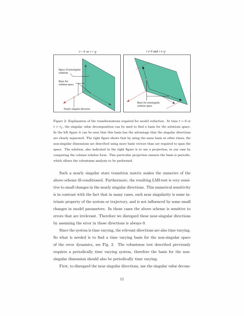
Figure 2: Explanation of the transformations required for model reduction. At time t = 0 or

t = tf , the singular value decomposition can be used to find a basis for the solutions space.

In the left figure it can be seen that this basis has the advantage that the singular directions

are clearly separated. The right figure shows that by using the same basis at other times, the

non-singular dimensions are described using more basis vectors than are required to span the

space. The solution, also indicated in the right figure is to use a projection, in our case by

computing the column echelon form. This particular projection ensures the basis is periodic,

which allows the robustness analysis to be performed.

Such a nearly singular state transition matrix makes the numerics of the

above scheme ill-conditioned. Furthermore, the resulting LMI-test is very sensi-

tive to small changes in the nearly singular directions. This numerical sensitivity

is in contrast with the fact that in many cases, such near singularity is some in-

trinsic property of the system or trajectory, and is not influenced by some small

changes in model parameters. In those cases the above scheme is sensitive to

errors that are irrelevant. Therefore we disregard these near-singular directions

by assuming the error in those directions is always 0.

Since the system is time varying, the relevant directions are also time varying.

So what is needed is to find a time varying basis for the non-singular space

of the error dynamics, see Fig. 2. The robustness test described previously

requires a periodically time varying system, therefore the basis for the non-

singular dimension should also be periodically time varying.

First, to disregard the near singular directions, use the singular value decom-

11

position of the state transition matrix at time tf : Φ(tf ) = UΣV T . Define Uχ

as the columns of U that correspond to the singular values that are not nearly

0. These columns are an orthonormal basis for the not-nearly-singular space

of Φ(tf ). In particular, define x(t) coordinates by the transformation x = Ux.

Then

Φ(t) = U−1Φ(t)[Uχ, 0] (11)

is the state transition matrix for x, where the errors in the singular di-

mensions are immediately set to zero (by the multiplication with [Uχ, 0]). The

columns of U Φ(t) now form a time varying basis for the non-singular space of

the x-dynamics. However, this basis is not periodic yet.

This periodicity can be enforced by using the following transformation, which

defines x(t):

x(t) = Urcef(

Φ(t))x(t) (12)

where rcef signifies the reduced column echelon form. To see that it works,

it is necessary to realize that after exactly one cycle, the columns of Φ span

the same space. Furthermore, Φ(0) is simply the identity matrix with the last

diagonal entries turned into 0. Therefore Φ(tf ) also spans this same space,

and the reduced column echelon form then finds the correct basis: the identity

matrix with the last entries turned into 0. As a result rcef(Φ(0)) = rcef(Φ(tf )).

This means that the transformation in Eq. 12 is periodic, and can therefore be

used in the robustness test. The procedure of the robustness test, including this

transformation is denoted in Algorithm 1, in which each step is described and

the relevant equations for that step are then referred to.

This leaves only two remarks on the implementation of this transformation.

First, the reduced column echelon form of a smoothly varying matrix is smoothly

varying, meaning the time derivative of the transformation exists. To speed up

computation we use finite differences to compute this derivative. Second,the

transformation as defined above does not actually reduce the number of states

in the computation, but rather sets the states to zero. By substituting Uχ for

[Uχ, 0] in Eq. 11, the size of the state vector is reduced, which again speeds up

12

computation.

Algorithm 1 Robustness test

Compute state transition matrix Φ(tf ), Eq. (7)

if nearlySingular(Φ(tf )) then

Reduce system dimension, Eqs. (11)-(12)

end if

Make system time invariant by transformation, Eq. (8)

Find My, the Lyapunov function for that system, Eq. (9)

Initialize robustness measure, εx ← 1000

for all t in time discretization do

Find M(t), Lyapunov function of first system, Eq. (10)

Numerically find M(t) as required in constraint C4.

ε← maximum εx that satisfies constraint C4 at time t

εx ← min(ε,εx)

end for

2.4. Repetitive control

The stability of the trajectories computed by the optimization is independent

of the input and finite modeling errors. The next step is to learn the input that

tracks the trajectory on the robotic arm. When the trajectory is learned, the

feedback is disconnected and the task is performed stably with the learned

open-loop controller.

There are two (similar) learning algorithms which are commonly used for

learning of repetitive motions: Iterative Learning Control (ILC) and Repetitive

Control (RC) [12]. Both algorithms use the input and error from the previous

iteration (cycle) to compute the input in the current iteration. The only dif-

ference between the two is that in ILC every iteration starts at the same state,

where in RC every iteration starts at the final state of the previous iteration.

We use RC, because it allows us to immediately start a new iteration at the end

of every movement cycle, whereas ILC would require a reinitialization after ev-

13

ery cycle to start the new iteration, which would take time and require fast and

precise state feedback. The repetitive control runs on a real time target with

a sampling frequency of 500 Hz. Therefore, we will use discrete time notation

with time step k.

The repetitive control scheme we used is

u(k) = u(k − p) + α(k) · (∆uP (k) + ∆uD(k)) (13)

with

∆uP (k) =

p−1∑i=0

φ(i) · P · e(k − p+ i) (14)

∆uD(k) =

p−1∑i=0

σ(i) ·D · (e(k − p+ i)− x(k − 2p+ i)) (15)

x(k) = x∗(k)− x(k) (16)

where u(k) is the control input, p is the number of time steps in one iteration,

x(k) is the error, x∗ is the desired state and x is the actual state. α(k), φ(i),

σ(i), P and D are explained below.

The learning rate α(k) is a function of time and can vary between 0 and 1.

A varying α(k) reduces the chance of converging to a sub-optimal solution.

The filter gains φ(i) and σ(i), for i = 1, . . . , p, determine how much the

different errors in the previous iterations contribute to the change in the input

signal. The filtering accounts for measurement noise and prevents oscillations

in the RC. The sum of the elements of φ(i) and the sum of the elements of σ(i)

are both equal to 1, to obtain a (weighted) moving average filter.

The learning gains P and D are Nu ×Ns matrices (with Nu the number of

inputs and Ns the number of states). The P and D we used have the following

structures:

P =

P11 0 P13 0

0 P22 0 P24

(17)

D =

D11 0 D13 0

0 D22 0 D24

(18)

14

Using this structure, errors in the state of one joint have no direct influence on

the control signal in another joint (i.e. there are no cross terms). The ∆uP

term can be seen as the proportional term of the RC, since it leads to a change

in u proportional to the errors in the previous iteration. The ∆uD term can be

seen as the damping term of the RC between two iterations, since it leads to a

change in u proportional to the change in errors between two iterations.

3. Experimental setup

We tested our approach on a two DOF SCARA type arm. This type of arm

can perform industrially relevant tasks with a simple mechanical design. In the

experiment, the arm has to perform a rest to rest motion, typical for a pick

and place task. In this section the hardware setup and task description will be

addressed, along with parameters in our approach that were set specifically for

the experiments. Note however that the general approach does not depend on

the exact values of the parameters, which were manually tuned.

3.1. Hardware setup

Fig. 1 shows a picture of the experimental two DOF robotic arm [18]. The

arm consists of two 18x1.5mm stainless steel tubes, connected with two revolute

joints, with a spring on the first joint. A gripper is connected to the end of the

second tube. The motors are placed on a housing and AT3-gen III 16mm timing

belts are used to transfer torques within the housing. The joints are actuated

by Maxon 60W RE30 motors with gearbox ratios of respectively 66:1 and 18:1.

The timing belts provide additional transfer ratios of 5:4 on both joints. The

parameters of this robotic arm are listed in Table 1.

The large damping terms are caused by the back-emf of the motors (since

we use voltage control and not current control). The viscous and Coulomb

friction are neglected in this paper since they are small compared to the back-emf

induced damping. The equations of motion and the transformation to momenta

can be derived using standard methods [19, Chap. 3], and are ommitted from

15

Table 1: The model parameters of the two DOF arm.

Parameter Symbol Value Unit

Damping µv1, µv2 7.48, 0.56 Nms/rad

Inertia J1, J2 0.0233, 0.0871 kgm2

Mass m1, m2 0.809, 1.599 kg

Length l1, l2 0.410, 0.450 m

Position of COM lg1, lg2 0.070, 0.325 m

Motor constant kt1, kt2 25.9, 25.9 mNm/A

Gearbox ratio g1, g2 82.5:1, 22.5:1 rad/rad

Spring stiffness k1 1.6 Nm/rad

this paper because they are too long. Because the second joint is connected to

its motor via a parallelogram mechanism (see [18]), the angle of the second arm

is taken as the absolute angle, i.e., relative to the world frame.

3.2. Task description

We let the manipulator perform a cyclic pick and place motion, with pick

and place positions at [0.4, 0.1] rad and [-0.2, -1.2] rad respectively. At the pick

and place position, the arm has to stand still for 0.2s, which would be required

to pick or place an object. The time to move between the pick and the place

position is 1.4s. Hence, the total time of one cycle is 3.2s.

3.3. Optimization

To find a robustly stable trajectory an optimization is used. First, the tra-

jectory is optimized for fast convergence, by minimizing the maximal eigenvalue

modulus of the linearized Poincare map, see the stability measure in [6]. The

input was taken as a piecewise linear input, consisting of 20 pieces, with an ab-

solute maximum value of 5V. Then, the robustness of the resulting trajectory is

verified using the approach outlined in Section 2. The uncertain dynamics ∆(t)

consist of two uncertainties: uncertainty on the linearized stiffness on the first

16

and second joint. The bounds on these uncertainties are constant and taken as

±0.3 and ±1.0 Nm/rad respectively.

3.4. Repetitive control parameters

We let the robotic arm learn the cycle from simulation while t < tRCfinal.

During this learning period, the learning gain decreased linearly from α = 1 at

t = 0 s to α = 0 at t = tRCfinal s.

The filter gains we used are equal to

φ(i) = σ(i) =−(i− 1) ∗ (i− 50)

| − (i− 1) ∗ (i− 50)|∀i ≤ 50 (19)

φ(i) = σ(i) = 0 ∀i > 50 (20)

The result of using these filter gains is that the change in input signal depends

on errors in steps k − p to k − p + 50, see Eq. 13. Therefore the RC scheme

is non-causal. This filter has two purposes. First, taking a weighed average

over multiple measurements reduces the influence of sensor noise. Second, the

non-causality takes into account that the input relates to the acceleration, which

means it takes some time to have a measurable effect on the state, which consists

of the positions and the velocities.

The remaining parameters are shown in Table 2. All PD and filter gains

we used in the repetitive control algorithm are based on experience rather than

on extensive calculations. Also, note that in this paper we do not not prove

that the repetitive controller is stable. Experience on the robot shows that the

repetitive controller is stable as long as the gains Pij and Dij are not too high.

4. Results

This section presents the results from both the optimization in simulation

and hardware experiments. First, using the LMI based robustness analysis,

we optimize the trajectory for both stability and robustness. Second, we learn

the open-loop controller that tracks this trajectory. When the controller is

17

Table 2: The parameters used in optimization and RC

Symbol Value Symbol Value

tRCfinal 300 s

P11 1.5 V/rad D11 0 V/rad

P22 0.6 V/rad D22 0.4 V/rad

P13 0.3 Vs/rad D13 0 Vs/rad

P24 0.4 Vs/rad D24 0 Vs/rad

learned, the feedback is disconnected and the robotic arms can perform its task

with solely open-loop control. The video accompanying this paper shows the

hardware experiments.

4.1. Simulation results

The red dashed lines in Figs. 3a-d show the cycle obtained from optimization.

The cycle has a maximal eigenvalue modulus of 0.70 and a robustness value of

εx= 0.038. These results are interpreted in Section 5.2.

4.2. Hardware results

Fig. 5 shows the learning curve of the repetitive control. It shows two curves

that correspond to the absolute position error of the end effector at the pick

positions (blue line) and the place position (red dashed line). These errors were

calculated by taking the errors at the time in the cycle when picking and placing

are to take place. The learning phase takes about 40 cycles, which corresponds

to 128s. After the cycle is learned, the error at the pick position is approximately

1cm and the error at the place position is approximately 2.5cm. These errors are

small enough to perform many basic pick and place tasks, as found for instance

in the food and packaging industry. Furthermore, these errors are also within

the grasping-ranges of modern robotic grippers[20][21]

The blue solid lines in Figs. 3a-d show the cycle after it was learned on the

robotic arm. The graphs show that the cycle on the robotic arm is the same as

the one obtained from simulation.

18

300 304 308−0.8

−0.4

0

0.4

time (s)

Posi

tion

(rad

)

300 304 308−2

−1

0

1

2

3

time (s)

Vel

ocity

(rad

/s)

300 304 308−1.5

−1

−0.5

0

0.5

time (s)

Posi

tion

(rad

)

300 304 308−3−2−10123

time (s)

Vel

ocity

(rad

/s)

Robotic armDesired cycle(a) (b)

(c) (d)

Figure 3: The cycle of the robotic arm after learning. The red dashed line shows the desired

cycle that was obtained from simulation. The blue solid line shows the cycle of the robotic

arm after 300s of learning. (a) The position of the first joint, (b) the position of the second

joint, (c) the velocity of the first joint and (d) the velocity of the second joint.

Fig. 4 shows the motion of the gripper in workspace. The red dashed line

shows the cycle that was obtained from simulation and the blue solid line shows

the robotic arm that starts at a perturbed state and converges to the desired

cycle. Within two cycles, the arm follows the desired cycle.

5. Discussion

5.1. Applicability

The techniques presented in this paper make open-loop stable manipulation

applicable. Previous work showed that model uncertainties lead to a cycle that

19

−0.4 −0.2 0 0.2 0.4 0.6

0.3

0.4

0.5

0.6

0.7

0.8

0.9

1

1.1

1.2

x position (m)

y po

sitio

n (m

)

Robotic armDesired cycle

Figure 4: This figure shows the motion of the arm in workspace. The red dashed line shows the

desired cycle that was obtained from optimization. The blue solid line shows the motion of the

robotic arm that does not start on the cycle but converges to the cycle. After approximately

two cycles, the arm returns to tracking the desired cycle with its final accuracy of 2.5 cm.

differs too much from the intended cycle to be applicable in e.g. pick and place

tasks [6]. With the learning of the open-loop controller, the errors in the position

of the gripper decreased to 1-2.5cm. Furthermore, when the arm is perturbed,

it converges back to the desired cycle within approximately two cycles.

Some applications, however, might require a more accurate controller (i.e.

with errors smaller than 2.5 cm). There are no fundamental problems that limit

the accuracy of our approach. There are however, two problems specific to our

robotic arm and implementation that do limit the accuracy. Firstly, velocity

estimation is not accurate due to quantization noise due to a coarse encoder.

This makes it hard to learn the desired cycle. Secondly, the state is filtered

in our implementation of repetitive control, leading to a smooth control signal.

20

0 20 40 60 80 1000

0.1

0.2

0.3

0.4

0.5

0.6

0.7

0.8

0.9

Cycles

Erro

r (m

)

Pick positionPlace position

Figure 5: The abcolute error in the pick and place positions while learning. This graph shows

that the absolute error decreases to approximately 1 cm for the pick position and 2.5 cm for

the place position.

However, a non-smooth control signal might be required to track the desired

cycle more accurately. In conclusion, depending on the application, the setup

and implementation can be changed to increase the accuracy to the desired level.

The learned feedforward approach is applicable to many tasks. A new cyclic

task can be handled by the same procedure of learning a feedforward trajectory,

testing the robustness with Algorithm 1, and learning the input signal with

repetitive control. At the moment the learning takes the most time, 300s. The

optimization (1s) and robustness test (5s) take much less time. Reducing the

time needed to learn a new task will further increase the applicability and is

therefore an important part of our future research.

The main drawback of the current approach is that some feedback is required

during the learning phase. However, this feedback can be delayed (almost a

21

whole cycle) and can be removed after the learning has finished. The (delayed)

feedback could therefore be provided by e.g. cameras. One interesting direction

for future work would be to research repetitive control schemes without full state

feedback. This could mean omitting certain states or reducing the frequency of

the feedback.

This feedback requirement also comes up in situations where large distur-

bances are expected to occur after learning. In such situations the robot should

know whether it has converged back to the desired cycle. This requirement can

be satisfied with cameras, or even more basically, by using a switch at a certain

position that checks the timing of passing that position.

5.2. Interpreting robustness measure

The robustness test depends on the choice of ∆, which is to some degree

arbitrary. In previous experiments on this robotic arm, bending of the second

joint was hypothesized to be one of the main causes of model-reality mismatch

[6]. Therefore ∆ was chosen to emphasize this error, which depends only on the

position of the second joint.

For the chosen ∆, the resulting robustness measure εx of 0.038 indicates that

the spring stiffness of ±0.038 Nm/rad could be added to the second joint. This

seems insignificant to the effective spring stiffness of around 1.6 Nm/rad that

is in place on the first joint. However, note that adding any negative spring

stiffness to the second joint would make that joint unstable by itself. Therefore

low values of εx should be expected.

5.3. Hybrid systems and Coulomb Friction

Despite the fact that robustness against modeling errors is checked, there

are still two modeling-related issues that are not accounted for in the current

approach. Firstly, when performing an actual pick and place motion, the model

will consist of two phases with different end-point masses with an impact phase

in between to model the grasping. Secondly, a more accurate friction model

would include Coulomb friction. Both these effects can be added by using a

22

hybrid system model. Such hybrid models are quite generally used in analysis

of systems with limit cycles, mostly to cope with impact in walking, e.g. [22].

Under some basic transversality conditions, as discussed in [23], the current

approach can be extended to such hybrid models. We see that inclusion as the

logical next step in the research in open-loop control of robotic arms.

5.4. Scalability

The experiments were done on a two DOF robotic arm. Such an arm has

similar dynamics to SCARA type arms, which are often used in industry. The

current approach therefore already can be used for realistic industrial situations.

However, there are also many robotic arms which have a larger number of joints

and rotate in 3D. For such a setup the approach remains untested.

There are three possible concerns for this approach for higher DOF robots.

Firstly, there is the possibility that no stable trajectories exist. This is unlikely,

and it can be ensured not to happen if springs are used on all joints to stabilize

the system. Secondly, the required computation will become more extensive.

However, because only a feedforward signal is required, no full state exploration

is necessary. Furthermore, the number of free parameters in the robustness

approach is independent of the number of DOFs on the robot. Thirdly, although

earlier results on a two DOF arm suggest that the basin of attraction of our

approach is quite large [6], for multiple degrees of freedom it becomes more likely

that the robotic arm will converge to a different cycle after a large perturbation.

Again, this could be prevented by using springs on all joints to stabilize the

system. Combining all of the above, we expect that our approach scales well to

higher DOF robotic arms.

6. Conclusion

In this paper we showed that repetitive tasks can be performed stably by

robotic arms with an open-loop controller, even when an accurate model is not

available. We used an LMI-based robustness analysis to check the robustness

23

to model inaccuracies. We then used a repetitive control scheme to track this

trajectory with the robotic arm. Hardware experiments show that using this

approach, position errors can be reduced to 2.5 cm, making open-loop control

applicable in tasks such as picking and placing objects.

Acknowledgement

This work is part of the research programme STW, which is (partly) financed

by the Netherlands Organisation for Scientific Research (NWO).

[1] A. Becker, O. Felfoul, and P. E. Dupont, “Simultaneously powering and

controlling many actuators with a clinical mri scanner,” in Intelligent

Robots and Systems (IROS 2014), 2014 IEEE/RSJ International Confer-

ence on. IEEE, 2014, pp. 2017–2023.

[2] T. McGeer, “Passive dynamic walking,” The International Journal of

Robotics Research, vol. 9, no. 2, pp. 62–82, 1990.

[3] K. D. Mombaur, R. W. Longman, H. G. Bock, and J. P. Schloder,

“Open-loop stable running,” Robotica, vol. 23, no. 1, pp. 21–33, Jan. 2005.

[Online]. Available: http://dx.doi.org/10.1017/S026357470400058X

[4] K. D. Mombaur, H. G. Bock, J. P. Schloder, and R. W. Longman, “Open-

loop stable solutions of periodic optimal control problems in robotics,”

ZAMM-Journal of Applied Mathematics and Mechanics/Zeitschrift fur

Angewandte Mathematik und Mechanik, vol. 85, no. 7, pp. 499–515, 2005.

[5] S. Schaal and C. Atkeson, “Open loop stable control strategies for robot

juggling,” in Robotics and Automation, 1993. Proceedings., 1993 IEEE In-

ternational Conference on, may 1993, pp. 913 –918 vol.3.

[6] M. Plooij, W. Wolfslag, and M. Wisse, “Open loop stable control in

repetitive manipulation tasks,” in Robotics and Automation (ICRA), 2014

IEEE/RSJ International Conference on, may 2014.

24

[7] N. C. Singer and W. P. Seering, “Preshaping command inputs to reduce

system vibration,” Journal of Dynamic Systems, Measurement, and Con-

trol, vol. 112, pp. 76–82, 1990.

[8] W. Singhose, W. Seering, and N. Singer, “Residual vibration reduction

using vector diagrams to generate shaped inputs,” Journal of Mechanical

Design, vol. 116, pp. 654–659, 1994.

[9] A. Becker and T. Bretl, “Approximate steering of a unicycle under

bounded model perturbation using ensemble control,” IEEE Transactions

on Robotics, vol. 28, no. 3, pp. 580–591, 06 2012.

[10] M. Plooij, M. De Vries, W. Wolfslag, and M. Wisse, “Optimization of feed-

forward controllers to minimize sensitivity to model inaccuracies,” in In-

telligent Robots and Systems (IROS), 2013 IEEE/RSJ International Con-

ference on, nov. 2013.

[11] C. Scherer and S. Weiland, “Linear matrix inequalities in control,” Lecture

Notes, Dutch Institute for Systems and Control, Delft, The Netherlands,

2000.

[12] R. W. Longman, “Iterative learning control and repetitive control for en-

gineering practice,” International Journal of Control, vol. 73, no. 10, pp.

930–954, 2000.

[13] M. Tobenkin, I. Manchester, and R. Tedrake, “Invariant funnels around

trajectories using sum-of-squares programming,” in Proceedings of the 18th

IFAC World Congress, extended version available online: arXiv:1010.3013,

2011.

[14] A. Majumdar, “Robust online motion planning with reachable sets,” Ph.D.

dissertation, Massachusetts Institute of Technology, 2013.

[15] G. Chesi, Domain of Attraction: Analysis and Control via SOS Program-

ming. Springer, 2011.

25

[16] F. R. Gantmacher, The theory of matrices. Taylor & Francis US, 1960,

vol. 2.

[17] S. Revzen and J. Guckenheimer, “Finding the dimension of slow dynamics

in a rhythmic system,” Journal of The Royal Society Interface, vol. 9,

no. 70, pp. 957–971, 2012.

[18] M. Plooij and M. Wisse, “A novel spring mechanism to reduce energy

consumption of robotic arms,” in Intelligent Robots and Systems (IROS),

2012 IEEE/RSJ International Conference on, oct. 2012, pp. 2901 –2908.

[19] R. van der Linde and A. Schwab, “Lecture notes on multibody dynamics

b, wb1413,” Delft University of Technology, 1997/1998.

[20] E. Brown, N. Rodenberg, J. Amend, A. Mozeika, E. Steltz, M. R. Za-

kin, H. Lipson, and H. M. Jaeger, “Universal robotic gripper based on the

jamming of granular material,” Proceedings of the National Academy of

Sciences, vol. 107, no. 44, pp. 18 809–18 814, 2010.

[21] G. A. Kragten and J. L. Herder, “The ability of underactuated hands to

grasp and hold objects,” Mechanism and Machine Theory, vol. 45, no. 3,

pp. 408–425, 2010.

[22] E. Westervelt, J. Grizzle, and D. E. Koditschek, “Hybrid zero dynamics of

planar biped walkers,” Automatic Control, IEEE Transactions on, vol. 48,

no. 1, pp. 42–56, 2003.

[23] S. Burden, S. Revzen, and S. Sastry, “Dimension reduction near periodic

orbits of hybrid systems,” in Decision and Control and European Control

Conference (CDC-ECC), 2011 50th IEEE Conference on. IEEE, 2011,

pp. 6116–6121.

26