Learning Receptive Fields for Pooling from Tensors of Feature Response

Can Xu and Nuno VasconcelosDepartment of Electrical and Computer Engineering

University of California, San Diego{canxu, nuno}@ucsd.edu

Abstract

A new method for learning pooling receptive fields forrecognition is presented. The method exploits the statisticsof the 3D tensor of SIFT responses to an image. It is ar-gued that the eigentensors of this tensor contain the infor-mation necessary for learning class-specific pooling recep-tive fields. It is shown that this information can be extractedby a simple PCA analysis of a specific tensor flattening. Anovel algorithm is then proposed for fitting box-like recep-tive fields to the eigenimages extracted from a collection ofimages. The resulting receptive fields can be combined withany of the recently popular coding strategies for image clas-sification. This combination is experimentally shown to im-prove classification accuracy for both vector quantizationand Fisher vector (FV) encodings. It is then shown that thecombination of the FV encoding with the proposed recep-tive fields has state-of-the-art performance for both objectrecognition and scene classification. Finally, when com-pared with previous attempts at learning receptive fields forpooling, the method is simpler and achieves better results.

1. IntroductionObject recognition and scene classification are two im-

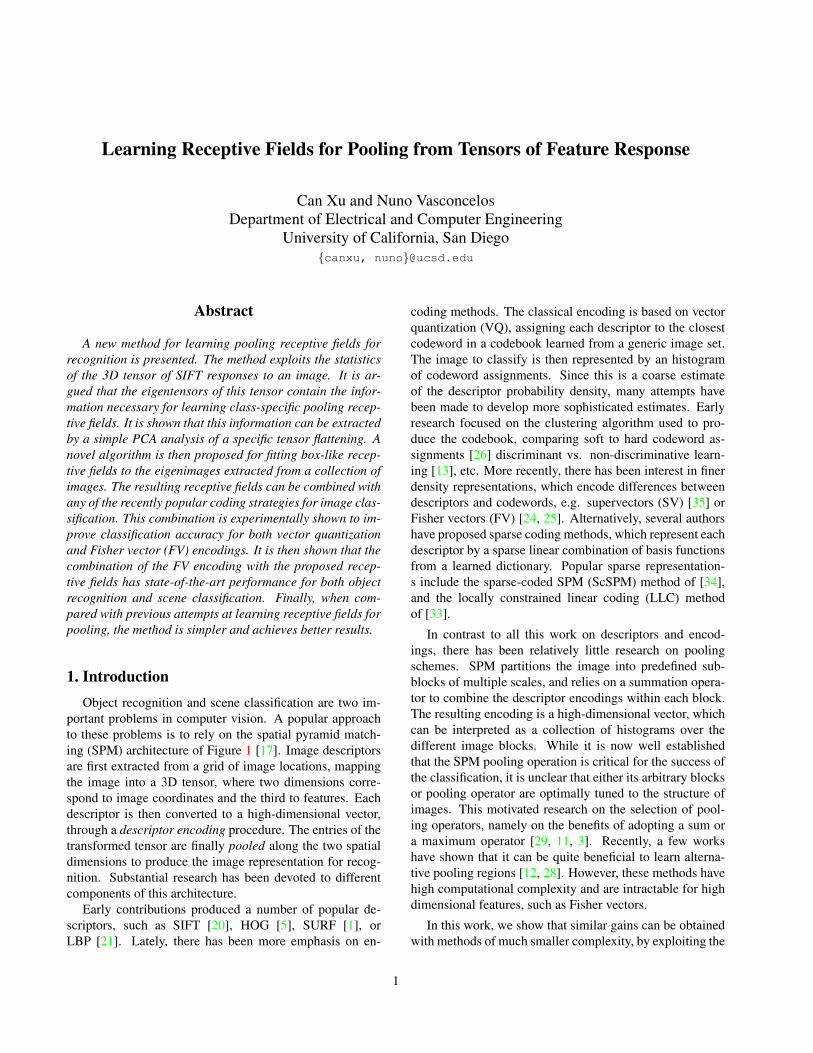
portant problems in computer vision. A popular approachto these problems is to rely on the spatial pyramid match-ing (SPM) architecture of Figure 1 [17]. Image descriptorsare first extracted from a grid of image locations, mappingthe image into a 3D tensor, where two dimensions corre-spond to image coordinates and the third to features. Eachdescriptor is then converted to a high-dimensional vector,through a descriptor encoding procedure. The entries of thetransformed tensor are finally pooled along the two spatialdimensions to produce the image representation for recog-nition. Substantial research has been devoted to differentcomponents of this architecture.

Early contributions produced a number of popular de-scriptors, such as SIFT [20], HOG [5], SURF [1], orLBP [21]. Lately, there has been more emphasis on en-

coding methods. The classical encoding is based on vectorquantization (VQ), assigning each descriptor to the closestcodeword in a codebook learned from a generic image set.The image to classify is then represented by an histogramof codeword assignments. Since this is a coarse estimateof the descriptor probability density, many attempts havebeen made to develop more sophisticated estimates. Earlyresearch focused on the clustering algorithm used to pro-duce the codebook, comparing soft to hard codeword as-signments [26] discriminant vs. non-discriminative learn-ing [13], etc. More recently, there has been interest in finerdensity representations, which encode differences betweendescriptors and codewords, e.g. supervectors (SV) [35] orFisher vectors (FV) [24, 25]. Alternatively, several authorshave proposed sparse coding methods, which represent eachdescriptor by a sparse linear combination of basis functionsfrom a learned dictionary. Popular sparse representation-s include the sparse-coded SPM (ScSPM) method of [34],and the locally constrained linear coding (LLC) methodof [33].

In contrast to all this work on descriptors and encod-ings, there has been relatively little research on poolingschemes. SPM partitions the image into predefined sub-blocks of multiple scales, and relies on a summation opera-tor to combine the descriptor encodings within each block.The resulting encoding is a high-dimensional vector, whichcan be interpreted as a collection of histograms over thedifferent image blocks. While it is now well establishedthat the SPM pooling operation is critical for the success ofthe classification, it is unclear that either its arbitrary blocksor pooling operator are optimally tuned to the structure ofimages. This motivated research on the selection of pool-ing operators, namely on the benefits of adopting a sum ora maximum operator [29, 11, 3]. Recently, a few workshave shown that it can be quite beneficial to learn alterna-tive pooling regions [12, 28]. However, these methods havehigh computational complexity and are intractable for highdimensional features, such as Fisher vectors.

In this work, we show that similar gains can be obtainedwith methods of much smaller complexity, by exploiting the

1

features

location

descriptor

codewords

coded descriptor feature tensor coding tensor

pooling

window

Figure 1: Under SPM, an image is first mapped into a tensor of feature (descriptor) responses and subsequently into a tensor of coding coefficients.Discriminant class information is coded as blobs of energy within these tensors. Discriminant pooling windows can be recovered by detecting the eigenblobsof tensor response to images of the class.

statistics of the 3D feature tensor of Figure 1. The hypoth-esis is that pooling regions can be learned by identifyingblobs of discriminant response, for each image class, in thetensor. We propose to identify these blobs as the locationswhere responses to images of the class have most energy.This equates pooling regions to eigentensors of the 3D ten-sor. One appealing property of this hypothesis is that thecomputation of eigentensors is computationally trivial. Itreduces to computing a principal component analysis (P-CA) of various 2D flattenings of the tensor [32, 31]. In fact,we show that a particular flattening corresponds to the pop-ular PCA-SIFT representation [14]. For learning to poolthis is the most uninteresting flattening, since it does notpreserve image topology.

We explore alternative flattenings, which preserve loca-tion information, and use them to identify potential poolingregions. We then introduce an algorithm for learning a set ofbox-like pooling regions that best approximates the eigen-tensors over a collection of images. This is a k-means likeprocedure, iterating between the assignment of eigentensorregions to boxes and the reshaping of boxes to fit regions. Itis a generic algorithm that could be applied to many visionproblems, e.g. determining an object bounding box from asaliency map or the output of an object detector [19]. Ex-perimental results show that the learned fields significantlyoutperform SPM and that the gains hold across encodings.We adopt the FV encoding and show that its combinationwith the proposed learned fields achieves state of the art re-sults on various datasets.

2. Learning receptive fields through tensors

We start by identifying candidate pooling regions fromthe statistics of the tensor of feature responses.

2.1. From image to tensor

Figure 1 illustrates how the SPM representation can bemapped into a tensor. Images are mapped into 128D SIFT

descriptors, which are stacked so as to maintain the imagetopology. In the resulting 3D tensor, each vector in thedirection orthogonal to the image coordinates correspond-s to a SIFT descriptor. The resulting structure is denotedthe feature tensor. SIFT descriptors are then mapped intohigh-dimensional codes. For example, into 1,024D vectorswhose entries are the assignments of a SIFT descriptor to acodebook of 1, 024 codewords. Again, these vectors are s-tacked to produce a tensor that respects the image topology.This is the coding tensor. SPM applies a set of pooling op-erators to this tensor, producing a feature vector that is fedto a support vector machine for classification. Pooling op-erators are sums over a preset pyramid of multi-scale imagewindows. The feature vector is an histogram of the code-word assignments in the associated image regions.

2.2. Learning to pool

While SPM relies on a sum operator and arbitrary pool-ing regions, some alternatives have been investigated in therecent literature. Most of this effort has been on improvedpooling operators. For example, Yang et al. [34] used maxinstead of sum pooling. Boureau and Ponce [3] later pro-vided a theoretical analysis, showing that max pooling iswell suited for features with a low probability of activation.However, other experiments have shown mixed results forthe benefits of the max over the sum operation [11]. Ourwork does not address the pooling operator, but the learn-ing of regions of support (windows) for pooling operators.These are denoted as the receptive fields for pooling.

The learning of receptive fields has been the subject ofattention in the last few years. Jia et al. [12] started froma large number of candidate rectangular boxes, and pro-posed a greedy method for learning the optimal receptivefields from this set. Russakovsky et al. [28] proposed anobject-centric spatial pooling approach, which jointly per-forms classification and localization through bootstrapping.These methods have demonstrated improved performanceon several benchmarks, but have substantial complexity and

Tensor

Eigen-tensors

Pooling

Fields

Figure 2: Receptive field learning. An image class defines an energy distribution in tensor space. An eigen-tensor decomposition produces the collection oftensor basis functions that best approximate this energy distribution. Discriminant pooling windows can be obtained from these eigentensors.

become intractable for high dimensional encodings, such asFisher vectors. For example, the method of [28] is too com-plex for standard SVM solvers, even when applied to a rel-atively low-dimensional VQ encoding. A slightly differentapproach was proposed by [15], which replace SPM with aspatial Fisher vector (SFV). This is a representation of thespatial distribution of SIFT descriptors.

In this work we seek a solution of much lower complex-ity, based on the intuition of Figure 2. Images are viewed asdistributions of energy in the feature tensor. The discrimi-nant visual structures of a given image class give rise to con-sistent energy blobs. Given a set of images from the class,these blobs can be approximated by a small set of tensoreigenfunctions, denoted eigen-tensors. The image location-s containing the bulk of the energy of the responses to theclass are then recovered from these eigen-tensors and usedas receptive fields for pooling.

2.3. Tensor Analysis

A tensor T ∈ Rk1×k2×...kN of order N is an ND ar-ray of k1 × k2 × . . . kN entries. In this work, we restrictour attention to tensors of order 3, whose coordinates cor-respond to image locations (k1), features (k2), and scales(k3). We rely on SIFT features, and different image scalesare obtained with a Gaussian pyramid [20]. A kn-D vec-tor obtained from T by varying index n while keeping theothers fixed is the mode-n vector of T . Mode-n vectors arethe column vectors of the matrix Tn ∈ Rkn×

∏i ̸=n ki that

results from flattening the tensor T with respect to dimen-sion n. Fig. 3 illustrates the three flattenings - T1,T2,T3

- of the 3rd order tensor. The N -mode singular value de-composition (SVD), is an extension of the matrix SVD thatexpresses the tensor as a product of N -orthogonal spaces

T = Z ×1 U1 . . .×N UN (1)

where A×n M is the n-mode product of a tensor A with amatrix M, defined as

B = A×n M ⇔ Bn = MAn. (2)

The mode matrix Un of (1) contains the orthonormal vec-tors spanning the column space of the mode-n flatteningmatrix Tn of Figure 3. The tensor SVD is computed byfirst finding the matrices Ui, through a left-SVD1 of eachmatrix Tn, and then computing Z with

Z = T ×1 UT1 . . .×N UT

N . (3)

2.4. Tensor statistics

It is well known that, given a matrix D whose columnsare data vectors xi, the left-SVD of D is the matrix U ofprincipal components (eigenvectors of the sample covari-ance) of D. The singular values λi associated with thecolumns ui of U measure the variance of the data in Dalong the principal components ui. The tensor SVD is thusequivalent to performing a PCA of the data matrices Tn as-sociated with the different flattenings of the tensor. When,as is illustrated in Figure 3, T is flattened along the featuredimension, i.e. for the matrix T1, each column is a featurevector. If T is built from image gradients, performing anSVD on this matrix is equivalent to computing the PCA-SIFT descriptor [14], frequently used as a low-dimensionalcounterpart to SIFT. This is a PCA on a view of the data thatignores feature location.

The location information is, however, available in thetensor. It is captured by the flattening T2 along the dimen-sion of image locations. The SVD of this matrix producesprincipal components that reflect the spatial distribution ofenergy in the tensor. In this case, the left singular-vectorsui are eigenimages with blob-like structure that reflects the

1by left-SVD, we mean computing an SVD and taking the left matrix.

Location

Feature

Scale

��

�

�!

"! "#$ …

Scale1

… …

"! … "#$

Scale%�

&! &#' …

feature1

&! … &#'

feature%

(! (#) …

location1

(! … (#)

location%!

… …

… … …

Figure 3: The three possible flattenings, Ti, i = {1, 2, 3} of the tensorof feature responses.

locations of features with correlated activity. We propose touse these eigenimages to generate candidate receptive field-s for pooling. Each eigenimage is first binarized, by sub-tracting its mean, taking the absolute value, and applying athreshold of magnitude equal to the eigenimage’s standarddeviation. In the remainder of this work, we will refer tothe binarized eigenimage as simply the eigenimage I(x).These eigenimages are the optimal pooling regions (underthe energy compaction principle of PCA) for the recogni-tion of the class of images used to produce the tensor. Wenext introduce a procedure to learn the rectangular receptivefields that best approximate them.

3. Receptive field clustering

The receptive fields used for pooling are modeled assoft-edged boxes. Starting from the sigmoid fσ(x) =(1 + e−

xσ )−1, we define a 1D receptive field of width 2a

hσ(x; a) = fσ(x+ a)− fσ(x− a). (4)

This is similar to a pedestal function of the same width, buthas soft edges of smoothness controlled by σ. A receptivefield of length 2a centered at location u is given by hσ(x−u; a). A 2D receptive field of size 2a = 2(a1, a2), centeredat image location u, is finally given by Hσ(x− u;a), with

Hσ(x,a) = hσ(x1; a1)× hσ(x2; a2). (5)

3.1. Single image

We start by considering the problem of fitting the re-ceptive field above to an eigenimage I(x). This is as-sumed to be a 2D binary function of amplitude one oversome finite set R. The goal is to determine the parame-ters (a∗,u∗) of the receptive field of maximum normalized

cross-correlation with I(x)

(a∗,u∗) = argmaxa,u⟨I(x),Hσ(x−u;a)⟩

||I(x)||||Hσ(x−u;a)|| (6)

= argmaxa,u⟨I(x),Hσ(x−u;a)⟩

||Hσ(x−u;a)|| (7)

For this we note that, up to boundary artifacts,

||Hσ(x− u;a)||2 = ||Hσ(x;a)||2 = γ(a) ∀u (8)

withγ(a) ≈ 4a1a2. (9)

It follows that

(a∗,u∗) = argmaxa

{ 1√γ(a)

×

argmaxu

⟨I(x),Hσ(x− u;a)⟩}.(10)

This reflects a trade-off between two requirements: that thereceptive field has 1) large dot-product with the eigenimage,and 2) small size. The solution can be computed efficientlyby exploiting the symmetry of Hσ(x;a), since

C(u;a) = ⟨I(x),Hσ(x− u;a)⟩=

∑x1,x2

I(x1, x2)Hσ(x1 − u1, x2 − u2;a)

=∑x1,x2

I(x1, x2)Hσ(u1 − x1, u2 − x2;a).

It follows from the properties of the convolution that

F {C(u;a)} = F(I(u))×F(Hσ(u;a)) (11)C(u;a) = F−1 {F(I(u))×F(Hσ(u;a))}(12)

where F is the Fourier transform. This simplifies the com-putation of (10), which is equivalent to

(a∗,u∗) = argmaxa

{1√γ(a)

argmaxu

C(u;a)

}. (13)

For each receptive field size a, it suffices to 1) multiply theFourier transform of I(x) by that of Hσ(x;a), 2) computethe inverse Fourier transform of the product, 3) find its peaklocation u∗, and 4) divide

√γ(a). The complexity of this

procedure is O(s(log k1k2)k1k2), where s is the numberof receptive field sizes and ki the image dimensions. Thisis significantly smaller than the complexity O(s(k1k2)

2) ofexhaustive search.

3.2. Multiple images

We next consider the search for a set of receptive field-s {Hσ(x − ui;ai)}mi=1 that best approximates a collection

of eigenimages {Ii}ni=1. For each receptive field, the pa-rameter pair (ai,ui) defines a pooling region of size ai andlocation ui. The optimal receptive fields are the solution of

{(a∗i ,u∗i )}mi=1 = argmax

ai,ui

∑i,n

⟨In(x),Hσ(x− ui;ai)⟩||In(x)||||Hσ(x− ui;ai)||

This is a clustering problem with centroids Hσ(x−ui;ai).It can be solved by the receptive field clustering (RFC) algo-rithm. This is an algorithm that iterates between two steps,similar to those of k-means, as follows.

1. Given a set of receptive fields (ai,ui), i = 1, . . . ,mcluster eigenimages by finding, for each In,

i∗n = argmaxi

⟨In(x),Hσ(x− ui;ai)⟩||Hσ(x− ui;ai)||

This has complexity O(mnk1k2). Define clustersCi = {In|i∗n = i}.

2. Given eigenimage clusters Ci, determine (ai,ui), i =1, . . . ,m with

(a∗i ,u∗i ) = (14)

= argmaxa,u

{∑n∈Ci

⟨In(x),Hσ(x− u;a)⟩||In(x)||||Hσ(x− u;a)||

}

= argmaxa,u

⟨∑

n∈Ci

In(x)||In(x)|| , Hσ(x− u;a)

⟩||Hσ(x− u;a)||

= argmax

a,u

{⟨Si, Hσ(x− u;a)⟩||Hσ(x− u;a)||

}where

Si =1

|Ci|∑n∈Ci

In(x)

||In(x)||(15)

is the average normalized eigenimage in the ith cluster.This can be solved with the algorithm of the previoussection, using Si as I .

Similarly to k-means, RFC only guarantees a locally op-timal solution, which depends on its initialization. In thiswork, we adopt the spatial pyramid as the set of initial pool-ing regions, using 3 levels of spatial partitioning frequentlyused in object recognition tasks, 1 × 1, 3 × 1 and 2 × 2image sub-blocks. This results in 8 spatial bins. Duringclustering, we restrict the scale search to sizes a such that116 ≤ a1a2

IhIw≤ 1

2 , where Ih, Iw is the image size. This avoidsregions that are either too large or too small.

4. Experimental EvaluationSeveral experiments were conducted to evaluate the per-

formance of learned receptive fields.

4.1. Feature tensor

All experiments were based on feature tensors that fol-low standard practices in the recognition literature. Imagepatches were sampled over 8 scales, separated by a factorof 1.2, with step-size equal to half the patch size [15]. Inmost experiments, the images were converted to grayscaleand a 128D SIFT descriptor computed per image patch. OnPASCAL VOC 2007 we also report performance for colorfeatures, obtained as in [25]. In this case, each image patchwas divided into 4× 4 sub-regions, for which the mean andstandard deviation of the RGB channels was computed, pro-ducing a 96D feature vector.

4.2. Coding tensor

We started with a series of experiments to evaluate thegains of learning pooling fields, using the Caltech-256dataset [10]. This contains 30, 607 images from 256 objectcategories plus a background category, where each catego-ry contains at least 80 images. As is standard in the liter-ature, we randomly selected n images from each categoryfor training and the rest for testing. Results are reported forvarious values of n. Class-specific tensors were built fromnormalized images of 160 × 192 pixels. Two popular cod-ing schemes were considered: vector quantization (VQ) andFisher vector (FV). For VQ, codebooks of size 1, 024 werelearned by k-means clustering of SIFT descriptors extractedfrom a random sample of 500, 000 image patches. For FV,feature dimensions were first reduced from 128 to 64, usingPCA-SIFT [14]. A Gaussian mixture model (GMM) of 256components was then learned with the EM algorithm. Vec-tors of Fisher scores were finally computed and subjected toL2 and power normalization, as in [25]. In all experiments,pooled features were fed to a multi-class SVM. This usedan intersection kernel for VQ and was a linear SVM for FV.

4.3. Gains of RFC

The first set of experiments compared the performance ofSPM, the receptive fields learned with RFC, and the com-bination of the two (SPM+RFC). Both SPM and RFC used8 pooling regions. The resulting feature encoding vectorswere concatenated to produce the SPM+RFC features. Thisis an encoding of 16 regions. Figure 4(a) shows a set ofthe learned pooling fields, some of which are superimposedon Caltech images in Figure 4(b). The images shown ineach row are from a common class. Note how the red win-dows are tunned for bear bodies, while the green windowsspecialize in glasses, and the blue windows in billiards ta-bles. Each classification experiment was repeated for 5 tri-als. The average classification accuracies (when 30 imagesare used for training) are reported in Table 1. For both en-codings, RFC performed better than SPM, achieving a gainof 1.5% for the VQ and 2.3% for the FV encoding. The SP-M+RFC combination introduced an additional gain of 0.9%

Table 1: Comparison of SPM and RFC on Caltech-256. C is the number of spatial bins.

Encoding Pooling C Acc.(%)VQ [10] SPM 8 34.1±0.2

VQ RFC 8 35.6±0.5VQ SPM+RFC 16 36.7±0.2

FV [25] SPM 8 40.8±0.1FV RFC 8 43.1 ±0.3FV SPM+RFC 16 43.7 ±0.3

Table 2: Classification accuracy of various state-of-the-art classifiers on Caltech-256. When available, the standard deviation is shown in ( ).

training images 15 30 45 60VQ+SPM [10] - 34.1(0.2) - -

ScSPM [34] 27.7 34.0 37.5 40.1FV+SPM [25] 34.7(0.2) 40.8(0.1) 45.0(0.2) 47.9(0.4)

LLC+SPM [33] 34.4 41.2 45.3 47.7CRBM [30] 35.1 42.1 45.7 47.9

FV+LRF 35.6(0.2) 43.7(0.3) 48.3(0.1) 51.4(0.2)

for VQ and 0.6% for FV. These results show that there arebenefits to learning pooling regions. Given the simplicityof RFC, the gains in recognition accuracy (overall gain be-tween 2.4% and 2.9%) can be considered quite significant.Finally, while both RFC and SPM capture information rel-evant for classification, the gains of RFC are larger for themore powerful FV encoding.

4.4. Comparison on various datasets

Since the combination of FV encoding, SPM+RFC pool-ing, and linear SVM achieved the best performance in theexperiments above, we adopted this classifier in all remain-ing experiments. For simplicity, we refer to it as FV+LRF(FV with learned receptive fields). Several experimentswere performed to compare its performance to state-of-the-art results on several popular benchmarks: Caltech-256 [10]and PASCAL-VOC2007 for object recognition, and MIT-Scenes [27] and 15-scenes [17] for scene classification.

Caltech-256 [10]: Table 2 presents the average classifica-tion accuracy (with standard deviation) over 5 classificationtrials on Caltech-256. Results are presented for training setsranging from 15 to 60 images per class. Also presented areequivalent results for the VQ+SPM classifier of [10], the s-parse coded SPM (ScSPM) of [34], the locality constrainedlinear coding (LLC) of [33], the FV+SPM of [25] andthe convolutional Restricted Boltzmann machine (CRBM)of [30]. All these methods rely on either SPM or a simi-lar strategy for pooling, focusing on alternative encodings.Note that these encodings can require the solution of so-phisticated optimization problems during learning and haveincreased complexity during classification. Yet, the perfor-mance of the different methods is very similar to (or worsethan) that of FV+SPM. On the other hand, the proposedFV+LRF has substantially better performance (around 3%for most training set sizes) and a marginal increase in com-plexity. These results suggest that, while much attention hasbeen devoted to encodings, more emphasis should be givento the learning of pooling operators.

PASCAL-VOC 2007 [7]: In this dataset of 20 categories,5,011 training, and 4,952 test images, classification accu-racy is usually evaluated by average precision (AP). Class-specific tensors were built from normalized images of 160×

200 pixels. Table 3 reports the AP of the 20 classes. Themethods above the line use only SIFT features, those be-low use both SIFT and color features. For color, we re-duced the feature dimension from 96D to 64D and learneda GMM and SVM separately from the SIFT features. Thefinal score was the average of the two scores (SIFT and col-or). The grayscale methods include VQ+SPM [28], object-centered pooling (OCP) [28], combinations of both VQ andFV with the spatial Fisher vector (SFV) of [15], the win-ner of the VOC [7], and the proposed FV+LRF. The latterachieves the highest mAP of all grayscale methods. This isprobably the most telling experiment that we report, sinceall competing methods somehow attempt to overcome thelimitations of SPM. SFV is a Fisher vector computed froma GMM fitted to the spatial coordinates of SIFT vectors,OCP a method for learning receptive fields for pooling, andthe VOC winner a method that combines object recognitionand localization using a fairly complex classifier. The colormethods include the late-fusion method of [18], FV+SPMwith color [25], and the application of the FV+LRF to bothSIFT and color features. The latter again achieves superiorperformance.

MIT-Scenes [27]: This dataset contains 15,620 imagesfrom 67 indoor scene categories. Following [27], we used80 images per class for training and 20 images for testing.Class-specific tensors were built from normalized images of160× 194 pixels. Classification accuracy is reported on thetraining/testing split provided on the author’s web page. Ta-ble 4 compares FV+LRF to VQ+SPM [22], the deformableparts models (DPM) of [9], the reconfigurable models (R-BoW) of [23], the combination of SPM, DPM, and colorGIST of [22] (denoted MF for multi-features), the SPM onthe semantic manifold (SPM-SM) classifier of [16], and thehierarchical matching pursuit (HMP) of [2]. On this dataset,FV+LRF achieves substantial higher accuracy than all com-peting methods. To the best of our knowledge, it has the bestresults published on this dataset.

15 Scenes [8]: The 15-Scenes dataset contains 15 scene cat-egories, with 200 to 400 images per class, for a total 4, 485images of average size around 300 × 250. As suggestedin [17], 100 images per class were randomly selected fortraining. Class-specific tensors were built from normalized

Table 3: Image classification results (mAP) on PASCAL VOC 2007 datasetaero bicyc bird boat bottle bus car cat chair cow

VQ + SPM [28] 72.5 56.3 49.5 63.5 22.4 60.1 76.4 57.5 51.9 42.2VQ + OCP [28] 74.2 63.1 45.1 65.9 29.5 64.7 79.2 61.4 51.0 45.0FV + SPM [25] 75.7 64.8 52.8 70.6 30.0 64.1 77.5 55.5 55.6 41.8

Winner [7] 77.5 63.6 56.1 71.9 33.1 60.6 78.0 58.8 53.5 42.6FV + LRF 77.4 63.8 51.7 70.5 28.5 66.5 77.9 59.3 53.5 44.9

Late-fusion [18] 78.0 64.9 58.0 73.1 32.2 64.0 76.4 62.4 57.3 44.6FV + LRF + color 78.0 63.6 57.8 70.5 29.3 67.7 77.6 60.2 54.3 46.8

table dog horse moto person plant sheep sofa train tv avgVQ + SFV [15] - - - - - - - - - - 52.9FV + SFV [15] - - - - - - - - - - 56.6VQ + SPM [28] 48.8 38.1 75.1 62.8 82.9 20.5 38.1 46.0 71.7 50.5 54.3VQ + OCP [28] 54.8 45.4 76.3 67.1 84.4 21.8 44.3 48.8 70.7 51.7 57.2FV + SPM [25] 56.3 41.7 76.3 64.4 82.7 28.3 39.7 56.6 79.7 51.5 58.3

Winner [7] 54.9 45.8 77.5 64.0 85.9 36.3 44.7 50.9 79.2 53.2 59.4FV + LRF 55.2 45.6 78.0 68.0 83.6 32.4 49.9 56.4 78.4 52.9 59.7

Late-fusion [18] 56.7 51.0 80.4 65.9 87.5 46.5 46.3 49.7 82.9 55.3 61.7FV + SPM + color [25] - - - - - - - - - - 60.3

FV + LRF + color 62.6 49.1 80.4 69.4 86.3 40.3 51.2 57.3 79.6 55.7 61.9

images of 300×200 pixels. Table 5 presents averaged clas-sification accuracies (± standard deviation) over 10 trials.The performance of the proposed classifier is compared toVQ+SPM [17], ScSPM [34], SPM-SM [16], the macrofea-tures (Macro) of [4], and the model adaptation (MA+SPM)method of [6]. The proposed FV+LRF has competitive orsuperior performance to all other methods. Only MA+SPMhas slightly superior performance. This is likely due to thefact that it uses model adaptation to obtain better probabilityestimates [6]. Model adaptation is substantially more com-plex than the proposed receptive field learning method andcould also be used to obtain better Fisher scores. We havenot attempted to do so yet.

4.5. Comparison to RF learning methods

The literature on the learning of pooling operators is fair-ly small. Jia et al. [12] proposed a method akin to featureselection, which selects optimal receptive fields within alarge pool of pre-defined windows. This involves a compu-tationally intensive optimization, which is simplified withrecourse to a greedy approximation. Nevertheless, the com-putation is still substantial, orders of magnitude larger thanthat of the proposed RFC. Perhaps due to this, results areonly available for datasets of much smaller scale and vari-ability than those used above, e.g. CIFAR-10, MNIST, orCaltech-101. We have not considered these datasets in ourevaluation. On Caltech-101, this method achieved result-s in between those of ScSPM [34] and Macrofeatures [3],which FV+LFR outperformed in the datasets above. Rus-sakovsky et al. [28] proposed an object-centric RF learn-ing algorithm. This is an iterative process, where each it-eration involves bootstrapping thousands of image regionsand learning many high-dimensional SVM classifiers. Itscomplexity is again large, and this method was only tested

on PASCAL VOC 2007. As can be seen from Table 3, itsresults are inferior to the much simpler FV+LRF classifiernow proposed. Finally, Krapac et al. [15] proposed the SFV.While this is not strictly a method to learn pooling fields, itaims for a similar goal: to characterize the spatial statisticsof SIFT descriptors. Again, Table 3 shows that this spatialencoding has much weaker performance than the proposedlearning of receptive fields.

5. Conclusion

In this work, we proposed a simple, yet effective,method for learning receptive fields for pooling. Themethod exploits the statistics of the 3D tensor of SIFTresponses to derive class-specific receptive fields. Thisrequires a simple PCA of a flattening of the tensor andis akin, but complementary, to PCA-SIFT. The resultingeigenimages are informative of the spatial locations ofdiscriminative visual structures of different image classes.We then proposed a k-means like algorithm for fittingbox-like receptive fields to the eigenimages extracted froma collection of images. The resulting receptive fields wereshown to consistently improve the performance of both VQand FV encodings. Experiments on a collection of objectrecognition and scene classification datasets show that theircombination with the FV encoding has state-of-the-artperformance for both tasks. When compared to previousattempts to learn receptive fields for pooling, the method issimpler and has better results. At a more general level, thiswork shows that 1) more emphasis should be placed on thepooling operation, and 2) there are benefits to analyzing thecomplete 3D tensor of feature responses, rather than the 2Dslice that corresponds to the popular bag of words imagerepresentation. We plan to explore these issues in the future.

(a)

(b)Figure 4: Learned pooling fields on Caltech 256. (a) a set of the recep-tive fields learned by RFC. (b) Three pooling windows superimposed onimages from three categories (one category per row). The red, green, andblue windows capture regions of discriminant information for the recogni-tion of bears, glasses, and billiards.

Table 4: Classification accura-cy on MIT-Scenes

Method Acc.(%)DPM [9, 22] 30.4

VQ+SPM [22] 34.4RBoW [23] 37.9

MF [22] 43.1SPM-SM [16] 44.0

HMP [2] 47.6FV+LRF 60.3

Table 5: Classification Accuracy on15-Scenes

Algorithms AccuracyVQ+SPM [17] 81.4±0.5

ScSPM [34] 80.4±0.45SPM-SM [16] 82.3

Macro [4] 84.3±0.5MA+SPM [6] 85.4

FV+LRF 85.0 ±0.6

Acknowledgements. This work was partially fundedby NSF awards IIS-1208522 and CCF-0830535.

References[1] H. Bay, T. Tuytelaars, and L. V. Gool. Surf: Speeded up robust

features. In ECCV, 2006. 1[2] L. Bo, X. Ren, and D. Fox. Unsupervised feature learning for rgb-d

based object recognition. In ISER, 2012. 6, 8[3] Y. Boureau and J. Ponce. A theoretical analysis of feature pooling in

visual recognition. In ICML, 2010. 1, 2, 7[4] Y.-L. Boureau, Y. L. Francis Bach, and J. Ponce. Learning mid-level

features for recognition. In CVPR, 2010. 6, 8[5] N. Dalal and B. Triggs. Histograms of oriented gradients for human

detection. In CVPR, 2005. 1[6] M. Dixit, N. Rasiwasia, and N. Vasconcelos. Adapted gaussian mod-

els for image classifications. In CVPR, 2011. 6, 8[7] M. Everingham, L. Gool, C. Williams, J. Winn, and A. Zisserman.

The pascal visual object classes challenge 2007 (voc2007) results,2007. 6, 7

[8] L. Fei-Fei and P. Perona. A bayesian hierarchical model for learningnatural scene categories. In CVPR, 2005. 6

[9] P. F. Felzenszwalb, R. B. Girshick, D. McAllester, and D. Ramanan.Object detection with discriminatively trained part-based models.

Pattern Analysis and Machine Intelligence, 32:1627 – 1645, 2010.6, 8

[10] G. Griffin, A. Holub, and P. Perona. Caltech-256 object categorydataset. california institute of technology, 2007. Supplied as addi-tional material tr.pdf. 5, 6

[11] S. Han and N. Vasconcelos. Biologically plausible saliency mech-anisms improve feedforward object recognition. Vision Research,50(22):2295–2307, 2010. 1, 2

[12] Y. Jia, C. Huang, and T. Darrell. Beyond spatial pyramids: Receptivefield learning for pooled image features. In CVPR, 2012. 1, 2, 7

[13] Z. Jiang, Z. Lin, and L. S. Davis. Learning a discriminative dictionaryfor sparse coding via label consistent k-svd. In CVPR, 2011. 1

[14] Y. Ke and R. Sukthankar. PCA-SIFT: A More Distinctive Represen-tation for Local Image Descriptors. In CVPR, 2004. 2, 3, 5

[15] J. Krapac, J. Verbeek, and F. Jurie. Modeling spatial layout withfisher vectors for image categorization. In ICCV, 2011. 3, 5, 6, 7

[16] R. Kwitt, N. Vasconcelos, and N. Rasiwasia. Scene recognition onthe semantic manifold. In ECCV, 2012. 6, 8

[17] S. Lazebnik, C. Schmid, and J. Ponce. Beyond bags of features:Spatial pyramid matching for recognizing natural scene categories.In CVPR, 2006. 1, 6, 8

[18] D. Liu, K.-T. Lai, G. Ye, M.-S. Chen, and S.-F. Chang. Sample-specific late fusion for visual category recognition. In CVPR, 2013.6, 7

[19] T. Liu, J. Sun, N.-N. Zheng, X. Tang, and H. Shum. Learning todetect a salient object. In CVPR, 2007. 2

[20] D. Lowe. Distinctive image features from scale-invariant keypoints.International Journal of Computer Vision, 60(2):91–110, 2004. 1, 3

[21] T. Ojala, M. Pietikainen, and D. Harwood. A comparative study oftexture measures with classification based on feature distributions.Pattern Recognition, 29:51–59, 1996. 1

[22] M. Pandey and S. Lazebnik. Scene recognition and weakly super-vised object localization with deformable part-based models. In IC-CV, 2011. 6, 8

[23] S. Parizi, J. Oberlin, and P. Felzenszwalb. Reconfigurable models forscene recognition. In CVPR, 2012. 6, 8

[24] F. Perronnin and C. R. Dance. Fisher kernels on visual vocabulariesfor image categorization. In CVPR, 2007. 1

[25] F. Perronnin, J. Sanchez, and T. Mensink. Improving the fisher kernelfor large-scale image classification. In CVPR, 2010. 1, 5, 6, 7

[26] J. Philbin, O. Chum, M. Isard, J. Sivic, and A. Zisserman. Objectretrieval with large vocabularies and fast spatial matching. In CVPR,2007. 1

[27] A. Quattoni and A. Torralba. Recognizing indoor scenes. In CVPR,2009. 6

[28] O. Russakovsky, Y. Lin, K. Yu, and L. Fei-Fei. Object-centric spatialpooling for image classification. In ECCV, 2012. 1, 2, 3, 6, 7

[29] T. Serre, L. Wolf, S. Bileschi, M. Riesenhuber, and T. Poggio. Robustobject recognition with cortex-like mechanisms. Vision Research,29(3):411–426, 2007. 1

[30] K. Sohn, D. Yon, J.-H. Lee, and A. Hero. Efficient learning of sparse,distributed, convolutional feature representations for object recogni-tion. In ICCV, 2011. 6

[31] M. Vasilescu and D. Terzopoulos. Multilinear analysis of image en-sembles: Tensorfaces. In ECCV, 2002. 2

[32] M. Vasilescu and D. Terzopoulos. Multilinear subspace analysis ofimage ensembles. In CVPR, volume 2, pages 93–99, 2003. 2

[33] J. Wang, J. Yang, K. Yu, F. Lv, T. Huang, and Y. Gong. Localityconstrained linear coding for image classification. In CVPR, 2010.1, 6

[34] J. Yang, K. Yu, and Y. Gong. Linear spatial pyramid matching usingsparse coding for image classification. In CVPR, 2009. 1, 2, 6, 7, 8

[35] X. Zhou, K. Yu, T. Zhang, and T. S. Huang. Image classificationusing super-vector coding of local image descriptors. In ECCV, 2010.1