Proceedings of Machine Learning Research 77:498–513, 2017 ACML 2017

Learning RBM with a DC programming Approach

Vidyadhar Upadhya vidyadhar@ee.iisc.ernet.inElectrical Engineering Dept, Indian Institute of Science, Bangalore

P. S. Sastry sastry@ee.iisc.ernet.in

Electrical Engineering. Dept, Indian Institute of Science, Bangalore

Editors: Yung-Kyun Noh and Min-Ling Zhang

Abstract

By exploiting the property that the RBM log-likelihood function is the difference of convexfunctions, we formulate a stochastic variant of the difference of convex functions (DC) pro-gramming to minimize the negative log-likelihood. Interestingly, the traditional contrastivedivergence algorithm is a special case of the above formulation and the hyperparameters ofthe two algorithms can be chosen such that the amount of computation per mini-batch isidentical. We show that for a given computational budget the proposed algorithm almostalways reaches a higher log-likelihood more rapidly, compared to the standard contrastivedivergence algorithm. Further, we modify this algorithm to use the centered gradients andshow that it is more efficient and effective compared to the standard centered gradientalgorithm on benchmark datasets.

Keywords: RBM, Maximum likelihood learning, contrastive divergence, DC programming

1. Introduction

The Restricted Boltzmann Machines (RBM) (Smolensky, 1986; Freund and Haussler, 1994;Hinton, 2002) are among the basic building blocks of several deep learning models includ-ing Deep Boltzmann Machine (DBM) (Salakhutdinov and Hinton, 2009) and Deep BeliefNetworks (DBN) (Hinton et al., 2006). Even though they are used mainly as generativemodels, RBMs can be suitably modified to perform classification tasks also.

The model parameters in an RBM are learnt by maximizing the log-likelihood. However,the gradient (w.r.t. the parameters of the model) of the log-likelihood is intractable sinceit contains an expectation term w.r.t. the model distribution. This expectation is com-putationally expensive: exponential in (minimum of) the number of visible/hidden unitsin the model. Therefore, this expectation is approximated by taking an average over thesamples from the model distribution. The samples are obtained using Markov Chain MonteCarlo (MCMC) methods which can be implemented efficiently by exploiting the bipartiteconnectivity structure of the RBM. The popular Contrastive Divergence (CD) algorithmis a stochastic gradient ascent on log-likelihood using the estimate of gradient obtainedthrough MCMC procedure. However, the gradient estimate based on MCMC methods maybe poor when the underlying density is high dimensional and can make the simple stochasticgradient descent (SGD) based algorithms to even diverge in some cases (Fischer and Igel,2010).

c© 2017 V. Upadhya & P.S. Sastry.

Learning RBM with DC

There are two approaches to alleviate these issues. The first is to design an efficientMCMC method to get good representative samples from the model distribution and thus toget a reasonably accurate estimate of the gradient (Desjardins et al., 2010; Tieleman andHinton, 2009). However, sophisticated MCMC methods are computationally intensive, ingeneral. The second approach is to use the noisy estimate based on simple MCMC but em-ploying sophisticated optimization strategies like second-order gradient descent (Martens,2010), natural gradient (Desjardins et al., 2013), stochastic spectral descent (SSD) (Carl-son et al., 2015),etc. These sophisticated optimization methods often result in additionalcomputational costs.

In this paper, we follow the second approach and propose an efficient optimizationprocedure based on the so called difference of convex functions programming (or concave-convex procedure), by exploiting the fact that the RBM log-likelihood is the difference oftwo convex functions. Even for such a formulation we still need the intractable gradientwhich is approximated with the usual MCMC based sampling. We refer to the proposedalgorithm as the stochastic- difference of convex functions programming (S-DCP) since theoptimization involves stochastic approximation over the existing difference of convex func-tions programming approach.

What is interesting is that the resulting learning algorithm that we derive turns outto be an interesting and simple modification of the standard Contrastive Divergence, CD,which is the most popular algorithm for training RBMs. As a matter of fact, the CD can beseen to be a special case of our proposed algorithm. Thus our algorithm can be viewed as asmall modification of CD which is theoretically motivated by looking at the problem as thatof optimizing difference of convex functions. Although small, this modification to CD turnsout to be important because our algorithm exhibits a much superior rate of convergence aswe show through extensive simulations on benchmark data sets. Due to the similarity of ourmethod with CD, it is possible to choose hyperparameters of the two algorithms such thatthe amount of computation per mini-batch is identical. Hence, we show that, for a fixedcomputational budget, our algorithm reaches a higher log-likelihood more rapidly comparedto CD. Our empirical results provide a strong justification for preferring this method overthe traditional SGD approaches.

Further, we modify the S-DCP algorithm to use the centered gradients (CG) as in Mel-chior et al. (2016), motivated by the principle that by removing the mean of the trainingdata and the mean of the hidden activations from the visible and the hidden variables respec-tively the conditioning of the underlying optimizing problem can be improved (Montavonand Muller, 2012). The simulation results on benchmark data sets indicate that modelslearnt by S-DCP algorithm with centered gradients achieve better log-likelihood comparedto the other standard methods.

It is important to note that the proposed method is a minorization-maximization algo-rithm and can be viewed as an instance of expectation maximization (EM) method. SinceRBM is a graphical model with latent variables, many algorithms based on ML estimation,including CD, can be cast as a (generalized) expectation maximization (EM) algorithm. Initself, this EM view does not give any extra insight.

In fact, learning RBM using EM, alternate minimization and maximum likelihood ap-proach are all similar (van de Laar and Kappen, 1994; Amari et al., 1992). Therefore,

499

Upadhya Sastry

the proposed algorithm can be interpreted as a tool which provides better optimizationdynamics to learn RBM with any of these approaches.

The rest of the paper is organized as follows. In section 2, we first briefly describe theRBM model and the maximum likelihood (ML) learning approach for RBM. We explainthe proposed algorithm, the S-DCP, in section 3. In section 4, we describe the simulationsetting and then present the results of our study. Finally, we conclude the paper in section 6.

2. Background

2.1. Restricted Boltzmann Machines

The Restricted Boltzmann Machine (RBM) is an energy based model with a two layerarchitecture, in which m visible stochastic units (v) in one layer are connected to n hiddenstochastic units (h) in the other layer (Smolensky, 1986; Freund and Haussler, 1994; Hinton,2002). Connections within a layer (i.e., visible to visible and hidden to hidden) are absentand the connections between the layers are undirected. This architecture is normally usedas a generative model. The units in an RBM can take discrete or continuous values. Inthis paper, we consider the binary case , i.e., v ∈ {0, 1}m and h ∈ {0, 1}n. The probabilitydistribution represented by the model with parameters, θ, is

p(v,h|θ) = e−E(v,h;θ)/Z(θ) (1)

where, Z(θ) =∑

v,h e−E(v,h;θ) is the so called partition function and E(v,h; θ) is the energy

function defined by

E(v,h; θ) = −∑i,j

wijhi vj −m∑j=1

bj vj −n∑i=1

ci hi

where θ = {w ∈ Rn×m,b ∈ Rm, c ∈ Rn} is the set of model parameters. The wij , the(i, j)th element of w, is the weight of the connection between the ith hidden unit and thejth visible unit. The bias for the ith hidden unit and the jth visible unit are denoted as ciand bj , respectively.

2.2. Maximum Likelihood Learning

The RBM parameters, θ, are learnt through the maximization of the log-likelihood over thetraining samples. The log-likelihood, given one training sample (v), is given by,

L(θ|v) = log p(v|θ)= log

∑h

p(v,h|θ)

= log∑h

e−E(v,h:θ) − log Z(θ)

, (g(θ,v)− f(θ)) (2)

500

Learning RBM with DC

where we define

g(θ,v) = log∑h

e−E(v,h:θ)

f(θ) = log Z(θ) = log∑v′,h

e−E(v′,h;θ) (3)

The optimal RBM parameters are to be found by solving the following optimization problem.

θ∗ = argmaxθ L(θ|v) = argmaxθ (g(θ,v)− f(θ)) (4)

The stochastic gradient descent iteratively updates the parameters as,

θt+1 = θt + η ∇θL(θ|v)|θ=θtOne can show that (Hinton, 2002; Fischer and Igel, 2012),

∇θ g(θ,v) = −∑

h e−E(v,h:θ)∇θ E(v,h; θ)∑

h e−E(v,h:θ)

= −Ep(h|v;θ) [∇θ E(v,h; θ)]

∇θ f(θ) = −∑

v′,h e−E(v′,h;θ)∇θ E(v′,h; θ)∑

v′,h e−E(v′,h;θ)

= −Ep(v′,h;θ)

[∇θ E(v′,h; θ)

](5)

where Eq denotes the expectation w.r.t. the distribution q. The expectation under theconditional distribution, p(h|v; θ), for a given v, has a closed form expression and hence,∇θ g is easily evaluated analytically. However, expectation under the joint density, p(v,h; θ),is computationally intractable since the number of terms in the expectation summationgrows exponentially with the (minimum of) the number of hidden units/visible units presentin the model. Hence, sampling methods are used to obtain ∇θ f .

2.3. Contrastive Divergence

The contrastive divergence (Hinton, 2002), a popular algorithm to learn RBM, is basedon Hastings-Metropolis-Gibbs sampling. In this algorithm, a single sample, obtained afterrunning a Markov chain for K steps, is used to approximate the expectation as,

∇θ f(θ) = −Ep(v,h;θ) [∇θ E(v,h; θ)]

= −Ep(v;θ)Ep(h|v;θ) [∇θ E(v,h; θ)]

≈ −Ep(h|v(K);θ)

[∇θ E(v(K),h; θ)

], f ′(θ, v(K)) (6)

Here v(K) is the sample obtained after K transitions of the Markov chain (defined by thecurrent parameter values θ) initialized with the training sample v. A detailed description ofthe method is given as Algorithm 1. In practice, the mini-batch version of this algorithm isused. There exist many variations of this CD algorithm in the literature, such as persistent(PCD) (Tieleman, 2008), fast persistent (FPCD) (Tieleman and Hinton, 2009), population(pop-CD) (Oswin Krause, 2015), and average contrastive divergence (ACD) (Ma and Wang,2016). Another popular algorithm, parallel tempering (PT) (Desjardins et al., 2010), is alsobased on MCMC.

501

Upadhya Sastry

Algorithm 1 CD-K update for a single training sample v

Input: v,K, θ(t), ηv(0) = vfor k = 0 to K − 1 do

sample h(k)i ∼ p(hi|v(k), θ), ∀i

sample v(k+1)j ∼ p(vj |h(k), θ), ∀j

end forOutput: θ(t+1) = θ(t) − η

[f ′(θ, v(K))−∇g(θ,v)

]

3. DC Programming Approach

The RBM log-likelihood is the difference between the functions f and g, both of whichare log sum exponential functions and hence are convex. We can exploit this property tosolve the optimization problem in (4) more efficiently by using the method known as theconcave-convex procedure (CCCP) (Yuille et al., 2002) or the difference of convex functionsprogramming (DCP) (An and Tao, 2005).

The DCP is an algorithm to solve optimization problems of the form,

θ∗ = argminθ F (θ) = argminθ (f(θ)− g(θ)) (7)

where, both the functions f and g are convex and F is smooth but non-convex. The DCPalgorithm is an iterative procedure defined by

θ(t+1) = argminθ

(f(θ)− θT∇g(θ(t))

)(8)

Note that each iteration as given above, solves a convex optimization problem because theobjective function on the RHS of (8) is convex in θ. By differentiating this convex functionand equating it to zero, we see that the iterates satisfy ∇f(θt+1) = ∇g(θt). This gives aninteresting geometric insight into this procedure. Given the current θt, if we can directlysolve ∇f(θt+1) = ∇g(θt) for θt+1, then we can use it. Otherwise we solve the convexoptimization problem (as specified in eq. (8)) at each iteration through some numericalprocedure.

In the RBM setting, F corresponds to the negative log-likelihood function and the func-tions f, g are as defined in (3). In our method, we propose to solve the convex optimizationproblem given by (8) by using gradient descent on f(θ) − θT∇g(θ(t),v). For this, we stillneed ∇f which is computationally intractable. We propose to use the sample based esti-mate (as in Contrastive Divergence) for this and do a fixed number (denoted as d) of SGDiterations to minimize f(θ) − θT∇g(θ(t),v). A detailed description of this proposed algo-rithm is given as Algorithm 2. In practice, the mini-batch version of this algorithm is used,which is given as Algorithm 3. We refer to this algorithm as the stochastic-DCP (S-DCP)algorithm.

By comparing Algorithm 2 with Algorithm 1 it is easily seen that S-DCP and CD arevery similar when viewed as iterative procedures. As a matter of fact if we choose thehyperparameter d in S-DCP as 1, then they are identical. Therefore CD algorithm turnsout to be a special case of S-DCP. Further, there is a similarity between the initialization

502

Learning RBM with DC

Algorithm 2 S-DCP update for a single training sample v

Input: v, θ(t), η, d,K ′

Initialize θ(0) = θ(t), v(0) = vfor l = 0 to d− 1 do

for k = 0 to K ′ − 1 dosample h

(k)i ∼ p(hi|v(k), θ(l)), ∀i

sample v(k+1)j ∼ p(vj |h(k), θ(l)), ∀j

end forθ(l+1) = θ(l) − η

[f ′(θ(l), v(K′))−∇g(θ(t),v)

]v(0) = v(K′)

end forOutput: θ(t+1) = θ(d)

steps of S-DCP and PCD. Specifically, the step v(0) = v(K′) in Algorithm 2, retains the laststate of the chain, to use it as the initial state in the next iteration. It is important to notethat for each gradient descent step, unlike in PCD, in S-DCP we start the Gibbs chain ona given example. In other words, for each gradient descent step on negative log-likelihood,we have an inner loop that is several gradient descent steps on an auxiliary convex function.It is only during this inner loop that a single Gibbs chain is maintained.

The hyperparameter d in S-DCP, controls the number of descent steps in the inner loopthat optimizes the convex function f(θ)− θT∇g(θ(t),v). Since we are using the SGD on aconvex function it is likely to be better behaved and thus, S-DCP may find better descentdirections on the log likelihood of RBM as compared to CD. This may be the case evenwhen the gradient ∇f obtained through MCMC is noisy. This also means we may be ableto trade more steps on this gradient descent with fewer number of iterations of the MCMC.This allows us more flexibility in using a fixed computational budget.

We further modify the proposed S-DCP to use the centered gradients. We follow theAlgorithm 1 given in Melchior et al. (2016). The detailed description of the CS-DCPalgorithm is given as Algorithm 4.

In standard DCP or CCCP, one assumes that the optimization problem on the RHS of(8) is solved exactly to show that the algorithm given by (8) is a proper descent procedurefor the problem defined by (7). However, all that we need to show this is to ensure thatwe get descent on f(θ)− θT∇g(θ(t)) in each iteration. In our case, each component of thegradient of f and g is an expectation of a binary random variable (as can be seen from eq.(5)) and hence is bounded by one. Thus, euclidean norms of gradients of both f and g arebounded by

√(mn+m+ n), which is the square root of the dimension of the parameter

vector, θ. Since both f and g are convex, this implies that gradients of f and g are globallyLipschitz (chapter 3, Bubeck (2015)) with known Lipschitz constant. Hence, we can havea constant step-size gradient descent on f(θ) − θT∇g(θ(t)) that ensures descent on eachiteration.

Since we are using a noisy estimate for the gradient in the inner loop as explained above,the standard convergence proof for CCCP is not really applicable for the S-DCP. At presentwe do not have a full convergence proof for the algorithm because it is not easy to obtain

503

Upadhya Sastry

Algorithm 3 S-DCP update for a mini-batch of size NB

Input: V = [v(0),v(1), . . . ,v(NB−1)], θ(t), η, d,K ′

Initialize θ(0) = θ(t), VT = V,∆θ = 0for l = 0 to d− 1 do

for i = 0 to NB − 1 dov(0) = VT [:, i] → [ith column of VT ]for k = 0 to K ′ − 1 do

sample h(k)i ∼ p(hi|v(k), θ(l)), ∀i

sample v(k+1)j ∼ p(vj |h(k), θ(l)), ∀j

end for∆θ = ∆θ +

[f ′(θ(l), v(K′))−∇g(θ(t),v(i))

]VT [:, i] = v(K′)

end forθ(l+1) = θ(l) − η ∆θ

NB

end forOutput: θ(t+1) = θ(d)

good bounds on the error in estimating∇f through MCMC. However, the simulation resultsthat we present later show that S-DCP is effective and efficient.

3.1. Computational Complexity

Let us suppose that the computational cost of one Gibbs transition is T and that of evalu-ating g (and also f ′) is L. The computational cost of the CD-K algorithm for a mini-batchof size NB is (NB(KT +2L)). The S-DCP algorithm with K ′ MCMC steps and d inner loopiteration has cost (dNB(K ′T + L) + NBL). For the S-DCP algorithm, NBL is not multi-plied by d because ∇g(θ(t),v(i)) is evaluated only once for all the samples in the mini-batch.The computational cost of both CD and S-DCP algorithms can be made equal by choosingdK ′ = K, if we neglect the term (d− 1)L. This is acceptable since, L is much smaller thanT , and d is also small (Otherwise we can choose K ′ and d to satisfy KT = dK ′T + (d− 1)Lto make the computational cost of both the algorithms identical).

4. Experiments and Discussions

In this section, we give a detailed comparison between the S-DCP/CS-DCP and other stan-dard algorithms like CD, PCD, centered gradient (CG)(Melchior et al., 2016) and stochasticspectral descent (SSD)(Carlson et al., 2015). In order to see the advantages of the S-DCPover these CD based algorithms, we compare them by keeping the computational complexitysame (for each mini-batch). Due to this computational architecture, the learning speed interms of actual time is proportional to speed in terms of iterations. We analyse the learningbehavior by varying the hyperparameters, namely, the learning rate and the batch size. Wealso provide simulation results showing the effect of hyperparameters, d and K ′ on S-DCPlearning. Further, the sensitivity to initialization is also discussed.

504

Learning RBM with DC

Algorithm 4 CS-DCP update for a mini-batch of size NB

Input: V = [v(0),v(1), . . . ,v(NB−1)], θ(t), η, d,K ′,µ,λ, νµ, νλInitialize θ(0) = θ(t), VT = V,∆θ = 0, Vn = VTCalculate Hp[t, i] = p(ht = 1|VT [:, i]) ∀t, i /* p(ht = 1|v) = σ

((v − µ)Tw∗t + ct

)/*

Calculate µbatch = Column mean(VT )λbatch = Column mean(Hp)

for l = 0 to d− 1 dofor i = 0 to NB − 1 do

v(0) = Vn[:, i] → [ith column of Vn]for k = 0 to K ′ − 1 do

sample h(k)i ∼ p(hi|v(k), θ(l)), ∀i /* p(hi = 1|v) = σ

((v − µ)Tw∗j + cj

)/*

sample v(k+1)j ∼ p(vj |h(k), θ(l)),∀j /* p(vj = 1|h) = σ (wi∗(h− λ) + bi)/*

end forVn[:, i] = v(K′), Hn[t, i] = p(ht = 1|v(K′)) ∀t

end forb = b + νλW

(l)(λbatch − λ) /* Re-parameterization */c = c + νµW

(l)(µbatch − µ)µ = (1− νµ)µ + νµµbatch /* moving average with sliding factor*/λ = (1− νλ)λ + νλλbatchif l == 0 then∇wg =

(VT−µ)(Hp−λ)T

NB/* Gradient of g w.r.t. w is evaluated only once*/

end if∇W = ∇wg − (Vn−µ)(Hn−λ)T

NB∇b = Column mean(VT )− Column mean(Vn)∇c = Column mean(Hp)− Column mean(Hn)W(l+1) = W(l) + η∇Wb(l+1) = b(l) + η∇bc(l+1) = c(l) + η∇cθ(l+1) = {W(l+1),b(l+1), c(l+1)}

end forOutput: θ(t+1) = θ(d)

4.1. The Experimental Set-up

We consider four benchmark datasets in our analysis namely Bars & Stripes (MacKay,2003), Shifting Bar (Melchior et al., 2016), MNIST1 (LeCun et al., 1998) and Omniglot2

(Lake et al., 2015). The Bars & Stripes dataset consists of patterns of size D × D whichare generated as follows. First, all the pixels in each row are set to zero or one with equalprobability. Second, the pattern is rotated by 90 degrees with a probability of 0.5. We haveused D = 3, for which we get 14 distinct patterns. The Shifting Bar dataset consists ofpatterns of size N where a set of B consecutive pixels with cyclic boundary conditions areset to one and the others are set to zero. We have used N = 9 and B = 1, for which we get

1. statistically binarized as in (Salakhutdinov and Murray, 2008)2. https://github.com/yburda/iwae/tree/master/datasets

505

Upadhya Sastry

9 distinct patterns. We refer to these as small datasets. The other two datasets, MNISTand Omniglot have data dimension of 784 and we refer to these as large datasets. All thesedatasets are used in the literature to benchmark the RBM learning.

For small datasets, we consider RBMs with 4 hidden units and for large datasets, weconsider RBMs with 500 hidden units. The biases of hidden units are initialized to zeroand the weights are initialized to samples drawn from a Gaussian distribution with meanzero and standard deviation 0.01. The biases of visible units are initialized to the inversesigmoid of the training sample mean.

We use multiple trials, where each trial starts with a particular initial configuration forweights and biases. For small datasets, we use 25 trials and for large datasets we use 10trials. In order to have a fair comparison, we make sure that all the algorithms start withthe same initial setting. We did not use any stopping criterion. Instead we learn the RBMfor a fixed number of epochs. The training is performed for 50000 epochs for the smalldatasets and 200 epochs for the large datasets. The mini-batch learning procedure is usedand the training dataset is shuffled after every epoch. However, for small datasets, i.e., Bars& Stripes and Shifting Bar, full batch training procedure is used. We use batch size of 200for large data sets, unless otherwise stated .

We compare the performance of S-DCP and CS-DCP with CD, PCD and CD withcentered gradient (CG). We also compare it with the SSD algorithm. We keep the com-putational complexity of S-DCP and CS-DCP same as that of CD based algorithms bychoosing K, d and K ′ as prescribed in Section 3.1. Since previous works stressed on thenecessity using large K for CD to get a sensible generative model (Salakhutdinov andMurray, 2008; Carlson et al., 2015), we use K = 24 (with d = 6,K ′ = 4 for DCP) forlarge datasets and K = 12 (with d = 3,K ′ = 4 for DCP) for small datasets. In order toget an unbiased comparison, we did not use momentum and weight decay for any of thealgorithms.

For comparison with the centered gradient method, we use the Algorithm 1 given inMelchior et al. (2016) which corresponds to ddbs in their notation. However we use CD stepsize K = 24 compared to single step CD used in Algorithm 1 given in Melchior et al.(2016). The hyperparameters νµ and νλ are set to 0.01. The initial value of µ is set tomean of the training data and λ is set to 0.5. The CS-DCP algorithm also uses the samehyperparameter settings.

The SSD algorithm (Carlson et al., 2015) is a bound optimization algorithm whichexploits the convexity of functions, f and g. Since, the proposed algorithm in this paperis also designed to exploit the convexity of f and g, we compare our results with that ofthe SSD algorithm. It is important to note that SSD has an extra cost of computing thesingular value decomposition of a matrix of size m×n which costs O(mnmin(m,n)) for eachgradient update. Here, m and n are the number of hidden and visible units, respectively.We have observed that for the small data sets the SSD algorithm results in divergence of thelog-likelihood. We also observed similar behavior for large data sets when small batch sizeis used. Therefore performance of the SSD algorithm is not shown for those cases. SinceSSD is shown to work well when the batch size is of the order 1000, we compare S-DCPand CS-DCP under this setting. We use exactly the same settings as used in Carlson et al.(2015) and report the performance on the statistically binarized MNIST dataset. For the

506

Learning RBM with DC

1000 2000 3000 4000 5000Epochs

−3.2

−3.1

−3.0

−2.9

−2.8

−2.7

−2.6

−2.5

−2.4

−2.3

Ave

rage

Log

-lik

elih

ood

Shifting Bar, η = 0.3

CDPCDCGS-DCPCS-DCP

1000 2000 3000 4000 5000Epochs

−3.2

−3.1

−3.0

−2.9

−2.8

−2.7

−2.6

−2.5

−2.4

−2.3

Ave

rage

Log

-lik

elih

ood

Shifting Bar, η = 0.5

CDPCDCGS-DCPCS-DCP

Figure 1: The performance of different algorithms on Shifting Bar dataset

1000 2000 3000 4000 5000Epochs

−6.0

−5.5

−5.0

−4.5

−4.0

−3.5

Ave

rage

Log

-lik

elih

ood

C-SDCP SDCP CG

Bar & Stripes, η = 0.1

1000 2000 3000 4000 5000Epochs

−6.0

−5.5

−5.0

−4.5

−4.0

−3.5

Ave

rage

Log

-lik

elih

ood

C-SDCP SDCP CG

Bar & Stripes, η = 0.2

Figure 2: The performance of different algorithms on Bars & Stripes

S-DCP, we use d = 6 and K ′ = 4 to match the CD steps of K = 25 used in Carlson et al.(2015) and the batch size 1000.

The performance comparison is based on the log-likelihood achieved on the test set. Weshow the mean of the Average Test Log-Likelihood (denoted as ATLL) over all trials. Forsmall RBMs, the ATLL, is evaluated exactly as,

ATLL =

N∑i=1

log p(v(i)test|θ) (9)

However for large RBMs, we estimate the ATLL with annealed importance sampling (Neal,2001) with 100 particles and 10000 intermediate distributions according to a linear temper-ature scale between 0 and 1.

4.2. Performance Comparison

In this section, we present a number of experimental results to illustrate the performance ofS-DCP and CS-DCP in comparison with the other methods. In most of the experiments, weobserve that the ATLL achieved by CS-DCP is greater than that by CD and other variants.Further, it achieves this relatively early in the learning stage.

4.2.1. Small data sets

Fig. 1 and Fig. 2 present results obtained with different algorithms on Bars & Stripes andShifting Bar data sets respectively3. The theoretical upper bounds for the ATLL are −2.6and −2.2 for Bars & Stripes and Shifting Bar datasets respectively (Melchior et al., 2016).

3. Please note that all the figures presented are best viewed in color.

507

Upadhya Sastry

50 100 150 200Epochs

−120

−115

−110

−105

−100

−95

−90

Ave

rage

Log

-lik

elih

ood

C-SDCP SDCP CG

MNIST, η = 0.01

CDPCDCGS-DCPCS-DCP

50 100 150 200Epochs

−140

−130

−120

−110

−100

−90

−80

Ave

rage

Log

-lik

elih

ood

MNIST, η = 0.05

CDPCDCGS-DCPCS-DCP

Figure 3: The performance of different algorithms on MNIST dataset .

For the Shifting Bar dataset we find the CD and PCD algorithms become stuck in alocal minimum achieving ATLL around −3.15 for both the learning rates η = 0.3 and 0.5.We observe that the CG algorithm is able to escape from this local minima when a higherlearning rate of η = 0.5 is used. However, S-DCP and CS-DCP algorithms are able toreach almost the same ATLL independent of the learning rate. We observed that in orderto make the CD, PCD and CG algorithms learn a model achieving ATLL comparable tothose of S-DCP or CS-DCP, more than 30000 gradient updates are required. This behavioris reported in several other experiments (Melchior et al., 2016).

For the Bars & Stripes dataset, the CS-DCP/S-DCP and CG algorithms perform almostthe same in terms of the achieved ATLL. However CD and PCD algorithms are sensitiveto the learning rate and fail to achieve the ATLL achieved by CS-DCP/S-DCP. Moreover,the speed of learning, indicated in the figure by the epoch at which the model achieve 90%of the maximum ATLL, shows the effectiveness of both CS-DCP and S-DCP algorithms.In specific, CG algorithm requires around 2500 epochs more of training compared to theCS-DCP algorithm.

The experimental results on these two data sets indicate that both CS-DCP and S-DCP algorithms are able to provide better optimization dynamics compared to the otherstandard algorithms and they converge faster.

4.2.2. Large data sets

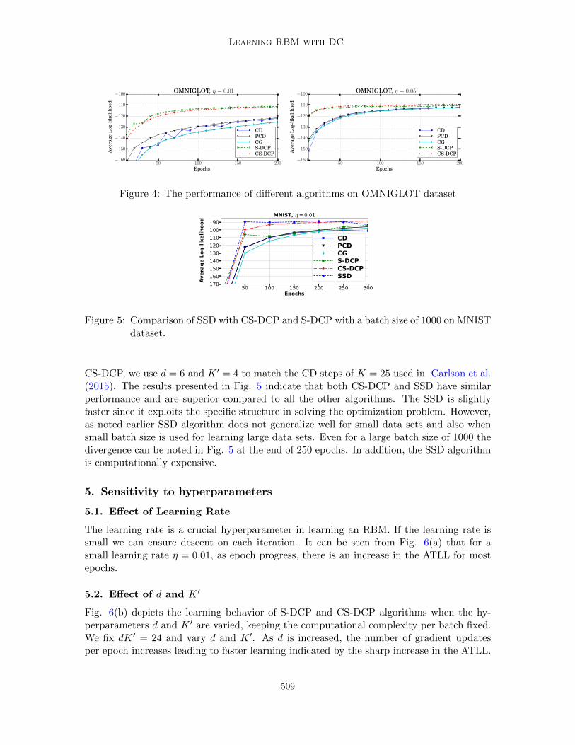
Fig. 3 and Fig. 4 show the results obtained using the MNIST and OMNIGLOT data setsrespectively. For the MNIST dataset, we observe that CS-DCP converges faster when asmall learning rate is used. However, all the algorithms achieve almost the same ATLL atthe end of 200 epochs. For the OMNIGLOT dataset, we see that both S-DCP and CS-DCPalgorithms are superior to all the other algorithms both in terms of speed and the achievedATLL.

The experimental results obtained on these two data sets indicate that both S-DCPand CS-DCP perform well even when the dimension of the model is large. Their speed oflearning is also superior to that of other standard algorithms. For example, when η = 0.01the CS-DCP algorithm achieves 90% of the maximum ATLL approximately 100 epochsbefore the CG algorithm does as indicated by the vertical lines in Fig. 3.

As mentioned earlier, we use batch size 1000 to compare the S-DCP and CS-DCP withthe SSD algorithm. We use exactly the same settings as used in Carlson et al. (2015) andreport the performance on the statistically binarized MNIST dataset. For the S-DCP and

508

Learning RBM with DC

50 100 150 200Epochs

−160

−150

−140

−130

−120

−110

−100

Ave

rage

Log

-lik

elih

ood

OMNIGLOT, η = 0.01

CDPCDCGS-DCPCS-DCP

50 100 150 200Epochs

−160

−150

−140

−130

−120

−110

−100

Ave

rage

Log

-lik

elih

ood

OMNIGLOT, η = 0.05

CDPCDCGS-DCPCS-DCP

Figure 4: The performance of different algorithms on OMNIGLOT dataset

50 100 150 200 250 300Epochs

−170−160−150−140−130−120−110−100−90

Ave

rage

Log

-like

lihoo

d

MNIST, η=0.01

CDPCDCGS-DCPCS-DCPSSD

Figure 5: Comparison of SSD with CS-DCP and S-DCP with a batch size of 1000 on MNISTdataset.

CS-DCP, we use d = 6 and K ′ = 4 to match the CD steps of K = 25 used in Carlson et al.(2015). The results presented in Fig. 5 indicate that both CS-DCP and SSD have similarperformance and are superior compared to all the other algorithms. The SSD is slightlyfaster since it exploits the specific structure in solving the optimization problem. However,as noted earlier SSD algorithm does not generalize well for small data sets and also whensmall batch size is used for learning large data sets. Even for a large batch size of 1000 thedivergence can be noted in Fig. 5 at the end of 250 epochs. In addition, the SSD algorithmis computationally expensive.

5. Sensitivity to hyperparameters

5.1. Effect of Learning Rate

The learning rate is a crucial hyperparameter in learning an RBM. If the learning rate issmall we can ensure descent on each iteration. It can be seen from Fig. 6(a) that for asmall learning rate η = 0.01, as epoch progress, there is an increase in the ATLL for mostepochs.

5.2. Effect of d and K ′

Fig. 6(b) depicts the learning behavior of S-DCP and CS-DCP algorithms when the hy-perparameters d and K ′ are varied, keeping the computational complexity per batch fixed.We fix dK ′ = 24 and vary d and K ′. As d is increased, the number of gradient updatesper epoch increases leading to faster learning indicated by the sharp increase in the ATLL.

509

Upadhya Sastry

(a)50 100 150 200

Epochs

−115

−110

−105

−100

−95

−90

−85

Ave

rage

Log

-lik

elih

ood

MNIST, batch size = 200

S-DCP- η = 0.01CS-DCP-η = 0.01S-DCP- η = 0.03CS-DCP-η = 0.03S-DCP- η = 0.05CS-DCP-η = 0.05

(b)50 100 150 200

Epochs

−115

−110

−105

−100

−95

−90

−85

Ave

rage

Log

-lik

elih

ood

MNIST, batch size = 200, η = 0.01

S-DCP- d = 8,K ′ = 3CS-DCP-d = 8,K ′ = 3S-DCP- d = 6,K ′ = 4CS-DCP-d = 6,K ′ = 4S-DCP- d = 4,K ′ = 6CS-DCP-d = 4,K ′ = 6S-DCP- d = 3,K ′ = 8CS-DCP-d = 3,K ′ = 8

Figure 6: Comparison of S-DCP and CS-DCP algorithms with different (a) learning ratesand (b) values of d and K ′ keeping dK ′ = 24.

However, irrespective of the values d and K ′ both the algorithms converge eventually to thesame ATLL. We find a similar trend in the performance across other data sets as well.

In a way, the above behavior is one of the major advantages of the proposed algorithm.For example, if a longer Gibbs chain is required to obtain a good representative samplesfrom a model, it is better to choose a smaller d and a larger K ′. In such scenarios, theS-DCP and CS-DCP algorithms provide a better control on the dynamics of learning.

5.3. Effect of Batch Size

A small batch size is suggested in Hinton (2010) for better learning with a simple SGDapproach. However, in Carlson et al. (2015), advantages of using a large batch size ofthe order of 2m (twice the number of hidden units) with a well designed optimization, isdemonstrated. If we fix the batch size, then the learning rate can be fixed through cross-validation. However, to analyse the effect of batch size on S-DCP and CS-DCP learning,we fix the learning rate, η = 0.01, and then vary the batch size. As shown in Fig. 7(a), theS-DCP eventually reaches almost the same ATLL, after 200 epochs of training, irrespectiveof the batch size considered. Therefore, the proposed S-DCP algorithm is found to be lesssensitive to batch size. We observed a similar behavior with the Omniglot dataset.

5.4. Sensitivity to Initialization

We initialize the weights with samples drawn from a Gaussian distribution having meanzero and standard deviation, σ. We consider a total of four cases: σ = 0.01 and σ = 0.001and the biases of the visible units are initialized to zero or to the inverse sigmoid of thetraining sample mean (termed as base rate initialization). It is noted in Hinton (2010) thatinitializing the visible biases to the sample mean improves the learning behavior. The biasesof the hidden units are set to zero in all the experiments.

The results shown in Fig. 7(b) indicate that both S-DCP and CS-DCP algorithms areless sensitive to the initial values of weights and biases. We observed similar behavior withthe other datasets.

510

Learning RBM with DC

Table 1: Legend Notation for Fig. 7(b).Init 1 Init 2 Init 3 Init 4

σ 0.001 0.01 0.001 0.01b 0 0 base rate base rate

(a)50 100 150 200

Epochs

−115

−110

−105

−100

−95

−90

−85

Ave

rage

Log

-lik

elih

ood

MNIST, η = 0.01

S-DCP- NB = 100CS-DCP-NB = 100S-DCP- NB = 200CS-DCP-NB = 200S-DCP- NB = 600CS-DCP-NB = 600

(b)20 40 60 80 100 120 140

Epochs

−110

−105

−100

−95

−90

Ave

rage

Log

-lik

elih

ood

MNIST, η = 0.01

S-DCP:Init 1S-DCP:Init 2S-DCP:Init 3S-DCP:Init 4CS-DCP:Init 1CS-DCP:Init 2CS-DCP:Init 3CS-DCP:Init 4

Figure 7: MNIST dataset: Learning with different (a) batch sizes (b) Initialization

6. Conclusions and Future Work

A major issue in learning an RBM is that the log-likelihood gradient is to be obtained withMCMC sampling and hence is noisy. There are several optimization techniques proposedto obtain fast and stable learning in spite of this noisy gradient. In this paper, we proposeda new algorithm, S-DCP, that is computationally simple but achieves higher efficiency oflearning compared to CD and its variants, the current popular method for learning RBMs.

We exploited the fact that the RBM log-likelihood function is a difference of convexfunctions and adopted the standard DC programming approach for maximizing the log-likelihood. We used SGD for solving the convex optimization problem, approximately, ineach step of the DC programming. The resulting algorithm is very similar to CD and hasthe same computational complexity. As a matter of fact, CD can be obtained as a specialcase of our proposed S-DCP approach. Through extensive empirical studies, we illustratedthe advantages of S-DCP over CD. We also presented a centered gradient version CS-DCP.We showed that S-DCP/CS-DCP is very resilient to the choice of hyperparameters throughsimulation results. The main attraction of S-DCP/CS-DCP, in our opinion, is its simplicitycompared to other sophisticated optimization techniques that are proposed in literature forthis problem.

The fact that the log-likelihood function of RBM is a difference of convex functions,opens up new areas to explore, further. For example, the inner loop of S-DCP solves aconvex optimization problem using SGD. A proper choice of an adaptable step size couldmake it more efficient and robust. Also, there exist many other efficient techniques forsolving such convex optimization problems. Investigating the suitability of such algorithmsfor the case where we have access only to noisy gradient values (obtained through MCMCsamples) is also an interesting problem for future work.

Acknowledgments

We thank the NVIDIA Corporation for the donation of the Titan X Pascal GPU used forthis research.

511

Upadhya Sastry

References

Shun-ichi Amari, Koji Kurata, and Hiroshi Nagaoka. Information geometry of Boltzmannmachines. IEEE Transactions on neural networks, 3(2):260–271, 1992.

Le Thi Hoai An and Pham Dinh Tao. The DC (difference of convex functions) programmingand DCA revisited with DC models of real world nonconvex optimization problems.Annals of Operations Research, 133(1):23–46, 2005. ISSN 1572-9338. .

Sebastien Bubeck. Convex optimization: Algorithms and complexity. Found. Trends Mach.Learn., 8(3-4):231–357, November 2015. ISSN 1935-8237. .

David Carlson, Volkan Cevher, and Lawrence Carin. Stochastic spectral descent for re-stricted Boltzmann machines. In Proceedings of the Eighteenth International Conferenceon Artificial Intelligence and Statistics, pages 111–119, 2015.

Guillaume Desjardins, Aaron Courville, and Yoshua Bengio. Adaptive parallel temperingfor stochastic maximum likelihood learning of RBMs. arXiv preprint arXiv:1012.3476,2010.

Guillaume Desjardins, Razvan Pascanu, Aaron C. Courville, and Yoshua Bengio. Metric-free natural gradient for joint-training of Boltzmann machines. CoRR, abs/1301.3545,2013.

Asja Fischer and Christian Igel. Empirical analysis of the divergence of Gibbs sam-pling based learning algorithms for restricted Boltzmann machines. In Artificial NeuralNetworks–ICANN 2010, pages 208–217. Springer, 2010.

Asja Fischer and Christian Igel. An introduction to restricted Boltzmann machines. InProgress in Pattern Recognition, Image Analysis, Computer Vision, and Applications,pages 14–36. Springer, 2012.

Yoav Freund and David Haussler. Unsupervised learning of distributions of binary vectorsusing two layer networks. Computer Research Laboratory [University of California, SantaCruz], 1994.

Geoffrey Hinton. A practical guide to training restricted Boltzmann machines. Momentum,9(1):926, 2010.

Geoffrey E Hinton. Training products of experts by minimizing contrastive divergence.Neural computation, 14(8):1771–1800, 2002.

Geoffrey E. Hinton, Simon Osindero, and Yee Whye Teh. A fast learning algorithm for deepbelief nets. Neural Computation, 18:1527–1554, 2006.

Brenden M. Lake, Ruslan Salakhutdinov, and Joshua B. Tenenbaum. Human-level conceptlearning through probabilistic program induction. Science, 350(6266):1332–1338, 2015.ISSN 0036-8075. .

512

Learning RBM with DC

Yann LeCun, Leon Bottou, Genevieve B. Orr, and Klaus-Robert Muller. Effiicient backprop.In Neural Networks: Tricks of the Trade, This Book is an Outgrowth of a 1996 NIPSWorkshop, pages 9–50, London, UK, UK, 1998. Springer-Verlag. ISBN 3-540-65311-2.

Xuesi Ma and Xiaojie Wang. Average contrastive divergence for training restricted Boltz-mann machines. Entropy, 18(1):35, 2016.

David JC MacKay. Information theory, inference, and learning algorithms, volume 7. Cam-bridge university press Cambridge, 2003.

James Martens. Deep learning via hessian-free optimization. In ICML, 2010.

Jan Melchior, Asja Fischer, and Laurenz Wiskott. How to center deep Boltzmann machines.Journal of Machine Learning Research, 17(99):1–61, 2016.

Gregoire Montavon and Klaus-Robert Muller. Deep Boltzmann Machines and the CenteringTrick, pages 621–637. Springer Berlin Heidelberg, Berlin, Heidelberg, 2012. ISBN 978-3-642-35289-8. .

Radford M Neal. Annealed importance sampling. Statistics and Computing, 11(2):125–139,2001.

Christian Igel Oswin Krause, Asja Fischer. Population-contrastive-divergence: Does con-sistency help with RBM training? CoRR, abs/1510.01624, 2015.

Ruslan Salakhutdinov and Geoffrey E Hinton. Deep Boltzmann machines. In AISTATS,volume 1, page 3, 2009.

Ruslan Salakhutdinov and Iain Murray. On the quantitative analysis of deep belief networks.In Proceedings of the 25th international conference on Machine learning, pages 872–879.ACM, 2008.

Paul Smolensky. Information processing in dynamical systems: Foundations of harmonytheory. 1986.

Tijmen Tieleman. Training restricted Boltzmann machines using approximations to the like-lihood gradient. In Proceedings of the 25th international conference on Machine learning,pages 1064–1071. ACM, 2008.

Tijmen Tieleman and Geoffrey Hinton. Using fast weights to improve persistent contrastivedivergence. In Proceedings of the 26th Annual International Conference on MachineLearning, pages 1033–1040. ACM, 2009.

Pierre van de Laar and Bert Kappen. Boltzmann machines and the em algorithm. 1994.

Alan L Yuille, Anand Rangarajan, and AL Yuille. The concave-convex procedure (CCCP).Advances in neural information processing systems, 2:1033–1040, 2002.

513