learning probabilistic finite state automata for opponent ... · master in artificial intelligence...

Master in Artificial Intelligence (UPC-URV-UB)

Master of Science Thesis

Learning Probabilistic Finite State Automata

For Opponent Modelling

Toni Cebrián Chuliá

Advisor/s: René Alquézar and Alberto Sanfeliu

January 17th

, 2011

A Sandra

Contents

1 Introduction 5

1.1 Motivation . . . . . . . . . . . . . . . . . . . . . . . . . . . . . . 5

1.2 Problem definition and goals . . . . . . . . . . . . . . . . . . . . 6

1.3 Thesis overview . . . . . . . . . . . . . . . . . . . . . . . . . . . 7

2 Problem Description 9

2.1 The Game Environment . . . . . . . . . . . . . . . . . . . . . . 9

2.2 Interacting agents . . . . . . . . . . . . . . . . . . . . . . . . . . 10

2.3 Repeated games . . . . . . . . . . . . . . . . . . . . . . . . . . . 11

2.3.1 Games. Normal Form . . . . . . . . . . . . . . . . . . . . 11

2.4 Opponent Modelling . . . . . . . . . . . . . . . . . . . . . . . . 13

2.4.1 Learning a model . . . . . . . . . . . . . . . . . . . . . . 13

2.4.2 Model assumption . . . . . . . . . . . . . . . . . . . . . 14

2.5 Learning the opponent’s transducer . . . . . . . . . . . . . . . . 14

2.5.1 ALERGIA . . . . . . . . . . . . . . . . . . . . . . . . . . 15

2.5.2 MDI . . . . . . . . . . . . . . . . . . . . . . . . . . . . . 15

2.5.3 GIATI algorithm . . . . . . . . . . . . . . . . . . . . . . 15

2.6 Defeating the opponent . . . . . . . . . . . . . . . . . . . . . . . 16

2.6.1 Utility functions . . . . . . . . . . . . . . . . . . . . . . . 16

2.7 Example . . . . . . . . . . . . . . . . . . . . . . . . . . . . . . . 17

3 Learning Probabilistic Finite State Automata 21

3.1 Introduction . . . . . . . . . . . . . . . . . . . . . . . . . . . . . 21

3.2 Symbols, Languages and Grammars . . . . . . . . . . . . . . . . 21

3.3 Finite State Automaton . . . . . . . . . . . . . . . . . . . . . . 22

3.3.1 Quotient Automaton . . . . . . . . . . . . . . . . . . . . 22

3.3.2 Probabilistic Automata . . . . . . . . . . . . . . . . . . . 22

3.4 Algorithms . . . . . . . . . . . . . . . . . . . . . . . . . . . . . . 23

3.4.1 Identifying regular languages . . . . . . . . . . . . . . . . 23

3.4.2 RPNI . . . . . . . . . . . . . . . . . . . . . . . . . . . . 25

3.4.3 ALERGIA . . . . . . . . . . . . . . . . . . . . . . . . . . 27

3.4.4 MDI . . . . . . . . . . . . . . . . . . . . . . . . . . . . . 28

3

4 CONTENTS

4 Opponent Modelling 31

4.1 Defeating an Opponent . . . . . . . . . . . . . . . . . . . . . . . 314.2 The GIATI algorithm . . . . . . . . . . . . . . . . . . . . . . . . 31

4.2.1 Some terminology . . . . . . . . . . . . . . . . . . . . . . 314.2.2 Inferring Finite-State Transducers . . . . . . . . . . . . . 344.2.3 Applying GIATI in the repeated games scenario . . . . . 35

4.3 Markov Decision Processes . . . . . . . . . . . . . . . . . . . . . 354.3.1 Links between Probabilistic Mealy Machines and MDP . 374.3.2 Infinite horizon models . . . . . . . . . . . . . . . . . . . 384.3.3 Finding optimal policies . . . . . . . . . . . . . . . . . . 39

4.4 Summary . . . . . . . . . . . . . . . . . . . . . . . . . . . . . . 40

5 Experiments 43

5.1 The experiments . . . . . . . . . . . . . . . . . . . . . . . . . . 435.2 Prisoner’s Dilemma . . . . . . . . . . . . . . . . . . . . . . . . . 43

5.2.1 Round length . . . . . . . . . . . . . . . . . . . . . . . . 445.2.2 Match length . . . . . . . . . . . . . . . . . . . . . . . . 465.2.3 Alpha . . . . . . . . . . . . . . . . . . . . . . . . . . . . 46

5.3 RoShamBo . . . . . . . . . . . . . . . . . . . . . . . . . . . . . 485.3.1 The experiment . . . . . . . . . . . . . . . . . . . . . . . 48

6 Conclusions 53

6.1 Future work . . . . . . . . . . . . . . . . . . . . . . . . . . . . . 54

A JSON format for a game 57

B Automata for the RoShamBo experiments 59

Chapter 1

Introduction

1.1 Motivation

Artificial Intelligence (AI) is the branch of the Computer Science field thattries to imbue intelligent behaviour in software systems. In the early years ofthe field, those systems were limited to big computing units where researchersbuilt expert systems that exhibited some kind of intelligence. But with theadvent of different kinds of networks, which the more prominent of those isthe Internet, the field became interested in Distributed Artificial Intelligence(DAI) as the normal move.

The field thus moved from monolithic software architectures for its AI sys-tems to architectures where several pieces of software were trying to solve aproblem or had interests on their own. Those pieces of software were calledAgents and the architectures that allowed the interoperation of multiple agentswere called Multi-Agent Systems (MAS). The agents act as a metaphor thattries to describe those software systems that are embodied in a given environ-ment and that behave or react intelligently to events in the environment.

The AI mainstream was initially interested in systems that could be taughtto behave depending on the inputs perceived. However this rapidly showedineffective because the human or the expert acted as the knowledge bottleneckfor distilling useful and efficient rules. This was in best cases, in worst casesthe task of enumerating the rules was difficult or plainly not affordable. Thissparked the interest of another subfield, Machine Learning and its counter partin a MAS, Distributed Machine Learning. If you can not code all the scenariocombinations, code within the agent the rules that allows it to learn from theenvironment and the actions performed.

With this framework in mind, applications are endless. Agents can be usedto trade bonds or other financial derivatives without human intervention, orthey can be embedded in a robotics hardware and learn unseen map config-uration in distant locations like distant planets. Agents are not restricted tointeractions with humans or the environment, they can also interact with otheragents themselves. For instance, agents can negotiate the quality of service of

5

6 CHAPTER 1. INTRODUCTION

a channel before establishing a communication or they can share informationabout the environment in a cooperative setting like robot soccer players.

But there are some shortcomings that emerge in a MAS architecture. Theone related to this thesis is that partitioning the task at hand into agentsusually entails that agents have less memory or computing power. It is noteconomically feasible to replicate the big computing unit on each separateagent in our system. Thus we can say that we should think about our agents ascomputationally bounded , that is, they have a limited amount of computingpower to learn from the environment. This has serious implications on thealgorithms that are commonly used for learning in these settings.

The classical approach for learning in MAS system is to use some variationof a Reinforcement Learning (RL) algorithm [BT96, SB98]. The main ideaaround those algorithms is that the agent has to maintain a table with the per-ceived value of each action/state pair and through multiple iterations obtain aset of decision rules that allows to take the best action for a given environment.This approach has several flaws when the current action depends on a singleobservation seen in the past (for instance, a warning sign that a robot per-ceives). Several techniques has been proposed to alleviate those shortcomings.For instance to avoid the combinatorial explosion of states and actions, insteadof storing a table with the value of the pairs an approximating function like aneural network can be used instead. And for events in the past, we can extendthe state definition of the environment creating dummy states that correspondto the N-tuple (stateN , stateN−1, . . . , stateN−t)

1.2 Problem definition and goals

Given the problems before mentioned this thesis studies the effect of using amodel based approach to learn in a competitive agent environment. In orderto model the environment, in this case, an opposing agent, probabilistic finitestate automata will be employed. This will limit the range of possible hypoth-esis when searching the state space. For illustrative purpose, the environmentwhere our agents will live is an abstraction of a competitive setting modelledas a game theoretic model.

In this thesis we are going to explore the following related issues:

1. Some state-of-the-art algorithms for learning probabilistic automata willbe presented and discussed. Comparison of the learning abilities of eachalgorithm will be under study

2. Agents can be seen as highly complicated transducers. That is, they aresoftware artifacts that after receiving some sensory inputs react to theenvironment performing some actions. How can the implicit transducerthat an agent hides within its machinery be inferred, will be researched.

1.3. THESIS OVERVIEW 7

3. Finally, when a working hypothesis is obtained, this model must be ex-ploited in order to take an advantage in this setup. But our agent hasto keep in mind that this hypothesis might not be the underlying trans-ducer and that some inexactitudes may happen, both in the structure ofthe model or in the current state. How different models of complexitydegrade over time will be studied because we are mainly interested onwinning the agent competition

This Master’s Thesis tries to explore beyond the point where the thesisof David Carmel ended. In his thesis he tries to infer deterministic automatarestricted to an alphabet with only 2 symbols. In this work, the general frame-work is extended by allowing arbitrary alphabet length and by trying to inferstochastic deterministic transducers. We have not been able to find onlinethe before mentioned thesis but the main lines of research can be learned byreading the references [CM96b, CM96a, CM98, CM99].

1.3 Thesis overview

This thesis is organized as follows:

• Chapter 2 outlines the different areas this thesis relies on. A very simpleexample of the steps and computations is used for illustrative purposes.

• Chapter 3 introduces the necessary automata concepts to understandthe building blocks of the methodology and exposes the algorithms usedto learn the PDFA.

• Chapter 4 presents the algorithmic theory that allows to infer trans-ducers using automata. Once we have our working hypothesis of themodel our opponent is using for choosing movements, we should exploitthis knowledge. To that end we show how can transducers be translatedinto and Markov Decision Processes.

• InChapter 5 we study how our setup is able to infer opponent strategiesand the rate and effectiveness of the learning process.

• Chapter 6 presents the conclusions derived from this study

8 CHAPTER 1. INTRODUCTION

Chapter 2

Problem Description

2.1 The Game Environment

In order to test our ideas we need an environment where two competing agentsinteract with each other. Figure 2.1 illustrate all the elements that are involvedin the experimental setup.

Figure 2.1: Two opposing agents, one that learns and the other that has afixed strategy are competing playing the RoShamBo game

Let’s review the main components:

• Agents are playing a repeated game in the sense that is defined by theGame Theory field. Players play simultaneous games emitting symbols,and after seeing the pair of symbols, an external referee assigns payoffs toeach player. In the figure, agents are playing RoShamBo and the symbolsthey can emit are either Paper, Rock or Scissors. The current movement

9

10 CHAPTER 2. PROBLEM DESCRIPTION

gives one point to our learning agent and -1 points to our fixed agentbecause in RoShamBo, Paper wins Rock.

• There are two opposing agents. In the figure they are represented bythe letters A and B. The B -agent is the agent we are trying to model.It has a probabilistic Moore Machine as its inner core strategy shown inthe upper right cloud. That strategy is fixed and will not change duringthe game and is governed by the symbols that the A-agent sends.

• The A-agent is our learning agent. After some iterations with the B -agent it creates a model hypothesis depicted in the upper-left cloud. Thisautomaton translates nicely to a transducer which this agent believes isthe strategy of the opposing agent. Once the agent has this hypothesisit devises a counter strategy that is used to play the game until the end

The following sections address each element with more detail.

2.2 Interacting agents

One of the most interesting areas of the Artificial Intelligence field is MultiAgent Systems (MAS). According to [Woo02],

Multiagent systems are systems composed of multiple interactingMAScomputing elements, known as agents.Agents are computer systemswith two important capabilities. First, they are at least to some ex-tent capable of autonomous action of deciding for themselves whatthey need to do in order to satisfy their design objectives. Second,they are capable of interacting with other agents not simply by ex-changing data, but by engaging in analogues of the kind of socialactivity that we all engage in every day of our lives: cooperation,coordination, negotiation, and the like.

Another definition about what an agent is can be found in [RN03]

An agent is anything that can be viewed as perceiving itsenvironment through sensors and acting upon that environmentthrough actuators

A rational agent is an agent that does the right thing according to a perfor-mance measure that evaluates a given sequence of environment states. Notethat the performance measure evaluates environment states, not agent states.We can thus define rationality as dependant on four things:

1. The performance measure that defines the criterion of success

2. The agent’s prior knowledge of the environment

2.3. REPEATED GAMES 11

3. The actions that the agent can perform

4. The agent’s percept sequence to date

This again leads to the definition of a rational agent.

For each possible percept sequence, a rational agent should selectan action that is expected to maximize its performance measure,given the evidence provided by the percept sequence and whateverbuilt-in knowledge the agent has [RN03]

The built-in knowledge is usually called the agent program. This programguides how the agent picks actions based on the environment. Depending onthe procedures used by the agent, agent programs can be classified in fourbasic kinds of agent programs:

1. Simple reactive agents

2. Model-based reactive agents

3. Goal-based agents

4. Utility-based agents

In this thesis we are going to explore Model-based reactive agents. For amore exhaustive explanation of the different kinds of agent programs check[PW04].

When an agent can be ascribed to the model-based reactive paradigm weexpect that the agent should maintain some sort of internal state that dependson the percept history and thereby reflects at least some of the unobservedaspects of the current environment state. In our case, the model of the worldwill be an inferred transducer and the state our agent should maintain is inwhich state our transducer currently is.

2.3 Repeated games

2.3.1 Games. Normal Form

A game [LR57] is a mathematical structure that comprises three elements:

1. A set of rules with the inner working of the game

2. A set of available moves to each player depending on the state of thegame

3. A function with the outcomes depending on the state of the game


A game is usually used to represent a conflict between several contending play-ers. This mathematical formulation allows the researcher to employ mathemat-ics to study the outcome of several policies or strategies. In this thesis, movesfrom each player do not depend on the game state, all movements are avail-able in whichever instant of the game. Moreover, outcomes or payoffs are alsoreadily available when both players perform a move. These constraints allowsus to utilize in this thesis the normal form description of a game. When usingthe normal form, games are described by using a matrix where the columnsshow the available movements for one player and the rows the movements forthe other player. Cell intersections are used to represent the payoffs of eachplayer. When the payoff is different for each player, a tuple is used instead,with the row player payoff as its first element and the column player payoff asits second element.

The competitive interaction between agents can thus be formalized as arepetition of a simple two-player game, where on each movement agents in-teract with each other by simultaneously performing an action. The completeset of pairs of actions can be aggregated to denote the history game. Let’s seesome examples of games.

Prisoner’s dilemma

Prisoner’s dilemma is a two-player game, where each player has two possibleactions A = {c, d} and the payoff for each player, p1, p2 is described in thepayoff matrix 2.1. For the Pirsoner’s Dilemma the game theoretical strategy

c dc (3,3) (0,5)d (5,0) (1,1)

Table 2.1: The payoff matrix for the Prisoner’s dilemma game

is to defect always. This is the optimal strategy for games that only involveone interaction, but for repeated games, it is of the interest of the agents tocooperate in the long run because this strategy rewards the agents the most.

RoShamBo

RoShamBo is a popular game that is seemingly used across cultures to diluci-date minor conflicts or choices. Each player can perform one of three actionsA = {paper, stone, scissors} where each action beats or is beaten by the othertwo actions. This can be explicitly shown in the payoff matrix 2.2.

RoShamBo has no stable strategy neither for the single interaction nor forthe repeated game interactions. It is also a zero sum game where what oneplayer wins, the other player loses.

2.4. OPPONENT MODELLING 13

paper stone scissorpaper (0,0) (1,-1) (-1,1)stone (-1,1) (0,0) (1,-1)

scissor (1,-1) (-1,1) (0,0)

Table 2.2: The payoff matrix for the RoShamBo game

2.4 Opponent Modelling

This thesis is mainly about learning the underlying strategy of an opposingopponent. In game theoretic terms it is called opponent modelling. We wantto infer the most accurate model possible of our opponent because once wehave that picture we can create explicit strategies specially tailored to counteract this opponent’s strategies.

2.4.1 Learning a model

Learning a model of an opponent is a kind of unsupervised learning environ-ment. We do not have a set of labeled pairs of sensory input and opponentstate. Instead what we have is the sensory input, that is the set of actionsexchanged, and the game outcomes that are somehow related to the agent’sstate.

In opponent modelling we are trying to infer an abstracted description ofthe player or the player’s behaviour during the game. Opponent modellingis widely used in domains where the competitive nature of the agents arecentral like in Poker. Opponent modelling techniques are employed there toclassify an opponent in an abstract sense as aggressive, rock or calling station1. Alternatively, opponent modelling can go a step further in granularity andtry to predict whether a given player will call, check or raise in a Poker round.

For learning the opponent’s model, you usually have to employ some kind ofReinforcement Learning algorithm (RL)[SB98]. RL algorithms are algorithmsthat learn which actions our agent has to perform in a given environment toaccomplish a given goal usually modelled as a numerical reward. This fam-ily of algorithms, amongst we can find TD-learning, Q-learning and SARSA[BT96], try to infer a function that goes from the state of environment tothe actions that should be performed. This function can be as simple as atable with pairs state/action or in cases where the combinatorial explosion ofstates and actions make infeasible to store such tables, this function can beapproximated by an auxiliary function flexible enough to model those sub-tleties. Those approximating functions are usually created by training neuralnetworks [Hay08].

1For a more comprehensive poker player descriptions check [Skl99]


2.4.2 Model assumption

In this thesis, our main assumption is that our opposing agent has an algo-rithmically encoded strategy to play the game. This algorithm belongs tothe family of functions that can be described as Stochastic Finite State Trans-ducer (SFST). Basically the model we are assuming is that our opponent reactsto our actions deterministically changing to another state in its automaton.In order for the agent to generate its next action, each state has a discreteprobabilistic distribution where symbols will be generated according to thatdistribution. It is also known as a Stochastic Moore Machine.

Moore machines can be directly translated into Mealy machines and theother way around. For our learning purposes it is more convenient that thisStochastic Moore Machine be described as a Stochastic Mealy Machine sincethis translation allows us to use all the already known machinery to deal withMarkov Decision Processes. Transforming a Moore machine into its Mealycounterpart can be easily accomplished by means of appending the symbolemitted in the state to each of the incoming transitions. Since the Mooremachine is Stochastic, this propagation carries the probability associated andgenerates in turn a Stochastic Mealy Machine.

Let’s see a concrete example. In Figure 2.2 we can see an example of suchMoore machines representing an agent that “almost” always emits the samesymbol that triggered the transition. After performing the output symbol

c = 0 . 9d = 0 . 1

c

c = 0 . 1d = 0 . 9

d

c

d

Figure 2.2: Stochastic Moore Machine

propagation on each step, we obtain the Stochastic Mealy machine that canbe seen in Figure 2.3.

Learning this kind of transducers that represent the computational strategyof the opposing agent will be the objective of the learning agent.

2.5 Learning the opponent’s transducer

In order to learn the opponent transducer, rounds of the game will be playedand the results of each round will conform the training data for our PDFAlearning algorithms. After a PDFA has been obtained and using the GIATI

2.5. LEARNING THE OPPONENT’S TRANSDUCER 15

q0 q1d/d (0.45)

d/c (0.05)

d/c (0.05)

d/d (0.45)

c/c (0.45)

c/d (0.05)c/d (0.05)

c/c (0.45)

Figure 2.3: Transformed Mealy machine from the original Moore machine

algorithm a transducer is also obtained. This transducer is similar to a MarkovDecision Process for which known algorithms for proper control exist.

This thesis is concerned with the comparison of different PDFA learningalgorithms and their effect on the competitive environment of the proposedgames. Two main algorithms are going to be studied, ALERGIA and MDI.

2.5.1 ALERGIA

The ALERGIA algorithm by Carrasco and Oncina [CO94] is an extension ofthe non-stochastic algorithm RPNI presented in [Onc92].

2.5.2 MDI

The MDI algorithm ([Tho00]) is conceptually similar to the ALERGIA al-gorithm but improves results by taking into account global features whereasALERGIA is concerned in local ones.

2.5.3 GIATI algorithm

After obtaining an automaton, we use the GIATI algorithm for obtaining thetransducer. In order to learn the Stochastic Finite State Transducer

SFST we employ the GIATI algorithm described in [CVP05]. Given an inputalphabet Σ and an output alphabet ∆ our training corpus consist of wordsformed by (s,t) ∈ Σ+ ×∆+

1. Each training pair (s,t) is transformed into a string z from an extendedalphabet Γ (strings of Γ-symbols) yielding a sample S of strings Z ∈ Γ∗

2. A stochastic regular grammar G is inferred from S

3. The Γ-symbols of the grammar rules are transformed back into pairs ofsource/target symbols/strings (from Σ∗ ×∆∗).

The main problem using the GIATI algorithm is that the mapping fromthe training pairs to the new alphabet, the labeling function L : Σ∗×∆∗ → Γ∗


and the inverse function are not specified and they must make sense in theproblem at hand. In our problem, we don’t have such nuances since, in thegames we are studying, both agents perform only one action on each turn andthus, no problem of alignment between strings has to be inferred.

In Figure 2.4 we can see the machine presented in Section 2.4.2 transformedinto its equivalent Probabilistic Deterministic Finite State Machine over thenew vocabulary Γ : {cc, cd, dc, dd} ≡ {x, y, w, z}.

q0 q1z (0.45)

w (0.05)

w (0.05)

z (0.45)

x (0.45)

y (0.05)y (0.05)

x (0.45)

Figure 2.4: The Mealy Machine has been transformed into a Probabilistic DFAwith an extended alphabet

2.6 Defeating the opponent

Once we have an opponent’s model hypothesis, our task is to generate thecorresponding actions that helps us to govern the automaton. This is easilyaccomplished given the fact that a Mealy Machine, a transducer, can be easilyconverted to an equivalent Markov Decision Process. So our first step willbe to perform that conversion and after that use one of the algorithms forinferring the best policy for the MDP.

2.6.1 Utility functions

In order to solve the best response problem we have to define the utility functionthat our agent is going to use to evaluate a result. This utility function isrelated to each of the payoffs on each game stage and to the remaining horizonin the whole game.

There are several possible utility functions that drive the search of actionsin the MDP, here are a couple for illustrative purposes.

• The discounted-sum function:

Udsi (s1, s2) = (1− γi)

∞∑

t=0

γtiui(s1(g(s1,s2)(t)), s2(g(s1,s2)(t)))

Where Ui is the utility function for player i when hi is playing accordingto strategy s1 and his opponent is using strategy s2.

2.7. EXAMPLE 17

• The limit-of-the-means functions:

U lmi (s1, s2) = lim

k→∞

inf1

k

k∑

t=0

ui(s1(g(s1,s2)(t)), s2(g(s1,s2)(t)))

Where again, Ui is the utility function for player i when he is playingaccording to strategy s1 and his opponent is using strategy s2.

2.7 Example

To illustrate all the process involved, let’s develop an example. Each step willbe explained in further detail in next sections, this is a high level summary ofthe info that has to come.

Let’s start assuming that our agents are competing in a Prisoner’s Dilemmacompetition. The agent that has the fixed strategy is playing the probabilisticTit-For-Tat strategy. That means that this agent, almost always, repeats yourlast move. This agent has been seen before in Figure 2.2 and we reproduce ithere for easiness in following the explanation (Figure 2.5).

q0 q1d/d (0.45)

d/c (0.05)

d/c (0.05)

d/d (0.45)

c/c (0.45)

c/d (0.05)c/d (0.05)

c/c (0.45)

Figure 2.5: Probabilistic transducer (Tit-for-Tat)

Since this is our first iteration, our learning agent has no information aboutwhat is the structure of its opponent, so the best approach is to generatemovements at random. The initial structure can be seen in Figure 2.6. Keep in

q0

c (0.5)

d (0.5)

Figure 2.6: Random Automata

mind, that our random automaton is only a concise way to represent a uniform


distribution of symbols. For our learning agent the model used to generatemovements can be whatever structure, automata, functions or a translationtable.

Let’s advance some terminology. Our objective, is that our learning agentoutperforms its opponent in a Game. A game is composed of several rounds.Each round has a fixed number of matches with a fixed number of movementsfor each match (Figure 2.7) where each agent picks a symbol, and a reward isgiven as an answer of this action. For our example, the game will consist ontwo rounds with 25 moves each distributed on 5 matches per round.

Figure 2.7: Decomposition of each game in several layers of detail

The history of the first 5 matches happens to be:

(d-d)

(c-d)

(c-c)

(c-c)

(d-d)

---------

(d-d)

(d-d)

(c-d)

(d-c)

(d-d)

---------

(d-d)

(d-d)

(c-d)

(d-d)

(d-d)

2.7. EXAMPLE 19

---------

(d-d)

(d-d)

(c-d)

(c-c)

(d-c)

---------

(c-d)

(c-c)

(d-c)

(d-d)

(d-d)

---------

where each tuple represents a simultaneous move of the agents. At thismoment, the game referee stops the exchange of movements, packs the historyobtained so far and notifies it to the learning Agent. Our learning, agentperforms the language transformation of the implicit transducer and groupsletters into words. The resulting word set is

zxwwz

zzxyz

zzxzz

zzxwy

xwyzz

Note, that the learning stage occurs over the extended alphabet.When running the ALERGIA algorithm with parameter α = 0.7 over this

training set we obtain the PDFA in Figure 2.8

0

x [0.26]z [0 .47]

1w [0 .16]

y [0 .053]

w [0 .091]y [0.18]z [0 .36]

Figure 2.8: PDFA learned after the first 25 interactions

But don’t forget that this automaton is representing the Mealy machinethat can be seen in Figure 2.9

The cautious reader should have noticed that outgoing probability transi-tions in this automaton do not add 1. This is so because algorithms learning


0

c/d [0.26]d/d [0.47]

1c/c [0.16]

d/c [0.053]

c/c [0.091]d/c [0.18]d/d [0.36]

Figure 2.9: Mealy Machine derived from the learned PDFA

State Action

0 c1 d

Table 2.3: Derived actions of each state given the Mealy-Machine of Figure2.10

PDFA take into account a transition probability to hidden sink state used tomark the end of the word. Since in our scenario there is no such concept wordwe must smooth the obtained automata in order to normalize the outgoingprobabilities. The final Mealy machine can be seen in 2.10.

0

c/d [0.28]d/d [0.50]

1c/c [0.17]

d/c [0.05]

c/c [0.14]d/c [0.29]d/d [0.57]

Figure 2.10: Smoothed Mealy Machine derived from the learned PDFA

Later in this thesis 4.3.1 it is shown that this probabilistic Mealy Machinecorresponds with a Markov Decision Process for which algorithms exists thatallows us to govern it optimally. Applying a policy iteration algorithm toinfer our decision rules and using the discounted infinite reward function asthe accumulated reward function, we obtain that for this automaton the rulesgoverning the automaton are the ones in Table 2.3.

Chapter 3

Learning Probabilistic Finite

State Automata

3.1 Introduction

The fundamental mathematical object in this thesis is a Finite State Machine,in its different flavors, deterministic, non-deterministic, probabilistic or anextended version, the transducer. It is thus necessary to explain some relatedconcepts about languages and automata.

3.2 Symbols, Languages and Grammars

The field of Syntactic Pattern Recognition is concerned about finding structurein a stream of discrete symbols. Symbols are the elements of a finite set. Thoseelements are usually represented by letters and the set itself is called alphabetand is usually represented by the symbol Σ.

A word is a finite sequence of symbols in a given alphabet. For conveniencethe empty word is also defined and is usually represented by the greek symbolλ. The set of all the words that can be composed by a given alphabet is calledthe universal language of Σ. This language Σ∗ also includes the empty word.So for example, given the alphabet consisting of a single letter Σ = {a}, theuniversal language that can be constructed is:

Σ∗ = {λ, a, aa, aaa, · · · }

Let’s call language over the alphabet Σ to a subset of the universal languageof Σ.

L ∈ Σ∗

We call probabilistic or stochastic language to the pair of a language and afunction that assigns probabilities to each word of the language

{L, PL(·)}

21

22CHAPTER 3. LEARNING PROBABILISTIC FINITE STATE AUTOMATA

3.3 Finite State Automaton

A finite state automaton (FSA) [HMU01, ASMO97], is defined by a five-tuple(Q,Σ, δ, q0, F ) where:

• Q is a finite set of states

• Σ is an alphabet

• q0 is the initial state

• F ⊆ Q is the set of final states

• δ : Q× Σ→ 2Q is a partial function

We say that q is a successor of p if p ∈ δ(q, a). We call our automatondeterministic if for all q ∈ Q and for all a ∈ Σ, the transition δ(q, a) has atmost one element.

3.3.1 Quotient Automaton

Let A be a FSA and π a partition of Q, we denote by B(q, π) as the only blockthat contains q and we denote the quotient set {B(q, π)|q ∈ Q} as Q/π. Givena FSA A and a partition π over Q we define the quotient automaton A/π as:

A/π = (Q/π,Σ, δ′, B(q0, π), {B ∈ Q/π|B ∩ F 6=})

where δ′ is defined as:

∀B,B′ ∈ Q/π, ∀a ∈ Σ, B′ ∈ δ′(B, a) if ∃q, q′ ∈ Q, q ∈ B, q′ ∈ B′ : q′ ∈ δ(q, a)

Given the automaton A and the partition π over Q, we have that the languagedefined by the quotient automaton satisfies L(A) ⊆ L(A/π).

3.3.2 Probabilistic Automata

All the concepts explained for simple automata can be extended to the prob-abilistic case. A stochastic finite automaton (SFA), A = (Σ, Q, P, q0), consistsof an alphabet Σ, a finite set of nodes Q = {q0, q1, . . . , qn} with q0 the initialnode, and a set P of probability matrices pij(a) giving the probability of atransition from node qi to node qj led by the symbol a in the alphabet. If wecall pif the probability that the string ends at node qi, the following constraintapplies:

pif +∑

qj∈Q

∑

a∈A

pij(a) = 1

3.4. ALGORITHMS 23

The probability p(w) for the string w to be generated by A is defined by:

p(w) =∑

qj∈Q

p0j(w)pjf

pij(w) =∑

qk∈Q

∑

a∈A

pik(wa−1)pkj(a)

and the language generated by the automaton A is defined as:

L = {w ∈ Σ∗ : p(w) 6= 0}

Those languages generated by means of a SFA are called stochastic regularlaguages. In case the SFA contains no useless nodes1, it generates a probabilitydistribution for the strings in Σ∗:

∑

w∈Σ∗

p(w) = 1

The algorithms that we are going to use to infer the probabilistic automata,are restricted to learn probabilistic deterministic finite automata (PDFA). Thismeans that for every node qi ∈ Q and symbol a ∈ A there exists at most onenode such pij 6= 0. In such cases a transition function h = δ(i, a) can bedefined.

3.4 Algorithms

3.4.1 Identifying regular languages

Here we present some concepts that will be useful when developing later theautomata algorithms.

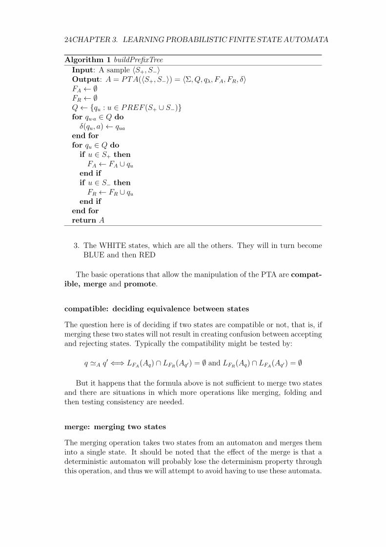
A prefix tree acceptor (PTA) is a tree-like DFA built from the learningsample by taking all the prefixes in the sample as states and constructing thesmallest DFA which is a tree. A formal algorithm buildPrefixTree can be seenin Algorithm 1. Note that we can also build a PTA from a set of positivestrings only. This corresponds to building the PTA(〈S+, ∅〉).

The algorithm we are going to study takes the PTA as a starting point andtries to generalise from it by merging states. In order not to get lost in theprocess it will be interesting to divide the states into three categories:

1. The RED states which correspond to states that have been analysed andwhich will not be revisited; they will be the states of the final automaton

2. The BLUE states which are the candidate states: they have not beenanalysed yet and it should be from this set that a state is drawn in orderto consider merging it with a RED state

1A node qi is useless if there are no strings x, y ∈ Σ∗ such that∑

j p1i(x)pij(y)pjf 6= 0


Algorithm 1 buildPrefixTree

Input: A sample 〈S+, S−〉Output: A = PTA(〈S+, S−〉) = 〈Σ, Q, qλ, FA, FR, δ〉FA ← ∅FR ← ∅Q← {qu : u ∈ PREF (S+ ∪ S−)}for qu·a ∈ Q do

δ(qu, a)← quaend for

for qu ∈ Q do

if u ∈ S+ then

FA ← FA ∪ quend if

if u ∈ S− then

FR ← FR ∪ quend if

end for

return A

3. The WHITE states, which are all the others. They will in turn becomeBLUE and then RED

The basic operations that allow the manipulation of the PTA are compat-

ible, merge and promote.

compatible: deciding equivalence between states

The question here is of deciding if two states are compatible or not, that is, ifmerging these two states will not result in creating confusion between acceptingand rejecting states. Typically the compatibility might be tested by:

q ≃A q′ ⇐⇒ LFA(Aq) ∩ LFR

(Aq′) = ∅ and LFR(Aq) ∩ LFA

(Aq′) = ∅

But it happens that the formula above is not sufficient to merge two statesand there are situations in which more operations like merging, folding andthen testing consistency are needed.

merge: merging two states

The merging operation takes two states from an automaton and merges theminto a single state. It should be noted that the effect of the merge is that adeterministic automaton will probably lose the determinism property throughthis operation, and thus we will attempt to avoid having to use these automata.

3.4. ALGORITHMS 25

promote: promoting a state

Promotion is another deterministic and greedy decision. The idea here is thathaving decided that a state in the PTA that is a candidate for merging withthe final automata state, this state should finally become a final state of theresulting automata and should not be merged.

3.4.2 RPNI

Although not an algorithm to learn Probabilistic DFAs but regular Determin-istic Finite Automata, the algorithm RPNI [Onc92] is the base for the Alergia(3.4.3) and subsequently the MDI algorithm (3.4.4). It is thus interesting tobriefly review how it works.

Although its similarities with its probabilistic derivations, this algorithmneeds both a sample of positive attributes (S+) belonging to the language weare trying to learn and a set of negative examples (S−) that do not belongto the intended language. Obviously, the more examples both positive andnegative, the more is covered the language and thus the easier to learn exactly.

This algorithm starts by building the prefix tree acceptor of the positiveinstances of the training sample (S+) and then proceeds by iteratively choosingpossible merges, checks if a given merge is correct and is made between twocompatible states, makes the merge if admissible and promotes the state if nomerge is possible.

The algorithm has as a starting point the PTA, which is a deterministicfinite automaton. In order to avoid problems with non-determinism, the mergeof two states is immediately followed by a folding operation: the merge inRPNI always occurs between a state already selected as final and a state thatis considered in the iteration.

At the end of the process we expect the obtained automaton to accept thestrings present in the training sample and to reject the negative ones.

Algorithm 2 RPNI-PROMOTE

Input: a DFA A = 〈Σ, Q, qλ, FA, FR, δ〉, sets Red,Blue ⊆ Q, qu ∈ Blue

Output: A, Red, Blue updatedRed← Red ∪ {qu}Blue← Blue ∪ {δ(qu, a), a ∈ Σ}return A, Red,Blue

Example

Here we show how a PTA is built from a set of examples. For this dataset wehave that S+ = {011, 101} and S− = {1, 01}. So the PTA obtained from theset of positive examples can be seen in Figure 3.1.


Algorithm 3 RPNI-COMPATIBLEInput: A, S−

Output: a Boolean, indicating if A is consistent with S−

for w ∈ S− do

if δA(qλ, w) ∩ FA 6= ∅ thenreturn False

end if

end for

return True

Algorithm 4 RPNI-MERGE

Input: a DFA A, states q ∈ Red, q′ ∈ Blue

Output: A updatedLet (qf , a) be such that δA(qf , a) = q′

δA(qf , a)← qreturn RPNI-FOLD(A, q, q′)

Algorithm 5 RPNI-FOLD

Input: a DFA A, states q, q′ ∈ Q q’ being the root of a treeOutput: A updated, where subtree q′ is folded into qif q′ ∈ FA then

FA ← FA ∪ {q}end if

for a ∈ Σ do

if δA(q′, a) is defined then

if δA(q, a) is defined then

A← RPNI-FOLD(A, δA(q, a), δA(q′, a))

else

δA(q, a)← δA(q′, a)

end if

end if

end for

3.4. ALGORITHMS 27

Algorithm 6 RPNI

Input: a sample S = 〈S+, S−〉, functions COMPATIBLE, CHOOSEOutput: a DFA A = 〈Σ, Q, qλ, FA, FR, δ〉A← BUILD-PTA(S+)Red← {qλ}Blue← {qa : a ∈ Σ ∩ Pref(S+)}while Blue 6= ∅ doCHOOSE(qb ∈ Blue)Blue← Blue \ {qb}if ∃qr ∈ Red such that RPNI-COMPATIBLE(RPNI-MERGE(A, qr, qb), S−)then

A← RPNI-MERGE(A, qr, qb)Blue← Blue ∪ {δ(q, a) : q ∈ Red ∧ a ∈ Σ ∧ δ(q, a) /∈ Red}

else

A← RPNI-PROMOTE(qb, A)end if

end while

for qr ∈ Red do

if λ ∈ (L(Aqr)−1S− then

FR ← FR ∪ {qr}end if

end for

λ

0 01 011

1 10 101

01 1

10 1

Figure 3.1: Prefix tree of the positive training sample

3.4.3 ALERGIA

The ALERGIA algorithm [CO94] for learning PDFAs follows the same princi-ples than the RPNI algorithm seen in Section 3.4.2. First begins by buildingthe Prefix Tree Acceptor (PTA) from the training sample and evaluates atevery node the relative probabilities of the transitions coming out from thenode. Next it tries to merge couples of nodes following a well defined order(essentially, that of the levels in the PTA or lexicographical order). Merging isperformed if the resulting automaton is, within statistical uncertainty, equiva-lent to the PTA. The process ends when further merging is not possible. The


algorithm can be seen in Algorithm 9

Algorithm 7 ALERGIA-TEST

Input: an FFA A, f1, n1, f2, n2, α > 0Output: a Boolean indicating if the frecuencies f1

n1and f2

n2are sufficiently

closeγ ← f1

n1− f2

n2

return(

γ <(√

1n1

+√

1n2

)

·√

12ln 2

α

)

The compatibility test makes use of the Hoeffding bounds. The algorithmALERGIA-COMPATIBLE (8) calls the ALERGIA-TEST (7) as many timesas needed, this number being finite due to the fact that the recursive calls visita tree.

The basic function CHOOSE is as follows: take the smallest state in anordering that has been done at the beginning (on the PTA). The test that isused to decide if the states are to be merged or not (function COMPATIBLE)is based on the Hoeffding test made on the relative frequencies of the emptystring and of each prefix.

Algorithm 8 ALERGIA-COMPATIBLEInput: an FFA A, two states qu, qv, α > 0Output: qu and qv compatible?Correct← Trueif ALERGIA-TEST(FP A(qu),FREQA(qu), FP A(qv), α) thenCorrect← False

end if

for a ∈ Σ do

if ALERGIA-TEST(δfr(qu, a),FREQA(qu), δfr(qv, a),FREQA(qv), α)then

Correct← Falseend if

end for

3.4.4 MDI

Algorithm ALERGIA decided upon merging (and thus generalisation) througha local test: substring frequencies are compared and if it is not unreasonableto merge, then merging takes place. A more pragmatic point of view couldbe to merge whenever doing so is going to give us an advantage. The goalis of course to reduce the size of the hypothesis while keeping the predictivequalities of the hypothesis (at least with respect to the learning sample) asgood as possible. For this we can use the likelihood of each string. The goal isto obtain a good balance between the gain in size and the loss in perplexity.

3.4. ALGORITHMS 29

Algorithm 9 ALERGIA

Input: a sample S, α > 0Output: an FFA ACompute t0, threshold on the size of the multiset needed for the test to bestatistically significantA← PTA(S)Red← {qλ}Blue← {qa : a ∈ Σ ∩ Pref(S)}while CHOOSE(qb) from Blue such that FREQ(qb) ≥ t0 do

if ∃qr ∈ Red : ALERGIA-COMPATIBLE(A, qr, qb, α) thenA← STOCHASTIC-MERGE(A, qr, qb)

else

Red← Red ∪ {qb}end if

Blue← {qua : ua ∈ Pref(S) ∧ qu ∈ Red} \Red

end while

return A

Attempting to find a good compromise between these two values is themain idea of algorithm MDI (Minimum Divergence Inference).

Algorithm 10 MDI-COMPATIBLE

Input: an FFA A, two states q and q′, S, α > 0Output: a Boolean indicating if q and q′ are compatibleB ← STOCHASTIC-MERGE(A, q, q′)return (score(S,B) < α)

The key difference is that the recursive merges are made inside AlgorithmMDI-COMPATIBLE (3.4.4) and before the new score is computed instead ofin the main algorithm.

Like in the ALERGIA algorithm, a difficult question to answer is that ofsetting the tuning parameter (α): if set too high, merges will take place early,which will perhaps include a wrong merge, prohibiting later necessary merges,and the result can be bad. On the contrary, a small α will block all merges,including those that should take place, at least until there is little data left.This is the safe option, which leads in most cases to very little generalization.


Algorithm 11 MDI

Input: a sample S, α > 0Output: an FFA ACompute t0, the threshold on the size of the multiset needed for the test tobe statistically significantA← PTA(S)Red← {qλ}Blue← {qa : a ∈ Pref(S)currentscore← score(S, PTA(S))while CHOOSE(qb) from Blue such that FREQ(qb) ≥ t0 do

if ∃qr ∈ Red : MDI-COMPATIBLE(A, qr, qb, S, α) thenA← STOCHASTIC-MERGE(A, qr, qb)

else

Red← Red ∪ {qb}end if

Blue← {qua : ua ∈ Pref(S) ∧ qu ∈ Red} \Red

end while

return A

Chapter 4

Opponent Modelling

4.1 Defeating an Opponent

In Chapter 3 we learned about the algorithms used for inferring the PDFAs.Those algorithms are used in the context of a repeated game setup where ourlearning agent is trying to defeat an opponent. This chapter is about the twomain steps that must be performed to accomplish this goal:

1. Derive a working hypothesis about the internal strategy that our oppo-nent is using. This will be accomplished using the GIATI algorithm.

2. Derive a counter-strategy that could exploit any weaknesses that strategycould have. This will be accomplished translating our working hypothesisinto a Markov Decision Process and deriving the governing rules for it.

4.2 The GIATI algorithm

In the previous chapter we have seen techniques to infer probabilistic automatafrom examples but in this thesis what we are trying to infer is the transducerthat our opponent is using to play the game. So, we should fill the gap betweenhaving algorithms that learn PDFAs and to convert those models into thetarget transducer. This chapter is devoted to the necessary techniques toaccomplish this task.

4.2.1 Some terminology

A finite-state transducer (FST), T , is a tuple 〈Σ,∆, Q, q0, F, δ〉, in which:

1. Σ is a finite set of source symbols

2. ∆ is a finite set of target symbols

3. Q is finite set of states

31

32 CHAPTER 4. OPPONENT MODELLING

4. q0 is the initial state

5. F ⊆ Q is a set of final states

6. δ ⊆ Q× Σ×∆∗ ×Q is a set of transitions.

Note that Σ ∩∆ = ∅. A translation form φ of length I in T is defined as thesequence of transitions:

φ = (qφ0 , sφ1 , t

φ1 , q

φ1 )(q

φ1 , s

φ2 , t

φ2 , q

φ2 ) · · · (q

φI−1, s

φI , t

φI , q

φI )

where (qφi−1, sφi , t

φi , q

φi ) ∈ δ. A pair (s, t) ∈ Σ∗×∆∗ is a translation pair if there

is a translation form φ of length I in T such that I = |s| and t = tφ1 tφ2 · · · t

φI .

A rational translation is the set of all translation pairs of some finite-statetransducer T .

This definition of a finite-state transducer is similar to the definition of aregular or finite-state grammar. The main difference is that in a finite-stategrammar, the set of target symbols ∆ does not exist, and the transitions aredefined on Q × Σ × Q. A translation form is the transducer counterpart of aderivation in a finite-state grammar, and the concept of rational translation isreminiscent of the concept of (regular) language, defined as the set of stringsassociated with the derivations in the grammar G.

A stochastic finite-state transducer , TP is defined as a tuple 〈Σ,∆, Q, q0, p, f〉in which Q, q0,∆,Σ are as in the definition of a finite-state transducer and pand f are two functions:

1. p : Q× Σ×∆∗ ×Q→ [0, 1]

2. f : Q→ [0, 1]

That satisfy ∀q ∈ Q

f(p) +∑

(a,w,q′)∈Σ×∆∗×Q

p(q, a, w, q′) = 1

The probability of a translation pair (s, t) ∈ Σ∗ ×∆∗ according to TP

is the sum of the probabilities of all the translation forms of (s, t) in T :

PTP(s, t) =

∑

φ∈d(s,t)

PTP(φ)

where the probability of a translation form φ is

PTP(φ) =

I∏

i=0

p(qi−1, si, ti, qi) · f(qI)

that is, the product of the probabilities of all the transitions involved in φ.

4.2. THE GIATI ALGORITHM 33

There are two main types of finite state transducers, the Moore machineand the Mealy machine. Since we are interested in its stochastic derivations,we will show the definition of the probabilistic instances. The definition ofthe deterministic entities could be obtained by simply taking into accountdegenerate probabilities where only one transition has the full weight, i.e. thereis a transition that has probability 1.

Moore machine

A Moore machine is a deterministic automaton with the ability to generatesymbols. Like other automata, the Moore machine performs state transitionsdepending on the input symbol consumed. When the automata lands in a newstate, an output symbol is generated according to an internal formula.

Formally a stochastic Moore machine is a tuple 〈Q,Σ,∆, δ, λ, q0〉 where:

• Q is the set of nodes in the automaton

• Σ and ∆ are the input and output alphabets

• δ : Q× Σ→ PQ is the set of probability distributions over Q

• λ : Q → P∆ is the probabilistic output function. The Moore machinegenerates output symbols according to a given probability function P∆


Mealy machine

A Mealy machine is also a deterministic automaton that generates outputsymbols during the state transition. The main difference with the Mooremachine is that you can define different probability functions for the transitionsand for the output symbols while in the Mealy machine the probability functionis a joint function for the transitions and the output symbols.

Mathematically a Mealy machine is a tuple 〈Q,Σ,∆, δ, q0〉 where:

• Q is the set of nodes in the automata

• Σ and ∆ are the input and output alphabets

• δ : Q × Σ → PQ×∆ is the set of probability distributions over the set oftransitions and output symbols Q×∆


The GIATI algorithm relies on the following two theorems. The interestedreader should check [Ber09] for the corresponding proofs.

Theorem 4.1. T ⊆ Σ∗×∆∗ is a rational translation if and only if there existsan alphabet Γ, a regular language L ⊂ Γ∗, and two morphisms hΣ : Γ∗ → Σ∗

and h∆ : Γ∗ → ∆∗ such that T = {(hΣ(w), h∆(w))|w ∈ L}.


and

Theorem 4.2. A distribution PT : Σ∗ × ∆∗ → [0, 1] is a stochastic rationaltranslation if and only if there exist an alphabet Γ, two morphism hΣ : Γ∗ → Σ∗

and h∆ : Γ∗ → ∆∗, and a stochastic regular language PL such that ∀(s, t) ∈Σ∗ ×∆∗,

PT (s, t) =∑

w∈Γ∗:(hΣ(w),h∆(w))=(s,t)

PL(w)

4.2.2 Inferring Finite-State Transducers

The methodology explained in [CV04] is called grammatical inference and

alignment for transducer inference (GIATI). Based on the works of Berstel[Ber09] it is well known that (stochastic) rational translation T can be obtainedas a homomorphic image of certain (stochastic) regular language L over anadequate alphabet Γ.

This suggest the following general technique for learning a stochastic finite-state transducer, given a finite sample I+ of string pairs (s, t) ∈ Σ∗ ×∆∗:

1. Each training pair (s, t) from I+ is transformed into a string z from anextended alphabet Γ (strings of Γ-symbols) yielding a sample S of stringsS ⊂ Γ∗. Lets call this transformation L : Σ∗ ×∆∗ → Γ∗

2. A (stochastic) regular grammar G is inferred from S

3. The Γ-symbols of the grammar rules are transformed back into pairs ofsource/target symbols/strings (from Σ∗ × ∆∗). The “inverse labellingfunction” Λ : Γ∗ → Σ∗ × ∆∗ is one that Λ(L(I+)) = I+. FollowingTheorems 4.2 and 4.1, Λ(·) consists of a couple of morphisms, hΣ, h∆,such that for a string z ∈ Γ∗, Λ(z) = (hΣ(z), h∆(z))

The overall procedure can be seen in the Figure 4.1.

A ⊂ Σ∗ ×∆∗Labeling - L(·)−−−−−−−−→ S ⊂ Γ∗

yGI

y

algorithm

T : A ⊂ T (T)Inverse labeling - Λ(·)←−−−−−−−−−−−− G : S ⊂ L(G)

Figure 4.1: Commutative diagram of the transformations performed using theGIATI algorithm

4.3. MARKOV DECISION PROCESSES 35

4.2.3 Applying GIATI in the repeated games scenario

When applying the GIATI algorithm three placeholders have to be filled inorder to run the algorithm, the labelling function L(·), the inverse labellingfunction Λ(·) and the algorithm used to learn the probabilistic automaton.For our opponent modelling scenario that has been defined in Section 2.3, theGIATI elements are defined as follows:

• Choosing the labelling function L tends to be a difficult decision. In sta-tistical translation, that is one of the domains where FST are of commonuse, a previous study of the statistical correlations between the positionsof the words in the source language and the target language, called sta-tistical alignment, is performed. In our case, since the action and theresponse are always paired, there is no need to perform such statisticalanalysis of the data, each input symbol is paired with only one outputsymbol.

So, the labelling function L will be

L(s, t) = concat(s, t) = st = z z ∈ Γ

where the symbol st ∈ Γ is obtained from the alphabet Γ that receivesits elements from all the permutations of the symbols in Σ and ∆.

• Learning the probabilistic automata will be performed using one of thebefore mentioned algorithms, ALERGIA and MDI

• The inverse labelling function just splits the source symbol from thetarget symbol

Λ(z) = Λ(st) = (s, t) s ∈ Σ, t ∈ ∆

4.3 Markov Decision Processes

A Markov Decision Process (MDP) [Ber95, Put94] consists of five elements:decision epochs, states, actions, transition probabilities, and rewards.

Decision Epochs and Periods

Decisions are made at points of time referred as decision epochs. Let T denotethe set of decision epochs, in a discrete environment T can be finite or infiniteranging in the real positive line. In our discrete environment, at each epochdecisions are made to govern the probabilistic system.


State and Action Sets

At each decision epoch, the system occupies a state. We denote the set ofpossible system states as S. If, at some decision epoch, the decision makerobserves the system in state s ∈ S, he may choose action a from the set ofallowable actions in state s, As. Given this setup let A = ∪s∈SAs. Note thatS and A do not vary with t.

Actions may be chosen either randomly or deterministically. Choosingactions randomly means selecting a probability distribution q(·) ∈ P (As) beingP (As) the collection of probability distributions on subsets of As. When weare dealing with deterministic selection of actions, our model is simply usingdegenerate probability distributions.

Rewards and Transition Probabilities

As a result of choosing action a ∈ As in state s,

1. the decision maker receives a reward, rt(s, a) and

2. the system state at the next decision epoch is determined by the proba-bility distribution p(·|s, a)

From the perspective of the models, it is immaterial how the reward isaccrued during the period. We only require that its value or expected value beknown before choosing an action, and that it not be effected by future actions.The reward might be,

1. a lump sum received prior to the next decision epoch

2. a random quantity that depends on the system state at the subsequentepoch

3. or a combination of the above

When the reward depends on the state of the system at the next decisionepoch, we let r(s, a, j) denote the value at time t of the reward received whenthe sttate of the system at decision epoch t is s, action a ∈ As is selectedand the system occupies state j at decision epoch t+ 1. Its expected value atdecision epoch t may be evaluated by computing

rt(s, a) =∑

j∈S

rt(s, a, j)pt(j|s, a)

We usually assume that∑

j∈S

pt(j|s, a) = 1

We refer to the collection of objects forming a tuple

〈T, S,As, p(·|s, a), r(s, a, j)〉 (4.1)


as a Markov Decision Process. The qualifier “Markov” is used because thetransition probabilities and reward functions depend on the past only throughthe current state of the system and the action selected by the decision makerin that state.

Decision Rules

A decision rule prescribes a procedure for action selection in each state ata specified decision epoch. There is a lot of variety on how decision rulespick their actions but the primary focus in this thesis will be on deterministicMarkovian rules because they are easier to implement and evaluate. Suchdecision rules are functions d : S → As, which specify the action choice whenthe system occupies state s, and thus for each s ∈ S we have d(s) ∈ As. Thisdecision rule is said to beMarkovian (memoryless) because it does not dependson previous system states and actions only thought the current state of thesystem, and deterministic because it chooses an action with certainty.

Policies

A policy specifies the decision rule to be used at all decision epochs. We calla policy stationary if dt = d for all t ∈ T

4.3.1 Links between Probabilistic Mealy Machines and

MDP

The GIATI algorithm provides us with a transducer in the form of a non-deterministic Mealy Machine. There is an almost direct translation betweenthis Mealy machine and an MDP but some considerations should be taken intoaccount. Lets recap the definitions of those mathematical objects, a MealyMachine (Section 4.2.1) is the tuple:

〈Q,Σ,∆, δ, q0〉

and a Markov Decision Process (Equation 4.1) is defined by:

〈T, S,As, p(·|s, a), r(s, a, s′)〉

So the different transformations can be summarized by

• The decision epochs T in a MDP are more general than the step tran-sitions in a transducer since in an MDP, continuous or Borel sets areallowed as epoch. Since we are doing the translation from a Mealy ma-chine to an MDP the translation is direct, the MDP is fixed to discreteand evenly spaced decision epochs and no further adaptations must bedone.


• The set of states Q and S can be used interchangeably between the twomodels. Here we perform a direct translation

• For the transition probabilities in an MDP, p(s′|s, a) some derivationsmust be performed. In a Mealy machine our transition function δ spec-ifies probabilities for the pairs next state plus emitting symbol, Q ×∆,so the basic translation should be

p(s′|s, a) =∑

t∈∆

p(s, a, s′, t)

• The reward function, r(s, a, s′) depends on the game we are playing.When a transition happens in a Mealy machine, both the input symboland the emitted symbol are available. This represents a movement thata referee later will assign a value to each player, so in order to provide anexpected value for a transition, the rewards are weighted by the proba-bilities of a given transition happening when receiving an input symbol

r(s, a, s′) =∑

t∈∆

p(s, a, s′, t) · evalMove(a, t)

Where the function evalMove is game dependent.

With these simple translations, a given Mealy machine obtained by theGIATI algorithm can be translated into a Markov Decision Process, ready forobtaining the governing decision rules.

4.3.2 Infinite horizon models

When a Markov decision process is run indefinitely, each policy induces adiscrete-time reward process. That reward stream has an associated utilityto the agent depending on some functions used to value that stream. Severalfunctions can be used to aggregate that stream into a single value for easinesswhen comparing different streams:

1. The expected total reward policy π, vπ is defined to be

vπ(s) ≡ limN→∞

Eπs

{

N∑

t=1

r(Xt, Yt)

}

= limN→∞

vπN+1(s) (4.2)

Note that the limit in 4.2 may be +∞ or −∞ and consequently thisperformance measure is not always appropriate.

2. The expected discounted reward of policy π is defined to be

vπλ(s) ≡ limN→∞

Eπs

{

N∑

t=1

λt−1r(Xt, Yt)

}

for 0 ≤ λ ≤ 1


3. The average reward or gain of policy π is defined by

gπ(s) ≡ limN→∞

1

NEπ

s

{

N∑

t=1

r(Xt, Yt)

}

The expected total discounted reward criterion

The discounted reward model is the function valuation that will be employedin this thesis. The discounted reward has strong links with the economicbehaviour and decision theoretic literature and our learning agent is dealingwith utility functions to determine which actions to take. Moreover, discountedfunctions present some mathematical niceties that allow easy function usage,we do not need to worry about the convergence of the reward series.

Discounted policy also helps in our game setup since our agent assignsgreater value to rewards closer in time. Although games are not infinite, theagent does not know how long they are going to take and thus a strategy thatassigns uncertainty to distant and future rewards is preferable.

4.3.3 Finding optimal policies

The transitions in a Markov Decision Process are independent of the tran-sition history that took the MDP to a given state and by derivation, it hasno dependency either on the decision that generated the transitions in thefirst place. So the objective is to find a collection of pair state/action, π ={(q0, a0), (q1, a1), · · · , (qS, aS), that defines our policy.

Given a Markov Decision Process we are interested on a policy ππλ

vπ∗

λ = supπ

vπλ(s)

where the expected total discounted reward is defined by

vπλ(s) = Eπs

{

∞∑

t=1

λt−1r(qt, at)

}

Several algorithms exist for finding such policies like value iteration, policyiteration, modified policy iteration and linear programming [Put94, Ber95]. Inthis thesis we will show the two most common procedures value iteration andpolicy iteration.

Value iteration

The main idea behind the value iteration is that the utility of a given state iscomputed iteratively. The procedure guarantees that in the limit, the utilityconverges to its real value. In practice the algorithm does not go to the infinitybut instead stops when the utility does not change above a specified threshold.

In Algorithm 12 the value iteration algorithm can be seen.


Algorithm 12 Value Iteration Algorithm

Input: an MDP M , a threshold εOutput: a function d : states× actionsv0 ← 0, n← 0, S ← states(M)repeat

for all s ∈ S do

vn+1(s) = maxa∈As

{

r(s, a) +∑

j∈S λp(j|s, a)vn(j)

}

end for

until ||vn+1 − vn|| < ε(1− λ)/2λ

return dε(s) ∈ argmaxa∈As

{

r(s, a) +∑

j∈S λp(j|s, a)vn+1(j)

}

Policy iteration

The value iteration algorithm first computes the set of utility functions for eachstate and when those are calculated, it chooses the action that gives best utilityoverall. While value iteration can be regarded as a fixed point algorithm, policyiteration relates directly to the structure of Markov Decision Processes. In thepolicy iteration algorithm, a set of rules is iterated until no change in the rulesprovides better performance. It is known that this procedure provides betterperformance and faster convergence rates.

4.4 Summary

Let’s briefly summarize the steps that our agent takes in order to play thegames.

First it will play a round of games choosing random movements becausethat is the best strategy that can be followed when you have no idea aboutthe opponent’s strategy.

After this first round, all the pairs of movements will be collected. Thosepairs will be transformed to single symbols of an extended alphabet as isexplained in the GIATI algorithm.

With the new set of symbols and the associated words, a PDFA is learned.Once we have this automaton a Mealy Machine is derived using the function torevert symbols from the extended alphabet to pairs of input-output symbols.

The Mealy Machine is then converted to a Markov Decision Process andthe Policy Iteration algorithm is used to derive a set of rules. The rules are adictionary with the action that has to be performed when the Mealy Machineis in a given state.

With the new Mealy Machine and the set of rules the agent plays anotherround of movements.

4.4. SUMMARY 41

Algorithm 13 Policy IterationInput: a MDP MOutput: a policy π with an action for each state in MV (s) ∈ ℜ and π(s) ∈ A(s) randomly chosen for all s ∈ states(M)repeat

// Policy evaluation∆←∞repeat

v ← V (s)

V (s)←∑

s′ Pπ(s)ss′ [R

π(s)ss′ + γV (s′)]

∆← min(∆, |v − V (s)|)until ∆ < ǫ// Policy improvementpolicyStable← truefor all s ∈ S do

b← π(s)

π(s)← argmaxa∑

s′ Pπ(s)ss′ [R

π(s)ss′ + γV (s′)]

if b 6= π(s) thenpolicyStable← false

end if

end for

until policyStable = truereturn π

Chapter 5

Experiments

In the previous chapters, we have delineated the framework that uses PDFAlearning algorithms for controlling an opposing agent in a game setup. Howwell this algorithmic platform works in the task of winning an opponent issomething we will study here.

5.1 The experiments

Here we describe the experimental setup we have used. All the graphs containthe results for each of the algorithms under study (ALERGIA and MDI) plusthe results of using a random player against the opponent. The other measuretaken is how much could we made against the opponent if we knew on each timestep in which state the opponent is and issuing the command most favourableto us.

The software

In order to conduct the experiments that follow we developed a testing frame-work where we could play with different automata and algorithm configuration.The code for the ALERGIA algorithm and the MDI were kindly provided bythe authors [Onc92, Tho00].

5.2 Prisoner’s Dilemma

For the study of the Prisoner’s dilemma game we will use as opponents threedifferent Moore Machine borrowed from the famous tournament held by RobertAxelrod [Axe84]. In the original tournament, fifteen attendees competed inround-robin tournament of the iterated Prisoner Dilemma, where every inter-action was based on 200 repetitions of the PD game. In the study we are goingto use three of the best opponents sent to the tournament. Those opponentscan be seen in Figure 5.1. The automata in the figure must be regarded asMoore Machines. Here we haven’t explicitly stated the emitting symbols and

43

44 CHAPTER 5. EXPERIMENTS

TTT c

c

d

d

c

d

Tf2T c

c

cd

c

d

d

c

d

Nydegger c

c

c

d

d

c

d

d d

c

d

d

d

c

cd

c

d

c

dd

c

c

cd

c

d

d

c

d

c

c

cd

d

c

Figure 5.1: Prisoner’s Dilemma opponents used in the study

probabilities in order to not clutter the diagram. The labels on each state mustbe regarded as the prevailing emitting symbol, that is, a c represents that astate has probabilities Pstate(c) = 0.9 and Pstate(d) = 0.1, and conversely, a d

represents Pstate(c) = 0.1 and Pstate(d) = 0.9. The exact numbers of the proba-bilities were chosen in order to introduce a meaningful probabilistic behaviourin the automata keeping at the same time its original intended purpose dueto its architecture. Here are a brief description of the meaning of each of theautomata:

• Tit-for-Tat (TTT): Cooperates at the first iteration and then follows(most likely) the previous opponent’s action.

• Tit-for-two-Tat: Tf2T Cooperates (most likely) for the two first statesand defects (most likely) after two consecutive defections of its opponent.

• Nydegger Behaves like TTT at the beginning and then behaves accord-ing to the three previous joint actions of both players.

5.2.1 Round length

In this set experiments we want to study the effect of the round length inthe game outcome. On each round a new agent hypothesis is created withthe movements of this round. So the best agent that we could obtain wouldbe the one learnt after the full game happens, but this would leave us withthe random player playing all the movements in the beginning and we areprimarily interested in wining the game. So a balance or trade-off has tobe found for better performance. This section will study how increasing the

5.2. PRISONER’S DILEMMA 45

Figure 5.2: Average payoff against different opponents when we vary the num-ber of rounds in the game


number of rounds for a fixed number of movements affects the quality of thegame results.

Figure 5.2 shows that on average, MDI algorithm performs better thatALERGIA taking into account the average payoff per move. Both algorithmsseems to improve with the number of rounds, till we arrive at 10 rounds pergame, where the improvement stabilizes. One remarkable thing is that whencompeting against the Tf2T opponent, the random player performs better thanwhichever of our algorithms. This is because of the structure of the opponentand the chosen payoffs for the Prisoner’s dilemma game. The opponent reactsto 2 consecutive defections with the defect action, but it returns to the coop-erative setting whenever a cooperation happens. Given the payoffs the mostprofitable strategy could be to alternate defections and cooperations on eachsingle state, but our agent can’t learn this strategy because it can not querywhich moves it issued (that would break our MDP hypothesis also).

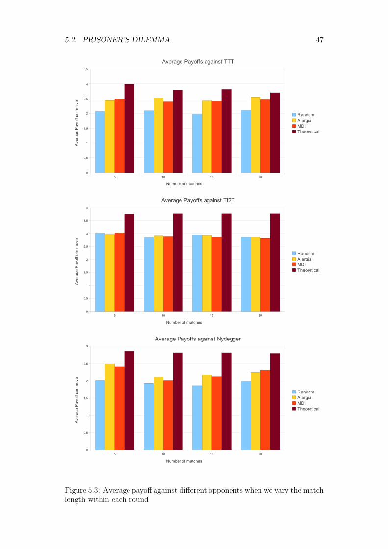
5.2.2 Match length

Here we study how the match length affects our game results in the competi-tion. Remember that match length relates to the length of the words the agentis learning and in turn to the complexity of the prefix tree that the algorithmmust manipulate.

Again the game consists on conducting 500 movements and fixing the num-ber of rounds to 5. Results can be seen in Figure 5.3. This time the result area little bit different than when varying the number of rounds. The differencesbetween the ALERGIA and MDI algorithm seems lesser when only varyingthe match length. Even from the results it could be inferred that the MDIalgorithm is a little bit worse than its competitor. On the other hand, we cansee that changing the match length does not solve the structural problem withthe Tf2T opponent.

5.2.3 Alpha

For this experiment we study the effect of the α parameter on each of thealgorithms. Remember from Sections 3.4.3 and 3.4.4 that the α parametercontrols how liberally could we consider the merge of different states. Loweralphas tend two create automata with less states while increasing the valueallows the addition of more states in the resulting automaton.

Results can be seen in Figure 5.4. It can be seen that when varying α, bestresults are obtained both for low and high values of the parameter. Automatawith a low number of states are somehow “averaging” the symbol frequen-cies because there are few states that can introduce discontinuities in the rateof appearance. On the other hand automata with a high number of statestend to mimic better the structure of the opponent and thus offer better re-sults. So there is a middle range of α values that begin to create structure in

5.2. PRISONER’S DILEMMA 47

Figure 5.3: Average payoff against different opponents when we vary the matchlength within each round


the automata but with diverging results from the ones truly representing theopponent.

5.3 RoShamBo

For the automata in Section 5.2 we had some examples of real automata witha meaningful behaviour in the competition. In this section we are going tostudy how the methodology compares when automata are created randomly.To that end we have created 4 different automata with a random procedure thatpicks at random both the structure (the transitions) and the emitting symbolprobabilities. The chosen game for these experiments will be the RoShamBo(see sec. 2.3.1) that introduces three symbols to pick from and a zero-sumstructure of the rewards. In Appendix B is represented the structure of theautomata. The emitting probabilities have been kept apart in order to improvelegibility.

5.3.1 The experiment

The experiment consists on creating a game composed of 10 rounds with 20matches per round and 10 moves per match, adding up to 2000 moves pergame. Figure 5.3.1 show the results of our learning agent when confrontingto the 2-state and 5-state RoShamBo opponents. For the 2-state opponent,both learning algorithms score below the random opponent (depicted as theinverted triangles in the figure) and when the alpha parameter goes beyonda threshold the learned automata acquires enough complexity and performsalmost optimally. For the 5-state automaton, both algorithms can not reachnear optimal performance despite whichever α we use for training. Howeverthe performance is always better than choosing randomly actions, so some kindof learning has taken place in the learning environment.

Figure 5.3.1 shows the results against the 10-state and 20-state RoShamBoopponents. Again our learning agents behave better than the random oppo-nent with the only noticing particularity that in the 10-state games, the MDIalgorithm performs near optimally for low alpha values, then the performancedrops below the random level for middle values, and regains for higher values.

Another interesting property is that the experiments present a propertyworth mentioning. The complexity of the learned automata scales slowly inthe case of the MDI agent and grows rapidly in the case of the ALERGIAalgorithm.

5.3. ROSHAMBO 49

Figure 5.4: Average payoff against different opponents when we vary the alphaparameter


Figure 5.5: Results against the 2-state and 5-state RoShamBo opponents

5.3. ROSHAMBO 51

Figure 5.6: Results against the 10-state and 20-state RoShamBo opponents

Chapter 6

Conclusions

In this Master’s Thesis we have explored a novel technique to learn agentbehaviour in a competitive environment where Reinforcement Learning pro-cedures are used routinely. The main tool employed in that task has beenthe algorithms for learning probabilistic finite state automata ALERGIA andMDI.

The range of opponents that our agents could learn were constrained tothe class of Stochastic Moore Machines, finite automata that are deterministicin their transitions but that have probabilities associated to the symbols thatthey emit when the automata lands in one of the states.

However, the algorithms before mentioned learn PDFA not transducerslike the Moore Machine. In this thesis we have used the GIATI algorithmframework and extended its usage beyond the N-gram techniques where it wasinitially tested. With this algorithm we can perform translations forward andbackward between an extended language and the pairs of input-output symbolscharacteristic of the transducers.

Once we had our working hypothesis about the Moore Machine that ouropponent holds, we must devise the best strategy to outperform that policy. Inorder to accomplish this task we presented the necessary operations to convertfrom a Mealy Machine to a Markov Decision Process. When the conversioncompletes, we use well known algorithms to devise the best strategy for eachstate.

In order to test our ideas, we developed a game infrastructure where differ-ent players could interact with each other and gathered results on the gamesplayed. Results were very promising since we obtained consistently better re-sults than the random strategy. The random strategy is the best strategy inthese games when the player is uninformed about the opponent strategy, sogetting an advantage over the purely random move generation shows that wewere in the right track.

53

54 CHAPTER 6. CONCLUSIONS

6.1 Future work

The work done in this thesis ranged among several topics (learning PDFAs,transducers, opponent modelling, Markov Decision Processes, etc. . . ) thatcould not be explored in full detail given the time constrains of a Master’sThesis. So picking one of the topics and performing a full research on themcould be very insightful. In particular these are some research lines that couldbe followed in the future:

• Strategy exploration. In this thesis, when exploring the opponentstrategy (that is, to walk over all the states and transitions in the un-known Moore Machine) our learning agent could only rely on the movesgenerated randomly in the first round of the game and on the statesand transitions that could be reached with the inferred rules. This couldleave some parts of the Moore Machine (i.e. the opponent’s strategy)unexplored. More research on how to balance the trade off between ex-ploration and exploitation could be tackled in order to infer more efficientopponents.

• Related to the previous point is the fact that the algorithms employedwhen learning the PDFA do not take into account the payoff matrix

of each of the games. For instance, when faced with how to order statesof the Prefix Tree Acceptor, the algorithms rely on the lexicographicalheuristic. This is a valid heuristic but much more value could be obtainedif that heuristic was related to the payoff matrix and the merging of statescould take this into account.

• In the game structure that we presented in this thesis, games and matchesare preset to a fixed number of moves. Although this could be reasonablein this experimental sandbox it could not make sense in real world envi-ronments. For instance, imagine that the behaviour of a user in a websiteis the opponent we are trying to model with our technology. Clearly theactions that this user performs, can not be constrained to a fixed sizeand they will vary in time. Allowing variable match lengths andhow this affects performance is a valid research extension.

• Once the agent forms the hypothesis about the opposing agent, it runsfreely and does not take into account the symbols that the agent is spit-ting in response to their actions until the next learning round. A verypromising venue of research could be to extend the rules governing theinferred automaton in order to take into account the symbols emittedby the opposing agent. This could lower the uncertainty that we haveabout in which state the Moore Machine currently is and take advantageof it. Extend this thesis using techniques employed learning Partially

Observable Markov Decision Processes .

6.1. FUTURE WORK 55

• Compare the results of this thesis with the results obtained using Rein-forcement Learning techniques

• Extending whichever of the decisions that were taken when deciding thecourse of the thesis. For instance, how other algorithms for learningPDFAs behave in this setup, other policies and parameters for learningthe Markov Decision Processes, extending the range of models that couldrepresent an opponent beyond the Moore Machine, etc. . .

56 CHAPTER 6. CONCLUSIONS

Appendix A

JSON format for a game

Games are specified using the JSON data [Cro]

{

"exp1":{

"player1":{

"type":"ALERGIA",

"alpha":0.7

},

"player2":{

"type":"MOORE_MACHINE",

"filename":"../resources/prisonerMooreMachine.automata"

},

"game":{

"type":"PRISONER",

"numRounds":2,

"numMatchesRound":5,

"matchLength":5

}

}

}

57

58 APPENDIX A. JSON FORMAT FOR A GAME

Appendix B

Automata for the RoShamBo

experiments

0

s

1

r

p

r

sp

Figure B.1: 2-state automata employed in the RoShamBo Experiments

59

60 APPENDIX B. AUTOMATA FOR THE ROSHAMBO EXPERIMENTS

0

ps 2

r

1

r

3

sp

r

p

4s

p

rs

p

sr


0

6

r

7

p

5

s

4r

1p

3s

p 2r

s

s

p

8

r

s

9r

p

p

rs

r

p

s

r

p

s

s

p

r

r

p

s


61

0

1 2

r

2

p

1 6

s

6

1 5

r

s

1 0

p

1r

1 4

s

5

p

1 7

r

1 1

s

p

s

r

8

p

1 9

p

s

4

r

r

7

p

9

s

1 8

p

s

r

p

3

s

r

p

r

s

p

r

s

r

s

p

p

s

r

r

p

s

s

p

r

s

rp

p

r

s

p

s

1 3

r

r

p

sr

s

p


62 APPENDIX B. AUTOMATA FOR THE ROSHAMBO EXPERIMENTS

Bibliography

[ASMO97] Manuel Alfonseca, Justo Sancho, and Miguel Martınez-Orga.Teorıa de lenguajes, gramaticas y automatas. R.A.E.C., 1997.

[Axe84] Robert Axelrod. The Evolution of Cooperation. Basic Books, NewYork, 1984.

[Ber95] Dimitri P. Bertsekas. Dynamic Programming and Optimal Control.Athena Scientific, 1995.

[Ber09] Jean Berstel. Transduction and Context-Free Languages. Teubner-Verlag, 2009.

[BT96] Dimitri P. Bertsekas and John N. Tsitsiklis. Neuro-dynamic pro-gramming, volume 3 of Optimization and Neural Computation Se-ries. Athena Scientific, 1996.

[CM96a] David Carmel and Shaul Markovitch. Learning models of intelli-gent agents. In Proceedings of the Thirteenth National Conferenceon Artificial Intelligence, pages 62–67. AAAI Press, 1996.

[CM96b] David Carmel and Shaul Markovitch. Opponent modeling in multi-agent systems. In Gerhard Weiss and Sandip Sen, editors, Adap-tion And Learning In Multi-Agent Systems, volume 1042 of LectureNotes in Artificial Intelligence. Springer-Verlag, 1996.

[CM98] David Carmel and Shaul Markovitch. Model-based learning of in-teraction strategies in multi-agent systems. Journal of Experimen-tal and Theoretical Artificial Intelligence, 10(3):309–332, 1998.

[CM99] David Carmel and Shaul Markovitch. Exploration strategies formodel-based learning in multiagent systems. Autonomous Agentsand Multi-agent Systems, 2(2):141–172, 1999.

[CO94] Rafael C. Carrasco and Jose Oncina. Learning stochastic regu-lar grammars by means of a state merging method. In Rafael C.Carrasco and Jose Oncina, editors, Proceedings of the Second In-ternational Colloqium on Grammatical Inference and Applications(ICGI94), volume 862 of Lecture Notes in Artificial Intelligence,pages 139–152, Berlin, September 1994. Springer Verlag.

63

64 BIBLIOGRAPHY

[Cro] Douglas Crockford. Json specification website.http://www.json.org.

[CV04] Francisco Casacuberta and Enrique Vidal. Machine translationwith inferred stochastic finite-state transducers. Comput. Linguist.,30(2):205–225, 2004.

[CVP05] Casacuberta, Vidal, and Pico. Inference of finite-state transducersfrom regular languages. PATREC: Pattern Recognition, PergamonPress, 38, 2005.

[Hay08] Simon Haykin. Neural Networks and Learning Machines. PrenticeHall, 3rd edition edition, 2008.

[HMU01] John E. Hopcroft, Rajeev Motwani, and Jeffrey D. Ullman. Intro-duction to automata theory, languages, and computation. AddisonWesley, 2001.

[LR57] R. Duncan Luce and Howard Raiffa. Games and Decisions: Intro-duction and Critical Survey. Dover Publications, 1957.

[Onc92] P. Oncina, J.; Garcıa. Identifying regular languages in polynomialtime, chapter -. World Scientific Publishing, 1992.

[Put94] Martin L. Puterman. Markov decision processes: discrete stochas-tic dynamic programming. John Wiley & Sons, 1994.

[PW04] Lin Padgham and Michael Winikoff. Developing Agent Systems: APractical Guide. Series in Agent Technology. Wiley, 2004.

[RN03] Stuart Russell and Peter Norvig. Artificial Intelligence: A ModernApproach. Prentice-Hall, Englewood Cliffs, NJ, 2nd edition edition,2003.

[SB98] Richard S. Sutton and Andrew G. Barto. Reinforcement Learning:An Introduction (Adaptive Computation and Machine Learning).The MIT Press, March 1998.

[Skl99] David Sklansky. The Theory of Poker. Two plus Two Publishing,1999.

[Tho00] Franck Thollard Thollard. Probabilistic dfa inference usingkullback-leibler divergence and minimality. In In Seventeenth In-ternational Conference on Machine Learning, pages 975–982. Mor-gan Kauffman, 2000.

[Woo02] Michael Wooldridge. An Introduction to MultiAgent Systems. JohnWiley & Sons, 1st edition, June 2002.

http://www.json.org

learning probabilistic finite state automata for opponent ... · master in artificial intelligence...

Documents