learning modules for computational systems biology€¦ · · 2009-02-01learning modules for...

Learning Modules for Computational Systems BiologyLearning Modules for Computational Systems Biology The main features of BioSym™The main features of BioSym

BioSym™ is an interactive, blended learning bio-modeling training course. • BioSym™ addresses important questions relevant to the emerging field of Systems Biology • Real life data are used for model building • The modular structure allows one to incorporate individual models into science curricula at

institutions with different needs • It is of interest to institutions that do not have the full competence to offer courses in Computational

Systems Biology • The concept is based on tested didactical scenarios • Experienced teachers, scientists and e-learning experts, are involved in teaching BioSym™ courses • It incorporates webbased training, team work and e-collaboration • It promotes time independent active participation (distance learning) • It offers links to data bases relevant for modeling topics • BioSym™ is based on widely used mathematical software packages • It makes use of OLAT for the organization of courses • Lectures can be streamed with specialized lecture recording software and presented in OLAT • BioSym™ contains modules which can be used in basic as well as in advanced courses • Learners acquire skills which make BioSym™ useful for “marketable” professional advancement • New contents can be added at any time which assures sustainable usability for a long period of time Examples from BioSymExamples from BioSym Poster presentations by members of the BioSym™ group • BioSym™ - A Systems Biology Learning Network • A computational modeling approach to systems biology • Analysis of complex biological systems through computational mathematical modeling • Bio-Thermodynamics: Understanding glycolysis with quantum chemistry • Modeling of metabolic networks: A computational approach to functional systems biochemistry and

metabolic engineering • Selection and adaptation in microbial communities: A computational modeling approach to

ecosystem complexity • Eco-genomics of rumen communities: How similar, in an evolutionary sense, are cellulases from

different rumen microbes? Kurt Hanselmann ([email protected]), Christoph Fuchs ([email protected]), Stefan Schafroth ([email protected]), Maja A. Lazzaretti-Ulmer ([email protected]), Roman Kälin ([email protected]), Stefan Brammertz ([email protected]), Hans Ulrich Suter ([email protected]) BioSym™ - Computational Systems Biology [email protected] or [email protected]

** Network Partners** Network Partners: University Zurich, ETH Zurich, ZH Winterthur, University Fribourg, Ruhr University Bochum, WHO Geneva, Roche Basel, UniversityHospital Basel. Collaborators UZH: Collaborators UZH: Barbour Andrew D. math., Brammertz Stefan biol., Fuchs Christoph1 inform., Hanselmann Kurt2 biol., HeinzmannDominik math., Kälin Roman math., Lazzaretti Maja biol., Schafroth Stefan phys., Suter Hans Ulrich chem. 1 [email protected], 2 [email protected]

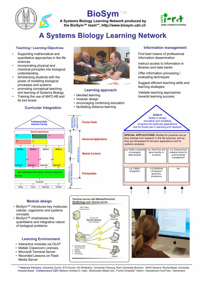
A Systems Biology Learning NetworkA Systems Biology Learning Network

BioSym™BioSymA Systems Biology Learning Network produced by

the BioSym™ team**, http;//www.biosym.uzh.ch

Curricular IntegrationCurricular Integration

Learning EnvironmentLearning Environment• Interactive modules via OLAT• Matlab Classroom Licenses• Microsoft Terminal Server• Recorded Lessons on Flash

Media Server

Information managementInformation managementFind best means of professionalinformation dissemination

Instruct access to information inlibraries and data banks

Offer information processing /evaluating techniques

Suggest efficient teaching skills andlearning strategies

Validate teaching approachestowards learning success

Teaching / Learning ObjectivesTeaching / Learning Objectives

• Supporting mathematical andquantitative approaches in the lifesciences

• incorporating physical andchemical principles into biologicalunderstanding

• familiarizing students with thepower of modeling biologicalprocesses and systems

• promoting conceptual teachingand learning of Systems Biology

• Training the use of MATLAB andits tool boxes

Learning approachLearning approach• blended learning• modular design• encouraging continuing education• facilitating distance learning

Module designModule design• BioSym™ introduces key molecular,

cellular, organismic and systemsconcepts

• BioSym™ emphasizes thequantitative and integrative natureof biological problems

SPECIAL APPLICATIONS: Models for practical use asthey emerge from research in the life sciences, and asthey are developed for bio-tech applications and forsystems analyses.

e.g. Pattern analysesof ecologicaldeterminants

e.g. Gene flux andgene transfer in

evolution

e.g. Energy fluxesmaterial cycles for

environmentalmanagement

e.g. Patternrecognition

e.g.Statisticalcomparisongenomics,proteomics

GOALSAbility to design

simulation and modellingprograms for particular applications

and for broad use in teaching and research.

etc.

A computational modeling approach to systems biology Christoph Fuchs ([email protected]) and Kurt Hanselmann ([email protected]), BioSym™ - Computational Systems Biology, Institute of Mathematics, University of Zürich, Winterthurerstr. 190, 8057 Zürich Today it has become essential to employ mathematical models as research tools at all levels of biology. BioSym is a compilation of interactive models which can be used to study biological systems quantitatively, from the molecular to the ecosystem level. The models are based on biological and physicochemical principles which can be expressed with mathematical algorithms. They are offered under http://www.biosym.unizh.ch/index.php. BioSym contains classical deterministic models and more complex stochastic ones (e.g. epidemics, metabolic networks, gene regulation and metabolic control, physiology, gene/protein evolution etc.). On an advanced level, it introduces models which can assist users in designing quantitative experiments with proper boundary conditions and handling large data sets. Systems biology with BioSym is a logical step towards synthesizing details and fragments of knowledge into a more holistic view of biology, and it can serve as a motivation to deal with the complexity inherent to many biological systems. Courses which are offered by the BioSym team introduce users to model building, show them how to design mathematical models and train them how to use simulations. The learning modules are primarily based on MATLAB and its toolboxes. Many models contain a Java Applet or a Flash animation to illustrate the details of the background.

BioSym™BioSym™

BioSym™

BioSym™

BioSym™

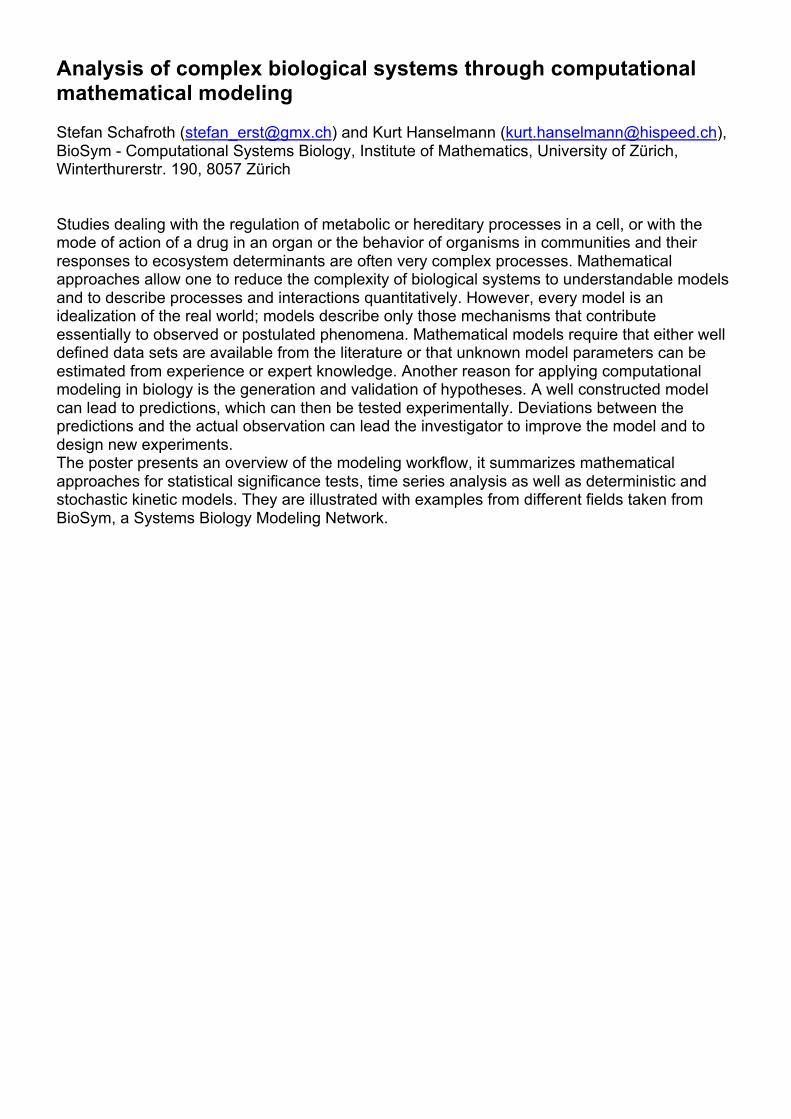
Analysis of complex biological systems through computational mathematical modeling Stefan Schafroth ([email protected]) and Kurt Hanselmann ([email protected]), BioSym - Computational Systems Biology, Institute of Mathematics, University of Zürich, Winterthurerstr. 190, 8057 Zürich Studies dealing with the regulation of metabolic or hereditary processes in a cell, or with the mode of action of a drug in an organ or the behavior of organisms in communities and their responses to ecosystem determinants are often very complex processes. Mathematical approaches allow one to reduce the complexity of biological systems to understandable models and to describe processes and interactions quantitatively. However, every model is an idealization of the real world; models describe only those mechanisms that contribute essentially to observed or postulated phenomena. Mathematical models require that either well defined data sets are available from the literature or that unknown model parameters can be estimated from experience or expert knowledge. Another reason for applying computational modeling in biology is the generation and validation of hypotheses. A well constructed model can lead to predictions, which can then be tested experimentally. Deviations between the predictions and the actual observation can lead the investigator to improve the model and to design new experiments. The poster presents an overview of the modeling workflow, it summarizes mathematical approaches for statistical significance tests, time series analysis as well as deterministic and stochastic kinetic models. They are illustrated with examples from different fields taken from BioSym, a Systems Biology Modeling Network.

** Network Partners** Network Partners: University Zurich, ETH Zurich, ZH Winterthur, University Fribourg, Ruhr University Bochum, WHO Geneva, Roche Basel,University Hospital Basel. Collaborators UZH: Collaborators UZH: Barbour Andrew D. math., Brammertz Stefan biol., Fuchs Christoph1 inform., Hanselmann Kurt2 biol.,Heinzmann Dominik math., Kälin Roman math., Lazzaretti Maja biol., Schafroth Stefan phys., Suter Hans Ulrich chem. 1 [email protected], 2 [email protected]

Mathematical Mathematical modelingmodelingin biology: 3 good reasonsin biology: 3 good reasons

• Managing complexity and handlinguncertainty: A model is always anidealization of the real world using only welldefined input data.

• Modeling requires abstraction: The modeldescribes only those underlyingmechanisms that contribute most strongly tothe observed phenomenon.This results in areduction of complexity.

• Generation and validation of hypotheses:A good model can produce observablepredictions. Deviations of predictions fromactual observations can lead to modelimprovement.

Models Models can illustrate can illustrate simplesimplerelationshipsrelationships

Example: How bacteria consumesubstrates. Application of a rate flowmodel.

The use of deterministic andThe use of deterministic andstochastic algorithmsstochastic algorithms

Basic techniques for time seriesBasic techniques for time seriesanalysisanalysis

Time series data often arise whenmonitoring physical processes. Timeseries analysis accounts for the fact thatdata points taken over time may have aninternal structure (such as auto-correlation, trend or seasonal variation)that should be accounted for.

Exponential smoothingExponential smoothing assignsexponentially decreasing weights asthe observations get older. This is incontrast to single moving averageswhere past observations are weighedequally. Exponential smoothing is avery popular scheme to produce asmoothed time series.

Double exponential smoothing usestwo constants and is better at handlingtrends.

Simple models can showSimple models can showcomplex behaviourcomplex behaviour

In 1976 the Australian theoretical ecologistRobert May showed that simple first orderdifference equations can have very complicatedor even unpredictable dynamics. The LogisticDifference Equation (LDE) is a model to explorethe route into chaotic behaviour. The route tochaos starts with period doublings.

LDE: Stable cycles with period k. The red linerepresents the trajectory (time course) of thesystem in the phase plane.

In the refinement process these stages arerepeatedly executed in a virtually never-ending process which generates models ofincreasing generality and validity.

Conceptualization

Formulation

Numerical

Implementation

Computation

Validation

Refinement

Start End

0 5 10 15 20 25 3018

18.2

18.4

18.6

18.8

19

19.2

19.4

19.6

19.8

20

Time (days)

Water temperature (degrees C)

Moving averages of different sizes

Original data

Moving average of size 2




0 5 10 15 20 25 30 35 40-1.5

-1

-0.5

0

0.5

1

1.5

2

Time (days)


Single exponential smoothing

Original data

alpha=0.1, mse=0.43159

alpha=0.5, mse=0.25079

alpha=0.9, mse=0.31097

0 5 10 15 20 25 30 35 40-1.5

-1

-0.5

0

0.5

1

1.5

2

2.5

3

Time (days)


Double exponential smoothing

Original data

alpha=0.10, gamma=0.94, mse=0.74108

alpha=0.27, gamma=0.94, mse=0.28063

alpha=0.80, gamma=0.94, mse=0.56122

0 20 40 60 80 100 120 140 160 180 2000

100

200

300

400

500

600

700

800

900

1000

Time [s]

Number of molecules

Deterministic and stochastic model (Stochastic Petri Net)

r(t) determ

r2(t) determ

r(t) stoch

r2(t) stoch

3 3.1 3.2 3.3 3.4 3.5 3.6 3.7 3.8 3.9 40

0.1

0.2

0.3

0.4

0.5

0.6

0.7

0.8

0.9

1

Analysis of Complex Biological SystemsAnalysis of Complex Biological Systems

A A modeling modeling workflow consists ofworkflow consists offive stagesfive stages

C external nutrientsX0 unoccupied receptorX1 occupied receptorP internal nutrientsX0+X1 = constant

dC/dt = -k1C*X0 + k-1X1dX0/dt = -k1C*X0 + k-1X1+ k2X1dX1/dt =k1C*X0 - k-1X1- k2X1dP/dt = k2X1

C + X

0

k1! "! X1 ; X

1

k#1! "! C + X

0 ; X

1

k2! "! P + Xo

C and X0 can combine to form the complex X1

BioSymBioSym™™A Systems Biology Learning Network produced by


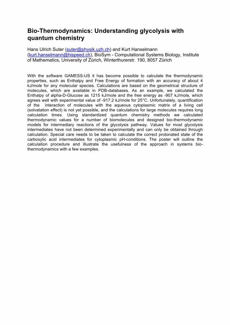
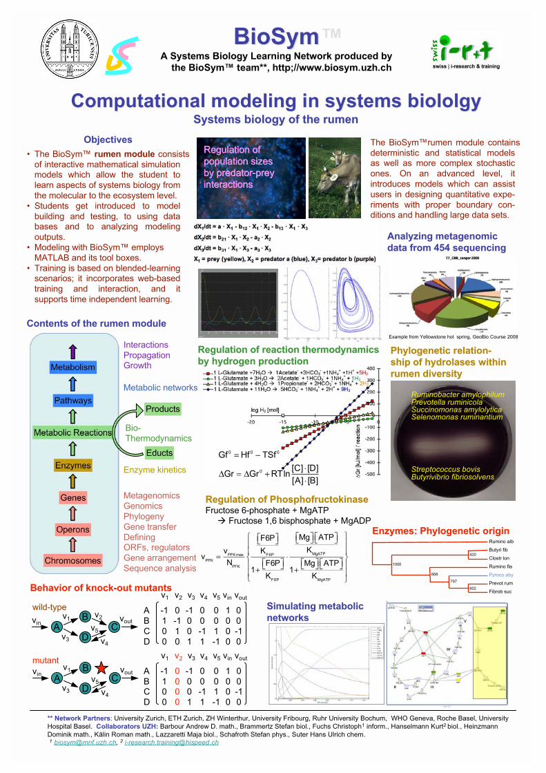
Bio-Thermodynamics: Understanding glycolysis with quantum chemistry Hans Ulrich Suter ([email protected]) and Kurt Hanselmann ([email protected]), BioSym - Computational Systems Biology, Institute of Mathematics, University of Zürich, Winterthurerstr. 190, 8057 Zürich With the software GAMESS-US it has become possible to calculate the thermodynamic properties, such as Enthalpy and Free Energy of formation with an accuracy of about 4 kJ/mole for any molecular species. Calculations are based on the geometrical structure of molecules, which are available in PDB-databases. As an example, we calculated the Enthalpy of alpha-D-Glucose as 1215 kJ/mole and the free energy as -907 kJ/mole, which agrees well with experimental value of -917.2 kJ/mole for 25°C. Unfortunately, quantification of the interaction of molecules with the aqueous cytoplasmic matrix of a living cell (solvatation effect) is not yet possible, and the calculations for large molecules requires long calculation times. Using standardized quantum chemistry methods we calculated thermodynamic values for a number of biomolecules and designed bio-thermodynamic models for intermediary reactions of the glycolysis pathway. Values for most glycolysis intermediates have not been determined experimentally and can only be obtained through calculation. Special care needs to be taken to calculate the correct protonated state of the carboxylic acid intermediates for cytoplasmic pH-conditions. The poster will outline the calculation procedure and illustrate the usefulness of the approach in systems bio-thermodynamics with a few examples.

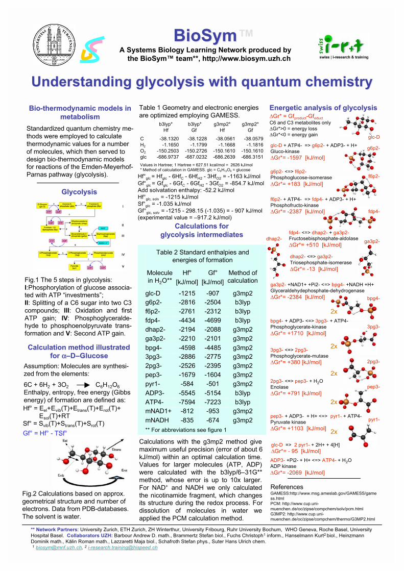
Bio-thermodynamic models inBio-thermodynamic models in

metabolismmetabolism

GlycolysisGlycolysis

Energetic analysis of Energetic analysis of glycolysisglycolysis

Understanding Understanding glycolysis glycolysis with quantum chemistrywith quantum chemistry

Fig.1 The 5 steps in glycolysis:

I:Phosphorylation of glucose associa-ted with ATP “investments”;

II: Splitting of a C6 sugar into two C3

compounds; III: Oxidation and first

ATP gain; IV: Phosphoglyceralde-hyde to phosphoenolpyruvate trans-

formation and V: Second ATP gain.

Calculations forCalculations for

glycolysis glycolysis intermediatesintermediates

** Network Partners** Network Partners: University Zurich, ETH Zurich, ZH Winterthur, University Fribourg, Ruhr University Bochum, WHO Geneva, Roche Basel, University

Hospital Basel. Collaborators UZH: Collaborators UZH: Barbour Andrew D. math., Brammertz Stefan biol., Fuchs Christoph1 inform., Hanselmann Kurt2 biol., Heinzmann

Dominik math., Kälin Roman math., Lazzaretti Maja biol., Schafroth Stefan phys., Suter Hans Ulrich chem.

1 [email protected], 2 [email protected]

Table 1 Geometry and electronic energies

are optimized employing GAMESS.

Standardized quantum chemistry me-

thods were employed to calculate

thermodynamic values for a number

of molecules, which then served to

design bio-thermodynamic modelsfor reactions of the Emden-Meyerhof-

Parnas pathway (glycolysis).

Calculations with the g3mp2 method give

maximum useful precision (error of about 6

kJ/mol) within an optimal calculation time.Values for larger molecules (ATP, ADP)

were calculated with the b3lyp/6–31G**

method, whose error is up to 10x larger.

For NAD+ and NADH we only calculated

the nicotinamide fragment, which changesits structure during the redox process. For

dissolution of molecules in water we

applied the PCM calculation method.

Assumption: Molecules are synthesi-

zed from the elements:

6C + 6H2 + 3O2 C6H12O6

Enthalpy, entropy, free energy (Gibbs

energy) of formation are defined as:

Hf° = Eel+Evib(T)+Etrans(T)+Erot(T)+

Esol(T)+RTSf° = Svib(T)+Strans(T)+Srot(T)

Calculation method illustratedCalculation method illustrated

forfor ––DD––GlucoseGlucose

Hf°glc = Hfglc - 6HfC - 6HfH2 - 3HfO2 = -1163 kJ/mol

Gf°glc = Gfglc - 6GfC - 6GfH2 - 3GfO2 = -854.7 kJ/mol

Add solvatation enthalpy: -52.2 kJ/mol

Hf°glc, solv = -1215 kJ/mol

Sf°glc = -1.035 kJ/mol

Gf°glc, solv = -1215 - 298.15 (-1.035) = - 907 kJ/mol

(experimental value = –917.2 kJ/mol)

b3lyp* b3lyp* g3mp2* g3mp2*

Hf Gf Hf Gf

C -38.1320 -38.1228 -38.0561 -38.0579

H2 -1.1650 -1.1799 -1.1668 -1.1816

O2 -150.2503 -150.2726 -150.1610 -150.1610

glc -686.9737 -687.0232 -686.2639 -686.3151

Values in Hartree; 1 Hartree = 627.51 kcal/mol = 2626 kJ/mol

* Method of calculation in GAMESS. glc = C6H12O6 = glucose

Gf° = Hf° - TSf°

Fig.2 Calculations based on approx.

geometrical structure and number ofelectrons. Data from PDB-databases.

The solvent is water.

** For abbreviations see figure 1

Table 2 Standard enthalpies and

energies of formation

g3mp2-674-835mNADH

g3mp2-953-812mNAD1+

b3lyp-7223-7594ATP4-

b3lyp-5154-5545ADP3-

g3mp2-501-584pyr1-

g3mp2-1604-1679pep3-

g3mp2-2395-25262pg3-

g3mp2-2775-28863pg3-

g3mp2-4485-4598bpg4-

g3mp2-2101-2210ga3p2-

g3mp2-2088-2194dhap2-

b3lyp-4699-4434fdp4-

b3lyp-2312-2761f6p2-

b3lyp-2504-2816g6p2-

g3mp2-907-1215glc-D

Method of

calculation

Gf°

[kJ/mol]

Hf°

[kJ/mol]

Molecule

in H2O**

ReferencesGAMESS:http://www.msg.ameslab.gov/GAMESS/game

ss.html

PCM: http://www.cup.uni-

muenchen.de/oc/zipse/compchem/solv/pcm.html

G3MP2: http://www.cup.uni-

muenchen.de/oc/zipse/compchem/thermo/G3MP2.html

ga3p2- +NAD1+ +Pi2- <=> bpg4- +NADH +H+

Glyceraldehydephosphate-dehydrogenase

Gr*= -2384 [kJ/mol]

3pg3- <=> 2pg3-

Phosphoglycerate-mutase

Gr*= +380 [kJ/mol]

2pg3- <=> pep3- + H2O

Enolase

Gr*= +791 [kJ/mol]

pep3- + ADP3- + H+ <=> pyr1- + ATP4-

Pyruvate kinase

Gr*= +1103 [kJ/mol]

glc-D + ATP4- => g6p2- + ADP3- + H+

Gluco-kinase

Gr*= -1597 [kJ/mol]

2x

2x

2x

2x

2x

f6p2- + ATP4- => fdp4- + ADP3- + H+

Phosphofructo-kinase

Gr*= -2387 [kJ/mol]

g6p2- <=> f6p2-

Phosphoglucose-isomerase

Gr*= +183 [kJ/mol]

fdp4- <=> dhap2- + ga3p2-Fructosebisphosphate-aldolase

Gr*= +510 [kJ/mol]

dhap2- <=> ga3p2-

Triosephosphate-isomerase

Gr*= -13 [kJ/mol]

Gr* = Gfproduct-Gfeduct

C6 and C3 metabolites only

Gr*>0 = energy loss

Gr*<0 = energy gain

ADP3- +Pi2- + H+ <=> ATP4- + H2O

ADP kinase

Gr*= -2069 [kJ/mol]

g6p2-

f6p2-

fdp4-

ga3p2-dhap2-

bpg4-

3pg3-

2pg3-

pep3-

pyr1-

glc-D

bpg4- + ADP3- <=> 3pg3- + ATP4-

Phosphoglycerate-kinase

Gr*= +1710 [kJ/mol]

glc-D => 2 pyr1- + 2H+ + 4[H]

Gr*= - 95 [kJ/mol]



Modeling of metabolic networks: A computational approach to functional systems biochemistry and metabolic engineering Stefan Brammertz ([email protected]) and Kurt Hanselmann ([email protected]), BioSym - Computational Systems Biology, Institute of Mathematics, University of Zürich, Winterthurerstr. 190, 8057 Zürich The biochemistry of individual reactions in the Embden-Meyerhof-Parnas pathway (glycolysis), the Krebs cycle (citric acid cycle) and the Calvin-Benson cycle (pentose phosphate pathway) are well established. These three pathways and a number of related ones play key roles in cellular processes of many aerobic and anaerobic, prokaryotic and eukaryotic organisms. We made an attempt to design mathematical models for the quantitative analysis and dynamic simulation of these pathways. The models are based on Michaelis-Menten rate equations and mass transfer concepts; the software Simbiology (The Mathworks) is employed for model design. The models allow one to study interactions between different processes with linked biochemical reactions, the regulation of enzymes and process optimization. Enzyme parameters (Km, Ki, vmax, etc.) and concentrations of metabolites are compiled from different databases available on the www (BRENDA, KEGG, ExPASy, etc.) and from scientific publications. The values are then screened for reliability and missing values are chosen based on expert knowledge. Dynamic models are excellent learning and research tools because they allow one to study the role of individual enzymes within complex cellular metabolic networks which may lead to new hypotheses. Numerous options can be tested in silico before one designs and carries out experiments in vivo or in vitro.

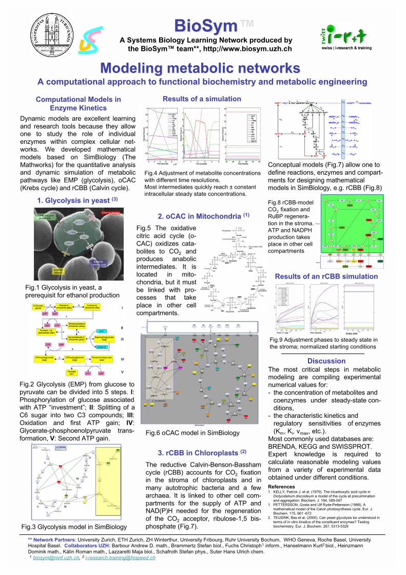
Computational Models inComputational Models in

Enzyme KineticsEnzyme Kinetics

Dynamic models are excellent learning

and research tools because they allowone to study the role of individual

enzymes within complex cellular net-

works. We developed mathematical

models based on SimBiology (The

Mathworks) for the quantitative analysisand dynamic simulation of metabolic

pathways like EMP (glycolysis), oCAC

(Krebs cycle) and rCBB (Calvin cycle).

2. 2. oCACoCAC in in MitochondriaMitochondria (1)(1)

1. 1. Glycolysis Glycolysis in yeast in yeast (3)(3)

DiscussionDiscussion

Fig.3 Glycolysis model in SimBiology

Fig.1 Glycolysis in yeast, a

prerequisit for ethanol production

Conceptual models (Fig.7) allow one to

define reactions, enzymes and compart-

ments for designing mathematicalmodels in SimBiology, e.g. rCBB (Fig.8)

Fig.4 Adjustment of metabolite concentrations

with different time resolutions.

Most intermediates quickly reach ± constant

intracellular steady state concentrations.

References1. KELLY, Patrick J. et al. (1979). The tricarboxylic acid cycle in

Dictyostelium discoideum a model of the cycle at preculmination

and aggregation. Biochem. J. 184, 589-597

1. PETTERSSON, Gosta and Ulf Ryde-Pettersson (1988). A

mathematical model of the Calvin photosynthesis cycle. Eur. J.

Biochem. 175, 661 -672

2. TEUSINK, Bas et al. (2000). Can yeast glycolysis be understood in

terms of in vitro kinetics of the constituent enzymes? Testing

biochemistry. Eur. J. Biochem. 267, 5313-5329

Modeling metabolic networksModeling metabolic networks A computational approach to functional biochemistry and metabolic engineeringA computational approach to functional biochemistry and metabolic engineering

Fig.2 Glycolysis (EMP) from glucose to

pyruvate can be divided into 5 steps. I:

Phosphorylation of glucose associatedwith ATP “investment”; II: Splitting of a

C6 sugar into two C3 compounds; III:

Oxidation and first ATP gain; IV:

Glycerate-phosphoenolpyruvate trans-

formation, V: Second ATP gain.

Fig.5 The oxidative

citric acid cycle (o-

CAC) oxidizes cata-

bolites to CO2 andproduces anabolic

intermediates. It is

located in mito-

chondria, but it must

be linked with pro-cesses that take

place in other cell

compartments.

Fig.6 oCAC model in SimBiology

Results of a simulationResults of a simulation

The most critical steps in metabolicmodeling are compiling experimental

numerical values for:

- the concentration of metabolites and

coenzymes under steady-state con-

ditions,- the characteristic kinetics and

regulatory sensitivities of enzymes

(Km, Ki, vmax, etc.).

Most commonly used databases are:

BRENDA, KEGG and SWISSPROT.Expert knowledge is required to

calculate reasonable modeling values

from a variety of experimental data

obtained under different conditions.

** Network Partners** Network Partners: University Zurich, ETH Zurich, ZH Winterthur, University Fribourg, Ruhr University Bochum, WHO Geneva, Roche Basel, UniversityHospital Basel. Collaborators UZH: Collaborators UZH: Barbour Andrew D. math., Brammertz Stefan biol., Fuchs Christoph1 inform., Hanselmann Kurt2 biol., Heinzmann



3. 3. rCBB rCBB in Chloroplasts in Chloroplasts (2)(2)

The reductive Calvin-Benson-Bassham

cycle (rCBB) accounts for CO2 fixationin the stroma of chloroplasts and in

many autotrophic bacteria and a few

archaea. It is linked to other cell com-

partments for the supply of ATP andNAD(P)H needed for the regeneration

of the CO2 acceptor, ribulose-1,5 bis-

phosphate (Fig.7).

Fig.8 rCBB-model

CO2 fixation and

RuBP regenera-

tion in the stroma.

ATP and NADPH

production takes

place in other cell

compartments

Fig.9 Adjustment phases to steady state in

the stroma; normalized starting conditions

Results of an Results of an rCBB rCBB simulationsimulation



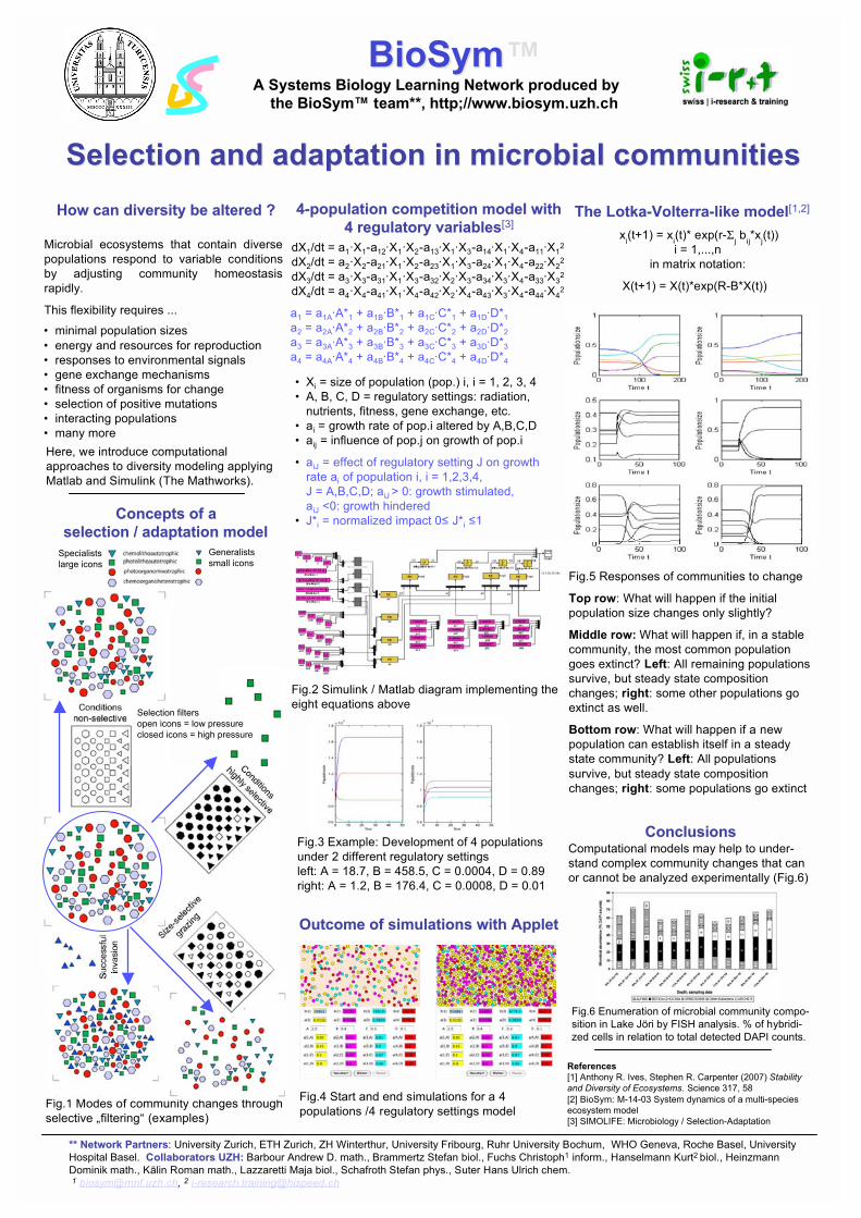
Selection and adaptation in microbial communities: A computational modeling approach to ecosystem complexity Roman Kälin ([email protected]), Munti Yuhana ([email protected]) and Kurt Hanselmann ([email protected]), BioSym - Computational Systems Biology, Institute of Mathematics, University of Zürich, Winterthurerstr. 190, 8057 Zürich Stability and dynamics of an ecosystem depends on the ability of its organisms to interact with each other and to quickly respond to perturbations. We have studied changes in microbial community compositions in a remote high mountain lake that seasonally passes through extremes of environmental changes. The ecosystem was analyzed applying molecular techniques which are based on biomolecular indicators and combined with measurements of physicochemical ecosystem determinants. The diversity of organisms is overwhelming and, due to the variability of parameter combinations under natural conditions, one can seldom observe similar population compositions under seemingly similar environmental settings. Instead, numerous community patterns emerge from the lake’s population pool which allow one to create hypotheses and concepts about the role of selection and adaptation in community regulation. We have developed a computational “selection-adaptation model” based on extended Lotka-Volterra algorithms that allows one to simulate population development and disappearance with predetermined parameter assignments. The investigator can define stabilizing and destabilizing mechanisms and follow population diversity changes. An understanding of ecosystem complexity cannot be reached by observation and experimentation alone. Good theoretical models help one to carry out numerous simulations in silico and to define those environmental determinants and organismic characteristics that might play essential regulatory roles.





How can diversity be altered ?How can diversity be altered ?

Microbial ecosystems that contain diverse

populations respond to variable conditions

by adjusting community homeostasis

rapidly.

This flexibility requires ...

ConclusionsConclusions

The The Lotka-Volterra-like Lotka-Volterra-like modelmodel[1,2]

xi(t+1) = x

i(t)* exp(r-

j b

ij*x

j(t))

i = 1,...,n

in matrix notation:

X(t+1) = X(t)*exp(R-B*X(t))

Fig.3 Example: Development of 4 populations

under 2 different regulatory settings

left: A = 18.7, B = 458.5, C = 0.0004, D = 0.89

right: A = 1.2, B = 176.4, C = 0.0008, D = 0.01

Fig.5 Responses of communities to change

Top row: What will happen if the initial

population size changes only slightly?

Middle row: What will happen if, in a stable

community, the most common population

goes extinct? Left: All remaining populations

survive, but steady state composition

changes; right: some other populations go

extinct as well.

Bottom row: What will happen if a new

population can establish itself in a steady

state community? Left: All populations

survive, but steady state composition

changes; right: some populations go extinct

References

[1] Anthony R. Ives, Stephen R. Carpenter (2007) Stability

and Diversity of Ecosystems. Science 317, 58

[2] BioSym: M-14-03 System dynamics of a multi-species

ecosystem model

[3] SIMOLIFE: Microbiology / Selection-Adaptation

Selection and adaptation in microbial communitiesSelection and adaptation in microbial communities

Fig.2 Simulink / Matlab diagram implementing the

eight equations above

• minimal population sizes

• energy and resources for reproduction

• responses to environmental signals

• gene exchange mechanisms

• fitness of organisms for change

• selection of positive mutations

• interacting populations

• many more

4-population competition model with4-population competition model with

4 regulatory variables4 regulatory variables[3]

a1 = a1A·A*1 + a1B·B*1 + a1C·C*1 + a1D·D*1

a2 = a2A·A*2 + a2B·B*2 + a2C·C*2 + a2D·D*2

a3 = a3A·A*3 + a3B·B*3 + a3C·C*3 + a3D·D*3

a4 = a4A·A*4 + a4B·B*4 + a4C·C*4 + a4D·D*4

Outcome of simulations with AppletOutcome of simulations with Applet

Fig.1 Modes of community changes through

selective „filtering“ (examples)

Fig.4 Start and end simulations for a 4

populations /4 regulatory settings model

Concepts ofConcepts of aa

selection / adaptation modelselection / adaptation model

dX1/dt = a1·X1-a12·X1·X2-a13·X1·X3-a14·X1·X4-a11·X12




Fig.6 Enumeration of microbial community compo-

sition in Lake Jöri by FISH analysis. % of hybridi-

zed cells in relation to total detected DAPI counts.

Computational models may help to under-

stand complex community changes that can

or cannot be analyzed experimentally (Fig.6)

Here, we introduce computational

approaches to diversity modeling applying

Matlab and Simulink (The Mathworks).

• Xi = size of population (pop.) i, i = 1, 2, 3, 4

• A, B, C, D = regulatory settings: radiation,

nutrients, fitness, gene exchange, etc.

• ai = growth rate of pop.i altered by A,B,C,D

• aij = influence of pop.j on growth of pop.i

• aiJ = effect of regulatory setting J on growth

rate ai of population i, i = 1,2,3,4,

J = A,B,C,D; aiJ > 0: growth stimulated,

aiJ <0: growth hindered

• J*i = normalized impact 0 J*i 1



Specialists

large icons

Generalists

small icons

Conditions

non-selective

Conditions

highly selective

Successfu

l

invasio

n

Size-

selective

graz

ing

Selection filters

open icons = low pressure

closed icons = high pressure

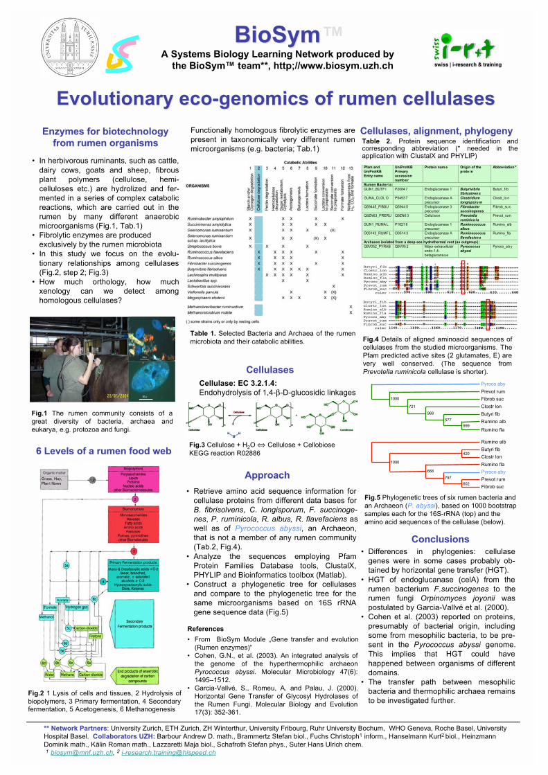
Eco-genomics of rumen communities: How similar, in an evolutionary sense, are cellulases from different rumen microbes? Maja A. Lazzaretti-Ulmer ([email protected]) and Kurt Hanselmann ([email protected]), BioSym - Computational Systems Biology, Institute of Mathematics, University of Zürich, Winterthurerstr. 190, 8057 Zürich The rumen is a complex ecosystem. Its microbiota comprises mostly anaerobic bacteria and archaea, anaerobic, ciliated protozoa and anaerobic fungi. Cellulose (C6H10O5)n is enzymatically hydrolized in a first step by cellulases produced by some members of the microbiota. The resulting di- and monosaccharides are then further utilized by the same and by other microbes of the community, which produce volatile fatty acids, CO2, CH4 and a number of other metabolites. We retrieved amino acid sequence information for cellulase proteins for a number of rumen microorganisms (Butyrivibrio fibrisolvens, Clostridium longisporum, Fibrobacter succinogenes, Prevotella ruminicola, Ruminococcus albus and Ruminococcus flavefaciens) from different data bases as well as of Pyrococcus abyssi, an Archaeon, which is not a member of any rumen community, and compared them employing the Pfam Protein Families Database tools and the softwares ClustalX and PHYLIP. The resulting phylogenetic tree was then compared with the phylogenetic tree made for the same microorganisms based on their 16S rRNA data. The two trees revealed interesting differences, which suggest that cellulase genes were in some cases obtained by horizontal gene transfer. It is surprising that this should have been happened between microorganisms of different domains and the transfer path between mesophilic bacteria and thermophilic archaea remains to be further investigated.

Evolutionary eco-genomics of rumen Evolutionary eco-genomics of rumen cellulasescellulases







ApproachApproach

• Retrieve amino acid sequence information for

cellulase proteins from different data bases for

B. fibrisolvens, C. longisporum, F. succinoge-

nes, P. ruminicola, R. albus, R. flavefaciens as

well as of Pyrococcus abyssi, an Archaeon,

that is not a member of any rumen community

(Tab.2, Fig.4).

• Analyze the sequences employing Pfam

Protein Families Database tools, ClustalX,

PHYLIP and Bioinformatics toolbox (Matlab).

• Construct a phylogenetic tree for cellulases

and compare to the phylogenetic tree for the

same microorganisms based on 16S rRNA

gene sequence data (Fig.5)

Enzymes for biotechnologyEnzymes for biotechnology

from rumen organismsfrom rumen organisms

• In herbivorous ruminants, such as cattle,

dairy cows, goats and sheep, fibrous

plant polymers (cellulose, hemi-

celluloses etc.) are hydrolized and fer-

mented in a series of complex catabolic

reactions, which are carried out in the

rumen by many different anaerobic

microorganisms (Fig.1, Tab.1)

• Fibrolytic enzymes are produced

exclusively by the rumen microbiota

• In this study we focus on the evolu-

tionary relationships among cellulases

(Fig.2, step 2; Fig.3)

• How much orthology, how much

xenology can we detect among

homologous cellulases?

Fig.1 The rumen community consists of a

great diversity of bacteria, archaea and

eukarya, e.g. protozoa and fungi.

CellulasesCellulases

Fig.3 Cellulose + H2O Cellulose + Cellobiose

KEGG reaction R02886

Cellulase: EC 3.2.1.4:

Endohydrolysis of 1,4- -D-glucosidic linkages

ConclusionsConclusions

• Differences in phylogenies: cellulase

genes were in some cases probably ob-

tained by horizontal gene transfer (HGT).

• HGT of endoglucanase (celA) from the

rumen bacterium F.succinogenes to the

rumen fungi Orpinomyces joyonii was

postulated by Garcia-Vallvé et al. (2000).

• Cohen et al. (2003) reported on proteins,

presumably of bacterial origin, including

some from mesophilic bacteria, to be pre-

sent in the Pyrococcus abyssi genome.

This implies that HGT could have

happened between organisms of different

domains.

• The transfer path between mesophilic

bacteria and thermophilic archaea remains

to be investigated further.Fig.2 1 Lysis of cells and tissues, 2 Hydrolysis of

biopolymers, 3 Primary fermentation, 4 Secondaryfermentation, 5 Acetogenesis, 6 Methanogenesis

6 Levels of a rumen food web6 Levels of a rumen food web

Grass, Hay,

Plant fibres

Pfam and

UniProtKB Entry name

UniProtKB

Primary accession

number

Protein nam e Origin of the

prote in Abbreviation *

Rumen Bacteria: GUN1_BUTF I P2084 7 Endoglucanase 1 Butyrivibrio

fibrisolven s Butyri_f ib

GUNA_CLOL O P5493 7 Endoglucanase A

precursor Clostridium

longisporu m Clostr_lo n

Q59445_FIBSU Q5944 5 Endoglucanase 3 precursor

Fibrobacter succinogenes

Fibrob_su c

Q9ZN63_PRERU Q9ZN6 3 Cellulase Prevotella

ruminico la Prevot_rum

GUN1_RUMA L P1621 6 Endoglucanase 1 precursor

Ruminococcus albus

Rumino_alb

O05143_RUMF L O0514 3 Endoglucanase A

precursor Ruminococcus

flavefacien s Rumino_fla

Archaeon isolated from a deep-sea hydrothermal vent (as outgroup) : Q9V052_PYRAB Q9V05 2 Major extracellular

endo-1,4-

betaglucanase

Pyrococcus

abyssi

Pyroco_aby

CellulasesCellulases, alignment, phylogeny, alignment, phylogenyTable 2. Protein sequence identification andcorresponding abbreviation (* needed in theapplication with ClustalX and PHYLIP)

Fig.4 Details of aligned aminoacid sequences of

cellulases from the studied microorganisms. The

Pfam predicted active sites (2 glutamates, E) are

very well conserved. (The sequence from

Prevotella ruminicola cellulase is shorter).

Fig.5 Phylogenetic trees of six rumen bacteria and

an Archaeon (P. abyssi), based on 1000 bootstrap

samples each for the 16S-rRNA (top) and the

amino acid sequences of the cellulase (below).

Rumino alb

Butyri fib

Clostr lon

Rumino fla

Pyroco aby

Prevot rum

Fibrob suc

1000

420

668

797

602

Pyroco aby

Prevot rum

Fibrob suc

Clostr lon

Butyri fib

Rumino alb

1000

721

968

577

999Rumino fla

Butyri_fib Clostr_lon Rumino_alb Rumino_fla Pyroco_aby Prevot_rum Fibrob_suc

ruler

Butyri_fib Clostr_lon Rumino_alb Rumino_fla Pyroco_aby Prevot_rum Fibrob_suc

ruler

Functionally homologous fibrolytic enzymes are

present in taxonomically very different rumen

microorganisms (e.g. bacteria; Tab.1)

Table 1. Selected Bacteria and Archaea of the rumen

microbiota and their catabolic abilities.

References

• From BioSym Module „Gene transfer and evolution

(Rumen enzymes)“

• Cohen, G.N., et al. (2003). An integrated analysis of

the genome of the hyperthermophilic archaeon

Pyrococcus abyssi. Molecular Microbiology 47(6):

1495–1512.

• Garcia-Vallvé, S., Romeu, A. and Palau, J. (2000).

Horizontal Gene Transfer of Glycosyl Hydrolases of

the Rumen Fungi. Molecular Biology and Evolution17(3): 352-361.

learning modules for computational systems biology€¦ · · 2009-02-01learning modules for...

Documents