Learning Hierarchical Shape Segmentation and Labelingfrom Online Repositories

Li Yi1 Leonidas Guibas1 Aaron Hertzmann2 Vladimir G. Kim2 Hao Su1 Ersin Yumer2

1Stanford University 2Adobe Research

Figure 1: Large online model repositories contain abundant additional data beyond 3D geometry, such as part labels and artist’s partdecompositions, flat or hierarchical. We tap into this trove of sparse and noisy noisy data to train a network for simultaneous hierarchicalshape structure decomposition and labeling. Our method learns to take new geometry, and segment it into parts, label the parts, and placethem in a hierarchy. In this paper, we visualize scene graphs with a circular visualization, in which the root node is near the center. Blue linesindicate parent-child relationships, and red dashed arcs connect siblings. The input geometry in online databases are broken as connectedcomponents, visualized in the input as random colors.

Abstract

We propose a method for converting geometric shapes into hierar-chically segmented parts with part labels. Our key idea is to traincategory-specific models from the scene graphs and part namesthat accompany 3D shapes in public repositories. These freely-available annotations represent an enormous, untapped source ofinformation on geometry. However, because the models and cor-responding scene graphs are created by a wide range of modelerswith different levels of expertise, modeling tools, and objectives,these models have very inconsistent segmentations and hierarchieswith sparse and noisy textual tags. Our method involves two anal-ysis steps. First, we perform a joint optimization to simultaneouslycluster and label parts in the database while also inferring a canon-ical tag dictionary and part hierarchy. We then use this labeled datato train a method for hierarchical segmentation and labeling of new3D shapes. We demonstrate that our method can mine complexinformation, detecting hierarchies in man-made objects and theirconstituent parts, obtaining finer scale details than existing alterna-tives. We also show that, by performing domain transfer using a fewsupervised examples, our technique outperforms fully-supervisedtechniques that require hundreds of manually-labeled models.

Keywords: hierarchical shape structure, shape labeling, learning,Siamese networks

Concepts: •Computing methodologies→Machine learning ap-proaches; Shape analysis;

Li Yi co-developed and implemented the method; the other authors are in

1 Introduction

Segmentation and labeling of 3D shapes is an important problem ingeometry processing. These structural annotations are critical formany applications, such as animation, geometric modeling, man-ufacturing, and search [Mitra et al. 2013]. Recent methods haveshown that, by supervised training from labeled shape databases,state-of-the-art performance can be achieved on mesh segmentationand part labeling [Kalogerakis et al. 2010; Yi et al. 2016]. However,such methods rely on carefully-annotated databases of shape seg-mentations, which is an extremely labor-intensive process. More-over, these methods have used coarse segmentations into just a fewparts each, and do not capture the fine-grained, hierarchical struc-ture of many real-world objects. Capturing fine-scale part structureis very difficult with non-expert manual annotation; it is difficulteven to determine the set of parts and labels to separate. Anotheroption is to use unsupervised methods that work without annota-tions by analyzing geometric patterns [van Kaick et al. 2013]. Un-fortunately, these methods do not have access to the full semanticsof shapes and as a result often do not identity parts that are mean-ingful to humans, nor can they apply language labels to models ortheir parts. Additionally, typical co-analysis techniques do not eas-ily scale to large datasets.

We observe that, when creating 3D shapes, artists often provide aconsiderable amount of extra structure with the model. In particu-

alphabetical order.This work started during Li Yi’s internship at Adobe Re-search. This work is supported by NSF grants DMS-1521608 and DMS-1546206, ONR grant MURI N00014-13-1-0341, and Adobe Systems Inc.

arX

iv:1

705.

0166

1v1

[cs

.GR

] 4

May

201

7

lar, they separate parts into hierarchies represented as scene graphs,and annotate individual parts with textual names. In surveying theonline geometry repositories, we find that most shapes are providedwith these kinds of user annotations. Furthermore, there are oftenthousands of models per category available to train from. Hence,we ask: can we exploit this abundant and freely-available metadatato analyze and annotate new geometry?

Using these user-provided annotations comes with many chal-lenges. For instance, Figure 1(a) shows four typical scene graphs inthe car category, created by four different authors. Each one has adifferent part hierarchy and set of parts, e.g., only two of the scenegraphs have the steering wheel of the car as a separate node. Thehierarchies have different depths; some are nearly-flat hierarchiesand some are more complex. Only a few parts are given names ineach model. Despite this variability, inspecting these models revealcommon trends, such as certain parts that are frequently segmented,parts that are frequently given consistent names, and pairs of partsthat frequently occur in parent-child relationships with each other.For example, the tire is often a separate part, it is usually the childof the wheel, and usually has a name like tire or RightTire. Our goalis to exploit these trends, while being robust to the many variationsin names and hierarchies that different model creators use.

This paper proposes to learn shape analysis from these messy, user-created datasets, thus leveraging the freely-available annotationsprovided by modelers. Our main goal is to automatically discovercommon trends in part segmentation, labeling, and hierarchy. Oncelearned, our method can be applied to new shapes that consist of ge-ometry alone: the new shape is automatically segmented into parts,which are labeled and placed in a hierarchy. Our method can also beused to clean-up the existing databases. Our method is designed towork with large training sets, learning from thousands of models ina category. Because the annotations are uncurated, sparse (withineach shape) and irregular, this problem is an instance of weakly-supervised learning.

Our approach handles each shape category (e.g., cars, airplanes,etc.) in a dataset separately. For a given shape category, we firstidentify the commonly-occurring part names within that class, andmanually condense this set, combining synonyms, and removinguninformative names. We then perform an optimization that simul-taneously (a) learns a metric for classifying parts, (b) assigns namesto unnamed parts where possible, (c) clusters other unnamed parts,(d) learns a canonical hierarchy for parts in the class, and (e) pro-vides a consistent labeling to all parts in the database. Given thisannotation of the training data, we then learn to hierarchically seg-ment new models, using a Markov Random Field (MRF) segmen-tation algorithm. Our algorithms are designed to scale to trainingon large datasets by mini-batch processing. We use these outputsto train a hierarchical segmentation model. Then, given a new, un-segmented mesh, we can apply this learned model to segment themesh, transfer the tags, and infer the part hierarchy.

We use our method to analyze shapes from ShapeNet [Chang et al.2015], a large-scale dataset of 3D models and part graphs obtainedfrom online repositories. We demonstrate that our method can minecomplex information detecting hierarchies in man-made objectsand their constituent parts, obtaining finer scale details than exist-ing alternatives. While our problem is different from what has beenexplored in previous research, we perform two types of quantita-tive evaluations. First, we evaluate different variants of our methodby holding some tags out, and show that all terms in our objectivefunction are important to obtain the final result. Second, we showthat supervised learning techniques require hundreds of manuallylabeled models until they reach the quality of segmentation that weget without any explicit supervision. We publicly share our code

and the processed datasets in order to encourage further research.1

2 Related Work

Recent shape analysis techniques focus on extracting structure fromlarge collections of 3D models [Xu et al. 2016]. In this section wediscuss recent work on detecting labeled parts and hierarchies inshape collections.

Shape Segmentation and Labeling. Given a sufficient numberof training examples, it is possible to learn to segment and labelnovel geometries [Kalogerakis et al. 2010; Yumer et al. 2014; Guoet al. 2015]. While supervised techniques achieve impressive accu-racy, they require dense training data for each new shape category,which significantly limits their applicability. To decrease the costof data collection, researchers have developed methods that relyon crowdsourcing [Chen et al. 2009], active learning [Wang et al.2012], or both [Yi et al. 2016]. However, this only decreases thecost of data collection, but does not eliminate it. Moreover, thesemethods have not demonstrated the ability to identify fine-grainedmodel structure, or hierarchies. One can rely solely on consistencyin part geometry to extract meaningful segments without supervi-sion [Golovinskiy and Funkhouser 2009; Sidi et al. 2011; Huanget al. 2011; Hu et al. 2012; Kim et al. 2013; Huang et al. 2014].However, since these methods do not take any human input into ac-count, they typically only detect coarse parts, and do not discoversemantically salient regions where geometric cues fail to encapsu-late the necessary discriminative information.

In contrast, we use the part graphs that accompany 3D models toweakly supervise the shape segmentation and labeling. This is sim-ilar in spirit to existing unsupervised approaches, but it mines se-mantic guidance from ambient data that accompanies most avail-able 3D models.

Our method is an instance of weakly-supervised learning from dataon the web. A number of related problems have been explored incomputer vision, including learning classifiers and captions fromuser-provided images on the web, e.g., [Izadinia et al. 2015; Liet al. 2016; Ordonez et al. 2011], or image searches, e.g., [Chenand Gupta 2015].

Shape Hierarchies. Previous work attempted to infer scenegraphs based on symmetry [Wang et al. 2011] or geometric match-ing [van Kaick et al. 2013]. However, as with unsupervised seg-mentation techniques, these methods only succeed in a presence ofstrong geometric cues. To address this limitation, Liu et al. [2014]proposed a method that learns a probabilistic grammar from ex-amples, and then uses it to create consistent scene graphs for un-labeled input. However, their method requires accurately labeledexample scene graphs. Fisher et al. [2011] use scene graphs fromonline repositories, focusing on arrangements of objects in scenes,whereas we focus on fine-scale analysis of individual shapes.

In contrast, we leverage the scene graphs that exist for most shapescreated by humans. Even though these scene graphs are noisy andcontain few meaningful node names (Figure 1(a)), we show that itis possible to learn a consistent hierarchy by combining cues fromcorresponding sparse labels and similar geometric entities in a jointframework. Such label correspondences not only help our clustersbe semantically meaningful, but also help us discover additionalcommon nodes in the hierarchy.

1http://cs.stanford.edu/∼ericyi/project page/hier seg/index.html

Figure 2: A visualization of connected components in ShapeNetcars, illustrating that each connected component is usually a sub-region of a single part.

3 Overview

Our goal is to learn an algorithm that, given a shape from a specificclass (e.g., cars or airplanes), can segment the shape, label the parts,and place the parts into a hierarchy. Our approach is to train basedon geometry downloaded from online model repositories. Eachshape is composed of 3D geometry segmented into distinct parts;each part has an optional textual name, and the parts are placed in ahierarchy. The hierarchy for a single model is called a scene graph.As discussed above, different training models may be segmented indifferent hierarchies; our goal is to learn from trends in the data asto which parts are often segmented, how they are typically labeled,and which parts are typically children of other parts.

We break the analysis into two sub-tasks:

• Part-Based Analysis (Section 4). Given a set of meshes in aspecific category and their original messy scene graphs, weidentify the dictionary of distinct parts for a category, andplace them into a canonical hierarchy. This dictionary in-cludes both parts with user-provided names (e.g., wheel)and a clustering of unnamed parts. All parts on the trainingmeshes are labeled according to the part dictionary.

• Hierarchical Mesh Segmentation (Section 5). We train amethod to segment a new mesh into a hierarchical segmenta-tion, using the labels and hierarchy provided by the previousstep. For parts with textual names, these labels are also trans-ferred to the new parts.

We evaluate with testing on hold-out data, and qualitative evalua-tion. In addition, we show how to adapt our model to a benchmarkdataset.

Our method makes two additional assumptions. First, our featurevector representations assume consistently-oriented meshes, fol-lowing the representation in ShapeNetCore [Chang et al. 2015].Second, the canonical hierarchy requires that every type of parthas only one possible parent label, e.g., our algorithm might in-fer that the parent of a headlight is always the body, if this isfrequently the case in the training data.

In our segmentation algorithm, we usually assume that each con-nected component in the mesh belongs to a single part. This canbe viewed as a form of over-segmentation assumption (e.g., [vanKaick et al. 2013]), and we found it to be generally true for ourinput data, e.g., see Figure 1(b) and 2. We show results both withand without this assumption in Section 6 and in the SupplementalMaterial.

4 Part-Based Analysis

The first step of our process takes the shapes in one category as in-put, and identifies a dictionary of parts for that category, a canonicalhierarchy for the parts, and a labeling of the training meshes accord-ing to this part dictionary. Each input shape i is represented by ascene graph: a rooted directed tree Hi = {Xi, Ei}, where nodesare parts with geometric features Xi = {xij |j = 1, ..., |Xi|} andeach edge (j, k) ∈ Ei indicates that part (i, k) is a child of part(i, j). We manually pre-process the user-provided part names intoa tag dictionary T , which is a list of part names relevant for the in-put category (Table 1). One could imagine discovering these namesautomatically. We opted for the manual processing, since the vo-cabulary of words that appear in ShapeNet part labels is fairly lim-ited, and there are many irregularities in the label usage, e.g., syn-onyms and mispellings. The parts with a label from the dictionaryare then assigned corresponding tags tij . Note that many parts areuntagged, either because no names were provided with the model,or the user-provided names did not map onto names in the dictio-nary. Note also that j is indexes parts within a shape independentof tags; e.g., there is no necessary relation between (i, j) and part(k, j). Each graph has a root node, which has a special root tag,and no parent. For non-leaf nodes, the geometry of any node is theunion of geometries of its children.

To produce a dictionary of parts, we could directly use the user-provided tags, and then cluster the untagged parts. However, thisnaive approach would have several intertwined problems. First, theuser-provided tags may be incorrect in various ways: missing tagsfor known parts (e.g., a wheel not tagged at all), tags given only ata high-level of the hierarchy (e.g., the rim and the tire are not seg-mented from the wheel, and they are all tagged as wheel), and tagsthat are simply wrong. The clustering itself depends on a distancemetric, which must be learned from labels. We would like to havetags be applied as broadly and accurately as possible, to provide asmuch clean training data as possible for labeling and clustering, andto correctly transfer tags when possible. Finally, we would also liketo use a parent-child relationships to constrain the part labeling (sothat a wheel is not the child of a door), but plausible parent-childrelationships are not known a priori.

We address these problems by jointly optimizing for all unknowns:the distance metric, a dictionary of D parts, a labeling of partsaccording to this dictionary, and a probability distribution overparent-child relationships. The labeling of model parts is also doneprobabilistically, by the Expectation-Maximization (EM) algorithm[Neal and Hinton 1998], where the hidden variables are the partlabels. The distance metric is encoded in a embedding functionf : RS → RF , which maps a part represented by a shape de-scriptor x (Appendix A) to a lower-dimensional feature space. Thefunction f is represented as a neural network (Figure 12). Eachcanonical part k has a representative cluster center ck in the fea-ture space, so that a new part can be classified by nearest-neighborsdistance in the feature space. Note that the clusters do not have anexplicit association with tags: our energy function only encouragesparts with the same tag to fall in the same cluster. As a post-process,we match tag names to clusters where possible.

We model parent-child relationships with a matrix M ∈ RD×D ,where Muv is, for a part in cluster v, the probability that its parenthas label u. After the learning stage, M is converted to a determin-istic canonical hierarchy over all of the parts.

Our method is inspired in part by the semi-supervised clusteringmethod of Basu et al. [2004]. In contrast to their linear embeddingof initial features for metric learning, we incorporate a neural net-work embedding procedure to allow non-linear embedding in thepresence of constraints, and use an EM soft clustering. In addition,

Basu et al. [2004] do not take hierarchical representations into con-sideration, whereas our data is inherently a hierarchical part tree.

4.1 Objective function

The EM objective function is:

E(θ,p, c,M) = λcEc + λsEs + λdEd + λmEm −H (1)

where θ are the parameters of the embedding f , p are the labelprobabilities such that pijk represents the probability of the j th partof ith shape be assigned to kth label cluster, and c1:D are the un-known cluster centers. We set λc = 0.1, λs = 1, λd = 1, λm =0.05 throughout all experiments.

The first two terms, Ec and Es, encourage the concentration ofclusters in the embedding space; Ed encourages the separation ofvisually dissimilar parts in embedding space; Em is introduced toestimate the parent-child relationship matrix M; the entropy termH = −

∑p ln p is a consequence of the derivation of the EM

objective (Appendix ??) and is required for correct estimation ofprobabilities. We next describe the energy terms one by one.

Our first term favors part embeddings to be near their correspondingcluster centroids:

Ec =∑(i,j)

∑k∈1:D

pijk||f(xij)− ck||1 (2)

where f is the embedding function f(·), represented as a neuralnetwork and parametrized by a vector θ. The network is describedin Appendix A.

Second, our objective function constrains the embedding, by favor-ing small distances for parts that share the same input tag, and forparts that have very similar geometry:

Es =∑

(xij ,xkl)∈S

||f(xij)− f(xkl)||1, where (3)

(xij , xkl) ∈ S iff tij = tkl or ‖xij − xkl‖22 ≤ δWe extract all tagged parts and sample pairs from them for the con-straint. We set δ = 0.1 to a small constant to account for near-perfect repetitions of parts, and ensure that these parts are assignedto the same cluster.

Third, our objective favors separation in the embedded space by amargin σd between parts on the same shape that are not expected tohave the same label:

Ed =∑

(xij ,xil)∈D

max(0, σd − ||f(xij)− f(xil)||1), where (4)

(xij , xil) ∈ D if (xij , xil) 6∈ S.We only use parts from the same shape in D, since we believe it isgenerally reasonable to assume that parts on the same shape withdistinct tags or distinct geometry have distinct labels.

Finally, we score the labels of parent-child pairs by how well theymatch the overall parent-child label statistics in the data, using thenegative log-likelhood of a multinomial:

Em = −∑

`1,`2∈1:D×1:D

∑i

∑(j,k)∈Ei

pij`1pik`2 lnM`1`2 (5)

4.2 Generalized EM algorithm

We optimize the objective function (Equation 1) by alternating be-tween E and M steps. We solve for the soft labeling p in the E-step,and the other parameters, Θ = {θ, c,M}, in the M-step, where θare the parameters of the embedding f .

E-step. Holding the model parameters Θ fixed, we optimize forthe label probabilities p:

minimizep

λcEc + λmEm −H (6)

We optimize this via coordinate descent, by iterating 5 times overall coordinates. The update is given in Appendix C.

M-step. Next, we hold the soft clustering p fixed and optimizethe model parameters Θ by solving the following subproblem:

minimizeΘ

λcEc + λsEs + λdEd + λmEm (7)

We use stochastic gradient descent updates for θ and c1:D , asis standard for neural networks, while keeping p,M fixed. Theparent-child probabilities M are then computed as:

M← normc

∑i

∑(j,k)∈Ei

pijpTik

+ ε (8)

where normc(·) is a column-wise normalization function to guar-antee

∑i Mij = 1. pij and pik are the cluster probability vectors

that correspond to parts xij and xik of the same shape, respectively.ε = 1 × 10−6 in our experiments, to prevent cluster centers fromstalling at zero. Since each column of M is a separate multino-mial distribution, the update in Eq. 8 is the standard multinomialestimator.

Mini-batch training. The dataset for any category is far too largeto fit in memory, and so, in practice, we break the learning processinto mini-batches. Each mini-batch includes 50 geometric modelsat a time. For the set S, 20,000 random pairs of parts are sampledacross models in the mini-batch. 30 epochs (passes over the wholedataset) are used.

For each mini-batch, the E-step is computed as above. In the mini-batch M-step, the embedding parameters θ and cluster centers care updated by standard stochastic gradient descent (SGD) updates,using Adam updates [Kingma and Ba 2015]. For the hierarchy M,we use Stochastic EM updates [Cappe and Moulines 2009], whichare more stable and efficient than gradient updates. The sufficientstatistics are computed for the minibatch:

Mmb =∑i

∑(j,k)∈Ei

pipTj (9)

Running averages for the sufficient statistics are updated after eachmini-batch:

M← (1− η)M + ηMmb (10)

where η = 0.5 in our experiments. Then, the estimates for M arecomputed from the current sufficient statistics by:

M← normc(M) + ε (11)

Initialization. Our objective, like many EM algorithms, requiresgood initialization. We first initialize the neural network embeddingf(·) with normalized initialization [Glorot and Bengio 2010]. Foreach named tag ti, we specify an initial cluster center ci as the aver-age of the embeddings of all the parts with that tag. The remainingD cluster centroids c|T |+1:D are randomly sampled from a normaldistribution in the embedding space. The cluster label probabiilitiesp are initialized by a nearest-neighbor hard-clustering, and then Mis initialized by Eq. 8.

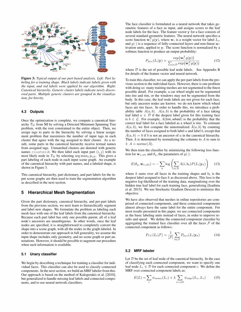
Figure 3: Typical output of our part based analysis. Left: Part la-beling for a training shape. Black labels indicate labels given withthe input, and red labels were applied by our algorithm. Right:Canonical hierarchy. Generic cluster labels indicate newly discov-ered parts. Multiple generic clusters are grouped in the visualiza-tion, for brevity.

4.3 Outputs

Once the optimization is complete, we compute a canonical hier-archy TM from M by solving a Directed Minimum Spanning Treeproblem, with the root constrained to the entire object. Then, weassign tags to parts in the hierarchy by solving a linear assign-ment problem that maximizes the number of input tags in eachcluster that agree with the tag assigned to their cluster. As a re-sult, some parts in the canonical hierarchy receive textual namesfrom assigned tags. Unmatched clusters are denoted with genericnames cluster N. We then label each input part (i, j) with itsmost likely node in TM by selecting arg maxk pijk. This gives apart labeling of each node in each input scene graph. An exampleof the canonical hierarchy with part names, and a labeled shape, isshown in Figure 3.

This canonical hierarchy, part dictionary, and part labels for the in-put scene graphs are then used to train the segmentation algorithmas described in the next section.

5 Hierarchical Mesh Segmentation

Given the part dictionary, canonical hierarchy, and per-part labelsfrom the previous section, we next learn to hierarchically segmentand label new shapes. We formulate the problem as labeling eachmesh face with one of the leaf labels from the canonical hierarchy.Because each part label has only one possible parent, all of a leafnode’s ancestors are unambiguous. In other words, once the leafnodes are specified, it is straightforward to completely convert theshape into a scene graph, with all the nodes in the graph labeled. Inorder to demonstrate our approach in full generality, we assume theinput shape includes only geometry, and no scene graph or part an-notations. However, it should be possible to augment our procedurewhen such information is available.

5.1 Unary classifier

We begin by describing a technique for training a classifier for indi-vidual faces. This classifier can also be used to classify connectedcomponents. In the next section, we build an MRF labeler from this.Our approach is based on the method of Kalogerakis et al. [2010],but generalized to handle missing leaf labels and connected compo-nents, and to use neural network classifiers.

The face classifier is formulated as a neural network that takes ge-ometric features of a face as input, and assigns scores to the leafnode labels for the face. The feature vector y for a face consists ofseveral standard geometric features. The neural network specifies ascore function wT

i g(y), where wi is a weight vector for label Li,and g(·) is a sequence of fully-connected layers and non-linear ac-tivation units, applied to y. The score function is normalized by asoftmax function to produce an output probability:

Pface(Li|y) =exp(wT

i g(y))∑

j∈D exp(wT

j g(y)) (12)

where D is the set of possible leaf node labels. See Appendix Bfor details of the feature vector and neural network.

To train this classifier, we can apply the per-part labels from the pre-vious section to the individual faces. However, there is one problemwith doing so: many training meshes are not segmented to the finestpossible detail. For example, a car wheel might not be segmentedinto tire and rim, or the windows may not be segmented from thebody. In this case, the leaf node labels are not given for each face,but only ancestor nodes are known: we do not know which wheelfaces are tire faces. In order to handle this, we introduce a prob-ability table A(a, b). A(a, b) is the probability of a face takingleaf label a ∈ D if the deepest label given for this training faceis b ∈ L. For example, A(tire,wheel) is the probability that thecorrect leaf label for a face labeled as a wheel is tire. To estimateA(a, b), we first compute the unnormalized A(a, b) by countingthe number of faces assigned to both label a and label b, except thatA(a, b) = 0 if b is not an ancestor of a in the canonical hierarchy.Then A is determined by normalizing the columns to A to sum to1: A = normc(A).

We then train the classifier by minimizing the following loss func-tion for w1:|D| and θg , the parameters of g(·):

E(θg,w1:|D|) = −∑k

log

(∑i∈D

A(i, bk)P (Li|yk)

)(13)

where k sums over all faces in the training shapes and bk is thedeepest label assigned to face k as discussed above. This loss is thenegative log-likelihood of the training data, marginalizing over thehidden true leaf label for each training face, generalizing [Izadiniaet al. 2015]. We use Stochastic Gradient Descent to minimize thisobjective.

We have also observed that meshes in online repositories are com-prised of connected components, and these connected componentsalmost always have the same label for the entire component. Formost results presented in this paper, we use connected componentsas the basic labeling units instead of faces, in order to improve re-sults and speed. We define the connected component classifier byaggregating the trained face classifier over all the faces F of theconnected component as follows:

PCC (Li|F) =1

|F|∑k∈F

Pface(Li|yk) (14)

5.2 MRF labeler

Let D be the set of leaf node of the canonical hierarchy. In the caseof classifying each connected component, we want to specify oneleaf node Lc ∈ D for each connected component c. We define theMRF over connected component labels as:

E(L) =∑c

ψunary(Lc) + λ∑

u,v∈E

ψedge(Lu, Lv) (15)

100 101 102 103 104

# Scene Graph Nodes

0

500

1000

1500

2000

2500

3000#

Shap

escarairplanechairrifle

Figure 4: Histogram of number of scene nodes for each shape inthe raw datasets.

with weight λ is set by cross-validation separately for each shapecategory and held constant across all experiments. The unary termψunary assesses the likelihood of component c having a given leaflabel, based on geometric features of the component, and is givenby the classifier:

ψunary(L) = − lnPCC (L|F) (16)

The edge term prefers adjacent components to have the same la-bel. It is defined as ψedge(Lu, Lv) = td(u, v), where td(Lu, Lv)is tree distance between labels Lu and Lv in the canonical hi-erarchy. This encourages adjacent labels to be as close in thecanonical hierarchy as possible. For example, ψ is 0 when thetwo labels are the same, whereas ψ is 2 if they are different butshare a common parent. To generate the edge set E in 15, weconnect K nearest connected components with this edge, whereK = min(30, d0.01Ncce) where Ncc is the number of connectedcomponents in the mesh.

Once the classifiers and λ are trained, the model can be applied toa new mesh as follows. First, the leaf labels are determined by op-timizing Equation 15 using the α-β swap algorithm [Boykov et al.2001]. Then, the scene graph is computed by bottom-up group-ing. In particular, adjacent components with same leaf label arefirst grouped together. Then, adjacent groups with the same parentare grouped at the next level of the hierarchy, and so on.

For the case where connected components are not available, theMRF algorithm is applied for each face. The unary term is givenby the face classifier ψunary(L) = − lnPface(L|F). We still needto handle the case where the object is not topologically connected,and so the pairwise term ψedge(Lu, Lv) applies to all faces u and vwhose centroids fall into theK-nearest neighborhood of each other,and is given by:

ψedge(Lu, Lv) = λt exp

(−κ1

2φu,v

π−

d2u,v

2(κ2dr)2

)td(Lu, Lv)

(17)where φu,v is the angle between the faces, du,v is the distance be-tween the face centroids, dr is the average distance between a face’scentroid and it’s nearest face’s centroid, and κ1 = 5, κ2 = 2.5 inall our experiments. λt is a scale factor to promote faces sharing an

edge: λt =

{10 if faces (u, v) share an edge,1 otherwise.

6 Results

In this section we evaluate our method on “in the wild” data frompublic online repositories and on a standard benchmark. We per-

form the evaluation by comparing with part-based analysis and seg-mentation techniques using novel metrics.

Input Data. We run our method on 9 shape categories fromShapeNetCore dataset [Chang et al. 2015], a collection of 3D mod-els obtained from various online repositories. We use this datasetfor convenience, because the data has been preprocessed, cleaned,categorized, and put into common formats; at present, it is the onlyknown current dataset that satisfies our low-level preprocessing re-quirements. We excluded most categories (∼40) because they onlyhave a few hundred shapes or less, which is inadequate for our ap-proach. We assume that a tag is sufficiently represented if it appearsin at least 25 shapes, and we only analyze categories that have morethan 2 such tags. Some categories have trivial geometry (e.g., mo-bile phones). Some categories do not provide enough parts withcommon labels (e.g., watercraft are very heterogeneous to the pointof being disjoint sets of objects). The ShapeNetCore dataset cur-rently contains a small subset of the available online repositories,which limits the data that we have immediately at hand. However,ShapeNetCore is growing; applying our method to much largerdatasets is limited only by the nuisance of preprocessing hetero-geneous datasets.

Typical scene graphs in such online repositories are very diverse,including between one and thousands of nodes (Figure 4), and rang-ing from flat to deep hierarchies (Figure 5). For each category, wealso prescribe a list of relevant tags and possible synonyms. Weautomatically create a list of most-used tags for the entire category,and then manually pick relevant English nouns as the tag dictionary.Note that only a fraction of shapes have any parts with the chosentags, and the frequency distribution over tag names is very uneven(Table 1, Init column).

For a categories with ∼2000 shapes, the part-based analysis takesapproximately one hour, and the segmentation training takes ap-proximately 10 hours, each on a single Titan X GPU. Once trained,analysis of a new shape typically takes about 25 seconds, of whichabout 15 seconds is extracting face features with non-optimizedMatlab code.

Hierarchical Mesh Segmentation and Labeling. Figure 10demonstrates some representative results produced by our hierar-chical segmentation based on connected components (Section 5).The resulting hierarchical segmentation vary in depth from flat(e.g., chairs) to deep (e.g., cars, airplanes), reflecting complexityof the corresponding object. We also often extract consistent partclusters, even if they do not have textual tags. We found that ana-lyzing shapes at the granularity of connected components is usuallysufficient: the mean number of connected components per object inShapeNet is 4169, and the largest connected component in shapescovers only 9.58% of the total surface area on average: connectedcomponents tend to be small. These components are often alignedto part boundaries, for example, if one was to annotate ShapeNetSegmentation benchmark [Yi et al. 2016] by assigning a majoritylabel to each connected component they would get 94% of facescorrect.

Segmentation without Connected Components. In the caseof applying per-face labeling, when connected components are notavailable, we observe similar results with this method as to thosewhere the connected components are used. However, a few seg-ments do not come out as cleanly-segmented on more complexmodels (see Figure 11). Please refer to our supplementary mate-rial for qualitative results of this experiment. We tested our methodon other datasets (Thingi10k [Zhou and Jacobson 2016], COSEG[Wang et al. 2012]), but were only able to test on a limited set of

# Levels1 2 3 4 5 6 7 8 9 10

Per

cent

age

of S

hape

s

0

0.05

0.1

0.15

0.2

0.25

0.3

0.35

0.4

0.45carairplanechairrifle

Figure 5: Histogram of number of levels in hierarchy for eachshape in the raw datasets.

models, since only a few models in these datasets come from ourtraining categories.

Tag prediction. Table 1, Final column shows what fraction oftraining shapes received a particular tag after our part-based analy-sis (Section 4). Note that an object may be missing a tag for severalpossible reasons: it could be misclassified, or because the objectdoes not have that part, or does not have it segmented as a separatescene graph node. As evident from this quantitative analysis, theamount of training data we can use in subsequent analysis has dras-tically increased. Please refer to supplementary material for visualexamples from labeling results.

To evaluate tag prediction accuracy, we perform the following ex-periment. We hold out 30% of the tagged parts during training, andevaluate labeling accuracy on these parts. As our method is basedon nearest-neighbors (NN) classification, we compare against NNon features computed in the following ways: (1) clustering withLFD, (2) clustering with x, (3) our method with no Ec term, and(4) No Em term. Results are reported in Table 3. As shown in thetable, our method significantly improves tag classification perfor-mance over the baselines. This experiment also demonstrates thevalue of our clustering and hierarchy terms Ec and Em.

Cluster evaluation. Figure 6 (bottom) demonstrates some partsgrouped by our method in the part-based analysis (Section 4). Wealso note that some clusters combine unrelated parts, and we believethat they serve as null clusters for outliers.

As we do not have ground truth for the unlabeled clusters, we in-stead evaluate the ability of our learned embedding to cluster parts,with the user-provided labels can serve as ground truth. We split thedataset for a category into training tags and test tags. We run thepart-based analysis on all shapes, but provide only the training sub-set of tags to the algorithm. This gives an embedding f , and we canevaluate how good f is for clustering. This is done by running k-means clustering on the parts that correspond to the test tags, with kset to the number of test tags. The clustering result is then comparedto the test tag labeling by normalized Mutual Information. This pro-cess is repeated in a 3-fold cross-validation. The baseline scores areespecially low on categories with few parts, like Bus and Table. Ta-ble 2 shows quantitative results; our method performs significantlybetter than the baselines, including using k-means on Light FieldDescriptors (LFD), and omitting the clustering term Ec from theobjective.

Comparison to Unsupervised Co-Hierarchy. Van Kaick et al.[2013] propose an unsupervised approach for establishing consis-

Table 1: Tags and their frequency (percent of shapes that have ascene node (i.e., part) labeled with the corresponding tag) in theraw datasets and after our part based processing.

Part Init Final Part Init Final Part Init FinalCategory: Car (2287 shapes)

Wheel 17.4 96.4 Mirror 6.9 68.2 Window 9.5 71.8Fender 1.1 40.4 Bumper 15.2 63.0 Roof 2.4 48.2Exhaust 7.2 57.5 Floor 2.6 49.9 Trunk 4.5 60.6

Door 19.9 67.8 Spoiler 2.8 41.3 Rim 4.1 74.1Headlight 14.6 61.9 Hood 12.2 68.7 Tire 5.3 33.5

Category: Airplane (2574 shapes)Wing 5.9 86.9 Engine 5.5 81.6 Body 2.3 86.8Tail 1.5 90.5 Missile 0.4 66.7

Category: Chair (2401 shapes)Arm 1.5 62.4 Leg 3.6 71.0 Back 0.9 50.8Seat 2.4 83.1 Wheel 1.4 34.6

Category: Table (2355 shapes)Top 1.9 81.5 Leg 6.4 85.8

Category: Sofa (1243 shapes)BackPillow 4.7 79.3 Seat 2.7 63.0 Feet 3.1 41.5

Category: Rifle (994 shapes)Barrel 1.2 62.9 Bipod 1.7 47.6 Scope 3.2 66.7Stock 3.2 56.0

Category: Bus (713 shapes)Seat 4.8 47.0 Wheel 8.3 88.9 Mirror 1.7 42.4

Category: Guitar (491 shapes)Neck 3.1 75.8 Body 0.8 67.6

Category: Motorbike (281 shapes)Seat 23.5 49.2 Engine 21.7 84.0 Gastank 14.6 73.7

Exhaust 1.8 71.5 Handle 8.9 75.8 Wheel 41.6 98.9

Figure 6: Visualization of typical clusters. Note that some clustershave labels that were propagated from the tags, whereas some havegeneric labels indicating that they were discovered without any taginformation.

tent hierarchies within an object category. Their method was devel-oped for small shape collections and requires hours of computationfor 20 models, which makes it unsuitable for ShapeNet data. Onthe other hand, since we assume that some segments have textualtags, we also cannot run our method on their data. Given theseconstraints, we show a qualitative comparison to their method. Inparticular, we picked the first car and first airplane in their dataset,and retrieved the most similar models in ShapeNet using lightfielddescriptors. Figure 7 demonstrates their and our hierarchies side-by-side. Note that our method generates more detailed hierarchiesand also provides textual tags for parts.

Figure 7: Comparison with [van Kaick et al. 2013]. We show ahierarchy produced by their approach (left) and a hierarchy of themost similar model in our database (right). Our hierarchies havelabels and provide finer details.

Comparison to Supervised Segmentation. Since there areno large-scale hierarchical segmentation benchmarks, we test ourmethod on the segmentation dataset provided by Yi et al. [2016].We emphasize that the benchmark contains much coarser segmen-tations than those we can produce, and does not include hierarchies.We take the intersection of our 9 categories and the benchmark,which yields the following six categories for quantitative evalua-tion: car, airplane, motorbike, guitar, chair, table.

Since other techniques do not leverage connected components, weevaluate per-face classification from unary terms only, comparingthe per-face classification prediction (Eq. 14) to results from Yi etal. [2016] trained only on benchmark data.

Our training data is sampled from a different data distribution thanthe benchmark; repurposing a model from one training set to an-other is a problem known as domain adaptation. The first approachwe test is to directly map the labels predicted by our classifier tobenchmark labels. The second approach is to obtain 5 training ex-amples from the benchmark, and train a Support Vector Machineclassifier to predict benchmark labels from our learned features{g(x)} (Sec. 4). The resulting classifier is the softmax of {ηig(x)},where ηi are the SVM parameters for ith label. As baseline fea-tures, we also test k-means clustering with LFD features over allinput parts, where k is the same as the number of clusters used byour method.

Results of supervised segmentation comparison experiments areshown in Figure 8. Without training on our features, the methodof Yi et al. [2016] requires 50-100 benchmark training examplesin order to match the results we get with only 5 benchmark exam-ples. Although our method is trained on many ShapeNet meshes,these meshes did not require any manual labeling. This illustrateshow our method, trained on freely-available data, can be cheaplyadapted to a new task.

Figure 9 shows qualitative results from comparison with Yi etal. [2016], where we use 10 models for training in [Yi et al. 2016]followed by the domain adaptation through using the same 10 mod-els in our approach.

0 20 40 60 80 100Number of Labeled Training Model

0.4

0.45

0.5

0.55

0.6

0.65

0.7

0.75

0.8

0.85

0.9

Aver

age

Per P

art I

nter

sect

ion

Ove

r Uni

on

Airplane

Yi et al. 2016LFD without CalibrationOurs without CalibrationLFD with CalibrationOurs with Calibration

0 20 40 60 80 100Number of Labeled Training Model

0.4

0.45

0.5

0.55

0.6

0.65

0.7

0.75

0.8

0.85

0.9

Aver

age

Per P

art I

nter

sect

ion

Ove

r Uni

on

CarYi et al. 2016LFD without CalibrationOurs without CalibrationLFD with CalibrationOurs with Calibration

0 20 40 60 80 100Number of Labeled Training Model

0.4

0.45

0.5

0.55

0.6

0.65

0.7

0.75

0.8

0.85

0.9

Aver

age

Per P

art I

nter

sect

ion

Ove

r Uni

on

Chair

Yi et al. 2016LFD without CalibrationOurs without CalibrationLFD with CalibrationOurs with Calibration

0 20 40 60 80 100Number of Labeled Training Model

0.4

0.45

0.5

0.55

0.6

0.65

0.7

0.75

0.8

0.85

0.9

Aver

age

Per P

art I

nter

sect

ion

Ove

r Uni

on

Guitar

Yi et al. 2016LFD without CalibrationOurs without CalibrationLFD with CalibrationOurs with Calibration

0 20 40 60 80 100Number of Labeled Training Model

0.4

0.45

0.5

0.55

0.6

0.65

0.7

0.75

0.8

0.85

0.9

Aver

age

Per P

art I

nter

sect

ion

Ove

r Uni

on

MotorbikeYi et al. 2016LFD without CalibrationOurs without CalibrationLFD with CalibrationOurs with Calibration

0 20 40 60 80 100Number of Labeled Training Model

0.4

0.45

0.5

0.55

0.6

0.65

0.7

0.75

0.8

0.85

0.9

Aver

age

Per P

art I

nter

sect

ion

Ove

r Uni

on

Table

Yi et al. 2016LFD without CalibrationOurs without CalibrationLFD with CalibrationOurs with Calibration

Figure 8: Comparison with [Yi et al. 2016]. Segmentation accu-racy scores are shown; higher is better. The blue curves show theresults of Yi et al. as a function of training set size. The red dashedlines show the result of our method without applying domain adap-tion, and the red solid lines show our method with domain adap-tation by training on 5 benchmark models. For the more complexclasses, Yi et al.’s method requires 50-100 training meshes to matchour performance with only 5 benchmark training meshes.

Figure 9: Qualitative comparison with [Yi et al. 2016]. For a faircomparison, we use 10 models for training in [Yi et al. 2016] andwe use the same 10 models for domain adaptation in our approach.

7 Discussions and Conclusion

We have proposed a novel method for mining consistent hierarchi-cal shape models from massive but sparsely annotated scene graphs“in the wild.” As we analyze the input data, we jointly embed partsto a low-dimensional feature space, cluster corresponding parts, andbuild a probabilistic model for hierarchical relationships amongthem. We demonstrated that our model can facilitate hierarchicalmesh segmentation and were able to extract complex hierarchiesand identify small segments in 3D models from various shape cat-

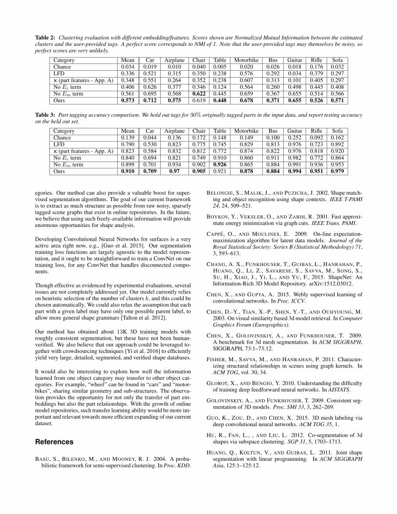
Table 2: Clustering evaluation with different embedding/features. Scores shown are Normalized Mutual Information between the estimatedclusters and the user-provided tags. A perfect score corresponds to NMI of 1. Note that the user-provided tags may themselves be noisy, soperfect scores are very unlikely.

Category Mean Car Airplane Chair Table Motorbike Bus Guitar Rifle SofaChance 0.034 0.019 0.010 0.040 0.005 0.020 0.026 0.018 0.176 0.032LFD 0.336 0.521 0.315 0.350 0.238 0.576 0.292 0.034 0.379 0.297x (part features - App. A) 0.348 0.551 0.264 0.352 0.238 0.607 0.313 0.101 0.405 0.297No Ec term 0.406 0.626 0.377 0.346 0.124 0.564 0.260 0.498 0.445 0.408No Em term 0.561 0.695 0.568 0.622 0.445 0.659 0.367 0.655 0.514 0.566Ours 0.573 0.712 0.575 0.619 0.448 0.678 0.371 0.655 0.526 0.571

Table 3: Part tagging accuracy comparison. We hold out tags for 30% originally tagged parts in the input data, and report testing accuracyon the held out set.

Category Mean Car Airplane Chair Table Motorbike Bus Guitar Rifle SofaChance 0.139 0.044 0.136 0.172 0.148 0.149 0.100 0.252 0.092 0.162LFD 0.790 0.530 0.823 0.775 0.745 0.829 0.813 0.976 0.723 0.892x (part features - App. A) 0.823 0.584 0.832 0.812 0.772 0.874 0.822 0.976 0.818 0.920No Ec term 0.840 0.694 0.821 0.749 0.910 0.860 0.911 0.982 0.772 0.864No Em term 0.899 0.701 0.934 0.902 0.926 0.865 0.884 0.991 0.936 0.953Ours 0.910 0.709 0.97 0.905 0.921 0.878 0.884 0.994 0.951 0.979

egories. Our method can also provide a valuable boost for super-vised segmentation algorithms. The goal of our current frameworkis to extract as much structure as possible from raw noisy, sparselytagged scene graphs that exist in online repositories. In the future,we believe that using such freely-available information will provideenormous opportunities for shape analysis.

Developing Convolutional Neural Networks for surfaces is a veryactive area right now, e.g., [Guo et al. 2015]. Our segmentationtraining loss functions are largely agnostic to the model represen-tation, and it ought to be straightforward to train a ConvNet on ourtraining loss, for any ConvNet that handles disconnected compo-nents.

Though effective as evidenced by experimental evaluations, severalissues are not completely addressed yet. Our model currently relieson heuristic selection of the number of clusters k, and this could bechosen automatically. We could also relax the assumption that eachpart with a given label may have only one possible parent label, toallow more general shape grammars [Talton et al. 2012].

Our method has obtained about 13K 3D training models withroughly consistent segmentation, but these have not been human-verified. We also believe that our approach could be leveraged to-gether with crowdsourcing techniques [Yi et al. 2016] to efficientlyyield very large, detailed, segmented, and verified shape databases.

It would also be interesting to explore how well the informationlearned from one object category may transfer to other object cat-egories. For example, “wheel” can be found in “cars” and “motor-bikes”, sharing similar geometry and sub-structures. The observa-tion provides the opportunity for not only the transfer of part em-beddings but also the part relationships. With the growth of onlinemodel repositories, such transfer learning ability would be more im-portant and relevant towards more efficient expanding of our currentdataset.

References

BASU, S., BILENKO, M., AND MOONEY, R. J. 2004. A proba-bilistic framework for semi-supervised clustering. In Proc. KDD.

BELONGIE, S., MALIK, J., AND PUZICHA, J. 2002. Shape match-ing and object recognition using shape contexts. IEEE T-PAMI24, 24, 509–521.

BOYKOV, Y., VEKSLER, O., AND ZABIH, R. 2001. Fast approxi-mate energy minimization via graph cuts. IEEE Trans. PAMI.

CAPPE, O., AND MOULINES, E. 2009. On-line expectation-maximization algorithm for latent data models. Journal of theRoyal Statistical Society: Series B (Statistical Methodology) 71,3, 593–613.

CHANG, A. X., FUNKHOUSER, T., GUIBAS, L., HANRAHAN, P.,HUANG, Q., LI, Z., SAVARESE, S., SAVVA, M., SONG, S.,SU, H., XIAO, J., YI, L., AND YU, F., 2015. ShapeNet: AnInformation-Rich 3D Model Repository. arXiv:1512.03012.

CHEN, X., AND GUPTA, A. 2015. Webly supervised learning ofconvolutional networks. In Proc. ICCV.

CHEN, D.-Y., TIAN, X.-P., SHEN, Y.-T., AND OUHYOUNG, M.2003. On visual similarity based 3d model retrieval. In ComputerGraphics Forum (Eurographics).

CHEN, X., GOLOVINSKIY, A., AND FUNKHOUSER, T. 2009.A benchmark for 3d mesh segmentation. In ACM SIGGRAPH,SIGGRAPH, 73:1–73:12.

FISHER, M., SAVVA, M., AND HANRAHAN, P. 2011. Character-izing structural relationships in scenes using graph kernels. InACM TOG, vol. 30, 34.

GLOROT, X., AND BENGIO, Y. 2010. Understanding the difficultyof training deep feedforward neural networks. In AISTATS.

GOLOVINSKIY, A., AND FUNKHOUSER, T. 2009. Consistent seg-mentation of 3D models. Proc. SMI 33, 3, 262–269.

GUO, K., ZOU, D., AND CHEN, X. 2015. 3D mesh labeling viadeep convolutional neural networks. ACM TOG 35, 1.

HU, R., FAN, L., , AND LIU, L. 2012. Co-segmentation of 3dshapes via subspace clustering. SGP 31, 5, 1703–1713.

HUANG, Q., KOLTUN, V., AND GUIBAS, L. 2011. Joint shapesegmentation with linear programming. In ACM SIGGRAPHAsia, 125:1–125:12.

Figure 10: Hierarchical segmentation results. In each case, the input is a geometric shape. Our method automatically determines thesegmentation into parts, the part labels and the hierarchy.

Figure 11: Hierarchical segmentation results with and without theconnected components assumption. Even without connected com-ponents, our method estimates complex hierarchical structures. Forsome models, the boundaries are less precise (see red higlights). Weprovide a full comparison to Figure 10 in supplemental material.

HUANG, Q., WANG, F., AND GUIBAS, L. 2014. Functional mapnetworks for analyzing and exploring large shape collections.SIGGRAPH 33, 4.

IZADINIA, H., RUSSELL, B. C., FARHADI, A., HOFFMAN,M. D., AND HERTZMANN, A. 2015. Deep classifiers fromimage tags in the wild. In Proc. Multimedia COMMONS.

JELINEK, F., LAFFERTY, J. D., AND MERCER, R. L. 1992. Ba-sic methods of probabilistic context free grammars. In SpeechRecognition and Understanding. Springer, 345–360.

JOHNSON, A. E., AND HEBERT, M. 1999. Using spin images forefficient object recognition in cluttered 3d scenes. IEEE T-PAMI21, 5, 433–449.

KALOGERAKIS, E., HERTZMANN, A., AND SINGH, K. 2010.Learning 3d mesh segmentation and labeling. ACM Transactionson Graphics (TOG) 29, 4, 102.

KIM, V. G., LI, W., MITRA, N. J., CHAUDHURI, S., DIVERDI,S., AND FUNKHOUSER, T. 2013. Learning part-based tem-plates from large collections of 3d shapes. ACM Transactions onGraphics (TOG) 32, 4, 70.

KINGMA, D. P., AND BA, J. L. 2015. Adam: A method forstochastic optimization. In Proc. ICLR.

LI, X., URICCHIO, T., BALLAN, L., BERTINI, M., SNOEK, C.G. M., AND BIMBO, A. D. 2016. Socializing the semantic gap:A comparative survey on image tag assignment, refinement, andretrieval. ACM Comput. Surv. 49, 1.

LIU, T., CHAUDHURI, S., KIM, V. G., HUANG, Q.-X., MITRA,N. J., AND FUNKHOUSER, T. 2014. Creating Consistent SceneGraphs Using a Probabilistic Grammar. SIGGRAPH Asia 33, 6.

MITRA, N. J., WAND, M., ZHANG, H., COHEN-OR, D., ANDBOKELOH, M. 2013. Structure-aware shape processing. InEurographics STARs, 175–197.

NEAL, R. M., AND HINTON, G. E. 1998. A view of the emalgorithm that justifies incremental, sparse, and other variants.In Learning in graphical models. Springer, 355–368.

ORDONEZ, V., KULKARNI, G., AND BERG, T. L. 2011. Im2text:Describing images using 1 million captioned photographs. InProc. NIPS.

OSADA, R., FUNKHOUSER, T., CHAZELLE, B., AND DOBKIN,D. 2002. Shape distributions. ACM Transactions on Graphics.

PORTER, M. F. 1980. An algorithm for suffix stripping. Program14, 3, 130–137.

SIDI, O., VAN KAICK, O., KLEIMAN, Y., ZHANG, H., ANDCOHEN-OR, D. 2011. Unsupervised co-segmentation of a setof shapes via descriptor-space spectral clustering. ACM SIG-GRAPH Asia 30, 6, 126:1–126:9.

TALTON, J., YANG, L., KUMAR, R., LIM, M., GOODMAN, N.,AND MECH, R. 2012. Learning design patterns with bayesiangrammar induction. In UIST.

TIGHE, J., AND LAZEBNIK, S. 2011. Understanding scenes onmany levels. In Proc. ICCV.

TORRESANI, L. 2016. Weakly-supervised learning. In ComputerVision: A Reference Guide, K. Ikeuchi, Ed.

VAN KAICK, O., XU, K., ZHANG, H., WANG, Y., SUN, S.,SHAMIR, A., AND COHEN-OR, D. 2013. Co-hierarchical anal-ysis of shape structures. ACM Transactions on Graphics (TOG)32, 4, 69.

WANG, Y., XU, K., LI, J., ZHANG, H., SHAMIR, A., LIU, L.,CHENG, Z., AND XIONG, Y. 2011. Symmetry Hierarchy ofMan-Made Objects. Eurographics 30, 2.

WANG, Y., ASAFI, S., VAN KAICK, O., ZHANG, H., COHEN-OR, D., AND CHENAND, B. 2012. Active co-analysis of a setof shapes. SIGGRAPH Asia.

XIE, Z., XU, K., LIU, L., AND XIONG, Y. 2014. 3d shape seg-mentation and labeling via extreme learning machine. SGP.

XU, K., KIM, V. G., HUANG, Q., MITRA, N. J., AND KALOGER-AKIS, E. 2016. Data-driven shape analysis and processing. SIG-GRAPH Asia Course.

YI, L., KIM, V. G., CEYLAN, D., SHEN, I., YAN, M., SU, H.,LU, C., HUANG, Q., SHEFFER, A., AND GUIBAS, L. 2016.A scalable active framework for region annotation in 3d shapecollections. TOG 35, 6, 210.

YUMER, M. E., CHUN, W., AND MAKADIA, A. 2014. Co-segmentation of textured 3d shapes with sparse annotations. In2014 IEEE Conference on Computer Vision and Pattern Recog-nition, IEEE, 240–247.

ZHOU, Q., AND JACOBSON, A., 2016. Thingi10k: A dataset of10,000 3d-printing models. arxiv:1605.04797.

A Part Features and Embedding Network

We compute per-part geometric features which are further used forjoint part embedding and clustering (Section 4). The feature vectorxij includes 3-view lightfield descriptor [Chen et al. 2003] (withHOG features for each view), center-of-mass, bounding box di-ameter, approximate surface area (fraction of voxels occupied in30x30x30 object grid), and local frame in PCA coordinate system(represented by 3 × 3 matrix M ). To mitigate reflection ambigui-ties for local frame we constraint all frame axes to have positive dot

Figure 12: Embedding network f architecture for parts. Differentinput part features go through a stack of fully connected layers andthen are concatenated and go through additional fully connect lay-ers to generate output of f . The contrastive loss also takes output ofanother part, from an identical embedding branch as input, whichis omitted in this figure for brevity.

Table 4: Embedding network f output dimensionalities after eachlayer.

feature fc1 fc2 fc3 concat fc4 fc5 fc6LFD 128 256 256

512 256 128 64PCA Frame 16 32 64CoM 16 64 64Diameter 8 32 64Area 8 32 64

product with z-axis (typically up) of the global frame. For lightfielddescriptor we normalize the part to be centered at origin and havebounding box diameter 1, for all other descriptors we normalize themesh in the same way. We mitigate reflection ambiguities by con-straining all frame axes to have positive dot product with the z-axisof the global frame. The neural network embedding f is visualizedin Figure 12, and, in Table 4, we show the embedding network pa-rameters, where we alter first few fully connected layers to allocatemore neurons for richer features such as LFD.

B Face Features and Classifier Network

We compute per-face geometric features y which are furtherused for hierarchical mesh segmentation (Section 5). Thesefeatures include spin images (SI) [Johnson and Hebert 1999],shape context (SC) [Belongie et al. 2002], distance distribu-tion (DD) [Osada et al. 2002], local PCA (LPCA) (where λi

are eigenvalues of local coordinate system, and features areλ1/

∑λi, λ2/

∑λi, λ3/

∑λi, λ2/λ1, λ3/λ1, λ3/λ2), local point

position variance (LVar), curvature, point position (PP) and normal(PN). To compute local radius for the feature computation we sam-ple 10000 points on the entire shape and use 50 nearest neighbors.We use the same architecture as part embedding network f (Fig. 12)for face classification, but with different loss function (Eq. 13) andnetwork parameters, which are summarized in Table 5.

Table 5: Face classification network parameters.feature fc1 fc2 fc3 concat fc4 fc5 fc6Curvature 32 64 64

640 256 128 128

LPCA 64 64 64LVar 32 64 64SI 128 128 128SC 128 128 128DD 32 64 64PP 16 32 64PN 16 32 64

C E-step Update

In the E-step, the assignment probabilities are iteratively updated.For each node (i, j), the probability that it is assigned to label k isupdated as:

p∗ijk ← exp

λm

∑a∈C(i,j),`

pia` lnMk` + λm

∑b=P (i,j),`

pib` lnM`k

−λc||f(xij − ck||1) (18)

pijk ←p∗ijk∑` p∗ij`

(19)

where C(i, j) is set of children of node (i, j) and P (i, j) is theparent node. A joint closed-form update to all assignments couldbe computed using Belief Propagation, but we did not try this.