learning from the flood of findings: meta-analysis in … from the flood of findings: meta-analysis...
TRANSCRIPT

Learning from the Flood of Findings:
Meta-Analysis in Economics
Jacques Poot National Institute of Demographic and Economic Analysis (NIDEA)
University of Waikato
with thanks to: Raymond Florax, Purdue University Luana Dow, University of Waikato

Outline • What is meta-analysis?
• Why do it?
• History
• Current practice in economics
• The recipe
• Example 1: does migration affect trade?
• The statistical theory
• Example 2: the "wage curve" and publication bias
• Example 3: the lifecycle hypothesis and global savings
• The future
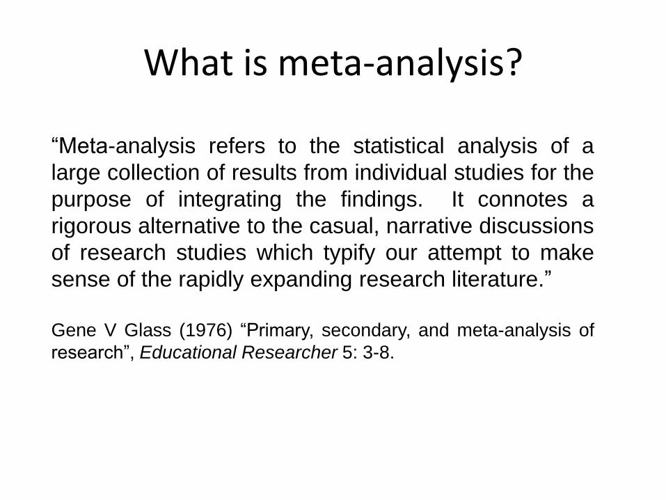
What is meta-analysis?
“Meta-analysis refers to the statistical analysis of a
large collection of results from individual studies for the
purpose of integrating the findings. It connotes a
rigorous alternative to the casual, narrative discussions
of research studies which typify our attempt to make
sense of the rapidly expanding research literature.”
Gene V Glass (1976) “Primary, secondary, and meta-analysis of
research”, Educational Researcher 5: 3-8.
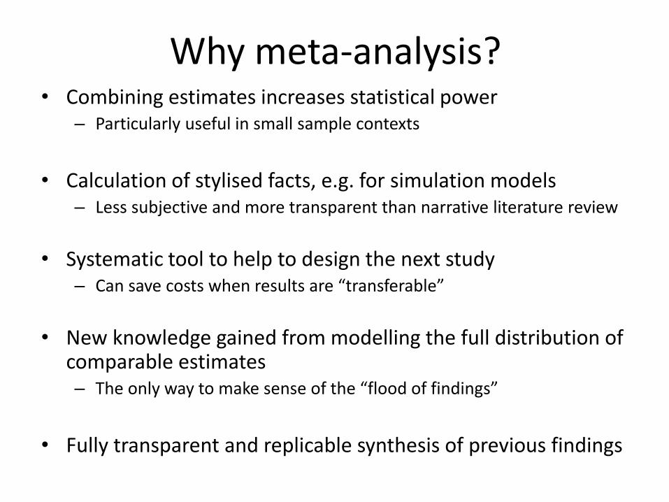
Why meta-analysis? • Combining estimates increases statistical power
– Particularly useful in small sample contexts
• Calculation of stylised facts, e.g. for simulation models – Less subjective and more transparent than narrative literature review
• Systematic tool to help to design the next study – Can save costs when results are “transferable”
• New knowledge gained from modelling the full distribution of comparable estimates – The only way to make sense of the “flood of findings”
• Fully transparent and replicable synthesis of previous findings
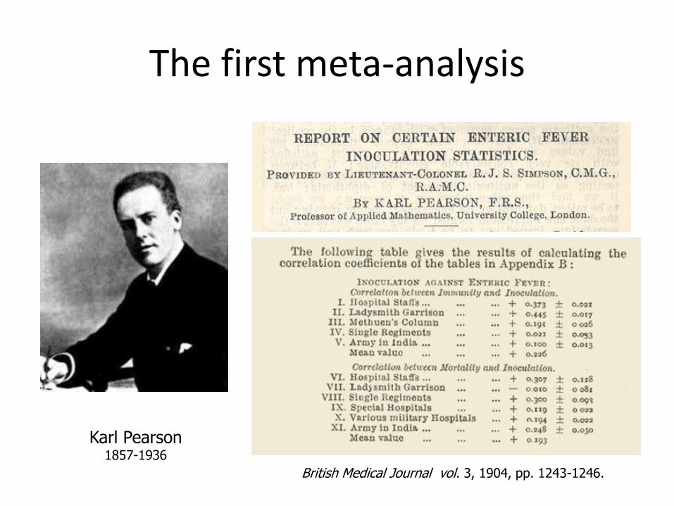
The first meta-analysis
Karl Pearson 1857-1936
British Medical Journal vol. 3, 1904, pp. 1243-1246.

Modern meta-analysis
Gene Glass
Example: Glass, G.V. and Smith M.L. (1979) Meta-analysis of research on class
size and achievement Educational Evaluation and Policy Analysis 1(1): 2-16
Effect size: ∆𝑆−𝐿=𝑋 𝑆−𝑋 𝐿
𝜎
Data: 77 studies (1902-1972; 900,000 pupils) from about a dozen countries yielded 725 ∆𝑆−𝐿
Conclusion: “There is little doubt that, other things equal, more is learned in smaller classes”

Meta-analysis in economics
Tom Stanley
Stanley, T.D. and Jarrell, S.B. (1989) Meta-regression
analysis: a quantitative method of literature surveys.
Journal of Economic Surveys 3: 54-67.
Stanley, T.D. (2001) Wheat from Chaff: Meta-analysis as
quantitative literature review. Journal of Economic
Perspectives 15(3): 131-150.
Journal of Economics Surveys – online conference
November 16-18 2011 Communications with Economists:
Current and Future Trends
http://joesonlineconference.wordpress.com/
Also: special JES issues in 2005 and 2011

The meta-analysis “industry”
• Systematic review
– Cochrane collaboration (medical research; www.cochrane.org.nz)
– Campbell collaboration (education, crime and justice, social welfare; www.campbellcollaboration.org)
– International Initiative for Impact Evaluation - 3ie (development; www.3ieimpact.org)
• Meta-analysis in economics
– MAER-net, http://www.hendrix.edu/maer-network/

Meta-Meta-Analysis in Economics, n = 626
Starting with: Nelson JP (1980) Airports and property values: A survey of
recent evidence. Journal of Transport Economics and Policy 14(1): 37-52.
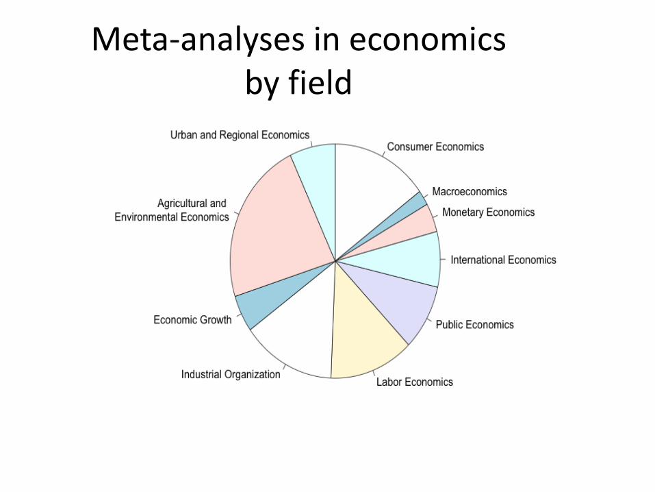
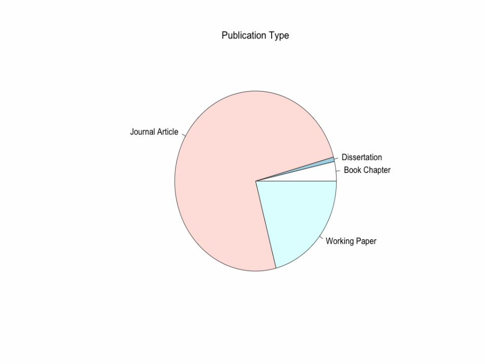
Meta-analyses in economics by field
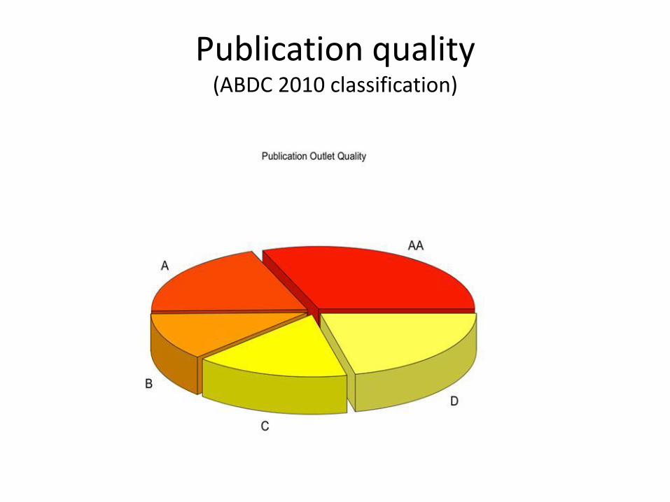
Publication quality (ABDC 2010 classification)

Top 6 Meta-Analyses in “Core” Economics Criterion: Google Scholar cites per year
Kluve J (2010)
The effectiveness of European active labor
market programs Labour Economics 141
Viscusi WK and Aldy JE
(2003)
The value of a statistical life: A critical review of
market estimates throughout the world
Journal of Risk and
Uncertainty 85
Disdier AC and Head K
(2008)
The puzzling persistence of the distance effect
on bilateral trade
Review of Economics
and Statistics 82
Djankov S and Murell P
(2002)
Enterprise restructuring in transition: A
quantitative survey
Journal of Economic
Literature 81
Card D, Kluve J and
Weber A (2010)
Active labour market policy evaluations: A meta-
analysis The Economic Journal 67
Görg H and Strobl
(2001)
Multinational companies and productivity
spillovers: A meta-analysis The Economic Journal 50
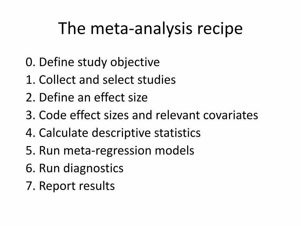
The meta-analysis recipe
0. Define study objective
1. Collect and select studies
2. Define an effect size
3. Code effect sizes and relevant covariates
4. Calculate descriptive statistics
5. Run meta-regression models
6. Run diagnostics
7. Report results

Example 1: Does migration affect trade? -.
20
.2.4
.6
Qu
an
tile
s o
f m
igra
tio
n e
lasticity o
f exp
ort
s
0 .25 .5 .75 1Fraction of the data
-.2
0.2
.4.6
Qu
an
tile
s o
f m
igra
tio
n e
lasticity o
f im
port
s
0 .25 .5 .75 1Fraction of the data
Exports Imports
48 studies (233 export and 178 import effect sizes), starting with DM Gould (1994) “Immigrant links to the home country: empirical implications for US bilateral trade flows” REStat Source: Nijkamp, Poot and Sahin (eds) (2012) Migration Impact Assessment, Edward Elgar.
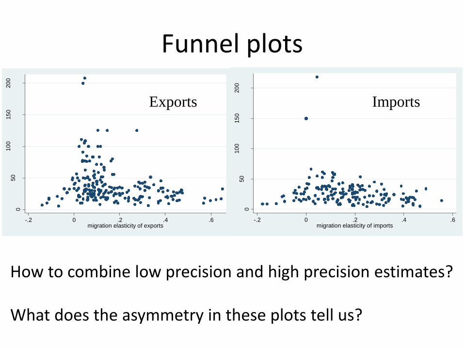
Funnel plots 0
50
10
015
020
0
xbp
recis
ion
-.2 0 .2 .4 .6migration elasticity of exports
050
10
015
020
0
mbp
recis
ion
-.2 0 .2 .4 .6migration elasticity of imports
How to combine low precision and high precision estimates? What does the asymmetry in these plots tell us?
Exports Imports
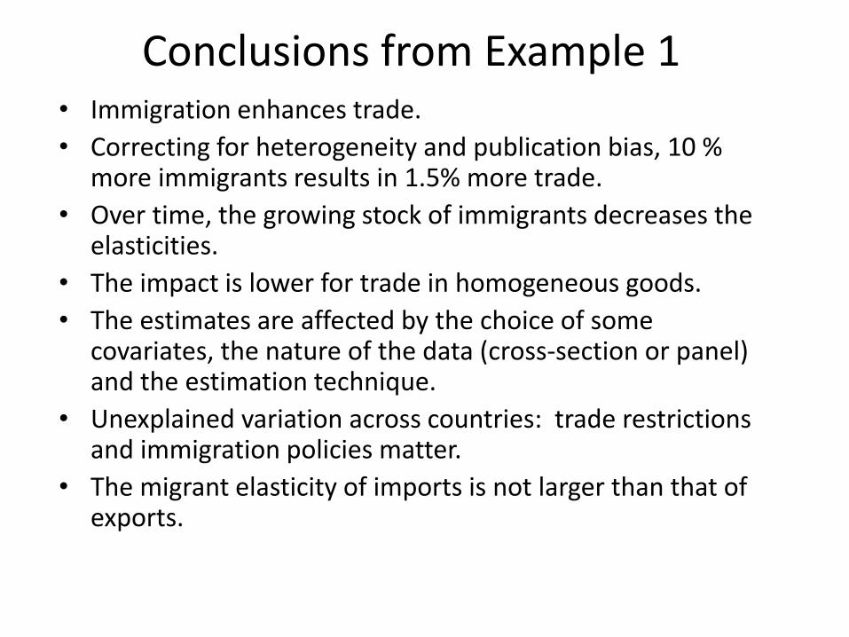
Conclusions from Example 1 • Immigration enhances trade.
• Correcting for heterogeneity and publication bias, 10 % more immigrants results in 1.5% more trade.
• Over time, the growing stock of immigrants decreases the elasticities.
• The impact is lower for trade in homogeneous goods.
• The estimates are affected by the choice of some covariates, the nature of the data (cross-section or panel) and the estimation technique.
• Unexplained variation across countries: trade restrictions and immigration policies matter.
• The migrant elasticity of imports is not larger than that of exports.
The big issues in meta-analysis
• Heterogeneity of effect sizes
• Heterogeneity of precision
• (Non)-experimental design and causality
• Selection bias and quality control
• Publication bias
• Clusters
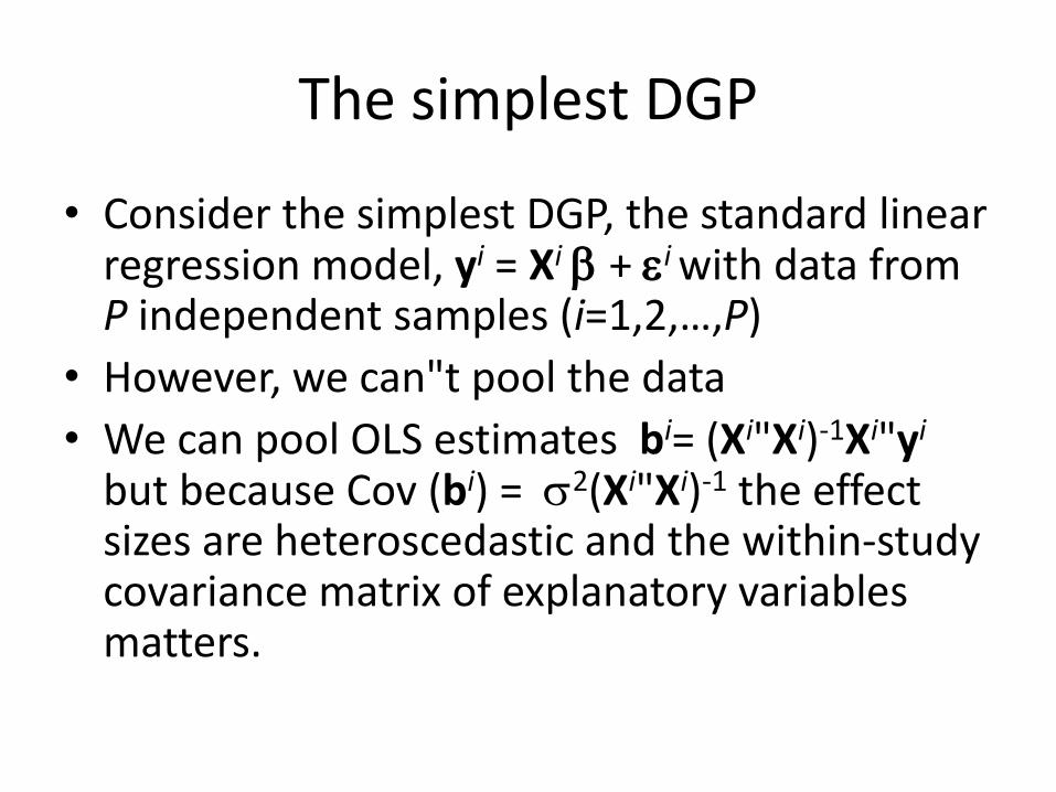
The simplest DGP
• Consider the simplest DGP, the standard linear regression model, yi = Xi + i with data from P independent samples (i=1,2,…,P)
• However, we can"t pool the data
• We can pool OLS estimates bi= (Xi"Xi)-1Xi"yi but because Cov (bi) = 2(Xi"Xi)-1 the effect sizes are heteroscedastic and the within-study covariance matrix of explanatory variables matters.
Heterogeneity, heteroscedasticity and bias
• In economics, will most likely differ between studies (heterogeneity). If so, we need to model this variation.
• Moreover, y and X vary across studies in sample size, definition of variables and selection of variables.
• Researchers also report various results of y and X variation within studies. Some of these results must be biased.
• Meta-sample selection also generates bias
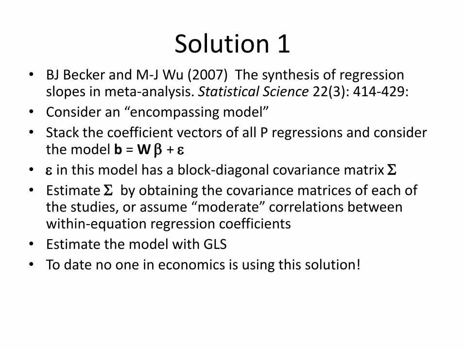
Solution 1 • BJ Becker and M-J Wu (2007) The synthesis of regression
slopes in meta-analysis. Statistical Science 22(3): 414-429:
• Consider an “encompassing model”
• Stack the coefficient vectors of all P regressions and consider the model b = W +
• in this model has a block-diagonal covariance matrix
• Estimate by obtaining the covariance matrices of each of the studies, or assume “moderate” correlations between within-equation regression coefficients
• Estimate the model with GLS
• To date no one in economics is using this solution!

Solution 2: The meta-regression model
• The generic form is
• The Mij are referred to as moderator variables that explain heterogeneity
• Clearly, the crucial issue is the DGP for i
• Various models have been proposed, of which the mixed effects model is the most popular (metareg in Stata)
iiKKiiiii MMMb ...22110
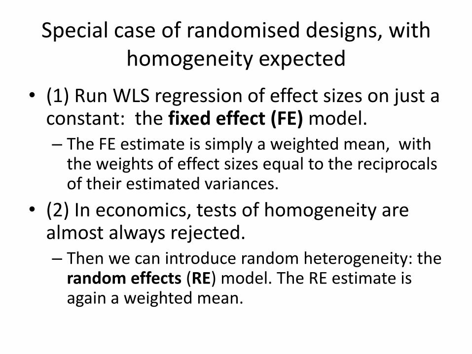
Special case of randomised designs, with homogeneity expected
• (1) Run WLS regression of effect sizes on just a constant: the fixed effect (FE) model. – The FE estimate is simply a weighted mean, with
the weights of effect sizes equal to the reciprocals of their estimated variances.
• (2) In economics, tests of homogeneity are almost always rejected. – Then we can introduce random heterogeneity: the
random effects (RE) model. The RE estimate is again a weighted mean.
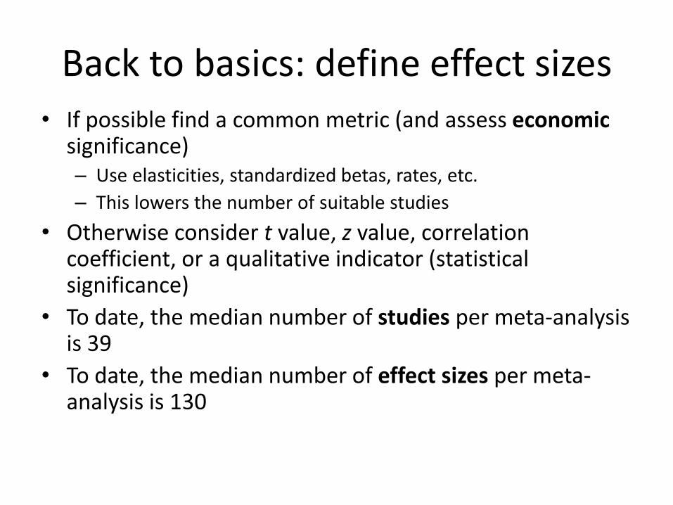
Back to basics: define effect sizes • If possible find a common metric (and assess economic
significance) – Use elasticities, standardized betas, rates, etc.
– This lowers the number of suitable studies
• Otherwise consider t value, z value, correlation coefficient, or a qualitative indicator (statistical significance)
• To date, the median number of studies per meta-analysis is 39
• To date, the median number of effect sizes per meta-analysis is 130

Create the data for meta-regression analysis
• Obtain studies that report the required effect sizes – Consider foreign language publications?
• Transform related estimates to effect sizes where possible
• Code all relevant study characteristics – Use theory to decide what matters
– Contact authors if needed
– Obtain relevant contextual information external to the study
• Have co-authors verify the coding
• Creating the dataset is the most costly part of meta-analysis
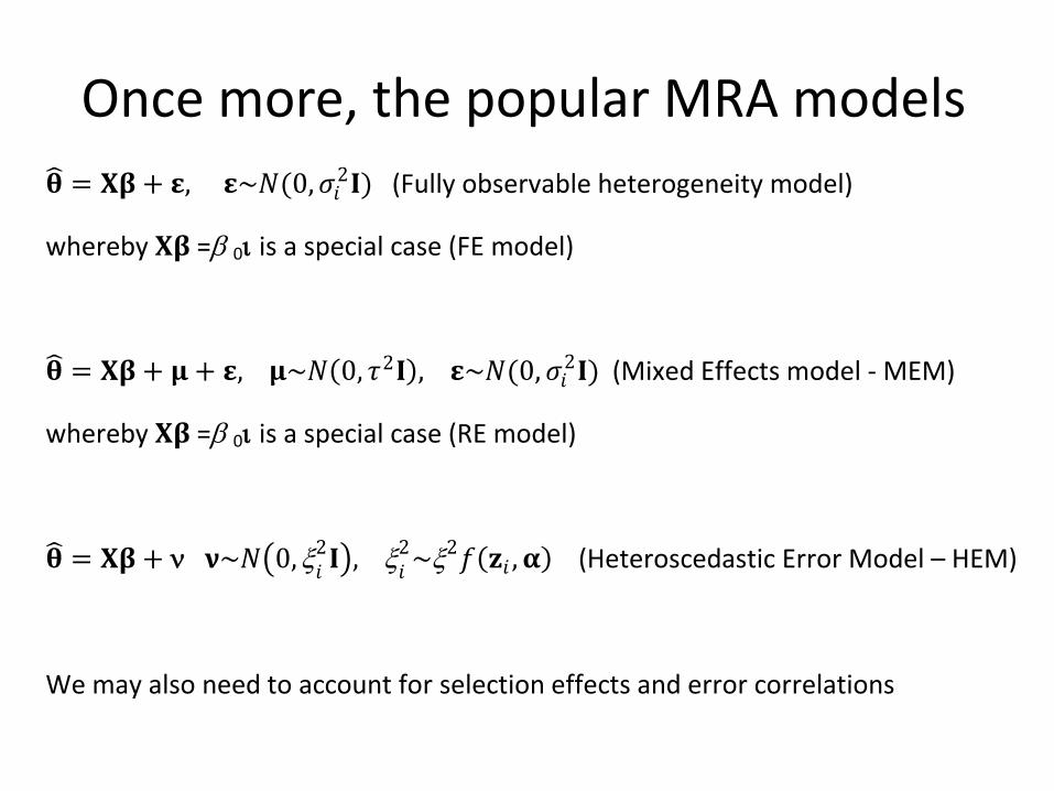
Once more, the popular MRA models
𝛉 = 𝐗𝛃 + 𝛆, 𝛆~𝑁(0,𝜎𝑖2𝐈) (Fully observable heterogeneity model)
whereby 𝐗𝛃 = 0 is a special case (FE model)
𝛉 = 𝐗𝛃 + 𝛍 + 𝛆, 𝛍~𝑁 0, 𝜏2𝐈 , 𝛆~𝑁(0, 𝜎𝑖2𝐈) (Mixed Effects model - MEM)
whereby 𝐗𝛃 = 0 is a special case (RE model)
𝛉 = 𝐗𝛃 + 𝛎~𝑁 0, 𝑖2𝐈 ,
𝑖2~2𝑓 𝐳𝑖 ,𝛂 (Heteroscedastic Error Model – HEM)
We may also need to account for selection effects and error correlations
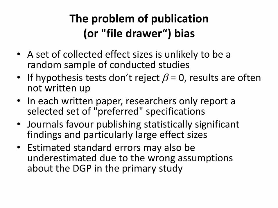
The problem of publication (or "file drawer“) bias
• A set of collected effect sizes is unlikely to be a random sample of conducted studies
• If hypothesis tests don’t reject = 0, results are often not written up
• In each written paper, researchers only report a selected set of "preferred" specifications
• Journals favour publishing statistically significant findings and particularly large effect sizes
• Estimated standard errors may also be underestimated due to the wrong assumptions about the DGP in the primary study

Example 2: The effect of the local unemployment rate on wages of individuals
• Since 1990, an inverse relationship between wages of individuals and local unemployment rates has been found for many countries, ln w = a – b ln U
• In their 1994 book, The Wage Curve, Blanchflower and Oswald argued that the unemployment elasticity of pay is around -0.1 in most countries.
• In a 1995 literature survey, Card referred to this striking empirical regularity as being close to an "empirical law of economics".
• Nijkamp P and Poot J (2005), The Last Word on the Wage Curve? Journal of Economic Surveys 19(3): 421-450, analysed 208 estimates with an average of -0.12
• Nonetheless, reported elasticities do vary widely, even excluding outliers, between about -0.5 and +0.1.

Evidence of publication bias in wage curve research
Data: 151 effect sizes from micro data used in 1 book and 16 refereed articles
ln root n
87654321
ln t
6
4
2
0
-2
-4
Simple publication bias test (Egger test): Regress t stat on 1/se with OLS: Slope is -0.057 (0.003) is measure of “true effect” Intercept is -2.214 (0.506) is measure of “publication bias”
0
50
010
00
invse
-1.5 -1 -.5 0Elasticity
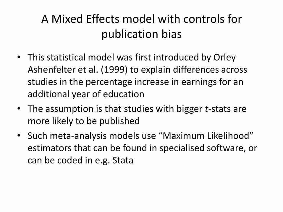
A Mixed Effects model with controls for publication bias
• This statistical model was first introduced by Orley Ashenfelter et al. (1999) to explain differences across studies in the percentage increase in earnings for an additional year of education
• The assumption is that studies with bigger t-stats are more likely to be published
• Such meta-analysis models use “Maximum Likelihood” estimators that can be found in specialised software, or can be coded in e.g. Stata
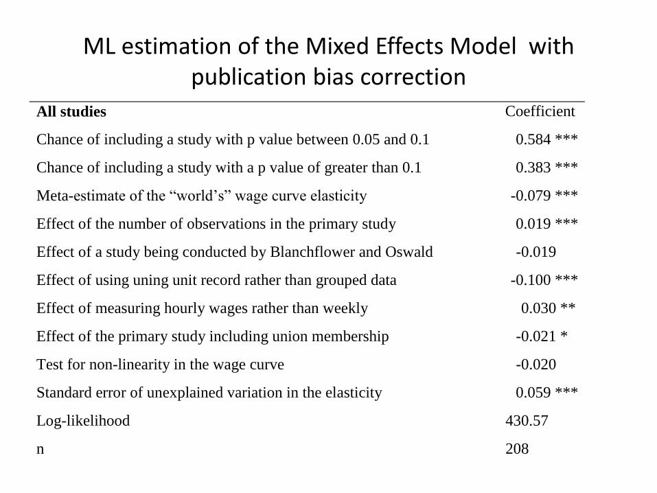
ML estimation of the Mixed Effects Model with publication bias correction
All studies Coefficient
Chance of including a study with p value between 0.05 and 0.1 0.584 ***
Chance of including a study with a p value of greater than 0.1 0.383 ***
Meta-estimate of the “world’s” wage curve elasticity -0.079 ***
Effect of the number of observations in the primary study 0.019 ***
Effect of a study being conducted by Blanchflower and Oswald -0.019
Effect of using uning unit record rather than grouped data -0.100 ***
Effect of measuring hourly wages rather than weekly 0.030 **
Effect of the primary study including union membership -0.021 *
Test for non-linearity in the wage curve -0.020
Standard error of unexplained variation in the elasticity 0.059 ***
Log-likelihood 430.57
n 208

Final example: The relationship between total savings in an
economy and age composition
• Purely macroeconomic perspective
• Seminal contribution:
Franco Modigliani"s “Life Cycle Hypothesis”: F. Modigliani
and R.E. Brumberg “Utility analysis and aggregate consumption functions”, mimeo, Carnegie-Mellon University, 1953.
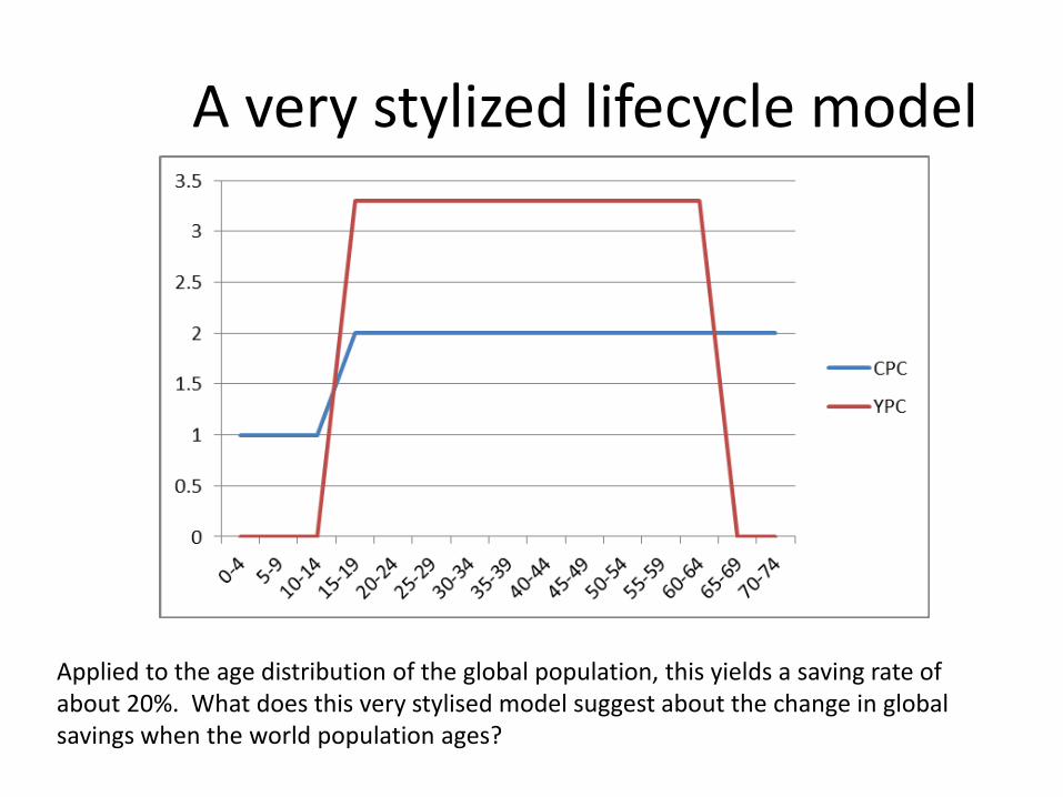
A very stylized lifecycle model
Applied to the age distribution of the global population, this yields a saving rate of about 20%. What does this very stylised model suggest about the change in global savings when the world population ages?
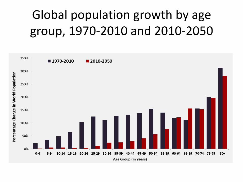
Global population growth by age group, 1970-2010 and 2010-2050
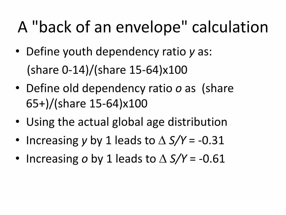
A "back of an envelope" calculation
• Define youth dependency ratio y as:
(share 0-14)/(share 15-64)x100
• Define old dependency ratio o as (share 65+)/(share 15-64)x100
• Using the actual global age distribution
• Increasing y by 1 leads to S/Y = -0.31
• Increasing o by 1 leads to S/Y = -0.61
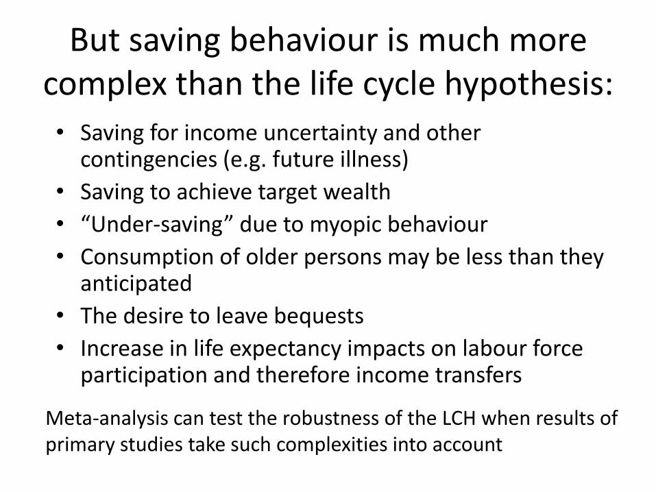
But saving behaviour is much more complex than the life cycle hypothesis: • Saving for income uncertainty and other
contingencies (e.g. future illness)
• Saving to achieve target wealth
• “Under-saving” due to myopic behaviour
• Consumption of older persons may be less than they anticipated
• The desire to leave bequests
• Increase in life expectancy impacts on labour force participation and therefore income transfers
Meta-analysis can test the robustness of the LCH when results of primary studies take such complexities into account
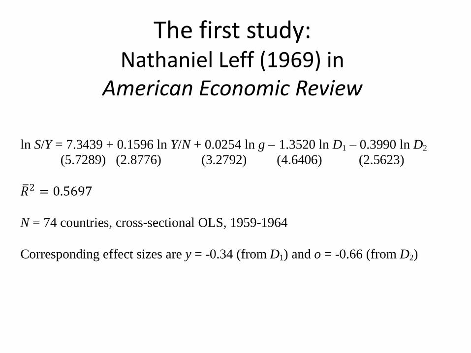
The first study: Nathaniel Leff (1969) in
American Economic Review
ln S/Y = 7.3439 + 0.1596 ln Y/N + 0.0254 ln g 1.3520 ln D1 – 0.3990 ln D2
(5.7289) (2.8776) (3.2792) (4.6406) (2.5623)
𝑅 2 = 0.5697 N = 74 countries, cross-sectional OLS, 1959-1964
Corresponding effect sizes are y = -0.34 (from D1) and o = -0.66 (from D2)

The distribution of a sample of 35 studies (1969-2007) with 316 effect sizes of the impact of
the child dependency ratio (y) and aged dependency ratio (o) on the aggregate saving rate
-3-2
-10
1
Qu
an
tile
s o
f O
0 .25 .5 .75 1Fraction of the data
-3-2
-10
1
Qu
an
tile
s o
f Y
0 .25 .5 .75 1Fraction of the data

Findings from meta-regression analysis (2012)
• Publication bias matters more in estimates in the effect of o than y
• Authors who assumed that the effect of y was the same as the effect of o found a smaller impact of LCH
• y has less impact on the national saving rate than the household saving rate; the opposite for o
• A one unit change in y has more impact on developed countries than on developing countries; the opposite for o
• y and o are themselves affected by the economy, (including savings). Authors that take this into account (through “IV estimation”) find bigger effects of y and o on savings.
• Authors who estimate dynamic models find smaller effects. • Authors who ignore the impact of variations in income per
capita and economic growth (i.e. they don’t estimate the Leff model or better) find biased effects.
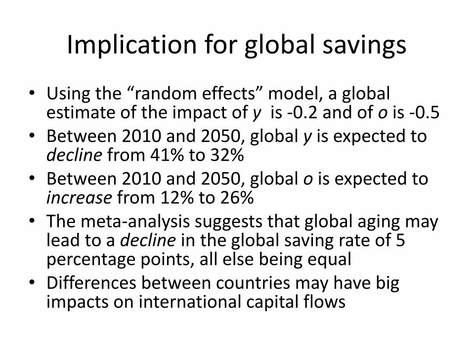
Implication for global savings
• Using the “random effects” model, a global estimate of the impact of y is -0.2 and of o is -0.5
• Between 2010 and 2050, global y is expected to decline from 41% to 32%
• Between 2010 and 2050, global o is expected to increase from 12% to 26%
• The meta-analysis suggests that global aging may lead to a decline in the global saving rate of 5 percentage points, all else being equal
• Differences between countries may have big impacts on international capital flows
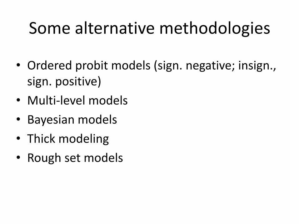
Some alternative methodologies
• Ordered probit models (sign. negative; insign., sign. positive)
• Multi-level models
• Bayesian models
• Thick modeling
• Rough set models
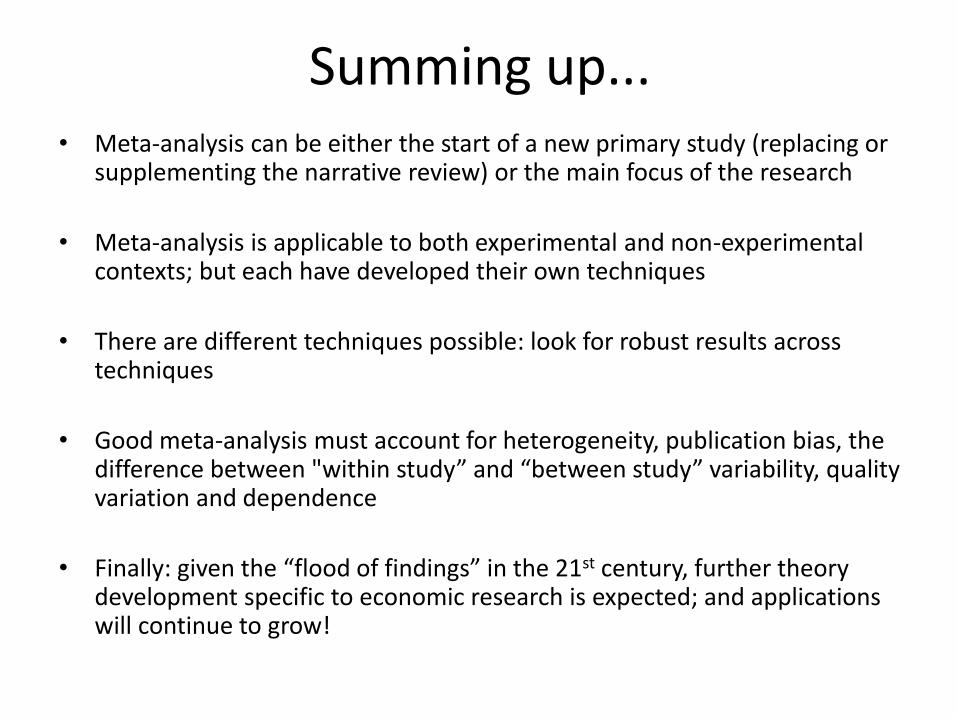
Summing up... • Meta-analysis can be either the start of a new primary study (replacing or
supplementing the narrative review) or the main focus of the research
• Meta-analysis is applicable to both experimental and non-experimental contexts; but each have developed their own techniques
• There are different techniques possible: look for robust results across techniques
• Good meta-analysis must account for heterogeneity, publication bias, the difference between "within study” and “between study” variability, quality variation and dependence
• Finally: given the “flood of findings” in the 21st century, further theory development specific to economic research is expected; and applications will continue to grow!