learning from patches by e cient spectral decomposition of

Mach Learn manuscript No.(will be inserted by the editor)

Learning from Patches by Efficient SpectralDecomposition of a Structured Kernel

Moshe Salhov · Amit Bermanis · GuyWolf · Amir Averbuch

Received: date / Accepted: date

Abstract We present a kernel based method that learns from a small neighbor-hoods (patches) of multidimensional data points. This method is based on spectraldecomposition of a large structured kernel accompanied by an out-of-sample ex-tension method. In many cases, the performance of a spectral based learning mech-anism is limited due to the use of a distance metric among the multidimensionaldata points in the kernel construction. Recently, different distance metrics havebeen proposed that are based on a spectral decomposition of an appropriate kernelprior to the application of learning mechanisms. The diffusion distance metric isa typical example where a distance metric is computed by incorporating the rela-tion of a single measurement to the entire input dataset. A method, which is calledPatch-to-Tensor Embedding (PTE), generalizes the diffusion distance metric thatincorporates matrix similarity relations into the kernel construction that replacesits scalar entries with matrices. The use of multidimensional similarities in PTEbased spectral decomposition results in a bigger kernel that significantly increasesits computational complexity. In this paper, we propose an efficient dictionaryconstruction that approximates the oversized PTE kernel and its associated spec-tral decomposition. It is supplemented by providing an out-of-sample extensionfor vector fields. Furthermore, the approximation error is analyzed and the advan-tages of the proposed dictionary construction are demonstrated on several imageprocessing tasks.

M. Salhov · A. Bermanis · G. Wolf · A. AverbuchSchool of Computer Science, Tel Aviv University, Tel Aviv 69978, IsraelM. SalhovE-mail: [email protected]. BermanisE-mail: [email protected]. Wolf.E-mail: [email protected]. AverbuchE-mail: [email protected]

2 Moshe Salhov et al.

1 Introduction

Recent machine learning methods for massive high dimensional data analysismodel observable parameters in such datasets by the application of nonlinear map-pings of a small number of underlying factors (Belkin and Niyogi 2003; Singer andCoifman 2008). Mathematically, these mappings are characterized by the geomet-ric structure of a low dimensional manifold that is immersed in a high dimensionalambient space. Under this model, the dataset is assumed to be sampled from anunknown manifold in the ambient observable space. Then, manifold learning meth-ods are applied to reveal the underlying geometry. Kernel methods such as k-PCA,Laplacian Eigenmaps (Belkin and Niyogi 2003) and Diffusion Maps (DM) (Coif-man and Lafon 2006) are designed for this task by utilizing the intrinsic manifoldgeometry. They have provided good results in representing and analyzing suchdata. Kernel methods are based on a scalar similarity measure between individualmultidimensional data points1.

In this paper, we describe a kernel construction when patches, which were takenfrom the underlying manifold, are analyzed instead of analyzing single data pointsfrom the manifold. Each patch is defined as a local neighborhood of a data pointin a dataset sampled from an underlying manifold. We focus on Patch-to-TensorEmbedding (PTE) kernel construction from (Salhov et al 2012) that is explainedlater. The relation between any two patches in a PTE based kernel constructionis described by a matrix that represents both the affinities between data pointsat the centers of these patches and the similarities between their local coordinatesystems. Then, the constructed matrices between all patches are combined into ablock matrix that is called super-kernel. This super-kernel is a non-scalar affinitykernel between patches (local neighborhood) of the underlaying manifold (Salhovet al 2012). The super-kernel is positive definite. It captures the intrinsic geometryof the underlying manifold/s. However, the proposed enhanced kernel increasesits size and hence, it increases the computational complexity of a direct spectraldecomposition of this kernel.

In this paper, we generalize the dictionary construction approach in (Engelet al 2004) to approximate the spectral decomposition of a non-scalar PTE basedkernel that utilizes the underlying patch structure inside the ambient space. Thecontributions of this paper are twofold:

1. We utilize the structure of the super-kernel from PTE to find a necessarycondition for updating a non-scalar based dictionary. This dictionary is usedto approximate the spectral decomposition of the super-kernel and to derive therequired conditions for achieving a bound on the super-kernel approximationerror. In addition, we analyze its computational complexity and estimate itsefficiency in comparison to the computation of a spectral decomposition of afull super-kernel.

2. We show how to efficiently extend the PTE embedding via an out-of-sampleextension to a newly arrived data point that did not participate in the dictio-nary construction. This includes the case when the analyzed dataset consistsof tangential vector fields and provides an out-of-sample extension method toprocess vector fields.

1 All the data points in this paper are multidimensional. They will be denoted as data points

Learning from Patches by Efficient Spectral Decomposition of a Structured Kernel 3

The PTE based kernel utilizes the Diffusion Maps (DM) methodology (Coif-man and Lafon 2006) that is described next. The DM kernel, which is based ona scalar similarity measure between individual data points, captures their connec-tivity. The kernel is represented by a graph where each data point correspondsto a vertex and the weight of an edge between any pair of vertices reflects thesimilarity between the corresponding data points. The analysis of the eigenvaluesand the corresponding eigenvectors of the kernel matrix reveals many proper-ties and connections in the graph. More specifically, the diffusion distance metric(Eq. 1) represents the transition probabilities of a Markov chain that advancesin time (Coifman and Lafon 2006). Unlike the geodesic distance or the shortestpath in a graph, the diffusion distance is robust to noise. The diffusion distancehas proved to be useful in clustering (David and Averbuch 2012), anomaly detec-tion (David 2009), parametrization of linear systems (Talmon et al 2012), shaperecognition (Bronstein and Bronstein 2011) to name some.

Formally, the original DM is used to analyze a dataset M by exploring thegeometry of the manifold M from which it is sampled. This method is based ondefining an isotropic kernel K ∈ Rn×n whose elements are defined by

k(x, y) , e−‖x−y‖2

ε , x, y ∈M, (1)

where ε is a meta-parameter of the algorithm that describes the kernel’s compu-tational neighborhood. This kernel represents the affinities between data points inthe manifold. The kernel is viewed as a construction of a weighted graph over thedataset M . Data points in M are the vertices and the weights (for example, wecan use the weight in Eq. 1) of the edges are defined by the kernel K. The degreeof each data point (i.e., vertex) x ∈ M in this graph is q(x) ,

∑y∈M

k(x, y). Nor-

malization of the kernel by this degree produces an n×n row stochastic transitionmatrix P whose elements are p(x, y) = k(x, y)/q(x), x, y ∈ M , which defines aMarkov process (i.e., a diffusion process) over the data points in M . A symmetricconjugate P of the transition operator P defines the diffusion affinities betweendata points by

p(x, y) =k(x, y)√q(x)q(y)

=√q(x)p(x, y)

1√q(y)

x, y ∈M. (2)

The DM method embeds a manifold into an Euclidean space whose dimensionalitymay be significantly lower than the original dimensionality. This embedding is aresult from the spectral analysis of the diffusion affinity kernel P . The eigenvalues1 = σ0 ≥ σ1 ≥ . . . of P and their corresponding eigenvectors φ0, φ1, . . . are usedto construct the desired map, which embeds each data point x ∈M into the datapoint Φ(x) = (σti φi(x))δi=0 for a sufficiently small δ, which is the dimension of theembedded space. The exact value of δ depends on the decay of the spectrum of P .

DM extends the classical Multi-Dimensional Scaling (MDS) core method (Coxand Cox 1994; Kruskal 1964) by considering nonlinear relations between datapoints instead of considering the original linear Gram matrix relations. Further-more, DM has been utilized for a wide variety data types and for pattern analysissuch as improving audio quality by suppressing transient interference (Talmon et al2013), detecting moving vehicles (Schclar et al 2010), scene classification (Jingen


et al 2009), gene expression analysis (Rui et al 2007), source localization (Talmonet al 2011) and fusion of different data sources (Lafon et al 2006; Keller et al 2010).

DM methodology is also used in finding both a parametrization and an explicitmetric, which reflects the intrinsic geometry of a given dataset. This is done byconsidering the entire pairwise connectivity between data points in a diffusionprocess (Lafon et al 2006).

Recently, DM has been extended in several directions to handle orientation inlocal tangent spaces (Singer and Wu 2011, 2012; Salhov et al 2012; Wolf and Aver-buch 2013). Under a manifold assumption, the relation between two local patchesof neighboring data points is described by a matrix instead of a scalar value.The resulting kernel captures enriched similarities between local structures in theunderlying manifold. These enriched similarities are used to analyze local areasaround data points instead of analyzing their specific individual locations. For ex-ample, this approach is beneficial in image processing for analyzing regions insteadof individual pixels or when data points are perturbed thus their surrounding areais more important than their specific individual positions. Since the constructionsof these similarities are based on local tangent spaces, they provide methods tomanipulate tangential vector fields. For example, they allow to perform an out-of-sample extension for vector fields. These manipulations are beneficial when theanalyzed data consists of directional information in addition to positional informa-tion on the manifold. For example, the goal in (Ballester et al 2001) is to recovermissing data in images while utilizing interpolation of the appropriate vector field.Another example is in the utilization of tangential vector fields interpolation on S2

for modeling atmospheric air flow and oceanic water velocity (Fuselier and Wright2009).

The main motivation of this paper is to show the beneficial aspects in us-ing PTE based construction while reducing its computational complexity whenspectral decomposition of a PTE based kernel is used.

The spectral decomposition computational complexity can be reduced in sev-eral ways. Kernel matrix sparsification is a widely used approach that utilizes asparse eigensolver such as Lanczos to compute the relevant eigenvectors (Cullumand Willoughby 2002). Another sparsification approach is to translate the densesimilarity matrix into a sparse matrix by selectively truncating elements outsidea given neighborhood radius of each data point. More sparsification approachesare given in (von Luxburg 2007). An alternative approach to reduce the compu-tational complexity is based on Nystrom extension for estimating the requiredeigenvectors (Fowlkes et al 2004). The Nystrom based method has three steps: 1.The given dataset is subsampled uniformly over its indices set. 2. The subsamplesdefine a kernel that is smaller than the dataset size. Then, the corresponding spec-tral decomposition is achieved by the application of a SVD solver to this kernel.3, The solution of the small spectral problem is extended to the entire datasetvia the application of Nystrom extension method. The result is an approximatedspectral method. Although this solution is much more computationally efficientthan the application of the spectral decomposition to the original kernel matrix,the resulting approximated spectral method suffers from several major problemsoriginated from the subsampling effect on the spectral approximation and fromthe ill-conditioned effects in the Nystrom extension method.

Recently, a novel multiscale scheme is suggested in (Bermanis et al 2013) forsampling scattered data and for extending functions defined on sampled data


points. The suggested approach, also called Multiscale Extension (MSE), over-comes some limitations of the Nystrom method. For example, it overcomes theill-conditioned effect in the Nystrom extension method and accelerates the com-putation. The MSE method is based on mutual distances between data points. Ituses a coarse-to-fine hierarchy of a multiscale decomposition of a Gaussian kernel.Another interesting approach is suggested in (Engel et al 2004) to identify a subsetof data points (called dictionary) and a corresponding extension coefficients thatenable us to approximate the full scalar kernel. The number of dictionary atoms de-pends on the given data, kernel configuration and on the designed parameter thatcontrols the quality of the full kernel approximation. These are efficient methodsdesigned to process general kernels. However, they are not designed to utilize andpreserve the inherent structure that resides in kernels such as a super-kernel (Sal-hov et al 2012).

In summary, methods such as Nystrom and kernel recursive least squares,to name some, have been suggested to approximate large kernels decomposition.However, none of the suggested methods utilize the inherent structure of the PTEkernel nor suggest an out-of-sample extension method for vector fields. In thispaper, we propose a dictionary construction that approximates the oversized PTEkernel and its associated spectral decomposition. Furthermore, the approximationerror is analyzed and the advantages of the proposed dictionary construction aredemonstrated on a several image processing tasks.

The paper has the following structure: Section 2 formulates the problem. ThePatch-to-Tensor Embedding is described in section 3. The patch-based dictionaryconstruction and its properties are described in section 4. Finally, section 5 de-scribes the experimental results for image segmentation and for handwritten digitclassification that are based on the utilization of a dictionary-based analysis.

2 Problem Formulation

In this paper, we approximate the spectral decomposition of a large and structuredkernel. We assume that we have a dataset of n multidimensional data points thatare sampled from a manifoldM that lies in the ambient space Rm. We also assumethat the intrinsic dimension ofM is d m. We consider two related tasks: 1. Howto approximate the spectral decomposition of a super-kernel? This is explained insection 2.2. 2. How to perform an out-of-sample extension for vector fields? Thisis explained in section 2.3.

2.1 Manifold Setup

At every multidimensional data point x ∈ M , the manifold has a d-dimensionaltangent space Tx(M), which is a subspace of Rm. We assume that the manifold isdensely sampled thus, the tangential space Tx(M) can be approximated by a smallenough patch (i.e., neighborhood) N(x) ⊆M around x ∈M . Let o1x, . . . , o

dx ∈ Rm,

where oix = (oi,1x , . . . , oi,mx )T , i = 1, . . . , d, form an orthonormal basis of Tx(M)


and let Ox ∈ Rm×d be a matrix whose columns are these vectors

Ox ,

| | |o1x · · · oix · · · odx| | |

x ∈M. (3)

The matrix Ox can be analyzed spectrally by using a local PCA method (Singerand Wu 2011). We do it differently. From now on we assume that the vectorsin Tx(M) are expressed by their d coordinates according to the basis o1x, . . . , o

dx.

For each vector u ∈ Tx(M), the vector u = Oxu ∈ Rm is the same vector asu represented by m coordinates, according to the basis of the ambient space. Foreach vector v ∈ Rm in the ambient space, the vector v′ = OTx v ∈ Tx(M) is a linearprojection of v on the tangent space Tx(M). This setting was used in (Salhov et al2012).

In section 2.2, we formulate the spectral decomposition problem.

2.2 Approximation of the Super-Kernel Spectral Decomposition

The super-kernel G, which is constructed in (Salhov et al 2012), on a dataset M ,is based on the d orthonormal basis vectors in each Ox, x ∈ M . G is a nd × ndstructured matrix. Each d × d block in G is a similarity-index matrix between apair of data points and their corresponding neighborhoods. More details of thestructure of G are given in Section 3 (specifically, in Definition 1). Given a datasetM , the PTE method (Salhov et al 2012) uses the spectral decomposition of G toembed each data point (or neighborhood around it) to a tensor. This embedding iscomputed by constructing the coordinate matrices of the embedded tensors usingthe eigenvalues and the eigenvectors of G.

We want to efficiently approximate the PTE embedded tensors without com-puting directly the spectral decomposition of G. Under the manifold assumption,the super-kernel G has a small number of significant singular values in comparisonwith the dimensionality m of the given data. Hence, a low rank approximation ofthe super-kernelG exists. We aim to find a dictionaryDηn of ηn representative datapoints that will be used to construct a small super-kernel Gn and a correspondingextension matrix En ∈ Rηnd×nd that approximates the entire super-kernel G by

G ≈ ETn GnEn. (4)

The approximation of the spectral decomposition of G is computed by the appli-cation of QR decomposition (see (Golub and Van Loan 2012), page 246) to En. Inorder to construct a dictionary of representatives, we design a criterion that willidentify data points and their corresponding embedded tensors that are approxi-mately linearly independent. This criterion is utilized to control the approximationerror bound.

2.3 Out-of-Sample Extension Method for Vector Fields

Consider a tangential vector field v : M → Rd such that for all x ∈ M , v(x) ∈

Tx(M). The goal is to find an out-of-sample extension method for such tangential


vector fields. More specifically, given a new data point on the manifold, we aim tofind the vector in its local tangential space that corresponds smoothly to the knownvalues of the vector field. This out-of-sample extension method is used to extendthe coordinate matrices of the embedded tensors of PTE and to approximate theembedding of a new data point x /∈M .

A tangential vector field can be technically described in two forms. The stan-dard intuitive form describes it as a set of separate vectors or, equivalently, as an× d matrix whose rows are these vectors. An alternative form is to concatenateits tangential vectors to represent the vector field by vector of length nd. Figure 1illustrates these two forms.

v as a matrix in Rn×d n rows

v(x1)

.

..v(xn)

︸︷︷︸

d columns

n rows

v as a vector in Rnd n subvectors

d cells

d cells

|v(x1)|

...

|v(xn)|

nd cells

Fig. 1 x1, . . . , xn are used here to denote all the data points in M . Top: A viewing illustrationof a vector field v : M → Rd as a n× d matrix. Bottom: A vector of length nd.

Let x′ ∈ M\M be a new data point with the matrix Ox′ whose columnso1x′ , . . . , o

dx′ form an orthonormal basis for the tangential space Tx′(M). The out-

of-sample extension problem is formulated as finding an extension vector field uthat enables us to compute a vector v(x′) for any new data point x′.

The super-kernel G defines an integral operator on tangential vector fields onthe manifold M that are restricted to the dataset M (see (Wolf and Averbuch2013, Definition 4.1)). This integral operator can be formally described by theapplication of a super-kernel matrix to a long-vector (second representation form)that represents vector fields. By abuse of notation, if we treat u as its vector rep-resentation in Rnd, we define the relation between u and v(x′) using the operatorG to be

v(x′) ,∑y∈M

G(x′,y)u(y), (5)

where G(x′,y) are the non-scalar similarity blocks between the new data pointx′ /∈M and the data points y ∈M . We will use Eq. 5 to provide an interpolationscheme for finding the described vector field u and for using it for the out-of-sample


extension of tangential vector fields in general and for the PTE based embeddedtensors in particular. The latter is achieved by extending the eigenvectors of G,which are vectors in Rnd that are regarded as tangential vector fields.

3 Patch-to-Tensor Embedding

In this section, we review the main results from (Salhov et al 2012; Wolf andAverbuch 2013) regarding the super-kernel in order to make the entire presentationself contained.

3.1 Linear-Projection Diffusion Super-Kernel

For x, y ∈ M , define Oxy = OTxOy ∈ Rd×d, where Ox and Oy were definedin Eq. 3. The matrices Ox and Oy represent the bases for the tangential spacesTx(M) and Ty(M), respectively. Thus, the matrix Oxy, which will be referred toas the tangential similarity matrix, represents a linear-projection between thesetangential spaces. According to (Salhov et al 2012; Wolf and Averbuch 2013), thislinear-projection quantifies the similarity between these tangential spaces via theangle between their relative orientations.

Let Ω ∈ Rn×n be a symmetric and positive semi-definite affinity kernel definedon M ⊆ Rm. Each row or each column in Ω corresponds to a data point in M , andeach element [Ω]xy = ω(x, y), x, y ∈ M , represents the affinity between x and y,thus, ω(x, y) ≥ 0 for every x, y ∈M . The diffusion affinity kernel is an example forsuch an affinity kernel. Definition 1 uses the tangent similarity matrices and theaffinity kernel Ω to define the Linear-Projection super-kernel. When the diffusionaffinities in P (Eq. 2) are used instead of using the general affinities in Ω, thenthis structured kernel is called a Linear-Projection Diffusion (LPD) super-kernel.

Definition 1 (Salhov et al 2012)[Linear-Projection Diffusion Super-Kernel] ALinear-Projection Diffusion (LPD) super-kernel is a block matrix G ∈ Rnd×ndof size n× n where each block in it is a d× d matrix. Each row and each columnof blocks in G correspond to a data point in M . A single block G(x,y), x, y ∈ M ,represents an affinity (similarity) between the patches N(x) and N(y). Each blockG(x,y) ∈ Rd×d of G is defined as G(x,y) , p(x, y)Oxy = a(x, y)OTxOy, x, y ∈M .

The super-kernel in Definition 1 encompasses both the diffusion affinities be-tween data points from the manifoldM and the similarities between their tangen-tial spaces. The latter are expressed by the linear-projection operators betweentangential spaces. Specifically, for two tangential spaces Tx(M) and Ty(M) atx, y ∈M of the manifold, the operator OTxOy (i.e., their tangential similarity ma-trix) expresses a linear projection from Ty(M) to Tx(M) via the ambient spaceRm. The obvious extreme cases are the identity matrix, which indicates the ex-

istence of a complete similarity, and a zero matrix, which indicates the existenceof orthogonality (i.e., a complete dissimilarity). These linear projection operatorsexpress some important properties of the manifold structure, e.g., curvatures be-tween patches and differences in orientation. More details on the properties of thissuper-kernel are given in (Salhov et al 2012; Wolf and Averbuch 2013).


It is convenient to use the vectors oix and ojy to apply a double-indexing scheme

by using the notation g(oix, ojy) , [G(x,y)]ij that considers each single cell in G as

an element [G(x,y)]ij , 1 ≤ i, j ≤ d, in the block G(x,y), x, y ∈ M . It is important

to note that g(oix, ojy) is only a convenient notation and a single element of a block

in G does not necessarily have any special meaning. The block itself, as a whole,holds meaningful similarity information.

Spectral decomposition is used to analyze the super-kernel G. It is utilized toembed the patches N(x), x ∈ M , in a manifold, into a tensor space. Let |λ1| ≥|λ2| ≥ . . . ≥ |λ`| be the ` most significant eigenvalues of G and let φ1, φ2, . . . , φ`be their corresponding eigenvectors. Each eigenvector φi, i = 1, . . . , `, is a vectorof length nd. We denote each of its elements by φi(o

jx), x ∈ M , j = 1, . . . , d. An

eigenvector φi is a vector of n blocks, each of which is a vector of length d thatcorresponds to a data point x ∈ M on the manifold. To express this notion, weuse the notation ϕji (x) = φi(o

jx). Thus, the block, which corresponds to x ∈M in

φi, is the vector (ϕ1i (x), . . . , ϕdi (x))T .

The eigenvalues and the eigenvectors of G are used to construct a spectral map

Φ(ojx) = (λt1φ1(ojx), . . . , λt`φ`(ojx)), (6)

which is similar to the one used in DM and t is the diffusion transition time. Thisspectral map is then used to construct the embedded tensor Tx ∈ R`⊗Rd for eachx ∈M . These tensors are represented by the `× d matrices

Tx ,

| |Φ(o1x) · · · Φ(odx)| |

x ∈M. (7)

In other words, the coordinates of Tx (i.e., the elements in this matrix) are [Tx]ij =λtiϕ

ji (x), i = 1, . . . , `, j = 1, . . . , d. Each tensor Tx represents an embedding of the

patch N(x), x ∈M , into the tensor space R` ⊗Rd.The computational complexity of the direct spectral decomposition of a super-

kernel is in the order of O(n3d3

). However, the structure of the super-kernel can

be utilized for simplifying the decomposition. The super kernel can be viewedas the Khatri-Rao product (Rao 1968) of the diffusion affinity matrix Ω withthe nd × nd matrix B = OOT , where the matrix O ∈ Rnd×d is a block ma-trix with OTi as its d × d ith subblock. Hence, let G = Ω B be the corre-sponding Khatri-Rao product where the blocks of Ω are the affinity scalars andthe blocks of B are the d × d respected matrices OTi Oj . It can be shown thatthe symmetric partition of B can be used to reformulate the Khatri-Rao prod-uct in terms of a Kronecker product as G = Z (Ω ∗B)ZT , where Z is a propernd × n2d2 selection matrix (Liu and Trenkler 2008), ZTZ = I and Ω ∗ B isthe Kronecker product of Ω and B. Let Ω = UΩΣΩV

TΩ be the SVD of Ω and

B = UBΣBVTB be the SVD of B, then the spectral decomposition of G can be

reformulated using the spectral decomposition characterization of a Kroneckerproducts as G = UΣV = Z (UΩ ∗ UB) (ΣΩ ∗ΣB) (VΩ ∗ VB)ZT . Hence, the com-putation of the left eigenvectors U = Z (UΩ ∗ UB) requires O

(n3)

operations todecompose Ω and additional operations that are needed for the decomposition ofO. The total computational cost is more efficient than what is needed to decom-pose nd×nd super-kernel. However, computational cost of O

(n3)

to process largedatasets is impractical. Hence, we are looking for a reduction of at least one orderof magnitude in the spectral decomposition of large matrices.


4 Patch-Based Dictionary Construction

According to Lemma 3.3 in (Salhov et al 2012), the sum in Eq. 5 can be rephrasedin terms of the embedded tensors x ∈M to be

v(x) =∑y∈M

T Tx Tyu(y). (8)

However, due to linear dependencies between the embedded tensors, this sum maycontain redundant terms. Indeed, if a tensor Tz can be estimated as a weightedsum of other tensors as Tz =

∑z 6=y∈M CzyTy, where Czy ∈ R, z 6= y ∈ M are the

scalar weights that relates a tensor Tz to any other tensor Ty. Now, Eq. 8 becomesfor x ∈M

v(x) =∑

z 6=y∈M

T Tx Ty(u(y) + Czyu(z)). (9)

This enables us to eliminate the redundant tensors. By applying an iterative ap-proach, we obtain a small subset of tensors, which is a set of linearly independenttensors that are sufficient to compute Eqs. 8 and 5.

Similarly, we can use the matrix coefficients Czy ∈ Rd×d instead of individualscalars to incorporate more detailed relations between the tensor Tz and any ten-sors Ty. Therefore, Tz is tensorialy dependent in Tyz 6=y∈M if it satisfies for somematrix coefficients Czy

Tz =∑

z 6=y∈M

TyCzy . (10)

The defined dependency described in Eq. 9 expresses more redundancies thanwhat a standard linear dependency expresses. As a result, we obtain a sparse setof independent tensors that enables us to efficiently compute Eqs. 8 and 5. Thisset of representative tensors constitutes a dictionary that represents the embeddedtensor space.

4.1 Dictionary Construction

We use an iterative approach to construct the described dictionary by one sequen-tial scan of the entire data points in M . In the first iteration, we define the scannedset to be X1 = x1 and the dictionary D1 = x1. At each iteration s = 2, . . . , n,we have a new data point xs, the scanned set Xs−1 = x1, . . . , xs−1 from theprevious iteration and the dictionary Ds−1 that represents Xs−1. The dictionaryDs−1 is in fact a subset of ηs−1 data points from Xs−1 that are sufficient to repre-sent its embedded tensors. We define the scanned set Xs = Xs−1∪xs. Our goalis to define the dictionary Ds of Xs based on the dictionary Ds−1 with the newdata point xs. To do this, a dependency criterion has to be established. If this cri-terion is satisfied, then the the dictionary remains the same such that Ds = Ds−1.Otherwise, it is updated to include the new data point Ds = Ds−1 ∪ xs.

We use a dependency criterion that is similar to the approximated linear de-pendency (ALD) criterion used in KRLS (Engel et al 2004). The ALD measuresthe distance between candidates vector and the span by the dictionary vectors,to determine if the dictionary should be updated. In our case, we want to ap-proximate the tensorial dependency (Eq. 10) of the examined tensor Txs with the


tensors in the dictionary Ds−1. Therefore, we define the distance of Txs from thedictionary Ds−1 by

δs , minCs1 ,...,C

sηs−1

∥∥∥∥∥∥ηs−1∑j=1

TyjCsj − Txs

∥∥∥∥∥∥2

F

, Cs1 , . . . , Csηs−1

∈ Rd×d, (11)

where ‖·‖F denotes the Frobenius norm and Cs1 , . . . , Csηs−1

are the matrix coeffi-cients in Eq. 10. We define the approximated tensorial dependency (ATD) criterionto be δs ≤ µ, for some accuracy threshold µ > 0. If the ATD criterion is satis-fied, then the tensor Txs can be approximated by the dictionary Ds−1 using thematrix coefficients Cs1 , . . . , C

sηs−1

that achieve the minimum in Eq. 11. Otherwise,the dictionary has to be updated by adding xs to it.

Lemma 1 Let Gs−1 ∈ Rdηs−1×dηs−1 be a super-kernel of the data points in thedictionary Ds−1 and let Hs ∈ Rdηs−1×d be a ηs−1 × 1 block matrix whose j-thd × d block is G(yj ,xs), j = 1, . . . , ηs−1. Then, the optimal matrix coefficients(from Eq. 11) are Csj , j = 1, . . . , ηs−1, where Csj is the j-th d × d block of the

ηs−1 × 1 of d × d blocks matrix G−1s−1Hs. The corresponding error δs in Eq. 11

satisfies δs = tr[G(xs,xs) −HTs G−1s−1Hs].

Proof The minimizer in Eq. 11 is rephrased as

δs = minCs1 ,...,C

sηs−1

tr

ηs−1∑j=1

TyjCsj − Txs

T ηs−1∑j=1

TyjCsj − Txs

.

Algebraic simplifications yield

δs = minCs1 ,...,C

sηs−1

tr

ηs−1∑i=1

ηs−1∑j=1

CsiTT Tyi TyjC

sj −

ηs−1∑j=1

T TxsTyjCsj

−ηs−1∑j=1

CsjTT Tyj Txs + T TxsTxs

.

The products between the embedded tensors (e.g., T Tyj Txs , j = 1, . . . , ηs−1) canbe replaced with the corresponding super-kernel blocks via Lemma 3.3 in (Salhovet al 2012). We perform these substitutions and get

δs = minA

tr[AT Gs−1A−HT

s A−ATHs +G(xs,xs)

], (12)

where A ∈ Rdηs−1×d is a ηs−1 × 1 block matrix whose j-th d × d block is Csj ,j = 1, . . . , ηs−1. Solving the optimization (i.e., minimization) in Eq. 12 yields thesolution

As = G−1s−1Hs, (13)

that proves the lemma.


Lemma 1 provides an expression for a dictionary-based approximation in super-kernel terms. Essentially, this eliminates the need for prior knowledge of the em-bedded tensors during the dictionary construction. At each iteration s, we considerthe criterion δs < µ. Based on this condition, we decide whether to add xs to thedictionary or just to approximate its tensor. The threshold µ is given anywayin advance as a meta-parameter and δs is computed by using the expression inLemma 1, which does not depend on the embedded tensors. Therefore, the dic-tionary construction process only requires knowledge of the super-kernel blocksthat are needed to compute this expression in every iteration. In fact, the numberof required blocks is relatively limited since it is determined by the size of thedictionary and not by the size of the dataset.

4.2 The Dictionary Construction Algorithm

In this section, we specify the steps that take place in each iteration s in thedictionary construction algorithm. Let Es be a (ηs × d)× (s× d) block matrix atiteration s whose (i, j) entry (block) is the optimal coefficient matrix Cji , 1 ≤ i ≤ηs, 1 ≤ j ≤ s computed in Lemma 1. The coefficient matrix Cji has two solutionsthat depend on the ATD criterion calculated in iteration s. First, Lemma 1 isapplied to compute δs. Then, two possible scenarios are considered:

1. δs ≤ µ, hence, Txs (Eq. 7) satisfies the ATD on Ds−1. The dictionary re-mains the same, i.e., Ds = Ds−1 and Gs = Gs−1. The extension matrixEs = [Es−1 As] is computed by concatenating the matrix As = G−1

s−1Hs (fromthe proof of Lemma 1) with the coefficient matrix from the previous iterations− 1.

2. δs > µ, hence, Txs does not satisfy the ATD on Ds−1. The vector xs is addedto the dictionary, i.e., Ds = Ds−1 ∪ xs. The computation of Es is done byadding the identity matrix and the zero matrix in the appropriate places. Thedictionary related super-kernel Gs becomes

Gs =

[Gs−1 HsHTs G(xs,xs)

]. (14)

The computation of the ATD conditions during these iterations requires to haveG−1s of the dictionary based super-kernels. The block matrix inversion in Eq. 14

becomes

G−1s =

[G−1s−1 +As∆−1

s (As)T −As∆−1s

−∆−1s (As)T ∆−1

s

], (15)

where ∆s = G(xs,xs) − HTs G−1s−1Hs is computed through the applicability of the

ATD test.At each iteration s, the PTE of the data points Xs (or, more accurately, their

patches) is based on the spectral decomposition of the super-kernel Gs of Xs. Thisspectral decomposition is approximated by using the extension matrix Es and thedictionary related super-kernel Gs (Eq. 14).

Let ETs = QsRs be the QR decomposition of this extension matrix, whereQs ∈ Rds×dηs is an orthogonal matrix and Rs ∈ Rdηs×dηs is the upper triangularmatrix. Additionally, let RsGsR

Ts = UsΣsU

Ts be the SVD of RsGsR

Ts . Then,


the SVD of ETs GsEs is ETs GsEs = (QsUs)ΣsQTs U

Ts . Thus, the SVD of Gs is

approximated by Gs ≈ UsΣsUTs , where

Us = QsUs. (16)

The dictionary construction followed by the patch-to-tensor embedding ap-proximation process is described in Algorithm 4.1.

Algorithm 4.1: Patch-to-Tensor Dictionary Construction and EmbeddingApproximation (PTEA)

Input: Data points: x1, ..., xn ∈ Rm and their corresponding localtangential basis Oxi , i = 1, . . . , n.Parameters: Max approximation tolerance µ, tensor of length ` and

dataset of size nOutput: The Estimated Tensors Txi , i = 1, . . . , n, the extension matrix En

and the super-kernel Gn1: Initialize: G1 = G(x1,x1) (block, definition 1), G−1

1 = G−1(x1,x1)

, E1 = Id,

D1 = x1, η1 = 12: for s = 2 to n do

Compute Hs =[G(x1,xs), ..., G(Xηs ,xs)

]ATD Test:

Compute As = G−1s−1Hs

Compute ∆ = G(xs,xs) −HTs As

Compute δ = tr[∆]If δ < µ

Set Es =[Es−1 As

]Set Ds = Ds−1

Else (update dictionary)

Set Es =

[Es−1 0

0 Id

]Set Ds = Ds−1 ∪ xsUpdate Gs according to Eq. 14Update G−1

s according to Eq. 15Set ηs = ηs−1 + 1

3: Approximate Un according Eq. 16.4: Use Un to compute the approximated spectral map Φ(ojx), x ∈M ,j = 1, . . . , d, according to Eq. 6 (considering the first ` eigenvalues and thecorresponding eigenvectors).

5: Use the spectral map Φ to construct the tensors Tx ∈ R` ⊗Rd, x ∈M ,according to Eq. 7.

The computational complexity of Algorithm 4.1 is given in Table 1. When nηn, the computational complexity O(nd3η2n) from the application of the proposedmethod is substantially lower than the computational complexity O(d3n3) fromthe application of the straightforward SVD.


Table 1 PTEA Computational Cost

Operation CostCompute δs O(η2sd

3)

Update Gs,Es and G−1s O(η2sd

3)QR of Es O(sη2sd

2)

SVD of RsGsRTs O(η3sd3)

QsUs to approximate Txi O(sη2sd3)

4.3 The Super-Kernel Approximation Error Bound

The dictionary construction allows us to approximate the entire super-kernel with-out direct computation of every block in it. Given the dictionary constructionproduct Es, then the super-kernel Gs of the data points in Xs is approximated by

Gs ≈ ETs GsEs, (17)

where Gs ∈ Rηsd×ηsd is the super-kernel of the data points in the dictionary Ds.

For the quantification of Eq. 17, let Ψs∆= [Tx1 , ..., Txs ] be the ` × sd matrix

that aggregates all the embedded tensors up to a step s, where Txi ∈ Rl×d,

i = 1, . . . , s. Let Ψs∆= [Ty1 , ..., Tyηs ] be the ` × ηsd matrix that aggregates all

the embedded tensors of the dictionary members Ds and let Ψ ress , Ψs − ΨsEs =

[ψres1 , . . . , ψres

s ], where ψress , Txs −

∑ηs−1

j=1 TyjCsj . Then, due to Eq. 11 and the

ATD condition, ‖Ψ ress ‖2F ≤ sµ. From Definition 1 of the super-kernel, we get

Gs = ΨTs Ψs and Gs = ΨTs Ψs. Therefore, by substituting Ψs into Eq. 17 we getGs = EsGsE

Ts +(Ψ res

s )TΨ ress where all the cross terms vanish by the optimality of

Es. As a consequence, the approximation error Rs = Gs−EsGsETs = (Ψ ress )TΨ res

s

in step s satisfies ‖Rs‖2F ≤ sµ. In particular, for s = n, ‖Rn‖2F ≤ nµ.

4.4 Out-of-Sample Extension for Vector Fields

The presented dictionary estimates a tangential vector field by using a recursivealgorithm similar to the well known Kernel Recursive Least Squares (KRLS) (En-gel et al 2004). In a supervised learning scheme, the predictor in Eq. 5 is designedto minimize the l2 distance between the predicted vector field at each iteration sand the actual given vector field (as part of the training set) by

J(w) =s∑i=1

‖ν(xi)−ν(xi)‖22 =s∑i=1

∥∥∥∥∥∥t∑

j=1

G(xi,xj)wj − ν(xi)

∥∥∥∥∥∥2

2

= ‖Gw−ν‖22, (18)

where w is the predictor weights vector and ν is the concatenation of all thegiven training values of the vector field2. The Recursive Least Squares solution,which minimizes J(w), is given by wo = G−1ν. In the case when the number ofvector examples is large, the complexity of inverting the super-kernel tends to beexpensive in terms of computational cost and memory requirements. Furthermore,

2 For the sake of simplicity, we use this slight abuse of notation. Namely, the same notationis used for the vector field and for the aggregation of its known values.


the length of the predictor weight vector wo depends on the number of trainingsamples. Hence, redundant samples, which generate linearly-dependent rows in thesuper-kernel, will generate over fitting by the predictor. One possible remedy forthese problems is to utilize the sparsification procedure from Section 4.2 in order todesign the predictor. The optimizer wo is formulated by introducing the dictionaryestimated super-kernel as J(w) = ‖Gw − ν‖22 ≈ ‖ETs GsEsw − ν‖22 as in Eq. 17.Let α = Esw, then the predictor is reformulated as ν(xi) =

∑sj=1 C

sjG(xj ,xi)αj ,

and the corresponding predictor’s l2 error is given by J(α) = ‖ETs GsEsw − f‖ =‖ETs Gsα− ν‖, which can be minimized by

αo = (ETs Gs)†f = G−1

s (EsETs )−1f. (19)

Now, the predictor coefficients αo is computed using the dictionary-based super-kernel Gs and the corresponding extension matrix Es. It is important to note thatin some applications, it is sufficient to consider only the dictionary members andthe corresponding kernel plus vectors sampled from the given vector field. In thiscase, the relevant extension matrix Es is the identity matrix. Reformulating Eq. 19accordingly yields that the extenstion/predictor coefficients design is

αo = G−1s f. (20)

5 Data Analysis Illustration via Dictionary Based PTE

The PTE methodology provides a general framework that can be applied to a widespectrum of data analysis tasks such as clustering, classification, anomaly detectionand manifold learning. In this section, we demonstrate how the proposed dictionaryconstruction based approximated PTE is utilized to solve several relevant dataanalysis applications such as: I. MNIST Handwritten digit classification. II. Imagesegmentation. III. Vector field extension over a sphere. The experiments were doneon an off-the-shelf PC with a I7 − 2600 quad core CPU and a 16GB of DDR3memory.

5.1 Example I: MNIST Handwritten Digit Classification

The computerized handwritten character recognition challenge has been exten-sively studied. Relevant papers such as (Dimond 1958; Bomba 1959) can be foundfrom the late 50s of the last century. Since then, this challenge has remainedrelevant and many more studies have been published (Suen et al 1980). Hand-written characters can be recognized in many different ways, such as K-NearestNeighbors (Keysers et al 2007), linear and nonlinear classifiers, neural nets andSVMs (Lecun et al 1998).

The MNIST database of handwritten digits (Lecun et al 1998) (available fromhttp://yann.lecun.com/exdb/mnist/) consists of a training set of 60, 000 examplesand a test set of 10, 000 examples. Each digit is given as a grey level image of size28 × 28 pixels. The digit images were centered by computing the center of massof the pixels. Then, the image was translated to the position of this data point atthe center of the 28 × 28 field. MNIST is a subset of a larger available set from


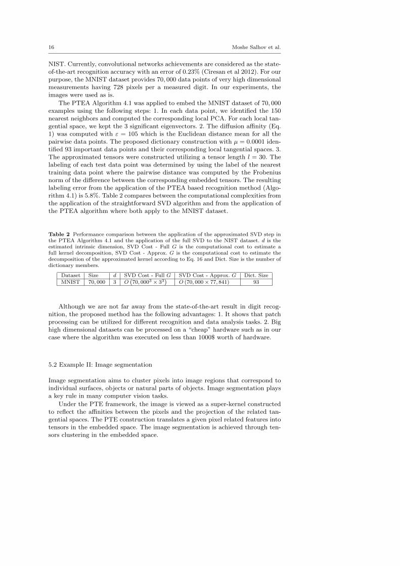
NIST. Currently, convolutional networks achievements are considered as the state-of-the-art recognition accuracy with an error of 0.23% (Ciresan et al 2012). For ourpurpose, the MNIST dataset provides 70, 000 data points of very high dimensionalmeasurements having 728 pixels per a measured digit. In our experiments, theimages were used as is.

The PTEA Algorithm 4.1 was applied to embed the MNIST dataset of 70, 000examples using the following steps: 1. In each data point, we identified the 150nearest neighbors and computed the corresponding local PCA. For each local tan-gential space, we kept the 3 significant eigenvectors. 2. The diffusion affinity (Eq.1) was computed with ε = 105 which is the Euclidean distance mean for all thepairwise data points. The proposed dictionary construction with µ = 0.0001 iden-tified 93 important data points and their corresponding local tangential spaces. 3.The approximated tensors were constructed utilizing a tensor length l = 30. Thelabeling of each test data point was determined by using the label of the nearesttraining data point where the pairwise distance was computed by the Frobeniusnorm of the difference between the corresponding embedded tensors. The resultinglabeling error from the application of the PTEA based recognition method (Algo-rithm 4.1) is 5.8%. Table 2 compares between the computational complexities fromthe application of the straightforward SVD algorithm and from the application ofthe PTEA algorithm where both apply to the MNIST dataset.

Table 2 Performance comparison between the application of the approximated SVD step inthe PTEA Algorithm 4.1 and the application of the full SVD to the NIST dataset. d is theestimated intrinsic dimension, SVD Cost - Full G is the computational cost to estimate afull kernel decomposition, SVD Cost - Approx. G is the computational cost to estimate thedecomposition of the approximated kernel according to Eq. 16 and Dict. Size is the number ofdictionary members.

Dataset Size d SVD Cost - Full G SVD Cost - Approx. G Dict. SizeMNIST 70, 000 3 O

(70, 0003 × 33

)O (70, 000× 77, 841) 93

Although we are not far away from the state-of-the-art result in digit recog-nition, the proposed method has the following advantages: 1. It shows that patchprocessing can be utilized for different recognition and data analysis tasks. 2. Bighigh dimensional datasets can be processed on a “cheap” hardware such as in ourcase where the algorithm was executed on less than 1000$ worth of hardware.

5.2 Example II: Image segmentation

Image segmentation aims to cluster pixels into image regions that correspond toindividual surfaces, objects or natural parts of objects. Image segmentation playsa key rule in many computer vision tasks.

Under the PTE framework, the image is viewed as a super-kernel constructedto reflect the affinities between the pixels and the projection of the related tan-gential spaces. The PTE construction translates a given pixel related features intotensors in the embedded space. The image segmentation is achieved through ten-sors clustering in the embedded space.


For the image segmentation examples, we utilized the pixel color informationand its spatial (x,y) location multiplied by a scaling factor w = 0.1. Hence, givena RGB image with Ix× Iy pixels, we generated the dataset X of size 5× (Ix · Iy).

Algorithm 4.1 is applied to construct an embedding of X into a tensor space.The first step in Algorithm 4.1 constructs local patches. Each generated patchcaptures the relevant neighborhood and considers both color and spatial similar-ities. Hence, a patch is more likely to include attributes related to spatially closepixels. It is important to note that the affinity kernel is computed according toEq. 1 where ε equals to the mean Euclidean distance between all pairs in X. ThePTE parameters l and ρ were chosen to generate homogeneous segments. The dic-tionary’s approximation tolerance µ was chosen arbitrarily to be µ = 0.001. Thek-means algorithm with sum of square differences clustered the tensors into similarclusters. The final clustering results from the embedded tensors as a function ofthe diffusion transition time t (Eq. 6) are presented in Figs. 2 and 3.

Figures 2 and 3 are the segmentated outputs from the application of the PTEAAlgorithm 4.1. In each figure, (a) is the original image. The images’ sizes are40 × 77 and 104 × 128, respectively. Each figure describes the output from thesegmentation as a function of the diffusion parameter t. The effect of the diffusiontransition time on the segmentation of the ‘Hand’ image is significant. For example,the first three images in Fig. 2, which correspond to t = 1, t = 2 and t = 3,respectively, show a poor segmentation results. As t increases, the segmentationbecomes more homogenous, thus the main structures in the original image can beseparated. For example, see t = 4 in (e). Another consequence from the increasein the diffusion transition time parameter t is the smoothing effect on the pairwisedistances between data points in the embedded space. By increasing t, the pairwisedistances between similar tensors are reduced while he distances between dissimilartensors increase.

(a) (b) (c) (d)

(e) (f) (g) (h)

Fig. 2 Segmentation results from the application of the PTEA Algorithm 4.1 to ‘Hand’ whenl = 10 and d = 10. (a) Original image. (b) Segmentation when t = 1. (c) Segmentation whent = 2. (d) Segmentation when t = 3. (e) Segmentation when t = 4. (f) Segmentation whent = 5. (g) Segmentation when t = 6. (h) Segmentation when t = 7.


(a) (b) (c) (d) (e) (f) (g) (h)

Fig. 3 Segmentation results from the application of the PTEA Algorithm 4.1 to ‘Sport’ withl = 10 and d = 20. (a) Original image. (b) Segmentation when t = 1. (c) Segmentation whent = 2. (d) Segmentation when t = 3. (e) Segmentation when t = 4. (f) Segmentation whent = 5. (g) Segmentation when t = 6. (h) Segmentation when t = 7.

Table 3 compares between the estimated computational complexity from theapplication of the approximated SVD by the PTEA Algorithm 4.1 and the com-putational complexity from the application of the full SVD by the PTE. Thegenerated dataset for each image consists of 13312 and 3080 data points, respec-tively. The computational complexity from the application of the approximatedSVD is significantly lower from the application of the full SVD in both cases.

Table 3 Performance comparison between the application of the approximated SVD stepin the PTEA Algorithm 4.1 and the application of the full SVD to the imaging datasets. dis the estimated intrinsic dimension, SVD Cost - Full G is the computational complexity toestimate a full kernel decomposition, SVD Cost - Approx. G is the computational complexityto estimate the decomposition of the approximated kernel according to Eq. 16 and Dict. Sizeis the number of dictionary members.

Image Size d SVD Cost - Full G SVD Cost - Approx. G Dict. SizeHand 104× 128 2 O

(266243

)O (26624× 16) 2

Sport 40× 77 2 O(61603

)O (6160× 16) 2

The constructed dictionary enables us to practically utilize the PTE for seg-menting medium sized images. The computational complexities were significantlyreduced in comparison to the application of the SVD decomposition that utilizesthe full super-kernel. The reduction in the computational complexity of image seg-mentation was achieved by the application of the dictionary-based SVD/QR stepof the extension coefficient matrix E in the PTEA algorithm.

5.3 Example III: Vector Field Extension over a Sphere

In this example, we utilize a synthetic vector field F . The synthetic vector fieldconsists of |M | = N = 8050 points sampled from a two dimensional half sphereM that is immersed in R3 by F : M → R3 such that for any x ∈ M , we haveF (x) ∈ Tx(M). For each two-dimensional data point, we generate a vector thatlies on the tangent plane of the sphere at a corresponding data point. Figure 4illustrates the described vector field from two views.


(a) (b)

Fig. 4 The generated vector field. (a) Full view. (b) Zoom.

The dictionary in this example is constructed using Algorithm 4.1 with themeta-parameters ε = 0.0218 and µ = 0.0005. The resulting dictionary containsηN = 414 members. Figure 5 presents the dictionary members that provide analmost uniform sampling of the sphere.

(a) (b)

Fig. 5 The generated vector field (arrows) and the chosen dictionary members (circles). (a)Full view. (a) Zoom.

Under the above settings, the vector OTx F (x) is a coordinate vector of F (x) inthe local basis of Tx(M). Our goal is to extend F to any data point y ∈ M\M .In our example, for each data point x ∈ M , we have a closed form for its lo-cal patch. Each patch at the data point x = (x1, x2) is spanned by two vectorsS1 = (1, 0,−x1

√1− x21 − x22) and S2 = (0, 1,−x2

√1− x21 − x22). Hence, the cor-

responding tangential space Ox is given by the application of SVD to [S1, S2]T .Furthermore, we choose the vectors from the vector field to be the correspondingvector F (x) = (1, 0,−x1

√1− x21 − x22). Equation 20 provides the solution to the

extension problem given the dictionary members and the corresponding super-kernel. For each data point y, which is not in the dictionary, we compute Eq. 5to find the extended vector field. The resulting vector field is compared with theoriginal vector field in Fig. 6.


(a) (b)

Fig. 6 The extended vector field (red) and the given vector field (blue). (a) Full view. (b)Zoom.

In order to evaluate the performance of this extension, we compared betweenthe length and the direction of the corresponding vector in the original vector field.Figure 7 displays the cumulative distribution function of these squared errors. Thecumulative distribution function in Fig. 7 suggests that, in comparison with theground truth vector field, about 93% of the estimated vectors have a vector lengthsquare error of less than 10−2, and 95% have vector direction square error of lessthan 2 · 10−2 radians.


(a)

(b)

Fig. 7 The cumulative distribution function of MSE of (a) Estimated vector length. (b)Estimated vector direction.

6 Conclusions

The proposed construction in the paper extends the dictionary construction in (En-gel et al 2004) by using the LPD super-kernel from (Salhov et al 2012; Wolf andAverbuch 2013). This is done by an efficient dictionary-based construction assum-ing the data is sampled from an underlying manifold while utilizing the non-scalarrelations and the similarities among manifold patches instead of representing themby individual data points. The constructed dictionary, which contains these patchesfrom the underlying manifold, are represented by the embedded tensors from (Sal-hov et al 2012), instead of representing them by individual data points. Therefore,it encompasses multidimensional similarities between local areas in the data. ThePTEA Algorithm reduces the computational complexities of the spectral analysisin comparison to the regular use of PTE based algorithm.


Acknowledgements

This research was supported by the Israel Science Foundation (Grant No. 1041/10),the Israel Ministry of Science & Technology (Grants No. 3-9096, 3-10898), by US- Israel Binational Science Foundation (BSF 2012282) and by a Fellowship fromUniversity of Jyvaskyla. The third author was supported by the Eshkol Fellowshipfrom the Israel Ministry of Science & Technology.

References

Ballester C, Bertalmio M, Sapiro G, Verdera J (2001) Filling-in by joint interpolation of vectorfields and gray levels. IEEE Trans Image Processing 10:1200–1211

Belkin M, Niyogi P (2003) Laplacian eigenmaps for dimensionality reduction and data repre-sentation. Neural Computation 15(6):1373–1396

Bermanis A, Averbuch A, Coifman R (2013) Multiscale data sampling and function extension.Applied and Computational Harmonic Analysis 34:182 – 203

Bomba JS (1959) Alpha-numeric character recognition using local operations. In: Paperspresented at the December 1-3, 1959, eastern joint IRE-AIEE-ACM computer confer-ence, ACM, New York, NY, USA, IRE-AIEE-ACM ’59 (Eastern), pp 218–224, DOI10.1145/1460299.1460325, URL http://doi.acm.org/10.1145/1460299.1460325

Bronstein M, Bronstein A (2011) Shape recognition with spectral distances. PatternAnalysis and Machine Intelligence, IEEE Transactions on 33(5):1065–1071, DOI10.1109/TPAMI.2010.210

Ciresan D, Meier U, Schmidhuber J (2012) Multi-column deep neural networks for image clas-sification. In: Computer Vision and Pattern Recognition (CVPR), 2012 IEEE Conferenceon, pp 3642–3649, DOI 10.1109/CVPR.2012.6248110

Coifman R, Lafon S (2006) Diffusion maps. Applied and Computational Harmonic Analysis21(1):5–30

Cox T, Cox M (1994) Multidimensional Scaling. Chapman and Hall, London, UKCullum JK, Willoughby RA (2002) Lanczos algorithms for large symmetric eigenvalue com-

putations. Society for Industrial ans Applied Mathematics 1David G (2009) Anomaly detection and classification via diffusion processes in hyper-networks.

PhD thesis, School of Computer Science, Tel Aviv UniversityDavid G, Averbuch A (2012) Hierarchical data organization, clustering and

denoising via localized diffusion folders. Applied and ComputationalHarmonic Analysis 33(1):1 – 23, DOI 10.1016/j.acha.2011.09.002, URLhttp://www.sciencedirect.com/science/article/pii/S1063520311000881

Dimond TL (1958) Devices for reading handwritten characters. In: Papers and discussionspresented at the December 9-13, 1957, eastern joint computer conference: Computers withdeadlines to meet, ACM, New York, NY, USA, IRE-ACM-AIEE ’57 (Eastern), pp 232–237,DOI 10.1145/1457720.1457765, URL http://doi.acm.org/10.1145/1457720.1457765

Engel Y, Mannor S, Meir R (2004) The kernel recursive least-squares algorithm. Signal Pro-cessing, IEEE Transactions on 52(8):2275 – 2285

Fowlkes C, Belongie S, Chung F, Malik J (2004) Spectral grouping using the nystrom method.IEEE TRANSACTIONS ON PATTERN ANALYSIS AND MACHINE INTELLIGENCE26

Fuselier EJ, Wright G (2009) Stability and error estimates for vector field interpolation anddecomposition on the sphere with rbfs. SIAM J Numer Anal 47(5):3213–3239, DOI10.1137/080730901, URL http://dx.doi.org/10.1137/080730901

Golub G, Van Loan C (2012) Matrix Computations, vol 4th Edition. John Hopkins UniversityPress

Jingen L, Yang Y, Shah M (2009) Learning semantic visual vocabularies using diffusion dis-tance. In: Computer Vision and Pattern Recognition, 2009. CVPR 2009. IEEE Conferenceon, pp 461–468, DOI 10.1109/CVPR.2009.5206845

Keller Y, Coifman R, Lafon S, Zucker S (2010) Audio-visual group recognition us-ing diffusion maps. Signal Processing, IEEE Transactions on 58(1):403–413, DOI10.1109/TSP.2009.2030861


Keysers D, Deselaers T, Gollan C, Ney H (2007) Deformation models for image recognition.IEEE Trans PAMI 29

Kruskal J (1964) Multidimensional scaling by optimizing goodness of fit to a nonmetric hy-pothesis. Psychometrika 29:1–27

Lafon S, Keller Y, Coifman R (2006) Data fusion and multicue data matching by diffusionmaps. Pattern Analysis and Machine Intelligence, IEEE Transactions on 28(11):1784–1797,DOI 10.1109/TPAMI.2006.223

Lecun Y, Bottou L, Bengio Y, Haffner P (1998) Gradient-based learning applied to documentrecognition. In: Proceedings of the IEEE, pp 2278–2324

Liu S, Trenkler G (2008) Hadamard, khatri-rao, kronecker and other matrix products. Inter-national Journal of Information & Systems Sciences 4(1):160–177

von Luxburg U (2007) A tutorial on spectral clustering. Statistics and Computing 17Rao CKC (1968) Solutions to some functional equations and their applications to character-

ization of probability distributions. Sankhya: The Indian Journal of Statistics, Series A(1961-2002) 30(2):pp. 167–180, URL http://www.jstor.org/stable/25049527

Rui X, Damelin S, Wunsch D (2007) Applications of diffusion maps in gene expression data-based cancer diagnosis analysis. In: Engineering in Medicine and Biology Society, 2007.EMBS 2007. 29th Annual International Conference of the IEEE, pp 4613–4616, DOI10.1109/IEMBS.2007.4353367

Salhov M, Wolf G, Averbuch A (2012) Patch-to-tensor embedding. Applied and ComputationalHarmonic Analysis 33(2):182 – 203, DOI 10.1016/j.acha.2011.11.003

Schclar A, Averbuch A, Rabin N, Zheludev V, Hochman K (2010) Adiffusion framework for detection of moving vehicles. Digital Sig-nal Processing 20(1):111 – 122, DOI 10.1016/j.dsp.2009.02.002, URLhttp://www.sciencedirect.com/science/article/pii/S1051200409000074

Singer A, Coifman R (2008) Non-linear independent component analysis with diffusion maps.Applied and Computational Harmonic Analysis 25(2):226–239

Singer A, Wu H (2011) Orientability and diffusion maps. Applied and Computational HarmonicAnalysis 31(1):44–58

Singer A, Wu H (2012) Vector diffusion maps and the connection laplacian. Communicationson Pure and Applied Mathematics 65(8):1067–1144

Suen C, Berthod M, Mori S (1980) Automatic recognition of handprinted characters ;the stateof the art. Proceedings of the IEEE 68(4):469 – 487, DOI 10.1109/PROC.1980.11675

Talmon R, Cohen I, Gannot S (2011) Supervised source localization using diffusion kernels.In: Applications of Signal Processing to Audio and Acoustics (WASPAA), 2011 IEEEWorkshop on, pp 245–248, DOI 10.1109/ASPAA.2011.6082267

Talmon R, Kushnir D, Coifman R, Cohen I, Gannot S (2012) Parametrization of linear systemsusing diffusion kernels. Signal Processing, IEEE Transactions on 60(3):1159–1173, DOI10.1109/TSP.2011.2177973

Talmon R, Cohen I, Gannot S (2013) Single-channel transient interference suppression withdiffusion maps. IEEE transactions on audio, speech, and language processing 21(1-2):132–144

Wolf G, Averbuch A (2013) Linear-projection diffusion on smooth Euclidean submanifolds.Applied and Computational Harmonic Analysis 34:1 – 14

learning from patches by e cient spectral decomposition of

Documents