learning algorithm and application of quantum neural ... · abstract—a novel neural networks...
TRANSCRIPT

Abstract—A novel neural networks model with quantum
weights is present. Firstly, based on the information processing
modes of biology neuron and quantum computing theory, a
quantum neuron model is presented, which is composed of
weighting, aggregating, activating, and inspiriting. Secondly the
quantum neural networks model based on quantum neuron is
constructed in which the input and the output are real vectors;
the linked weight and the activation value are qubits. On the
basic of the gradient descent algorithm, a learning algorithm of
this model is proposed. It is shown that this algorithm is
super-linearly convergent under certain conditions and can
increase the probability of getting the global optimal solution.
Finally, the availability of the model is illustrated in both
convergence speed and convergence rate by two application
examples of pattern recognition and function approximation.
Index Terms—Quantum computing, quantum neuron,
quantum neural network, super-linear convergence
I. INTRODUCTION
Artificial Neural Network (ANN) has widely been applied
to every field since M-P model of neuron is proposed. ANN
has gained the great development through decades of
research, at the same time some problems is also appeared.
Because it is based on the simplistic neuron model, ANN
cannot satisfy the increasing demands of quantity and
complexity of information. Therefore, it is one of the farther
directions of development and research for the ANN to
construct the perfect ANN theory and to endure with the
more comprehensive mathematics basis, biology feature, and
physical feature [1].
The combination of quantum computation and neural
networks is a rising subject of ANN theory research, and the
research of Quantum Neural Networks (QNN) has just begun.
At present, many QNN research results have been acquired in
international since the comparability comment on quantum
theory and neural network theory is proposed by Perus.
Menneer and Narayanan proposed a method in which
introduce the multi-universe theory in quantum mechanics
into neural network training, exists a neural network
corresponding each sample in training set, and total networks
is made up of superposition of these networks. Behrman et al.
Manuscript received November 24, 2012; revised January 25, 2013. This
work was supported in part by the Information Center of Daqing Oilfield
Company. Ltd.
D. B. Mu is with the visit scholar with University of Waterloo, Canada
(e-mail: [email protected]).
Z. Y. Guan is with the Information Center of Daqing Oilfield, China
(e-mail: [email protected]).
H. Zhang is with the Oil and gas well production data management system
(A2) of Daqing Oilfield Company. China (e-mail:
proposed a QNN model realized by an array of quantum dot
molecules. In this model, a single quantum dot molecule is
adopted for every input, the system is evolved in real time
according to quantum mechanics, measures is performed by
fixed time interval, and the different time pieces are regarded
as the neurons in hidden layer. Therefore, the more time
pieces the measures applies, the more hidden neurons the
model has. As present, the QNN research direction
approximately includes: the quantum associative memory [2],
[3], the quantum competition learning [4], the neural network
applied quantum dots [5], the common neural network
applied quantum transform function, and the quantum
Hopfield networks and so on. Ref. [6] proposed neural
networks with quantum gated nodes and indicated that such
quantum networks may contain some advantageous features
of biological systems more efficiently than classical
electronic devices in 2007. Ref. [7] has proposed a quantum
BP neural networks model with learning algorithm based on
single-qubit rotation gate and two-qubit controlled-NOT
gates.
The research presented in this paper (a) constructs
quantum neuron and quantum neural network model based
on the feature of biology neuron and quantum mechanics, in
which the linked weight and the activation value is expressed
in qubits, (b) proposes an learning algorithm for this model,
and prove this algorithm is super- linearly convergent under
certain conditions, and can increase the convergence
probability, (c) designs two experiments, the results show
that this model and algorithm are superior to the common BP
(CBP) neural network in both the convergence speed and the
convergence rate.
II. QUANTUM NEURAL NETWORK MODEL
A. Quantum Neuron Model
The biology research shows that, in biology neuron, the
nerve impulse introduced from other neurons can induce the
change of voltage differences between the voltage inside cell
velum and that outside cell velum. This change can associate
with the current activation value and can update it. When the
activation value is greater than a certain threshold value, the
neuron activation is inspired, the voltage inside cell velum
sharp rises, and the electricity pulse (nerve impulse) is
released by the neuraxon [7], [8]. Therefore, the information
disposal process of the biology neuron includes four parts:
weighting, aggregating, activating, and inspiriting. Some
research results in the 1990s shows that the information
disposal process of brain might be concerned with quantum
phenomenon, the quantum mechanics effect, and the
Learning Algorithm and Application of Quantum Neural
Networks with Quantum Weights
Dianbao Mu, Zunyou Guan, and Hong Zhang
International Journal of Computer Theory and Engineering, Vol. 5, No. 5, October 2013
788DOI: 10.7763/IJCTE.2013.V5.797
quantum system has the similar dynamics feature to the
biology neural networks [9]. Therefore, the combination of
ANN and quantum theory might perfectly simulate the
information disposal process of brain.
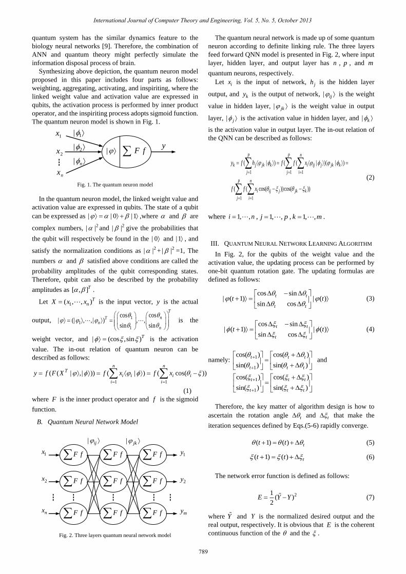
Synthesizing above depiction, the quantum neuron model
proposed in this paper includes four parts as follows:
weighting, aggregating, activating, and inspiriting, where the
linked weight value and activation value are expressed in
qubits, the activation process is performed by inner product
operator, and the inspiriting process adopts sigmoid function.
The quantum neuron model is shown in Fig. 1.
Fig. 1. The quantum neuron model
In the quantum neuron model, the linked weight value and
activation value are expressed in qubits. The state of a qubit
can be expressed as | | 0 |1 ,where and are
complex numbers, 2| | and 2| | give the probabilities that
the qubit will respectively be found in the | 0 and | 1 , and
satisfy the normalization conditions as 2| | + 2| | =1, The
numbers and satisfied above conditions are called the
probability amplitudes of the qubit corresponding states.
Therefore, qubit can also be described by the probability
amplitudes as [ , ]T .
Let 1( , , )TnX x x is the input vector, y is the actual
output, 1
11
coscos| (| , ,| ) , ,
sin sin
T
nTn
n
is the
weight vector, and | (cos ,sin )T is the activation
value. The in-out relation of quantum neuron can be
described as follows:
1 1
( ( | ,| )) ( | ) ( cos( ))
n nT
i i i i
i i
y f F X f x f x
(1)
where F is the inner product operator and f is the sigmoid
function.
B. Quantum Neural Network Model
Fig. 2. Three layers quantum neural network model
The quantum neural network is made up of some quantum
neuron according to definite linking rule. The three layers
feed forward QNN model is presented in Fig. 2, where input
layer, hidden layer, and output layer has n , p , and m
quantum neurons, respectively.
Let ix is the input of network, jh is the hidden layer
output, and ky is the output of network, | ij is the weight
value in hidden layer, | jk is the weight value in output
layer, | j is the activation value in hidden layer, and | k
is the activation value in output layer. The in-out relation of
the QNN can be described as follows:
1 1 1
1 1
( | ) ( ( | ) | )
( ( cos( ))cos( ))
p p n
k j jk k i ij j jk k
j j i
p n
i ij j jk k
j i
y f h f f x
f f x
(2)
where 1, ,i n , 1, ,j p , 1, ,k m .
III. QUANTUM NEURAL NETWORK LEARNING ALGORITHM
In Fig. 2, for the qubits of the weight value and the
activation value, the updating process can be performed by
one-bit quantum rotation gate. The updating formulas are
defined as follows:
cos sin| ( 1) | ( )
sin cos
t t
t t
t t
(3)
cos sin| ( 1) | ( )
sin cos
t t
t t
t t
(4)
namely: 1
1
cos( ) cos( )
sin( ) sin( )
t t t
t t t
and
1
1
cos( ) cos( )
sin( ) sin( )
t t t
t t t
Therefore, the key matter of algorithm design is how to
ascertain the rotation angle t and t that make the
iteration sequences defined by Eqs.(5-6) rapidly converge.
( 1) ( ) tt t (5)
( 1) ( ) tt t (6)
The network error function is defined as follows:
21( )
2E Y Y (7)
where Y and Y is the normalized desired output and the
real output, respectively. It is obvious that E is the coherent
continuous function of the and the .
F f
F f
F f
F f
F f
F f
F f
F f
F f
1x
2x
┇
nx
┇ ┇ ┇ ┇
1y
2y
my
| ij
| jk
fF
1x
2x
nx
1|
2|
n|
y
┇
|
International Journal of Computer Theory and Engineering, Vol. 5, No. 5, October 2013
789

Lemma. Suppose ( ) *t ,
let ( ) ( ) *t t , ( ) ( 1) ( ) ( 1) ( )t t t t t .
Then that the sequence ( )t is super-linearly convergent is
equal to ( 1) ( )t o t [10].
There exists the following theorem about the computation
of rotation angle and of quantum gate.
Theorem 1. When and is respectively computed
according to Eq.(8) and Eq.(9) and 2r , the iteration
sequences )(t and )(t are super-linearly convergent.
1( ( ), ( ))
( ) ( )( ( ( ), ( )))( )
rE t t
t E t tt
(8)
1( ( ), ( ))
( ) ( )( ( ( ), ( )))( )
rE t t
t E t tt
(9)
where is the learning rate.
Proof. Firstly, prove the convergence of two sequences.
According to Thaler formula
( ( 1), ( 1)) ( ( ), ( ))E t t E t t
( ( ), ( ))
( ) ( )( )
( ) ( ( ), ( )) ( )
( )
T T
E t t
t ttO
t E t t t
t
2 2 1( ( ), ( )) ( ( ), ( ))
( ( ( ), ( )))( ) ( )
rE t t E t t
E t tt t
Therefore ( ( 1), ( 1)) ( ( ), ( )) 0E t t E t t , namely,
the iteration sequences ( )t and ( )t is monotone
reductive. On the other hand, ( ( ), ( ))E t t has the lower
boundary, therefore, there certainly exists the limit of
sequence. Because ( ( ), ( ))E t t is the coherent continuous
function of and , therefore, exist equation as follows:
lim( ( ), ( )) ( *, *)t
t t
, namely, the iteration sequences
( )t and ( )t are convergent.
Secondly, applying the method of Ref. [10], prove the
super- linearity of the sequence convergence.
Let
max
( ( ), ( ))
( )
E t tA
t
, then
1
( 1) ( 1) *
( ) ( ( ), ( ))( )( ( ( ), ( )))
( )r
t t
t E t tE t t
t
1
( 1) *
( ( ( ), ( ))) r
t
A E t t
Because ( ( ), ( ))E t t is the quadratic equation of
( )t and ( )t , when 2r , ( 1) *t
1
( ( ( ), ( ))) rO E t t
. Therefore ( 1) ( )t O t .
According to the lemma, the iteration sequence ( )t is
super-linearly convergent. With the same reasoning, the
iteration sequence ( )t is also super-linearly convergent.
Theorem 2. If * and * is the convergent solutions of
sequence ( )t and ( )t , respectively, then any * and
* defined by * * * * is also the convergent
solutions of sequence ( )t and ( )t , respectively.
Proof. Because * and * is the convergent solution of
sequence ( )t and ( )t , respectively, according to
Eq.(2), the network output is described as follows:
* * * *
1 1
( ( cos( ))cos( ))
p n
k i ij j jk k
j i
y f f x
* * * *
1 1
( ( cos( ( )))cos( ( )))
p n
i ij j jk k
j i
f f x
* * * *
1 1
( ( cos( ))cos( ))
p n
i ij j jk k k
j i
f f x y
Therefore * and * is also the convergent solutions of
sequence ( )t and ( )t , respectively. Where ky is
desired output corresponding ky .
Theorem 1 assures the speediness of network convergence.
Theorem 2 assures the diversity of convergent solutions,
which only demands the phase difference between | and
| satisfy a certain condition, and ignore the actual phase
values of | and | . Therefore, this algorithm can
evidently increase the convergence probability.
Synthesizing above depiction, the algorithm proposed in
this paper is described as follows: Step1: Initialize the network parameters. Including: the
node number of each layer, restriction error , the maximum
of iterative steps Max , set the current iterative step 0t .
Step2: Initialize the weights value and the activation
values. Hidden layer:
(0) 2 Rndij ; (0) 2 Rndj ;cos( (0))
sin( (0))
ij
ijij
;
cos( (0))
sin( (0))
j
jj
Output layer:
(0) 2 Rndjk ; (0) 2 Rndk ;cos( (0))
sin( (0))
jk
jkjk
;
cos( (0))
sin( (0))
kk
k
where 1, ,i n , 1, ,j p , 1, ,k m , Rnd is a random
number in [0,1].
International Journal of Computer Theory and Engineering, Vol. 5, No. 5, October 2013
790
Step3: Compute network output according to Eq.(2), and
update the weight value and activation value of each layer
according to Eqs.(3-4).
Step4: Compute the output error according to Eq.(7), if
E or Maxt , then go to step5,else 1 tt , go back
Step3.
Step5: Save the weight values and activation values of
each layer.
IV. COMPARISON EXPERIMENT
In the classical computer, the information disposal process
is performed by logic gate. The quantum states in quantum
register evolve through the quantum gate. In Hilbert space, as
its linear restriction, the quantum gate would simultaneously
have an effect on all quantum ground states, which is equal to
computing 2n numbers at one time, however, any classical
computer need to repeat 2n computations or need to 2n
parallel processor to the same task. This is the parallel
quantum computation. In the other words, the entanglement
and the superposition of quantum information in the quantum
computer presents the great advantage, which is proved by
Shor algorithm. However, the hardware realization of
quantum circuit and quantum algorithm has been proved to
be an austere challenge, especially, the applied quantum
computers are being researching [11].
Therefore, the algorithm proposed in this paper cannot be
realized in computer equipped with the quantum hardware,
and cannot test the great advantage brought by the parallel
quantum computation. But the quantum theory makes the
QNN differ from the common neural network in information
process mode. In QNN, the weight value qubits are rotated in
a unit circle by the quantum rotation gate. According to
theorem 1, these qubits can soon be matched to the optimum
place by setting the proper quantum gates rotation angle.
According to theorem 2, the number of the optimum
solutions in the QNN is far more than that in the common
neural network, and can evidently increase the convergence
probability, which can be tested in the common computer.
To testify the validity of QNN, two kinds of experiments
are designed and the QNN is compared with the common BP
network (CBP) in this part. To make comparison equitable,
the QNN adopts the same structure and parameters as CBP in
the experiments.
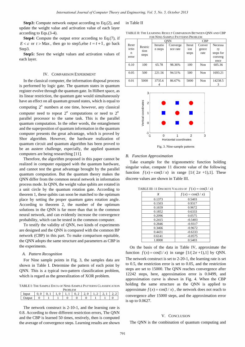
A. Pattern Recognition
For Nine sample points in Fig. 3, the samples data are
shown in Table I. Determine the pattern of each point by
QNN. This is a typical two-pattern classification problem,
which is regard as the generalization of XOR problem.
TABLE I: THE SAMPLE DATA OF NINE-SAMPLE PATTERNS CLASSIFICATION
PROBLEM
Input 0, 0 0, 1 1, 0 1, 1 0, 2 2, 0 1, 2 2, 1 2, 2
Output 0 1 1 0 0 0 1 1 0
The network construct is 2-10-1, and the learning rate is
0.8. According to three different restriction errors, The QNN
and the CBP is learned 50 times, restively, then is computed
the average of convergence steps. Learning results are shown
in Table II
TABLE II: THE LEARNING RESULT COMPARISON BETWEEN QNN AND CBP
FOR NINE-SAMPLE PATTERNS PROBLEM
Restr
ictio
n
error
Restric
tion
steps
QNN CBP
Iteratio
n steps
Converge
nce rate
Iterat
ion
steps
Conver
gence
rate
Necessa
ry
steps for
converg
ence
0.10 100 65.78 98.36% 100 Non
605.36
0.05 500 221.56 94.51% 500 Non
1693.21
0.01 5000 3735.6
4
86.67% 5000 Non
14238.5
3
-1 0 1 2 3-1
0
1
2
3
Horizontal coordinatesV
ert
ica
l co
ord
ina
tes
Fig. 3. Nine-sample patterns
B. Function Approximation
Take example for the trigonometric function holding
singular value, compute 11 discrete value of the following
function ( ) cos(1/ )f x x in range [1/( 2 +1),1]. These
discrete values are shown in Table III.
TABLE III: 11 DISCRETE VALUES OF ( ) cos(1 / )f x x
x ( ) cos(1 / )f x x
0.1373 0.5403
0.1503 0.9317
0.1659 0.9672
0.1852 0.6333
0.2096 0.0575
0.2415 -0.5403
0.2846 -0.9317
0.3466 -0.9672
0.4431 -0.6333
0.6141 -0.0575
1.0000 0.5403
On the basis of the data in Table IV, approximate the
function ( ) cos(1/ )f x x in range [1/( 2 +1),1] by QNN.
The network construct is set to 2-20-1, the learning rate is set
to 0.5, the restriction error is set to 0.05, and the restriction
steps are set to 15000. The QNN reaches convergence after
12242 steps, here, approximation error is 0.0499, and
approximation curve is shown in Fig. 4. When the CBP
holding the same structure as the QNN is applied to
approximate ( ) cos(1/ )f x x , the network does not reach to
convergence after 15000 steps, and the approximation error
is up to 0.0627.
V. CONCLUSION
The QNN is the combination of quantum computing and
International Journal of Computer Theory and Engineering, Vol. 5, No. 5, October 2013
791

nerve computing, which has the advantage such as
parallelism and high efficiency of quantum computation
besides continuity, approximation capability, and
computation capability that the general ANN has. In QNN,
the weight value and the activation value are expressed by
qubits, and the phase of each qubit is updated by the quantum
rotation gate. Since both probability amplitudes participate in
optimizing computation, the computation capability is
evidently superior to the general BP network. Experiment
proves that the QNN model and algorithm proposed in this
paper is effective.
0.1 0.3 0.5 0.7 0.9 1
-1
-0.5
0
0.5
1
Real curve
Approaching curve
Fig. 4. Function approximation curve
REFERENCES
[1] J. L. Cheng, D. H. Feng, and F. Liu, Immune Optimization
Computation, Learn and Recognition, Science Press, Beijing, 2006.
[2] D. Ventura and T. R. Martinez, “Quantum associative memory,”
Information Sciences, vol. 124, pp. 273-296, 2000.
[3] M. Perus and P. Ecimovic, “Memory and pattern recognition in
associative neural networks,” International Journal of Applied Science
and Computation, vol. 4, pp. 283-310, 1998.
[4] P. Pyllkkanen and P. Pylkko, “New directions in cognitive science,” in
Proc. the International Symposium. Saariselka, pp. 77-89, 1995.
[5] E. Behrman, “A quantum dot neural networks,” in Proc. Workshop
Physics of Computation. Cambridge, pp. 22-24, 1996.
[6] F. Shafee, “Neural networks with quantum gated nodes,” Engineering
Applications of Artificial Intelligence, vol. 20, no. 4, pp. 429-437,
2007.
[7] C. P. Li and S. Y. Li, “Learning algorithm and application of quantum
BP neural networks based on universal quantum gates,” Journal of
Systems Engineering and Electronics, vol. 19, no. 1, pp. 167-174,
2008.
[8] S. Y. Li, Fuzzy Control, Neurocontrol and Intelligent Cybernetics,
Harbin Institute of Technology Press, Harbin, 1998.
[9] M. Perus, “Neuro-quantum parallelism in brain-mind and computers,”
Informatics, vol. 20, pp. 173-183, 1996.
[10] L. J. Zhen, X. G. He, and D. S. Huang, “Super-linearly convergent bp
learning algorithm for feed forward neural networks,” Journal of
Software, in Chinese, vol. 11, no. 8, pp. 1094-1096, 2000.
Zunyou Guan was born on January 21, 1966 in
Songyuan City, Jilin Province, China, got bachelor's
degree in Daqing Petroleum Institute in 1988, majored
in Drilling Engineering, got master's degree in Jilin
University in 2007, majored in Software Engineering.
He started to work in information center of No1
Drilling Company of the Daqing Petroleum
Administration Bureau from 1991 to 1995, since 1995,
worked in the Information Center of Daqing Oilfield
Co., Ltd., a senior engineer, deputy director. He has made great achievements
and published numerous papers during these years. “The Digital
Development Framework and Implementation Strategy of Daqing Oilfield”
was published in “The Digital Chemical” in 2004; in 2005, “A Scalable Data
Quality Element Model” was published in “Computer Engineering”, "A
Large-scale Information Systems Project Implementation and Management
Practice on Information Systems Engineering " published in 2012, organized
by the Information Center of Tianjin.
International Journal of Computer Theory and Engineering, Vol. 5, No. 5, October 2013
792
[11] P. Knight, “Quantum information processing without entanglement,”
Science, vol. 287, pp. 441-442, 2000.
Dianbao Mu was born on March 9th 1975 in Harbin
Heilongjiang Province, China, graduated from the
Daqing Petroleum Institute in 2000 years, majored in
Computer Software. In 2004 start to learn in Jilin
University in Jilin province, China and got master
degree in 2007 majored in computational
Mathematics. In 2012, he went to University of
Waterloo Canada as a visit scholar. He started to work
as a computer engineer in the No.1 Oil Production
Company, in 2004, he moved to the Information Center of Daqing Oilfield
Company. Ltd. In 2010, he started to work as a senior engineer and started
the research of Quantum theory, and put emphases on the application in
Oilfield. During these years, he finished more than 10 projects As technique
expert, “Design of Takagi-Sugeno Fuzzy Controller Based on Improved
Quantum Genetic Algorithm” was published in Computer Engineering in
2011.
Hong Zhang was born on October 27, 1975 in Daqing
Heilongjiang Province, China. Graduated from the
Shenyang Industrial College in 1995, majored in
Machinery manufacturing. He started to work as a
computer engineer in the No.1 Oil Production
Company in 2000.in 2011, he moved to the Daqing
oilfield exploration and Development Institute. During
these years, he finished more than 4 projects as
technology expert, and has published many articles.
Now, he is in charge of the Oil and gas well production data management
system (A2) of Daqing Oilfield Company.