learning about the world part ii - petra...
TRANSCRIPT

Introduction to Statistics : Learning About The World
Introduction to StatisticsLearning About The World
Part II
Instructor : Siana Halim
-S. Halim -
Introduction to Statistics : Learning About The World
-S. Halim -
TOPICS
• Inferences About Means• Comparing Means• Paired Samples and Blocks• Comparing Counts
References:•De Veaux, Velleman , Bock, Stats, Data and Models, Pearson Addison WesleyInternational Edition, 2005•John A Rice, Mathematical Statistics and Data Analysis, Duxbury Press, 1995
Introduction to Statistics : Learning About The World
-S. Halim -
Introduction to Statistics : Learning About The World
-S. Halim -
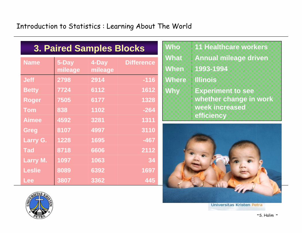
3. Paired Samples Blocks
Experiment to see whether change in work week increased efficiency
WhyIllinoisWhere1993-1994WhenAnnual mileage drivenWhat11 Healthcare workersWho
33626392106366061695499732811102617761122914
4-Day mileage
4451697
342112-46731101311-26413281612-116
Difference
3807Lee8089Leslie1097Larry M.8718Tad1228Larry G.8107Greg4592Aimee838Tom7505Roger7724Betty2798Jeff
5-Day mileage
Name

Introduction to Statistics : Learning About The World
-S. Halim -
Boxplots of the mileage don‘t show much. We can‘t tell whether the 4-day work week was succesful in reducing miles driven.
A two-sample t-test wouldn‘t help much either. (It would find a P-value of 0.4. clearly not evidence of a difference.) BUT wait a minute. The two-sample t-test is not valid here. We have 11 individuals, and we know their mileage before and after the change in schedule. These data are not independent.
Dat
a
C2C1
9000
8000
7000
6000
5000
4000
3000
2000
1000
0

Introduction to Statistics : Learning About The World
-S. Halim -
Paired Data
• Data such as these are called paired. Here, the independence assumption is violated, but we can actually do much better then the two-sample t-test.
• Paired data arise in a number of ways.The most common is to compare subjects with themselves before and after a treatment.
When pairs arise from an experiment, the pairing is a type of blocking.When pairs arise from an observational study, it is a form of matching.
Paired of spouses or siblings.Time series data

Introduction to Statistics : Learning About The World
-S. Halim -
• If you know the data are paired, you may not use the two-sample and pooled methods of the previous chapter.
• You must decide whether the data are paired from understanding how they were collected and what they mean (check the W‘s).
• There is no test to determine whether the data are paired.
Once we recognize that the mileage data are matched pairs, it makes sense to consider the change in annual miles driven for each worker as the work schedule changed. So we look at the collection of pairwise differences.

Introduction to Statistics : Learning About The World
-S. Halim -
Paired Data Assumption
Nearly normal condition can be checked with a histogram or Normal probability plot of differences.
Normal Population Assumption
Randomness can arise in one of two-ways:(1) The individuals may be a random sample.(2) In an experiment, the order of two treatments may be
randomly assigned, or the treatments may be randomly assigned to one member of each pair.
(3) In a before and after study, we may believe that the observed differences are a representative sample from a population of interest.
Randomization condition
If the data are paired, the groups are not independence. For this methods, it‘s the difference that must be independent of each other.
Independence Assumption
Introduction to Statistics : Learning About The World
-S. Halim -
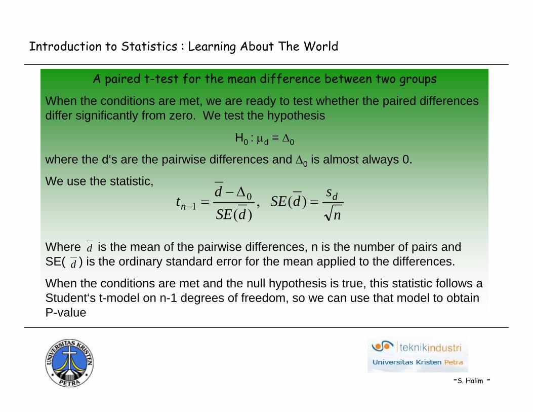
A paired t-test for the mean difference between two groups
When the conditions are met, we are ready to test whether the paired differences differ significantly from zero. We test the hypothesis
H0 : μd = Δ0
where the d‘s are the pairwise differences and Δ0 is almost always 0.
We use the statistic,
Where is the mean of the pairwise differences, n is the number of pairs and SE( ) is the ordinary standard error for the mean applied to the differences.
When the conditions are met and the null hypothesis is true, this statistic follows a Student‘s t-model on n-1 degrees of freedom, so we can use that model to obtain P-value
ns
dSEdSE
dt dn =
Δ−=− )(,
)(0
1
dd
Introduction to Statistics : Learning About The World
-S. Halim -
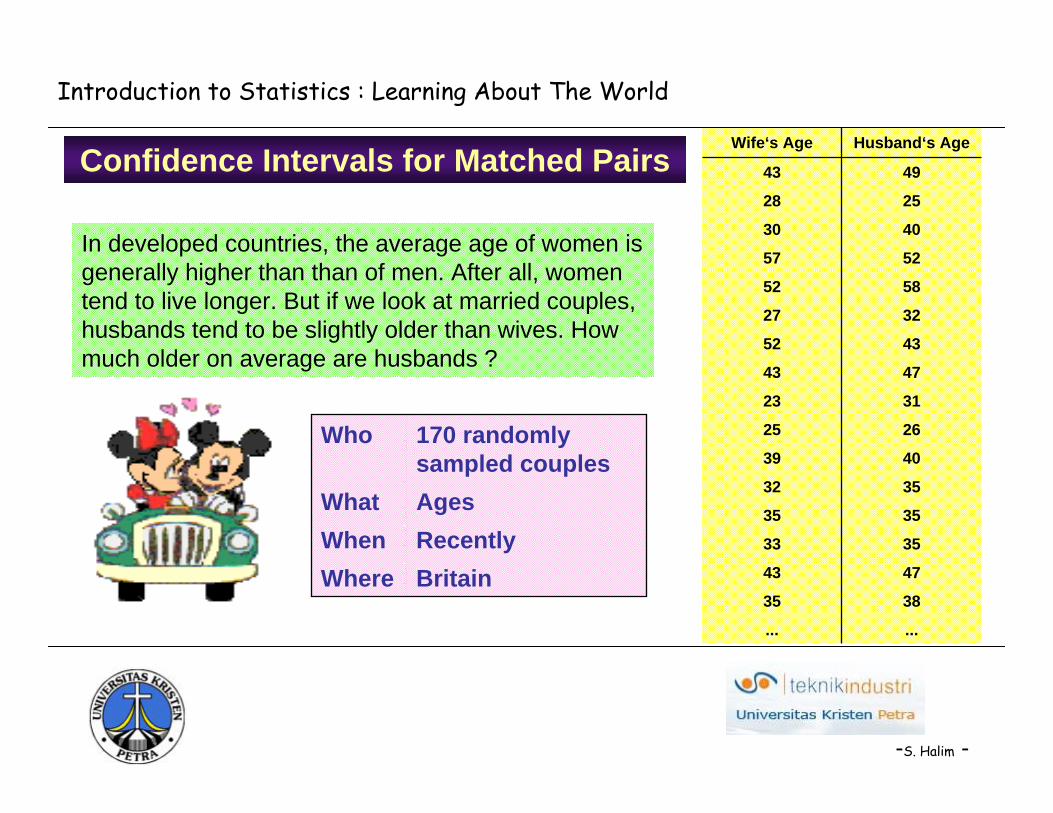
Confidence Intervals for Matched Pairs
BritainWhereRecentlyWhenAgesWhat
170 randomly sampled couples
Who
......
3835
4743
3533
3535
3532
4039
2625
3123
4743
4352
3227
5852
5257
4030
2528
4943
Husband‘s AgeWife‘s Age
In developed countries, the average age of women is generally higher than than of men. After all, women tend to live longer. But if we look at married couples, husbands tend to be slightly older than wives. How much older on average are husbands ?

Introduction to Statistics : Learning About The World
-S. Halim -
A paired t-interval
When the conditions are met, we are ready to find the confidence interval for the mean of the paired differences. The confidence interval is
The critical value t* depends on the particular confidence level, α, that you specify and on the degrees of freedom n-1, which is based on the number of pairs, n.
ns
dSEdSEtd dn =± − )(),(*
1

Introduction to Statistics : Learning About The World
-S. Halim -
Dat
a
HusbandWife
60
50
40
30
20
Blocking• Because the sample includes both older
and younger couples, there‘s a lot of variation in the ages of the men and in the ages of the women.
• In fact, that variation is so great that a boxplot of the two groups would show no difference. But that would be the wrong plot.
• It‘s the differences we care about.• Pairing removes the extra variation and
allows us to focus on the individual differences.
• In experiments, we block to separate the variability between the experimental units from the variability in the response.
Introduction to Statistics : Learning About The World
-S. Halim -
What Can Go Wrong ?
• Don‘t use a two-sample t-test for paired data• Don‘t use a paired t method when the samples aren‘t paired. When
two groups don‘t have the same number of valuee, it‘s pretty easy to see that they can‘t be paired. But just because two groups have the same number of observations doesn‘t mean they can be paired even if they are shown side-by-side in a table.
• Don‘t forget outliers in the differences. Be sure to plot the differences.
• Don‘t look for the difference in side-by-side boxplots. The point of the paired analysis is to remove extra variation. The boxplots of each group still contain the variation. Comparing them is likely to be misleading. A scatterplot of the two variables can sometimes be helpful.
Introduction to Statistics : Learning About The World
-S. Halim -
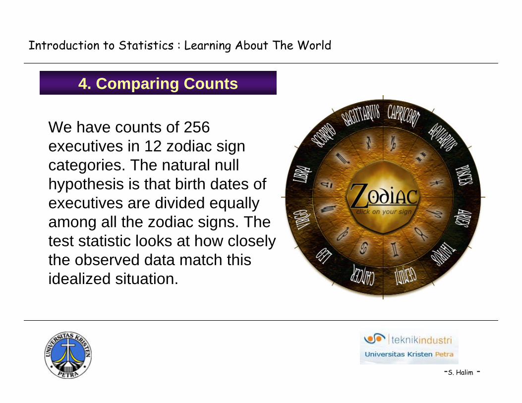
4. Comparing Counts
We have counts of 256 executives in 12 zodiac sign categories. The natural null hypothesis is that birth dates of executives are divided equally among all the zodiac signs. The test statistic looks at how closely the observed data match this idealized situation.

Introduction to Statistics : Learning About The World
-S. Halim -
A Chi-Square Test for Goodness-of-Fit
Pisces29Aquarius24Capricorn22Sagitarius19Scorpio21Libra18Virgo19Leo20Cancer23Gemini18Taurus20Aries23SignBirths
We want to know whether births of successful people are uniformly distributed across the signs of the zodiac.H0: Births are uniformly distributed over zodiac signs.H1: Births are not uniformly distributed over zodiac signs.
Hypotheses. State what we want to know
Introduction to Statistics : Learning About The World
-S. Halim -
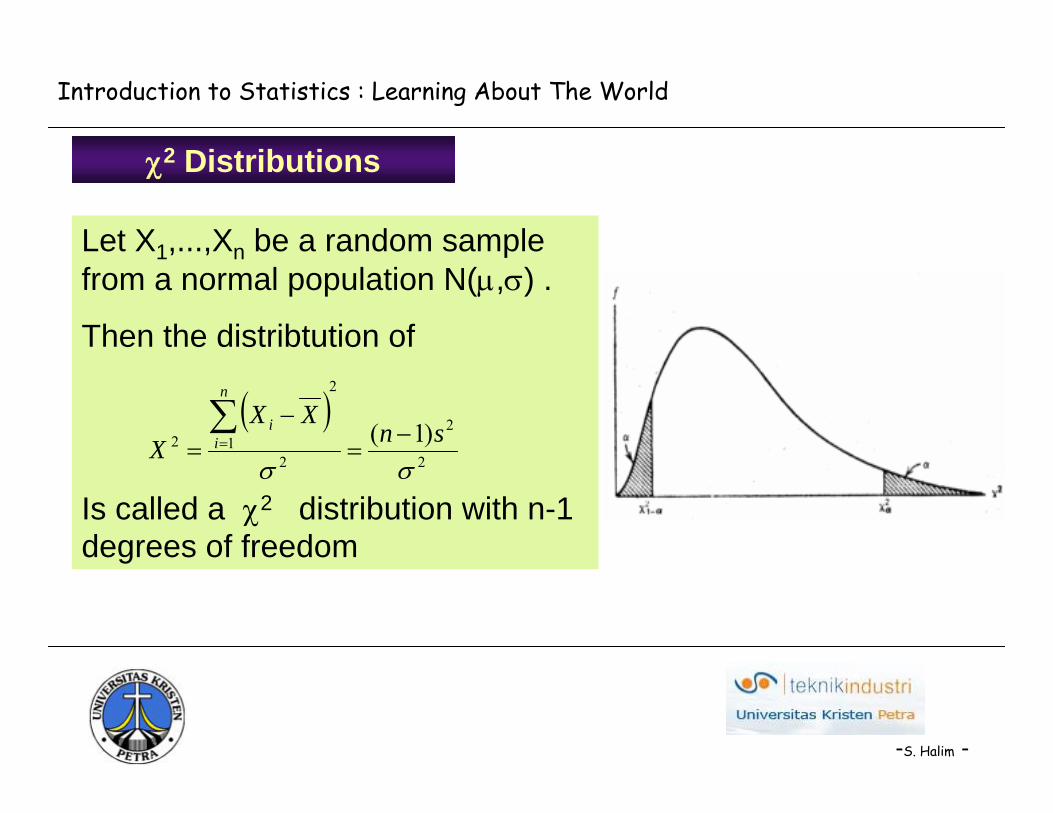
Let X1,...,Xn be a random sample from a normal population N(μ,σ) .
Then the distribtution of
Is called a χ2 distribution with n-1 degrees of freedom
( )2
2
2
2
12 )1(σσ
snXX
X
n
ii −
=−
=∑=
χ2 Distributions
-S. Halim -
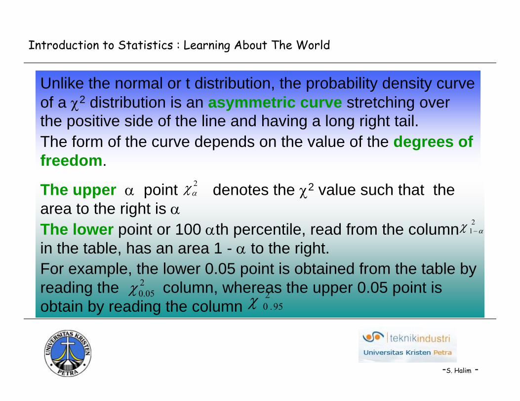
Unlike the normal or t distribution, the probability density curve of a χ2 distribution is an asymmetric curve stretching over the positive side of the line and having a long right tail. The form of the curve depends on the value of the degrees of freedom.
The upper α point denotes the χ2 value such that the area to the right is αThe lower point or 100 αth percentile, read from the column in the table, has an area 1 - α to the right.For example, the lower 0.05 point is obtained from the table by reading the column, whereas the upper 0.05 point is obtain by reading the column
2αχ
21 αχ −
295.0χ
205.0χ
Introduction to Statistics : Learning About The World
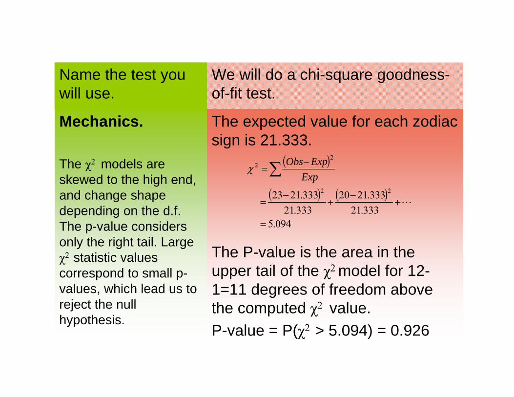
The expected value for each zodiac sign is 21.333.
The P-value is the area in the upper tail of the χ2 model for 12-1=11 degrees of freedom above the computed χ2 value.P-value = P(χ2 > 5.094) = 0.926
Mechanics.
The χ2 models are skewed to the high end, and change shape depending on the d.f. The p-value considers only the right tail. Large χ2 statistic values correspond to small p-values, which lead us to reject the null hypothesis.
We will do a chi-square goodness-of-fit test.
Name the test you will use.
( )
( ) ( )
094.5333.21
333.2120333.21
333.2123 22
22
=
+−
+−
=
−=∑
L
ExpExpObs
χ

Introduction to Statistics : Learning About The World
-S. Halim -
The p-value of 0.926 says that if the zodiac signs of executives were in fact distributed uniformly, an observed chi-square value of 5.09 or higher would occur about 93% of the time. We conclude that these data show virtually no evidence of non-uniform distribution of zodiac signs among executives.
Conclusion

Introduction to Statistics : Learning About The World
-S. Halim -
Comparing Observed Distributions
Many high schools survey graduation classes to determine the plans of the graduates. We might wonder whether the plans of students have stayed roughly the same over past decades or whether they have changed. Here is a summary table from one high school. Each cell of the table shows how many students from a particular graduating class (the column) made a certain choice (the row).
1058315290453Total245217Travel4251918Military139172498Employment
853288245320College/Post-HS education
Total200019901980

Introduction to Statistics : Learning About The World
-S. Halim -
100100100100Total2.271.590.693.75Travel3.971.596.553.97Military
13.145.408.2821.6Employment
80.6291.484.570.6College/Post-HS education
Total200019901980
Because the class sizes change so much, we’re probably better off examining the proportions for each class rather than the counts:
Introduction to Statistics : Learning About The World
-S. Halim -
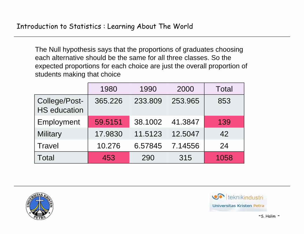
1058315290453Total247.145566.5784510.276Travel4212.504711.512317.9830Military
13941.384738.100259.5151Employment
853253.965233.809365.226College/Post-HS education
Total200019901980
The Null hypothesis says that the proportions of graduates choosing each alternative should be the same for all three classes. So the expected proportions for each choice are just the overall proportion of students making that choice

Introduction to Statistics : Learning About The World
-S. Halim -
We want to know whether the choices made by high school graduates in what they do after high school have change across the three graduating classes.H0: The post-high school choices made by the classes of 1980, 1990, and 2000 have the same distributionH1: The post-high school choices made by the classes of 1980, 1990, and 2000 do not have the same distribution
HypothesesState what we want to know

Introduction to Statistics : Learning About The World
-S. Halim -
Counted data condition: We have counts of the number of students in categories.Randomization condition: We don’t want to draw inferences to other high schools or other classes, so there is no need to check for a random sample.Expected cell frequency condition: The expected values are all at least 5, so the condition is satisfied.
Check the conditions.

Introduction to Statistics : Learning About The World
-S. Halim -
Under these conditions, the sampling distribution of the test statistic is χ2 with (4-1)x(3-1) = 6 degrees of freedom
State the statistic and sampling distribution.
We will do a chi-square goodness-of-fit test.
Name the test you will use.

Introduction to Statistics : Learning About The World
-S. Halim -
We will perform a chi-square test of homogeneity
P-value = P(χ2 > 72.77) < 0.0001
Mechanics.
Calculate χ2 ( )
77.72
22
=
−= ∑ Exp
ExpObsχ
Introduction to Statistics : Learning About The World
-S. Halim -
The p-value is very small, indicating that the pattern we see would be very unlikely to occur by chance. We reject the null hypothesis, and conclude that the choices made by high school graduates have indeed changed over the two decades examined.
Conclusion
Introduction to Statistics : Learning About The World
-S. Halim -