Learning 3-D Scene Structure from a Single Still Image

Ashutosh Saxena, Min Sun and Andrew Y. NgComputer Science Department, Stanford University, Stanford, CA 94305

{asaxena,aliensun,ang}@cs.stanford.edu

AbstractWe consider the problem of estimating detailed 3-d struc-

ture from a single still image of an unstructured environment.Our goal is to create 3-d models which are both quantita-tively accurate as well as visually pleasing.

For each small homogeneous patch in the image, we use aMarkov Random Field (MRF) to infer a set of “plane param-eters” that capture both the 3-d location and 3-d orienta-tion of the patch. The MRF, trained via supervised learning,models both image depth cues as well as the relationshipsbetween different parts of the image. Inference in our modelis tractable, and requires only solving a convex optimiza-tion problem. Other than assuming that the environment ismade up of a number of small planes, our model makes noexplicit assumptions about the structure of the scene; thisenables the algorithm to capture much more detailed 3-dstructure than does prior art (such as Saxena et al., 2005,Delage et al., 2005, and Hoiem et el., 2005), and also givea much richer experience in the 3-d flythroughs created us-ing image-based rendering, even for scenes with significantnon-vertical structure.

Using this approach, we have created qualitatively cor-rect 3-d models for 64.9% of 588 images downloaded fromthe internet, as compared to Hoiem et al.’s performance of33.1%. Further, our models are quantitatively more accu-rate than either Saxena et al. or Hoiem et al.

1. IntroductionWhen viewing an image such as that in Fig. 1a, a human

has no difficulty understanding its 3-d structure (Fig. 1b).However, inferring the 3-d structure remains extremely chal-lenging for current computer vision systems—there is an in-trinsic ambiguity between local image features and the 3-dlocation of the point, due to perspective projection.

Most work on 3-d reconstruction has focused on usingmethods such as stereovision [16] or structure from mo-tion [6], which require two (or more) images. Some methodscan estimate 3-d models from a single image, but they makestrong assumptions about the scene and work in specific set-tings only. For example, shape from shading [18], relies onpurely photometric cues and is difficult to apply to surfacesthat do not have fairly uniform color and texture. Crimin-isi, Reid and Zisserman [1] used known vanishing points to

Figure 1. (a) A single image. (b) A screenshot of the 3-d modelgenerated by our algorithm.

determine an affine structure of the image.In recent work, Saxena, Chung and Ng (SCN) [13, 14]

presented an algorithm for predicting depth from monocularimage features. However, their depthmaps, although use-ful for tasks such as a robot driving [12] or improving per-formance of stereovision [15], were not accurate enough toproduce visually-pleasing 3-d fly-throughs. Delage, Lee andNg (DLN) [4, 3] and Hoiem, Efros and Hebert (HEH) [9, 7]assumed that the environment is made of a flat ground withvertical walls. DLN considered indoor images, while HEHconsidered outdoor scenes. They classified the image intoground and vertical (also sky in case of HEH) to produce asimple “pop-up” type fly-through from an image. HEH fo-cussed on creating “visually-pleasing” fly-throughs, but donot produce quantitatively accurate results. More recently,Hoiem et al. (2006) [8] also used geometric context to im-prove object recognition performance.

In this paper, we focus on inferring the detailed 3-d struc-ture that is both quantitatively accurate as well as visuallypleasing. Other than “local planarity,” we make no explicitassumptions about the structure of the scene; this enables ourapproach to generalize well, even to scenes with significantnon-vertical structure. We infer both the 3-d location and theorientation of the small planar regions in the image using aMarkov Random Field (MRF). We will learn the relation be-tween the image features and the location/orientation of theplanes, and also the relationships between various parts ofthe image using supervised learning. For comparison, wealso present a second MRF, which models only the locationof points in the image. Although quantitatively accurate, thismethod is unable to give visually pleasing 3-d models. MAPinference in our models is efficiently performed by solvinga linear program.

Using this approach, we have inferred qualitatively cor-

1

rect and visually pleasing 3-d models automatically for64.9% of the 588 images downloaded from the internet, ascompared to HEH performance of 33.1%. “Qualitativelycorrect” is according to a metric that we will define later.We further show that our algorithm predicts quantitativelymore accurate depths than both HEH and SCN.

2. Visual Cues for Scene UnderstandingImages are the projection of the 3-d world to two

dimensions—hence the problem of inferring 3-d structurefrom an image is degenerate. An image might represent aninfinite number of 3-d models. However, not all the possi-ble 3-d structures that an image might represent are valid;and only a few are likely. The environment that we live in isreasonably structured, and hence allows humans to infer 3-dstructure based on prior experience.

Humans use various monocular cues to infer the 3-dstructure of the scene. Some of the cues are local proper-ties of the image, such as texture variations and gradients,color, haze, defocus, etc. [13, 17]. Local image cues aloneare usually insufficient to infer the 3-d structure. The abilityof humans to “integrate information” over space, i.e., under-standing the relation between different parts of the image, iscrucial to understanding the 3-d structure. [17, chap. 11]

Both the relation of monocular cues to the 3-d structure,as well as relation between various parts of the image islearned from prior experience. Humans remember that astructure of a particular shape is a building, sky is blue, grassis green, trees grow above the ground and have leaves on topof them, and so on.

3. Image RepresentationWe first find small homogeneous regions in the image,

called “Superpixels,” and use them as our basic unit of rep-resentation. (Fig. 6b) Such regions can be reliably found us-ing over-segmentation [5], and represent a coherent regionin the image with all the pixels having similar properties. Inmost images, a superpixel is a small part of a structure, suchas part of a wall, and therefore represents a plane.

In our experiments, we use algorithm by [5] to obtain thesuperpixels. Typically, we over-segment an image into about2000 superpixels, representing regions which have similarcolor and texture. Our goal is to infer the location and orien-tation of each of these superpixels.

4. Probabilistic ModelIt is difficult to infer 3-d information of a region from

local cues alone, (see Section 2) and one needs to infer the3-d information of a region in relation to the 3-d informationof other region.

In our MRF model, we try to capture the following prop-erties of the images:

• Image Features and depth: The image features of a

Figure 2. An illustration of the Markov Random Field (MRF) forinferring 3-d structure. (Only a subset of edges and scales shown.)

superpixel bear some relation to the depth (and orienta-tion) of the superpixel.

• Connected structure: Except in case of occlusion,neighboring superpixels are more likely to be con-nected to each other.

• Co-planar structure: Neighboring superpixels aremore likely to belong to the same plane, if they havesimilar features and if there are no edges between them.

• Co-linearity: Long straight lines in the image representstraight lines in the 3-d model. For example, edges ofbuildings, sidewalk, windows.

Note that no single one of these four properties is enough,by itself, to predict the 3-d structure. For example, in somecases, local image features are not strong indicators of thedepth (and orientation). Thus, our approach will combinethese properties in an MRF, in a way that depends on our“confidence” in each of these properties. Here, the “confi-dence” is itself estimated from local image cues, and willvary from region to region in the image.

Concretely, we begin by determining the places wherethere is no connected or co-planar structure, by inferringvariables yij that indicate the presence or absence of oc-clusion boundaries and folds in the image (Section 4.1).We then infer the 3-d structure using our “Plane ParameterMRF,” which uses the variables yij to selectively enforcecoplanar and connected structure property (Section 4.2).This MRF models the 3-d location and orientation of thesuperpixels as a function of image features.

For comparison, we also present an MRF that only mod-els the 3-d location of the points in the image (“Point-wiseMRF,” Section 4.3) We found that our Plane Parameter MRFoutperforms our Point-wise MRF (both in quantitative andvisually pleasing aspects); therefore we will discuss Point-wise MRF only briefly.

4.1. Occlusion Boundaries and FoldsWe will infer the location of occlusion boundaries and

folds (places where two planes are connected but not co-planar). We use the variables yij ∈ {0, 1} to indicate

whether an “edgel” (the edge between two neighboring su-perpixels) is an occlusion boundary/fold or not. The infer-ence of these boundaries is typically not completely accu-rate; therefore we will infer soft values for yij . More for-mally, for an edgel between two superpixels i and j, yij = 0indicates an occlusion boundary/fold, and yij = 1 indicatesnone (i.e., a planar surface). We model yij using a logis-tic response as P (yij = 1|xij ;ψ) = 1/(1 + exp(−ψTxij).where, xij are features of the superpixels i and j (Sec-tion 5.2), and ψ are the parameters of the model. Duringinference (Section 4.2), we will use a mean field-like ap-proximation, where we replace yij with its mean value underthe logistic model.

4.2. Plane Parameter MRFIn this MRF, each node represents a superpixel in the im-

age. We assume that the superpixel lies on a plane, and wewill infer the location and orientation of that plane.Representation: We parameterize both the location and ori-entation of the infinite plane on which the superpixel lies

Figure 3. A 2-d illustration to ex-plain the plane parameter α andrays R from the camera.

by using plane parame-ters α ∈ R

3. (Fig. 3)(Any point q ∈ R

3 lyingon the plane with param-eters α satisfies αT q =1.) The value 1/|α| is thedistance from the cam-era center to the closestpoint on the plane, andthe normal vector α = α

|α| gives the orientation of the plane.If Ri is the unit vector from the camera center to a point ilying on a plane with parameters α, then di = 1/RT

i α is thedistance of point i from the camera center.

Fractional depth error: For 3-d reconstruction, the frac-tional (or relative) error in depths is most meaningful;and is used in structure for motion, stereo reconstruction,etc. [10, 16] For ground-truth depth d, and estimated depthd, fractional error is defined as (d−d)/d = d/d− 1. There-fore, we would be penalizing fractional errors in our MRF.

Model: To capture the relation between the plane param-eters and the image features, and other properties such asco-planarity, connectedness and co-linearity, we formulateour MRF as

P (α|X,Y,R; θ) =1Z

∏i

fθ(αi,Xi, yi, Ri)

∏i,j

g(αi, αj , yij , Ri, Rj) (1)

where, αi is the plane parameter of the superpixel i. Fora total of Si points in the superpixel i, we use xi,si

to denotethe features for point si in the superpixel i. Xi = {xi,si

∈R

524 : si = 1, ..., Si} are the features for the superpixel i.(Section 5.1) Similarly, Ri = {Ri,si

: si = 1, ..., Si} is theset of rays for superpixel i.

Figure 4. An illustration to explain effect of the choice of si and sj

on enforcing the following properties: (a) Partially connected, (b)Fully connected, and (c) Co-planar.

The first term f(.) models the plane parameters as a func-tion of the image features xi,si

. We have RTi,siαi = 1/di,si

(whereRi,siis the ray that connects the camera to the 3-d lo-

cation of point si), and if the estimated depth di,si= xT

i,siθr,

then the fractional error would be (RTi,siαi(xT

i,siθr) − 1).

Therefore, to minimize the aggregate fractional error overall the points in the superpixel, we model the relation be-tween the plane parameters and the image features as

fθ(αi,Xi, yi, Ri) = exp(−∑Si

si=1 νi,si

∣∣RTi,siαi(xT

i,siθr) − 1

∣∣)

The parameters of this model are θr ∈ R524. We use

different parameters (θr) for each row r in the image, be-cause the images we consider are taken from a horizontallymounted camera, and thus different rows of the image havedifferent statistical properties. E.g., a blue superpixel mightbe more likely to be sky if it is in the upper part of im-age, or water if it is in the lower part of the image. Here,yi = {νi,si

: si = 1, ..., Si} and the variable νi,siindicates

the confidence of the features in predicting the depth di,siat

point si.1 If the local image features were not strong enoughto predict depth for point si, then νi,si

= 0 turns off theeffect of the term

∣∣RTi,siαi(xT

i,siθr) − 1

∣∣.The second term g(.) models the relation between the

plane parameters of two superpixels i and j. It uses pairsof points si and sj to do so:

g(.) =∏

{si,sj}∈N hsi,sj(.) (2)

We will capture co-planarity, connectedness and co-linearity, by different choices of h(.) and {si, sj}.

Connected structure: We enforce this constraint bychoosing si and sj to be on the boundary of the superpix-els i and j. As shown in Fig. 4b, penalizing the distancebetween two such points ensures that they remain fully con-nected. Note that in case of occlusion, the variables yij = 0,and hence the two superpixels will not be forced to be con-nected. The relative (fractional) distance between points si

and sj is penalized by

hsi,sj(αi, αj , yij , Ri, Rj) = exp

(−yij |(RT

i,siαi −RT

j,sjαj)d|

)

1The variable νi,si is an indicator of how good the image featuresare in predicting depth for point si in superpixel i. We learn νi,si

from the monocular image features, by estimating the expected value of|di − xT

i θr|/di as φTr xi with logistic response, with φr as the parameters

of the model, features xi and di as ground-truth depths.

In detail, RTi,siαi = 1/di,si

and RTj,sj

αj = 1/dj,sj; there-

fore, the term (RTi,siαi −RT

j,sjαj)d gives the fractional dis-

tance |(di,si− dj,sj

)/√di,si

dj,sj| for d =

√dsidsj

.

Figure 5. A 2-d illustration to explain the co-planarity term. Thedistance of the point sj on superpixel j to the plane on which su-perpixel i lies along the ray Rj,sj” is given by d1 − d2.

Co-planarity: We enforce the co-planar structure bychoosing a third pair of points s′′i and s′′j in the center ofeach superpixel along with ones on the boundary. (Fig. 4c)To enforce co-planarity, we penalize the relative (fractional)distance of point s′′j from the plane in which superpixel ilies, along the ray Rj,s′′

j(See Fig. 5).

hs′′j(αi, αj , yij , Rj,s′′

j) = exp

(−yij |(RT

j,s′′jαi −RT

j,s′′jαj)ds′′

j|)

with hs′′i ,s′′

j(.) = hs′′

i(.)hs′′

j(.). Note that if the two super-

pixels are coplanar, then hs′′i ,s′′

j= 1. To enforce co-planarity

between two distant planes that are not connected, we canchoose 3 pairs of points and use the above penalty.

Co-linearity: Finally, we enforce co-linearity constraintusing this term, by choosing points along the sides of longstraight lines. This also helps to capture relations betweenregions of the image that are not immediate neighbors.

Parameter Learning and MAP Inference: Exact param-eter learning of the model is intractable; therefore, we useMulti-Conditional Learning (MCL) for approximate learn-ing, where we model the probability as a product of multipleconditional likelihoods of individual densities. [11] We esti-mate the θr parameters by maximizing the conditional like-lihood logP (α|X,Y,R; θr) of the training data, which canbe written as a Linear Program (LP).

MAP inference of the plane parameters, i.e., maximiz-ing the conditional likelihood P (α|X,Y,R; θ), is efficientlyperformed by solving a LP. To solve the LP, we implementedan efficient method that uses the sparsity in our problem al-lowing inference in a few seconds.

4.3. Point-wise MRFWe present another MRF, in which we use points in the

image as basic unit, instead of superpixels; and infer onlytheir 3-d location. The nodes in this MRF are a dense grid ofpoints in the image, where the value of each node representsits depth. The depths in this model are in log scale to em-phasize fractional (relative) errors in depth. Unlike SCN’sfixed rectangular grid, we use a deformable grid, aligned

with structures in the image such as lines and corners to im-prove performance. Further, in addition to using the con-nected structure property (as in SCN), our model also cap-tures co-planarity and co-linearity. Finally, we use logis-tic response to identify occlusion and folds, whereas SCNlearned the variances.

In the MRF below, the first term f(.) models the relationbetween depths and the image features as fθ(di, xi, yi) =exp

(−yi|di − xTi θr(i)|

). The second term g(.) mod-

els connected structure by penalizing differences indepth of neighboring points as g(di, dj , yij , Ri, Rj) =exp (−yij |(Ridi −Rjdj)|). The third term h(.) dependson three points i,j and k, and models co-planarity and co-linearity. (Details omitted due to space constraints; see fullpaper for details.)

P (d|X,Y,R; θ) =1Z

∏i

fθ(di, xi, yi)∏

i,j∈N

g(di, dj , yij , Ri, Rj)

∏i,j,k∈N

h(di, dj , dk, yijk, Ri, Rj , Rk)

where, di ∈ R is the depth at a point i. xi are the imagefeatures at point i. MAP inference of depths, i.e. maxi-mizing logP (d|X,Y,R; θ) is performed by solving a linearprogram (LP). However, the size of LP in this MRF is largerthan in the Plane Parameter MRF.

5. FeaturesFor each superpixel, we compute a battery of features to

capture some of the monocular cues discussed in Section 2.We also compute features to predict meaningful boundariesin the images, such as occlusion. Note that this is in contrastwith some methods that rely on very specific features, e.g.computing parallel lines on a plane to determine vanishingpoints. Relying on a large number of different types of fea-tures helps our algorithm to be more robust and generalizeto images that are very different from the training set.

5.1. Monocular Image FeaturesFor each superpixel at location i, we compute texture-

based summary statistic features, and superpixel shape andlocation based features.2 (See Fig. 6.) We attempt to cap-ture more “contextual” information by also including fea-tures from neighboring superpixels (4 in our experiments),and at multiple spatial scales (3 in our experiments). (SeeFig. 6.) The features, therefore, contain information froma larger portion of the image, and thus are more expressive

2Similar to SCN, we use the output of each of the 17 (9 Laws masks,2 color channels in YCbCr space and 6 oriented edges) filters Fn(x, y),n = 1, ..., 17 as: Ei(n) =

P(x,y)∈Si

|I(x, y) ∗ Fn(x, y)|k , wherek = 2,4 gives the energy and kurtosis respectively. This gives a total of 34values for each superpixel. We compute features for a superpixel to improveperformance over SCN, who computed them for fixed rectangular patches.

Our superpixel shape and location based features included the shape andlocation based features in Section 2.2 of [9], and also the eccentricity of thesuperpixel.

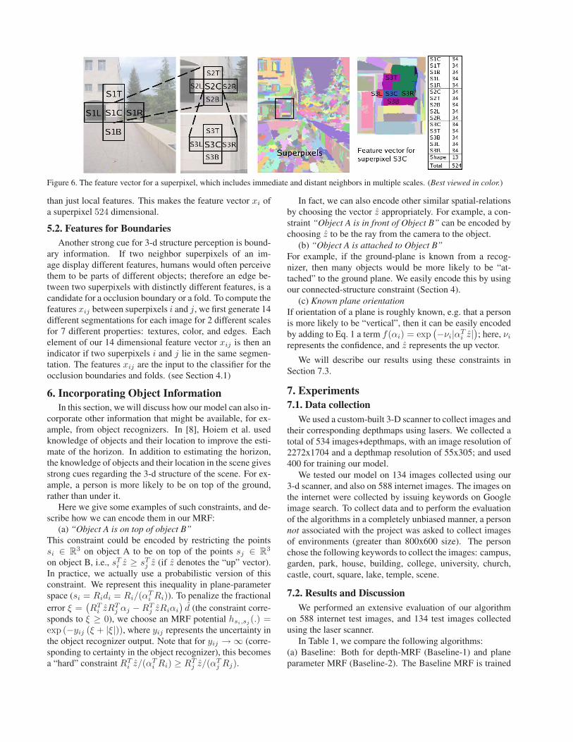
Figure 6. The feature vector for a superpixel, which includes immediate and distant neighbors in multiple scales. (Best viewed in color.)

than just local features. This makes the feature vector xi ofa superpixel 524 dimensional.

5.2. Features for BoundariesAnother strong cue for 3-d structure perception is bound-

ary information. If two neighbor superpixels of an im-age display different features, humans would often perceivethem to be parts of different objects; therefore an edge be-tween two superpixels with distinctly different features, is acandidate for a occlusion boundary or a fold. To compute thefeatures xij between superpixels i and j, we first generate 14different segmentations for each image for 2 different scalesfor 7 different properties: textures, color, and edges. Eachelement of our 14 dimensional feature vector xij is then anindicator if two superpixels i and j lie in the same segmen-tation. The features xij are the input to the classifier for theocclusion boundaries and folds. (see Section 4.1)

6. Incorporating Object InformationIn this section, we will discuss how our model can also in-

corporate other information that might be available, for ex-ample, from object recognizers. In [8], Hoiem et al. usedknowledge of objects and their location to improve the esti-mate of the horizon. In addition to estimating the horizon,the knowledge of objects and their location in the scene givesstrong cues regarding the 3-d structure of the scene. For ex-ample, a person is more likely to be on top of the ground,rather than under it.

Here we give some examples of such constraints, and de-scribe how we can encode them in our MRF:

(a) “Object A is on top of object B”This constraint could be encoded by restricting the pointssi ∈ R

3 on object A to be on top of the points sj ∈ R3

on object B, i.e., sTi z ≥ sT

j z (if z denotes the “up” vector).In practice, we actually use a probabilistic version of thisconstraint. We represent this inequality in plane-parameterspace (si = Ridi = Ri/(αT

i Ri)). To penalize the fractionalerror ξ =

(RT

i zRTj αj −RT

j zRiαi

)d (the constraint corre-

sponds to ξ ≥ 0), we choose an MRF potential hsi,sj(.) =

exp (−yij (ξ + |ξ|)), where yij represents the uncertainty inthe object recognizer output. Note that for yij → ∞ (corre-sponding to certainty in the object recognizer), this becomesa “hard” constraint RT

i z/(αTi Ri) ≥ RT

j z/(αTj Rj).

In fact, we can also encode other similar spatial-relationsby choosing the vector z appropriately. For example, a con-straint “Object A is in front of Object B” can be encoded bychoosing z to be the ray from the camera to the object.

(b) “Object A is attached to Object B”For example, if the ground-plane is known from a recog-nizer, then many objects would be more likely to be “at-tached” to the ground plane. We easily encode this by usingour connected-structure constraint (Section 4).

(c) Known plane orientationIf orientation of a plane is roughly known, e.g. that a personis more likely to be “vertical”, then it can be easily encodedby adding to Eq. 1 a term f(αi) = exp

(−νi|αTi z|

); here, νi

represents the confidence, and z represents the up vector.

We will describe our results using these constraints inSection 7.3.

7. Experiments7.1. Data collection

We used a custom-built 3-D scanner to collect images andtheir corresponding depthmaps using lasers. We collected atotal of 534 images+depthmaps, with an image resolution of2272x1704 and a depthmap resolution of 55x305; and used400 for training our model.

We tested our model on 134 images collected using our3-d scanner, and also on 588 internet images. The images onthe internet were collected by issuing keywords on Googleimage search. To collect data and to perform the evaluationof the algorithms in a completely unbiased manner, a personnot associated with the project was asked to collect imagesof environments (greater than 800x600 size). The personchose the following keywords to collect the images: campus,garden, park, house, building, college, university, church,castle, court, square, lake, temple, scene.

7.2. Results and DiscussionWe performed an extensive evaluation of our algorithm

on 588 internet test images, and 134 test images collectedusing the laser scanner.

In Table 1, we compare the following algorithms:(a) Baseline: Both for depth-MRF (Baseline-1) and planeparameter MRF (Baseline-2). The Baseline MRF is trained

Figure 7. (a) Original Image, (b) Ground truth depthmap, (c) Depth from image features only, (d) Point-wise MRF, (e) Plane parameterMRF. (Best viewed in Color)Table 1. Results: Quantitative comparison of various methods.

METHOD CORRECT % PLANES log10 REL

(%) CORRECT

SCN NA NA 0.198 0.530HEH 33.1% 50.3% 0.320 1.423BASELINE-1 0% NA 0.300 0.698NO PRIORS 0% NA 0.170 0.447POINT-WISE MRF 23% NA 0.149 0.458BASELINE-2 0% 0% 0.334 0.516NO PRIORS 0% 0% 0.205 0.392CO-PLANAR 45.7% 57.1% 0.191 0.373PP-MRF 64.9% 71.2% 0.187 0.370

without any image features, and thus reflects a “prior”depthmap of sorts.(b) Our Point-wise MRF: with and without constraints (con-nectivity, co-planar and co-linearity).(c) Our Plane Parameter MRF (PP-MRF): without any con-straint, with co-planar constraint only, and the full model.(d) Saxena et al. (SCN), applicable for quantitative errors.(e) Hoiem et al. (HEH). For fairness, we scale and shift theirdepthmaps before computing the errors to match the globalscale of our test images. Without the scaling and shifting,their error is much higher (7.533 for relative depth error).

We compare the algorithms on the following metrics: (a)Average depth error on a log-10 scale, (b) Average relativedepth error, (We give these numerical errors on only the 134test images that we collected, because ground-truth depthsare not available for internet images.) (c) % of models qual-itatively correct, (d) % of major planes correctly identified.3

Table 1 shows that both of our models (Point-wise MRFand Plane Parameter MRF) outperform both SCN and HEHin quantitative accuracy in depth prediction. Plane Parame-ter MRF gives better relative depth accuracy, and producessharper depthmaps. (Fig. 7) Table 1 also shows that by cap-turing the image properties of connected structure, copla-narity and colinearity, the models produced by the algorithmbecome significantly better. In addition to reducing quan-titative errors, PP-MRF does indeed produce significantlybetter 3-d models. When producing 3-d flythroughs, even asmall number of erroneous planes make the 3-d model vi-sually unacceptable, even though the quantitative numbers

3We define a model as correct when for 70% of the major planes in theimage (major planes occupy more than 15% of the area), the plane is incorrect relationship with its nearest neighbors (i.e., the relative orientationof the planes is within 30 degrees). Note that changing the numbers, suchas 70% to 50% or 90%, 15% to 10% or 30%, and 30 degrees to 20 or 45degrees, gave similar trends in the results.

Table 2. Percentage of images for which HEH is better, our PP-MRF is better, or it is a tie.

ALGORITHM %BETTER

TIE 15.8%HEH 22.1%PP-MRF 62.1%

may still show small errors.Our algorithm gives qualitatively correct models for

64.9% of images as compared to 33.1% by HEH. The qual-itative evaluation was performed by a person not associ-ated with the project following the guidelines in Footnote 3.HEH generate a “photo-popup” effect by folding the im-ages at “ground-vertical” boundaries—an assumption whichis not true for a significant number of images; therefore, theirmethod fails in those images. Some typical examples of the3-d models are shown in Fig. 8. (Note that all the test casesshown in Fig. 1, 8 and 9 are from the dataset downloadedfrom the internet, except Fig. 9a which is from the laser-testdataset.) These examples also show that our models are of-ten more detailed than HEH, in that they are often able tomodel the scene with a multitude (over a hundred) of planes.

We performed a further comparison to HEH. Even whenboth HEH and our algorithm is evaluated as qualitativelycorrect on an image, one result could still be superior. There-fore, we asked the person to compare the two methods, anddecide which one is better, or is a tie.4 Table 2 shows that ouralgorithm performs better than HEH in 62.1% of the cases.Full documentation describing the details of the unbiasedhuman judgment process, along with the 3-d flythroughsproduced by our algorithm and HEH, is available online at:

http://ai.stanford.edu/∼asaxena/reconstruction3dSome of our models, e.g. in Fig. 9j, have cosmetic

defects—e.g. stretched texture; better texture rendering tech-niques would make the models more visually pleasing. Insome cases, a small mistake (i.e., one person being detectedas far-away in Fig. 9h) makes the model look bad; and hencebe evaluated as “incorrect.”

Our algorithm, trained on images taken in a smallgeographical area in our university, was able to predict

4To compare the algorithms, the person was asked to count the numberof errors made by each algorithm. We define an error when a major plane inthe image (occupying more than 15% area in the image) is in wrong locationwith respect to its neighbors, or if the orientation of the plane is more than30 degrees wrong. For example, if HEH fold the image at incorrect place(see Fig. 8, image 2), then it is counted as an error. Similarly, if we predicttop of a building as far and the bottom part of building near, making thebuilding tilted—it would count as an error.

Figure 8. Typical results from HEH and our algorithm. Row 1: Original Image. Row 2: 3-d model generated by HEH, Row 3 and4: 3-d model generated by our algorithm. (Note that the screenshots cannot be simply obtained from the original image by an affinetransformation.) In image 1, HEH makes mistakes in some parts of the foreground rock, while our algorithm predicts the correct model;with the rock occluding the house, giving a novel view. In image 2, HEH algorithm detects a wrong ground-vertical boundary; whileour algorithm not only finds the correct ground, but also captures a lot of non-vertical structure, such as the blue slide. In image 3, HEHis confused by the reflection; while our algorithm produces a correct 3-d model. In image 4, HEH and our algorithm produce roughlyequivalent results—HEH is a bit more visually pleasing and our model is a bit more detailed. In image 5, both HEH and our algorithm fail;HEH just predict one vertical plane at a incorrect location. Our algorithm predicts correct depths of the pole and the horse, but is unable todetect their boundary; hence making it qualitatively incorrect.

Figure 10. (Left) Original Images, (Middle) Snapshot of the 3-dmodel without using object information, (Right) Snapshot of the3-d model that uses object information.

qualitatively correct 3-d models for a large variety ofenvironments—for example, ones that have hills, lakes, andones taken at night, and even paintings. (See Fig. 9 and thewebsite.) We believe, based on our experiments varying thenumber of training examples (not reported here), that hav-ing a larger and more diverse set of training images wouldimprove the algorithm significantly.

7.3. Results using Object InformationWe also performed experiments in which information

from object recognizers was incorporated into the MRF forinferring a 3-d model (Section 6). In particular, we im-plemented a recognizer (based on the features described inSection 5) for ground-plane, and used the Dalal-Triggs De-tector [2] to detect pedestrains. For these objects, we en-coded the (a), (b) and (c) constraints described in Section 6.Fig. 10 shows that using the pedestrian and ground detectorimproves the accuracy of the 3-d model. Also note that using“soft” constraints in the MRF (Section 6), instead of “hard”constraints, helps in estimating correct 3-d models even ifthe object recognizer makes a mistake.

8. ConclusionsWe presented an algorithm for inferring detailed 3-d

structure from a single still image. Compared to previ-ous approaches, our model creates 3-d models which areboth quantitatively more accurate and more visually pleas-ing. We model both the location and orientation of small

Figure 9. Typical results from our algorithm. Original image (top), and a screenshot of the 3-d flythrough generated from the image (bottomof the image). The first 7 images (a-g) were evaluated as “correct” and the last 3 (h-j) were evaluated as “incorrect.”

homogenous regions in the image, called “superpixels,” us-ing an MRF. Our model, trained via supervised learning,estimates plane parameters using image features, and alsoreasons about relationships between various parts of the im-age. MAP inference for our model is efficiently performedby solving a linear program. Other than assuming thatthe environment is made of a number of small planes, wedo not make any explicit assumptions about the structureof the scene, such as the “ground-vertical” planes assump-tion by Delage et al. and Hoiem et al.; thus our model isable to generalize well, even to scenes with significant non-vertical structure. We created visually pleasing 3-d modelsautonomously for 64.9% of the 588 internet images, as com-pared to Hoiem et al.’s performance of 33.1%. Our modelsare also quantitatively more accurate than prior art. Finally,we also extended our model to incorporate information fromobject recognizers to produce better 3-d models.

Acknowledgments: We thank Rajiv Agarwal and Jamie Schulte forhelp in collecting data. We also thank James Diebel, Jeff Michels andAlyosha Efros for helpful discussions. This work was supported by theNational Science Foundation under award CNS-0551737, and by the Officeof Naval Research under MURI N000140710747.

References[1] A. Criminisi, I. Reid, and A. Zisserman. Single view metrology. IJCV,

40:123–148, 2000.[2] N. Dalai and B. Triggs. Histogram of oriented gradients for human

detection. In CVPR, 2005.

[3] E. Delage, H. Lee, and A. Ng. Automatic single-image 3d reconstruc-tions of indoor manhattan world scenes. In ISRR, 2005.

[4] E. Delage, H. Lee, and A. Y. Ng. A dynamic bayesian network modelfor autonomous 3d reconstruction from a single indoor image. InCVPR, 2006.

[5] P. Felzenszwalb and D. Huttenlocher. Efficient graph-based imagesegmentation. IJCV, 59, 2004.

[6] D. A. Forsyth and J. Ponce. Computer Vision : A Modern Approach.Prentice Hall, 2003.

[7] D. Hoiem, A. Efros, and M. Hebert. Automatic photo pop-up. InACM SIGGRAPH, 2005.

[8] D. Hoiem, A. Efros, and M. Hebert. Putting objects in perspective. InCVPR, 2006.

[9] D. Hoiem, A. Efros, and M. Herbert. Geometric context from a singleimage. In ICCV, 2005.

[10] R. Koch, M. Pollefeys, and L. V. Gool. Multi viewpoint stereo fromuncalibrated video sequences. In ECCV, 1998.

[11] A. McCalloum, C. Pal, G. Druck, and X. Wang. Multi-conditionallearning: generative/discriminative training for clustering and classi-fication. In AAAI, 2006.

[12] J. Michels, A. Saxena, and A. Y. Ng. High speed obstacle avoidanceusing monocular vision & reinforcement learning. In ICML, 2005.

[13] A. Saxena, S. H. Chung, and A. Y. Ng. Learning depth from singlemonocular images. In NIPS 18, 2005.

[14] A. Saxena, S. H. Chung, and A. Y. Ng. 3-d depth reconstruction froma single still image. IJCV, 2007.

[15] A. Saxena, J. Schulte, and A. Y. Ng. Depth estimation using monoc-ular and stereo cues. In IJCAI, 2007.

[16] D. Scharstein and R. Szeliski. A taxonomy and evaluation of densetwo-frame stereo correspondence algorithms. IJCV, 47, 2002.

[17] B. A. Wandell. Foundations of Vision. Sinauer Associates, Sunder-land, MA, 1995.

[18] R. Zhang, P. Tsai, J. Cryer, and M. Shah. Shape from shading: Asurvey. IEEE PAMI, 21:690–706, 1999.