leaf conjugacies on the torus - instituto nacional de ...w3.impa.br/~andy/slides/uofa-talk.pdf ·...
TRANSCRIPT
Leaf conjugacies on the torus
Andy Hammerlindl
University of Toronto
June 22, 2009
1
Hyperbolic Systems
•Diffeomorphism f : M → M on a Riemannian manifold M .
2
Hyperbolic Systems
•Diffeomorphism f : M → M on a Riemannian manifold M .
•Tf -invariant splitting:
TM = Eu ⊕ Es
2
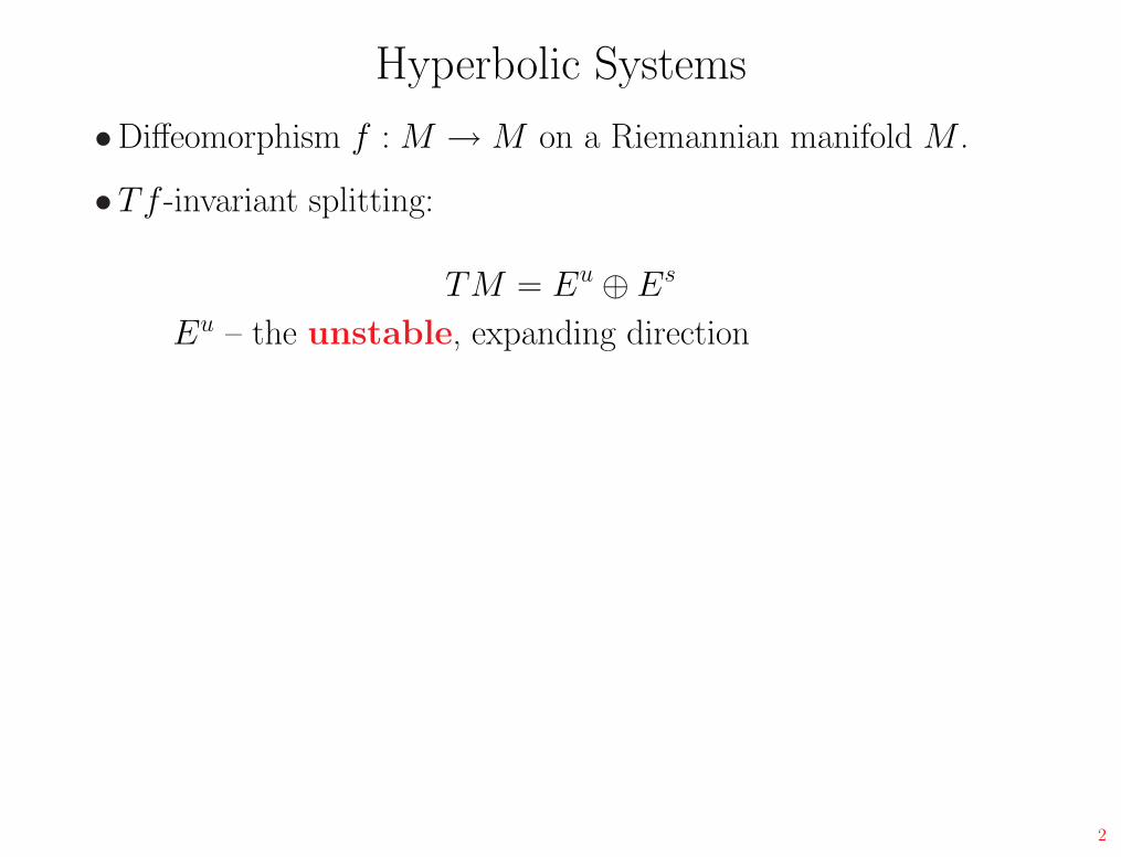
Hyperbolic Systems
•Diffeomorphism f : M → M on a Riemannian manifold M .
•Tf -invariant splitting:
TM = Eu ⊕ Es
Eu – the unstable, expanding direction
2
Hyperbolic Systems
•Diffeomorphism f : M → M on a Riemannian manifold M .
•Tf -invariant splitting:
TM = Eu ⊕ Es
Eu – the unstable, expanding direction
Es – the stable, contracting direction
2

Hyperbolic Systems
•Diffeomorphism f : M → M on a Riemannian manifold M .
•Tf -invariant splitting:
TM = Eu ⊕ Es
Eu – the unstable, expanding direction
Es – the stable, contracting direction
•There are constants λ < 1 < µ such that
2
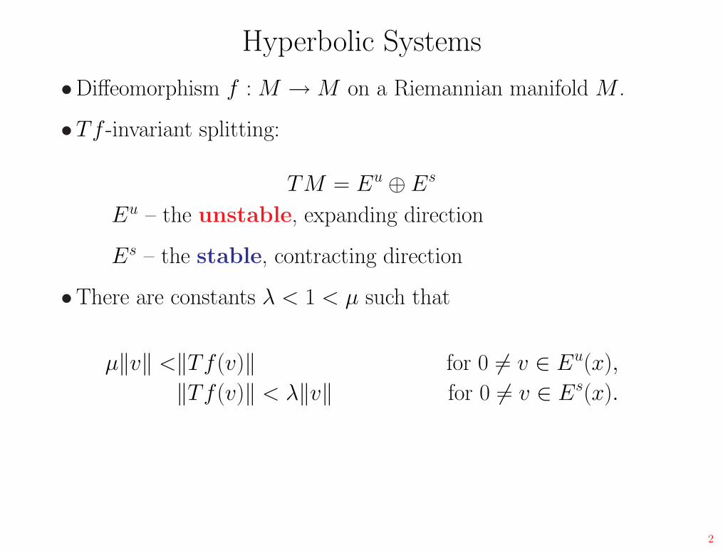
Hyperbolic Systems
•Diffeomorphism f : M → M on a Riemannian manifold M .
•Tf -invariant splitting:
TM = Eu ⊕ Es
Eu – the unstable, expanding direction
Es – the stable, contracting direction
•There are constants λ < 1 < µ such that
µ‖v‖ <‖Tf(v)‖ for 0 6= v ∈ Eu(x),
‖Tf(v)‖ < λ‖v‖ for 0 6= v ∈ Es(x).
2
Hyperbolic Systems
•Diffeomorphism f : M → M on a Riemannian manifold M .
•Tf -invariant splitting:
TM = Eu ⊕ Es
Eu – the unstable, expanding direction
Es – the stable, contracting direction
•There are constants λ < 1 < µ such that
µ‖v‖ <‖Tf(v)‖ for 0 6= v ∈ Eu(x),
‖Tf(v)‖ < λ‖v‖ for 0 6= v ∈ Es(x).
1
us
2

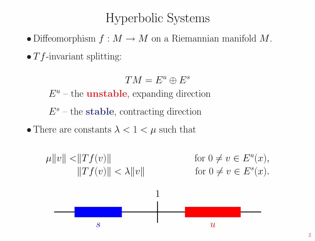
Hyperbolic Systems
•Diffeomorphism f : M → M on a Riemannian manifold M .
•Tf -invariant splitting:
TM = Eu ⊕ Es
Eu – the unstable, expanding direction
Es – the stable, contracting direction
•There are constants λ < 1 < µ such that
µ‖v‖ <‖Tf(v)‖ for 0 6= v ∈ Eu(x),
‖Tf(v)‖ < λ‖v‖ for 0 6= v ∈ Es(x).
1
us
µλ
2
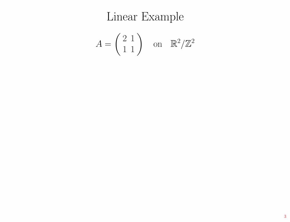
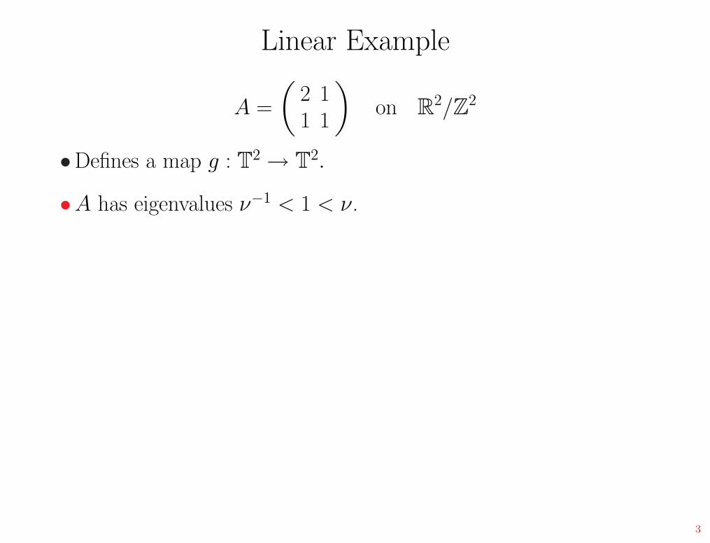
Linear Example
A =
(
2 11 1
)
on R2/Z
2
3

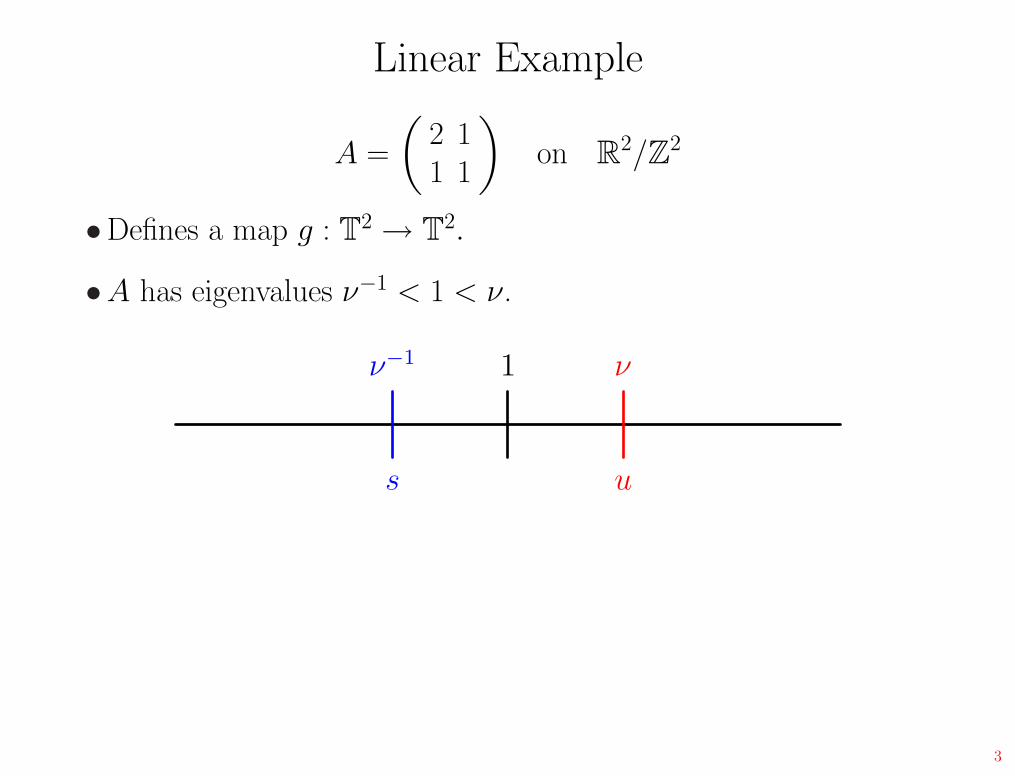
Linear Example
A =
(
2 11 1
)
on R2/Z
2
•Defines a map g : T2 → T
2.
3
Linear Example
A =
(
2 11 1
)
on R2/Z
2
•Defines a map g : T2 → T
2.
•A has eigenvalues ν−1 < 1 < ν.
3
Linear Example
A =
(
2 11 1
)
on R2/Z
2
•Defines a map g : T2 → T
2.
•A has eigenvalues ν−1 < 1 < ν.
1 ν
u
ν−1
s
3
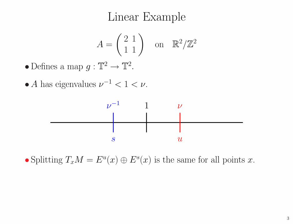
Linear Example
A =
(
2 11 1
)
on R2/Z
2
•Defines a map g : T2 → T
2.
•A has eigenvalues ν−1 < 1 < ν.
1 ν
u
ν−1
s
• Splitting TxM = Eu(x) ⊕ Es(x) is the same for all points x.
3
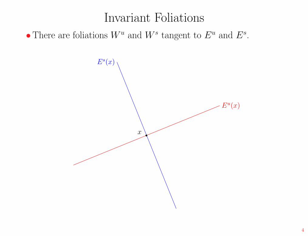
Invariant Foliations
•There are foliations W u and W s tangent to Eu and Es.
Eu(x)
Es(x)
x
4
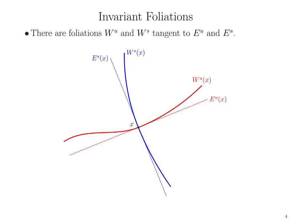
Invariant Foliations
•There are foliations W u and W s tangent to Eu and Es.
Eu(x)
Es(x)
x
W u(x)
W s(x)
4

Invariant Foliations
• If x and y lie on the same stable leaf, then
ds
(
f(x), f(y))
< λ ds(x, y)
Here, ds denotes distance along the leaf.
5
Invariant Foliations
• If x and y lie on the same stable leaf, then
ds
(
f(x), f(y))
< λ ds(x, y)
Here, ds denotes distance along the leaf.
•For k ∈ Z,
ds
(
fk(x), fk(y))
< λk ds(x, y).
5
Invariant Foliations
• If x and y lie on the same stable leaf, then
ds
(
f(x), f(y))
< λ ds(x, y)
Here, ds denotes distance along the leaf.
•For k ∈ Z,
ds
(
fk(x), fk(y))
< λk ds(x, y).
• Similarly, if x, y lie on the same unstable leaf, then
µk du(x, y) < du
(
fk(x), fk(y))
.
5
Franks and Manning
•Every hyperbolic f : Td → T
d is conjugate to a linear toralautomorphism g : T
d → Td.
6
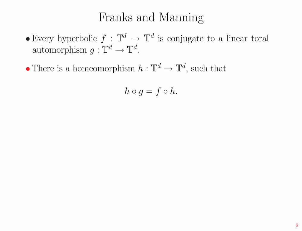
Franks and Manning
•Every hyperbolic f : Td → T
d is conjugate to a linear toralautomorphism g : T
d → Td.
•There is a homeomorphism h : Td → T
d, such that
h ◦ g = f ◦ h.
6
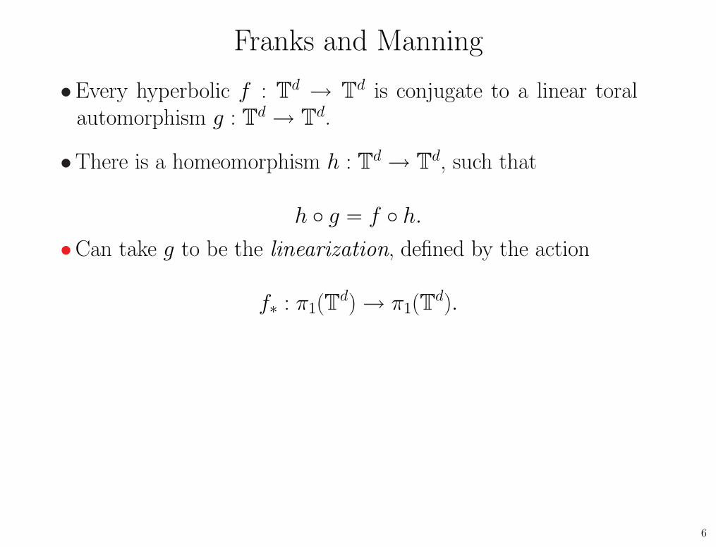
Franks and Manning
•Every hyperbolic f : Td → T
d is conjugate to a linear toralautomorphism g : T
d → Td.
•There is a homeomorphism h : Td → T
d, such that
h ◦ g = f ◦ h.
•Can take g to be the linearization, defined by the action
f∗ : π1(Td) → π1(T
d).
6
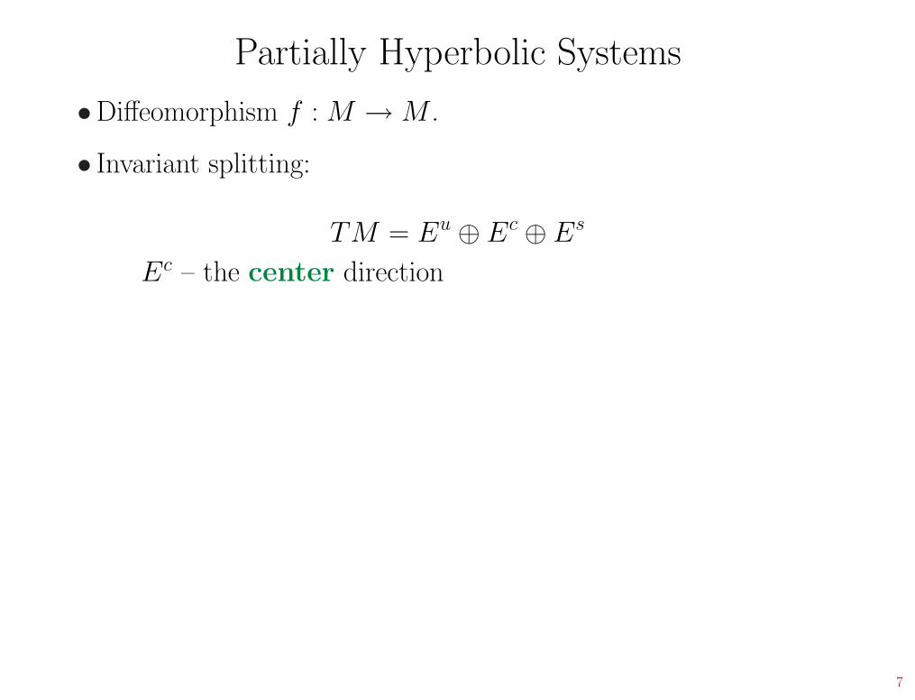
Partially Hyperbolic Systems
•Diffeomorphism f : M → M .
7
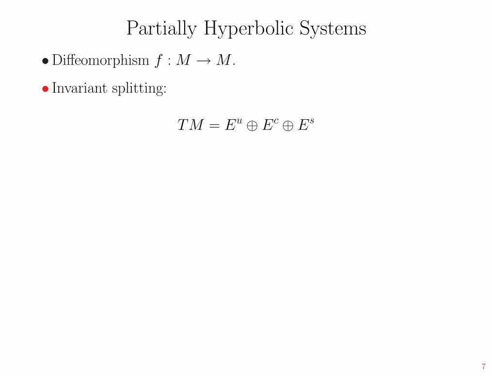
Partially Hyperbolic Systems
•Diffeomorphism f : M → M .
• Invariant splitting:
TM = Eu ⊕ Ec ⊕ Es
7
Partially Hyperbolic Systems
•Diffeomorphism f : M → M .
• Invariant splitting:
TM = Eu ⊕ Ec ⊕ Es
Ec – the center direction
7
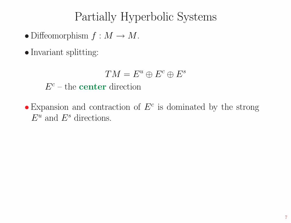
Partially Hyperbolic Systems
•Diffeomorphism f : M → M .
• Invariant splitting:
TM = Eu ⊕ Ec ⊕ Es
Ec – the center direction
•Expansion and contraction of Ec is dominated by the strongEu and Es directions.
7
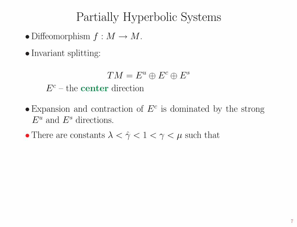
Partially Hyperbolic Systems
•Diffeomorphism f : M → M .
• Invariant splitting:
TM = Eu ⊕ Ec ⊕ Es
Ec – the center direction
•Expansion and contraction of Ec is dominated by the strongEu and Es directions.
•There are constants λ < γ̂ < 1 < γ < µ such that
7
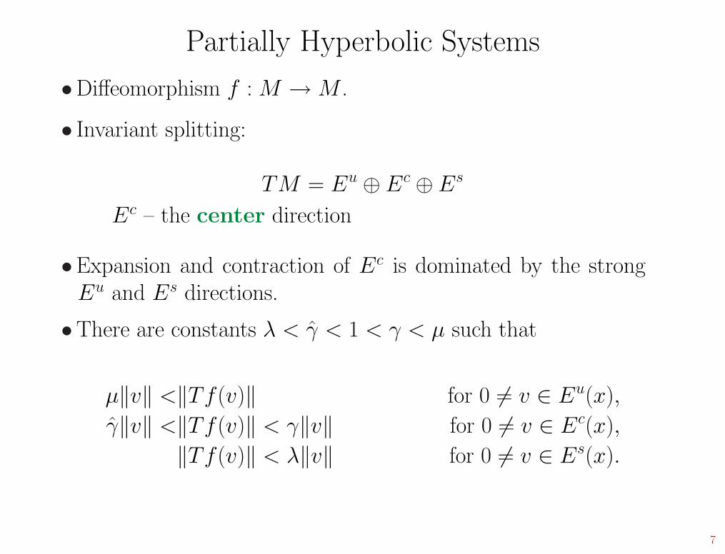
Partially Hyperbolic Systems
•Diffeomorphism f : M → M .
• Invariant splitting:
TM = Eu ⊕ Ec ⊕ Es
Ec – the center direction
•Expansion and contraction of Ec is dominated by the strongEu and Es directions.
•There are constants λ < γ̂ < 1 < γ < µ such that
µ‖v‖ <‖Tf(v)‖ for 0 6= v ∈ Eu(x),
γ̂‖v‖ <‖Tf(v)‖ < γ‖v‖ for 0 6= v ∈ Ec(x),
‖Tf(v)‖ < λ‖v‖ for 0 6= v ∈ Es(x).
7
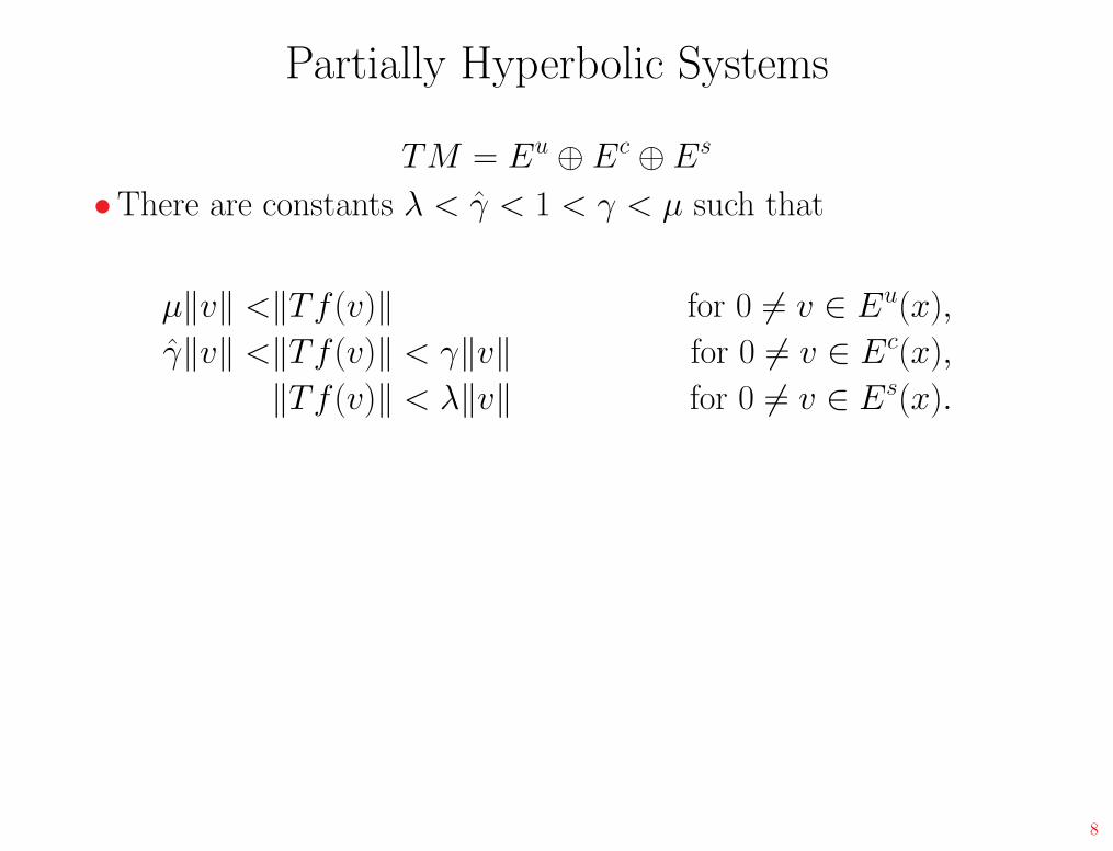
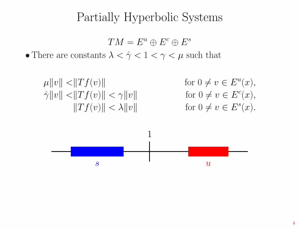
Partially Hyperbolic Systems
TM = Eu ⊕ Ec ⊕ Es
•There are constants λ < γ̂ < 1 < γ < µ such that
µ‖v‖ <‖Tf(v)‖ for 0 6= v ∈ Eu(x),
γ̂‖v‖ <‖Tf(v)‖ < γ‖v‖ for 0 6= v ∈ Ec(x),
‖Tf(v)‖ < λ‖v‖ for 0 6= v ∈ Es(x).
8
Partially Hyperbolic Systems
TM = Eu ⊕ Ec ⊕ Es
•There are constants λ < γ̂ < 1 < γ < µ such that
µ‖v‖ <‖Tf(v)‖ for 0 6= v ∈ Eu(x),
γ̂‖v‖ <‖Tf(v)‖ < γ‖v‖ for 0 6= v ∈ Ec(x),
‖Tf(v)‖ < λ‖v‖ for 0 6= v ∈ Es(x).
1
us
8
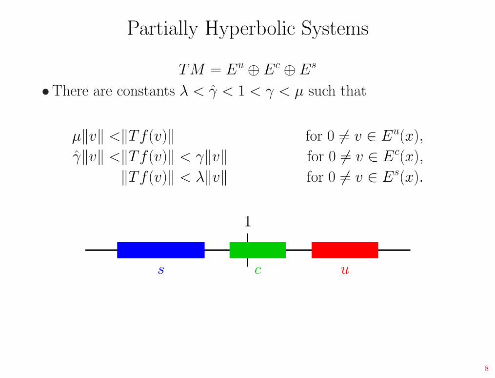
Partially Hyperbolic Systems
TM = Eu ⊕ Ec ⊕ Es
•There are constants λ < γ̂ < 1 < γ < µ such that
µ‖v‖ <‖Tf(v)‖ for 0 6= v ∈ Eu(x),
γ̂‖v‖ <‖Tf(v)‖ < γ‖v‖ for 0 6= v ∈ Ec(x),
‖Tf(v)‖ < λ‖v‖ for 0 6= v ∈ Es(x).
1
us c
8
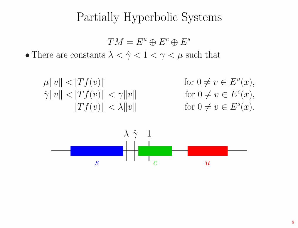
Partially Hyperbolic Systems
TM = Eu ⊕ Ec ⊕ Es
•There are constants λ < γ̂ < 1 < γ < µ such that
µ‖v‖ <‖Tf(v)‖ for 0 6= v ∈ Eu(x),
γ̂‖v‖ <‖Tf(v)‖ < γ‖v‖ for 0 6= v ∈ Ec(x),
‖Tf(v)‖ < λ‖v‖ for 0 6= v ∈ Es(x).
1
us c
λ γ̂
8
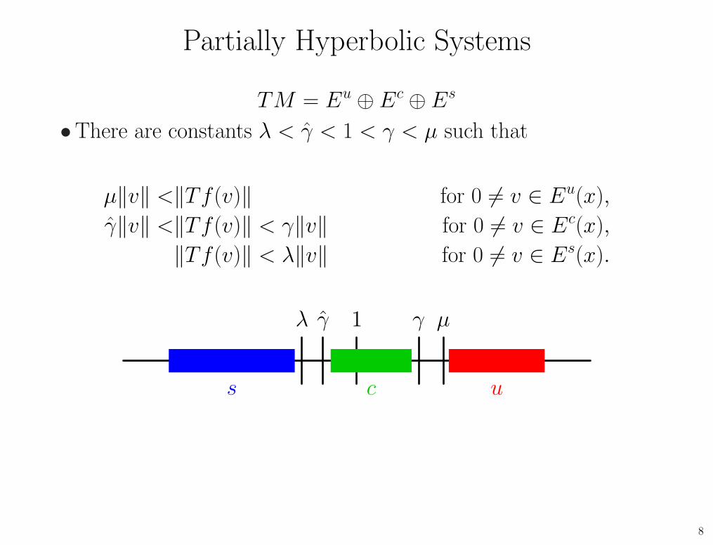
Partially Hyperbolic Systems
TM = Eu ⊕ Ec ⊕ Es
•There are constants λ < γ̂ < 1 < γ < µ such that
µ‖v‖ <‖Tf(v)‖ for 0 6= v ∈ Eu(x),
γ̂‖v‖ <‖Tf(v)‖ < γ‖v‖ for 0 6= v ∈ Ec(x),
‖Tf(v)‖ < λ‖v‖ for 0 6= v ∈ Es(x).
1
us c
λ γ̂ γ µ
8
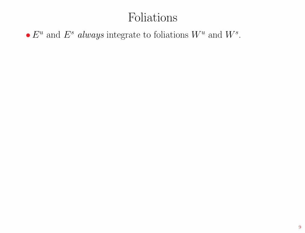
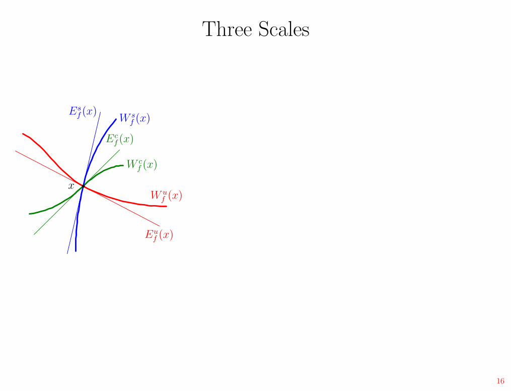
Foliations
•Eu and Es always integrate to foliations W u and W s.
9

Foliations
•Eu and Es always integrate to foliations W u and W s.
•Ec sometimes integrates to a foliation W c.
9
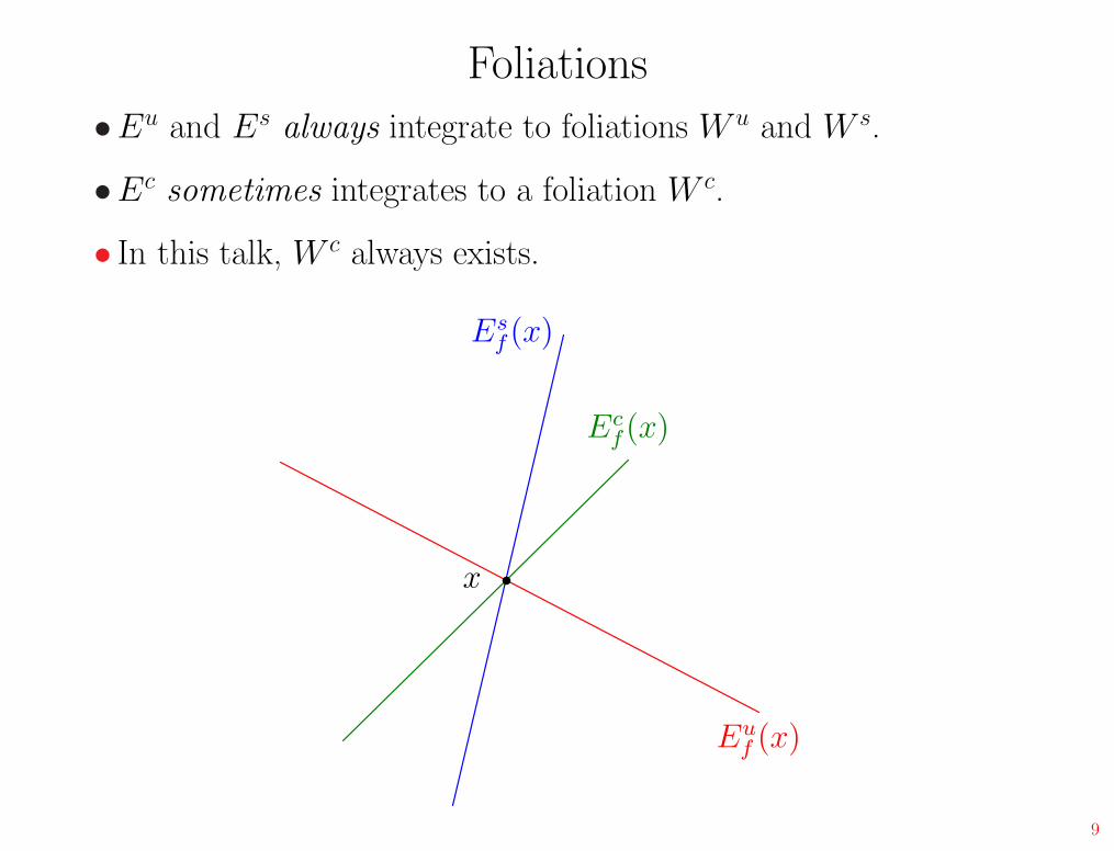
Foliations
•Eu and Es always integrate to foliations W u and W s.
•Ec sometimes integrates to a foliation W c.
• In this talk, W c always exists.
Euf (x)
Esf (x)
Ecf (x)
x
9

Foliations
•Eu and Es always integrate to foliations W u and W s.
•Ec sometimes integrates to a foliation W c.
• In this talk, W c always exists.
Euf (x)
Esf (x)
Ecf (x)
xW u
f (x)
W sf (x)
W cf (x)
9
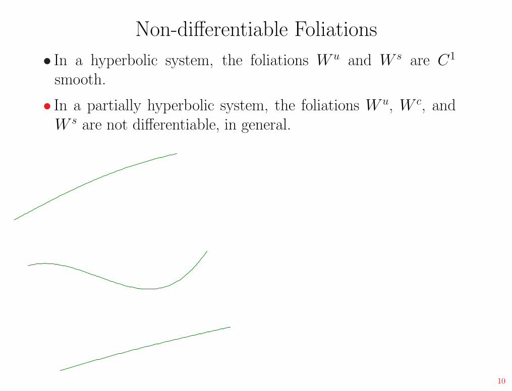
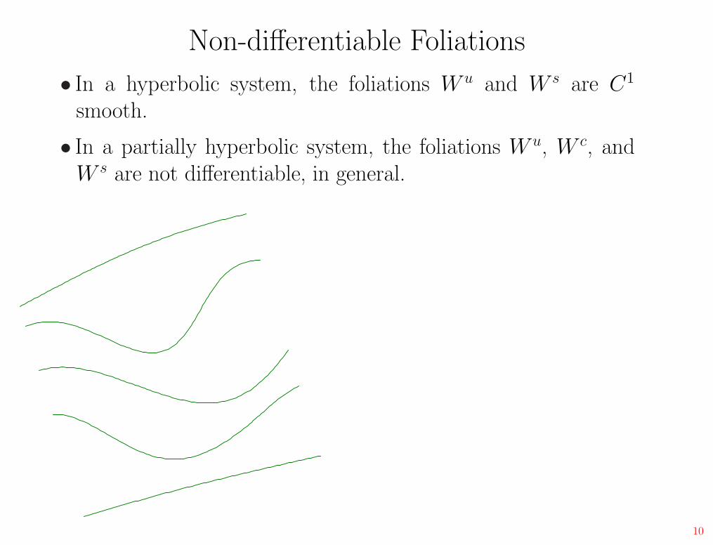
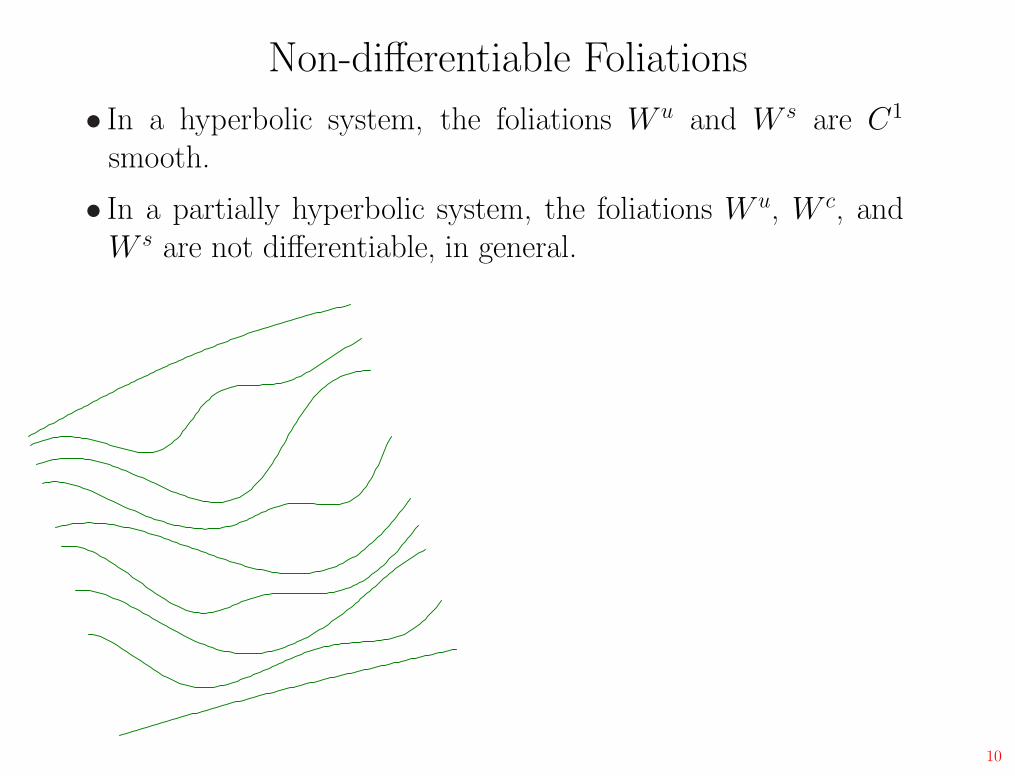
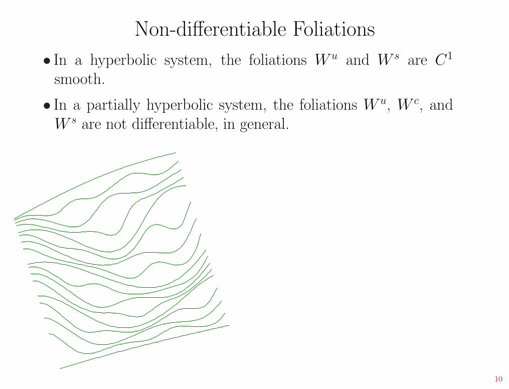
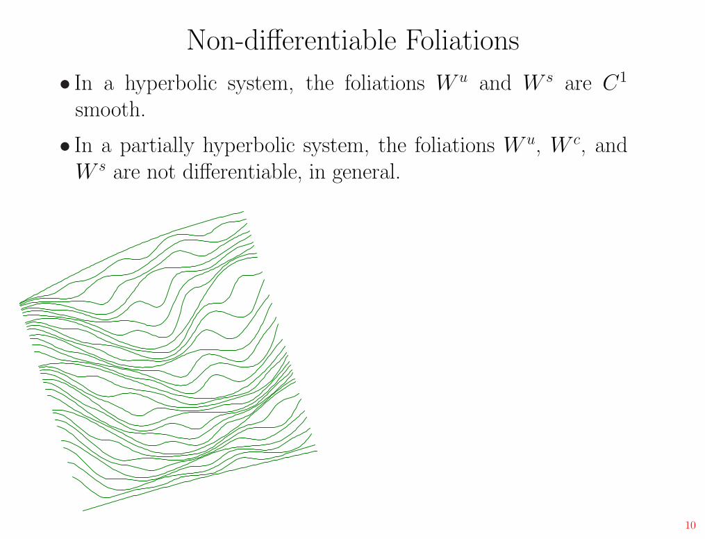
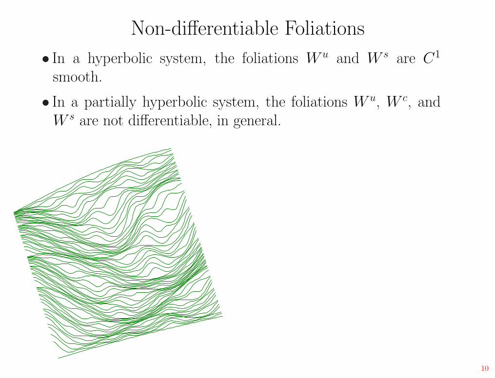
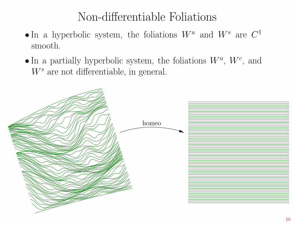
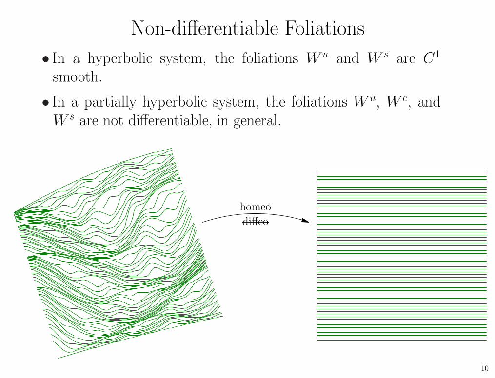
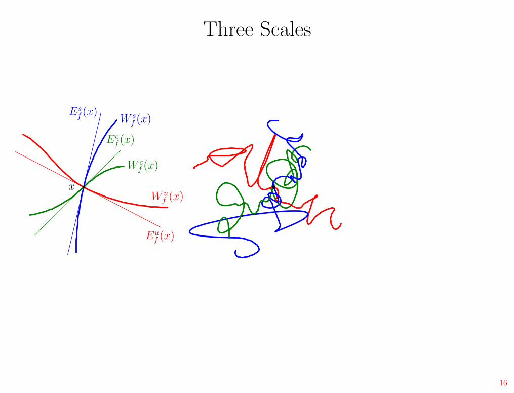
Non-differentiable Foliations
• In a hyperbolic system, the foliations W u and W s are C1
smooth.
10
Non-differentiable Foliations
• In a hyperbolic system, the foliations W u and W s are C1
smooth.
• In a partially hyperbolic system, the foliations W u, W c, andW s are not differentiable, in general.
10
Non-differentiable Foliations
• In a hyperbolic system, the foliations W u and W s are C1
smooth.
• In a partially hyperbolic system, the foliations W u, W c, andW s are not differentiable, in general.
10
Non-differentiable Foliations
• In a hyperbolic system, the foliations W u and W s are C1
smooth.
• In a partially hyperbolic system, the foliations W u, W c, andW s are not differentiable, in general.
10
Non-differentiable Foliations
• In a hyperbolic system, the foliations W u and W s are C1
smooth.
• In a partially hyperbolic system, the foliations W u, W c, andW s are not differentiable, in general.
10
Non-differentiable Foliations
• In a hyperbolic system, the foliations W u and W s are C1
smooth.
• In a partially hyperbolic system, the foliations W u, W c, andW s are not differentiable, in general.
10
Non-differentiable Foliations
• In a hyperbolic system, the foliations W u and W s are C1
smooth.
• In a partially hyperbolic system, the foliations W u, W c, andW s are not differentiable, in general.
10

Non-differentiable Foliations
• In a hyperbolic system, the foliations W u and W s are C1
smooth.
• In a partially hyperbolic system, the foliations W u, W c, andW s are not differentiable, in general.
10
Non-differentiable Foliations
• In a hyperbolic system, the foliations W u and W s are C1
smooth.
• In a partially hyperbolic system, the foliations W u, W c, andW s are not differentiable, in general.
homeo
10
Non-differentiable Foliations
• In a hyperbolic system, the foliations W u and W s are C1
smooth.
• In a partially hyperbolic system, the foliations W u, W c, andW s are not differentiable, in general.
homeo
diffeo
10
Leaf Conjugacy
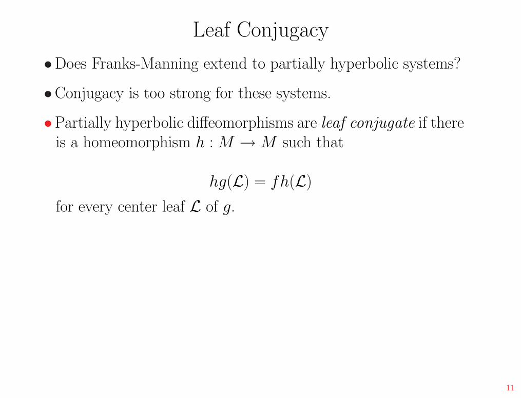
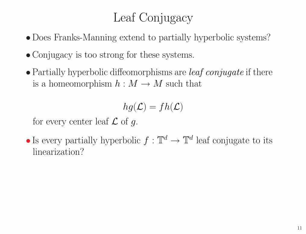
•Does Franks-Manning extend to partially hyperbolic systems?
11

Leaf Conjugacy
•Does Franks-Manning extend to partially hyperbolic systems?
•Conjugacy is too strong for these systems.
11
Leaf Conjugacy
•Does Franks-Manning extend to partially hyperbolic systems?
•Conjugacy is too strong for these systems.
•Partially hyperbolic diffeomorphisms are leaf conjugate if thereis a homeomorphism h : M → M such that
hg(L) = fh(L)
for every center leaf L of g.
11
Leaf Conjugacy
•Does Franks-Manning extend to partially hyperbolic systems?
•Conjugacy is too strong for these systems.
•Partially hyperbolic diffeomorphisms are leaf conjugate if thereis a homeomorphism h : M → M such that
hg(L) = fh(L)
for every center leaf L of g.
• Is every partially hyperbolic f : Td → T
d leaf conjugate to itslinearization?
11
The 3-torus
•T3 is the simplest manifold supporting partially hyperbolic
diffeomorphisms.
12
The 3-torus
•T3 is the simplest manifold supporting partially hyperbolic
diffeomorphisms.
• f0 : T3 → T
3 lifts to f : R3 → R
3.
12
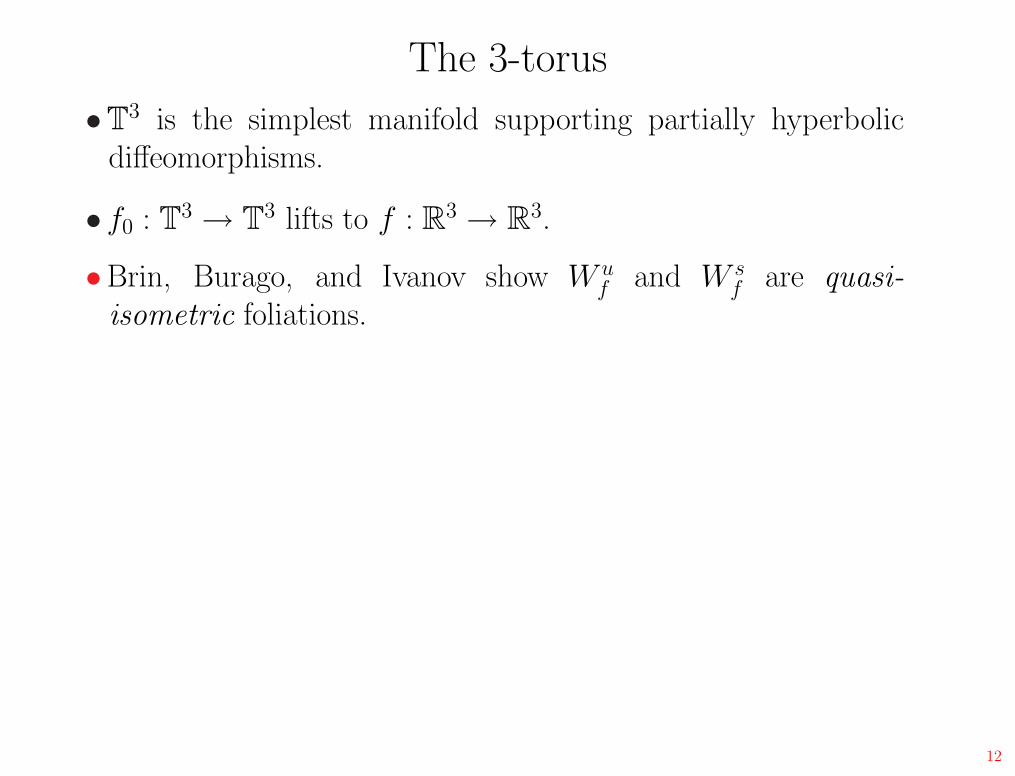
The 3-torus
•T3 is the simplest manifold supporting partially hyperbolic
diffeomorphisms.
• f0 : T3 → T
3 lifts to f : R3 → R
3.
•Brin, Burago, and Ivanov show W uf and W s
f are quasi-
isometric foliations.
12

The 3-torus
•T3 is the simplest manifold supporting partially hyperbolic
diffeomorphisms.
• f0 : T3 → T
3 lifts to f : R3 → R
3.
•Brin, Burago, and Ivanov show W uf and W s
f are quasi-
isometric foliations.
•For x and y on the same unstable leaf,
du(x, y) < Q · ‖x − y‖.
12

The 3-torus
•T3 is the simplest manifold supporting partially hyperbolic
diffeomorphisms.
• f0 : T3 → T
3 lifts to f : R3 → R
3.
•Brin, Burago, and Ivanov show W uf and W s
f are quasi-
isometric foliations.
•For x and y on the same unstable leaf,
du(x, y) < Q · ‖x − y‖.
•A leaf cannot return close to itself.
12
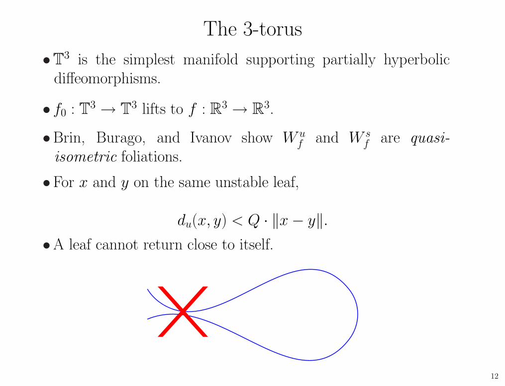
The 3-torus
•T3 is the simplest manifold supporting partially hyperbolic
diffeomorphisms.
• f0 : T3 → T
3 lifts to f : R3 → R
3.
•Brin, Burago, and Ivanov show W uf and W s
f are quasi-
isometric foliations.
•For x and y on the same unstable leaf,
du(x, y) < Q · ‖x − y‖.
•A leaf cannot return close to itself.
12
Main Theorem
Theorem. If f0 : Td → T
d is partially hyperbolic
13
Main Theorem
Theorem. If f0 : Td → T
d is partially hyperbolic
with lifting f : Rd → R
d,
13
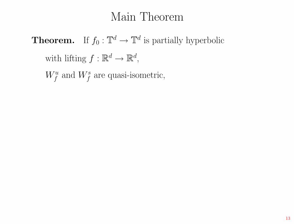
Main Theorem
Theorem. If f0 : Td → T
d is partially hyperbolic
with lifting f : Rd → R
d,
W uf and W s
f are quasi-isometric,
13
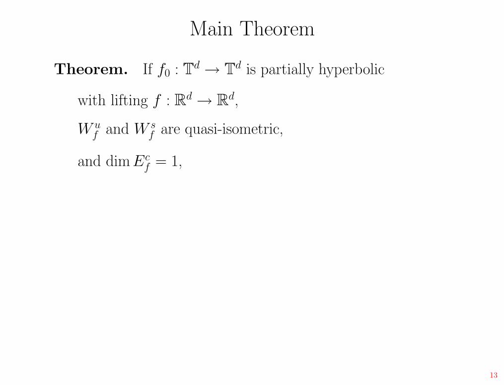
Main Theorem
Theorem. If f0 : Td → T
d is partially hyperbolic
with lifting f : Rd → R
d,
W uf and W s
f are quasi-isometric,
and dim Ecf = 1,
13
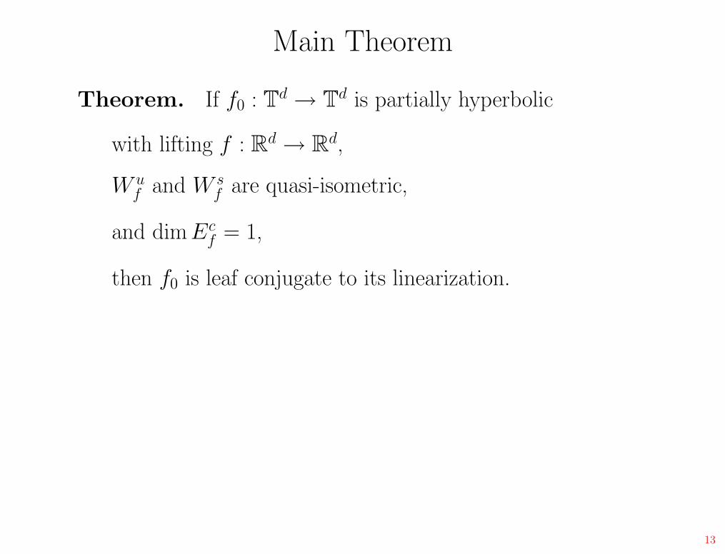
Main Theorem
Theorem. If f0 : Td → T
d is partially hyperbolic
with lifting f : Rd → R
d,
W uf and W s
f are quasi-isometric,
and dim Ecf = 1,
then f0 is leaf conjugate to its linearization.
13
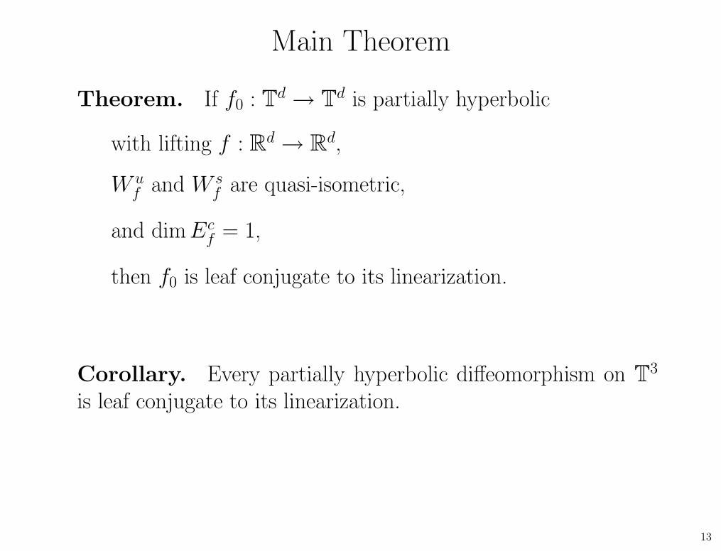
Main Theorem
Theorem. If f0 : Td → T
d is partially hyperbolic
with lifting f : Rd → R
d,
W uf and W s
f are quasi-isometric,
and dim Ecf = 1,
then f0 is leaf conjugate to its linearization.
Corollary. Every partially hyperbolic diffeomorphism on T3
is leaf conjugate to its linearization.
13
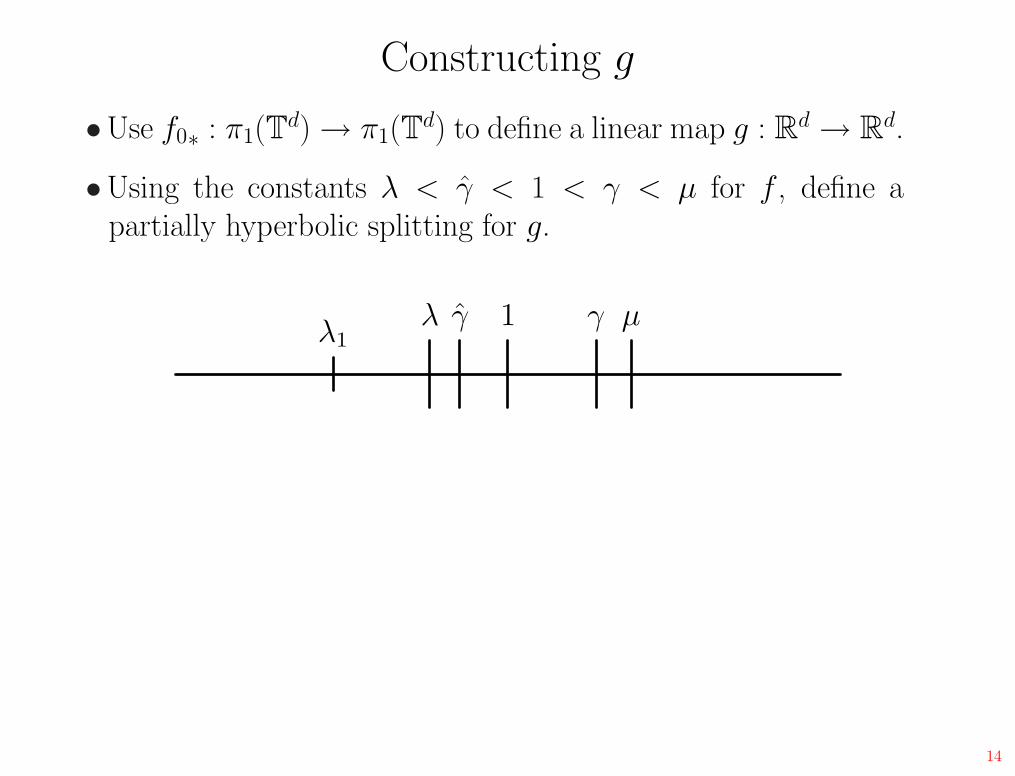
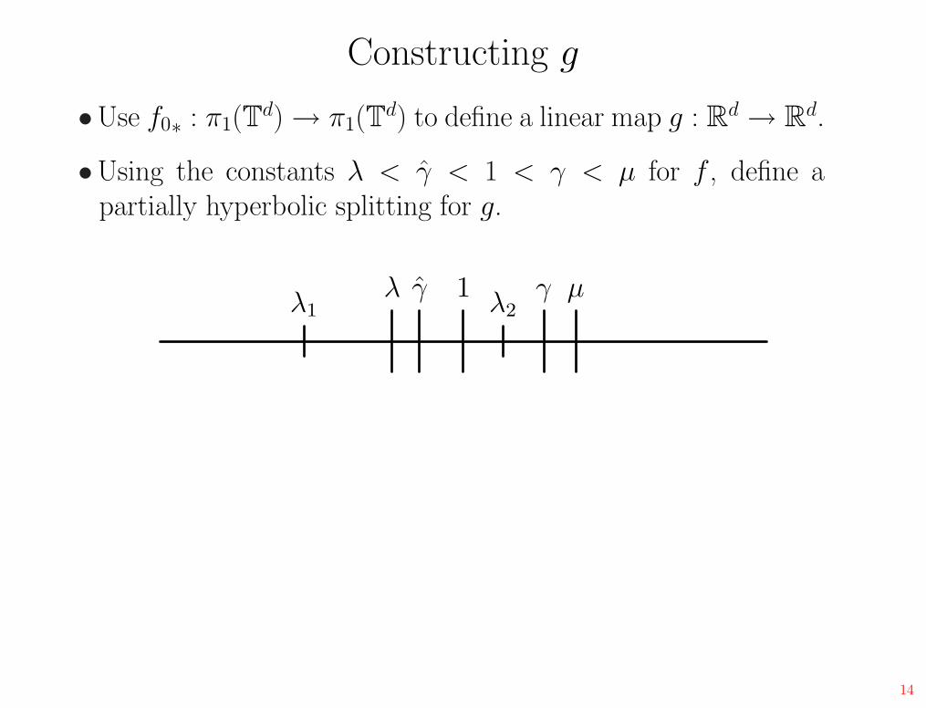
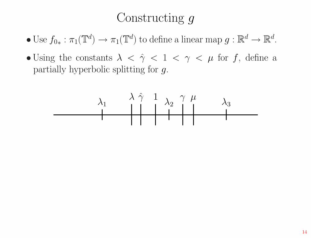
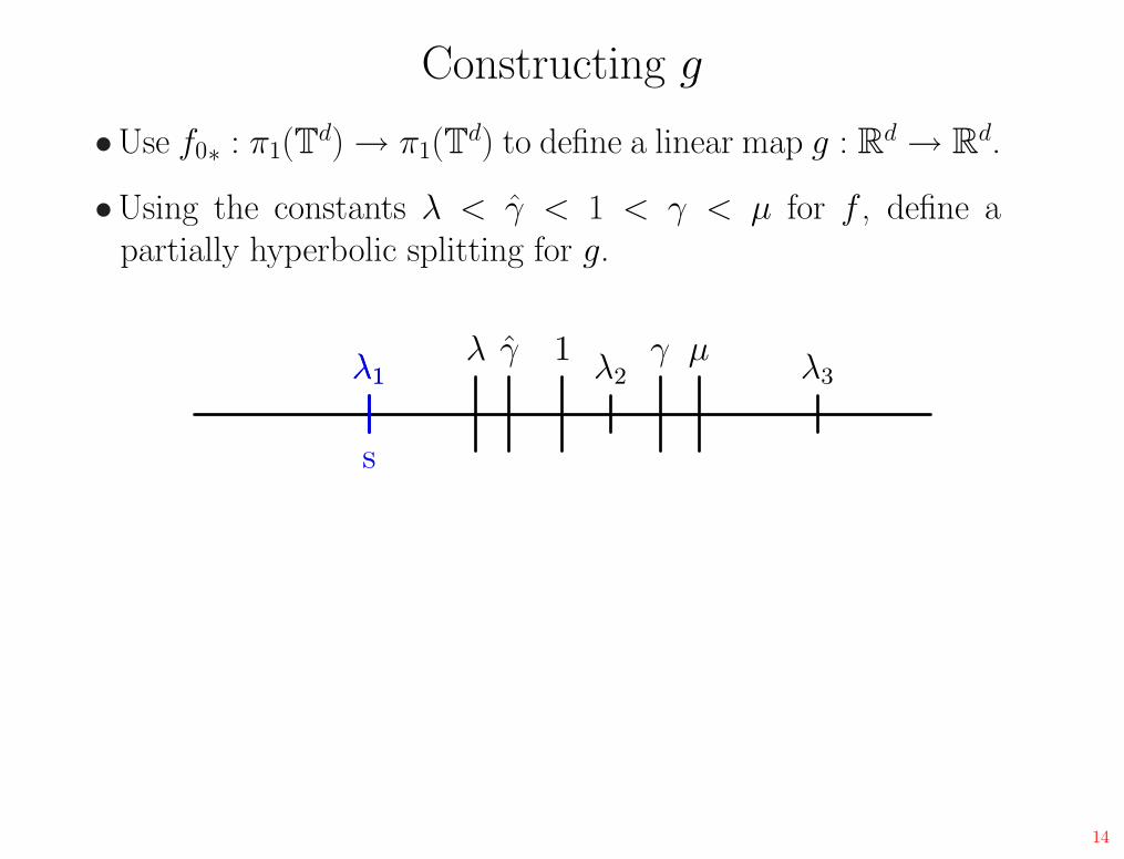
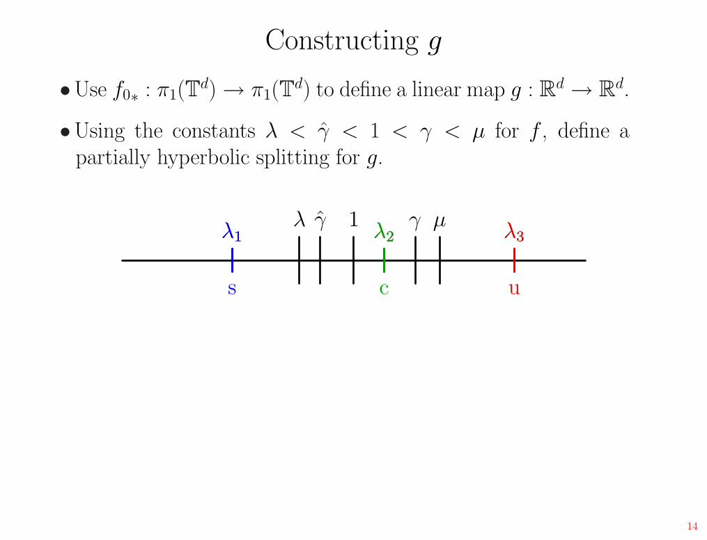
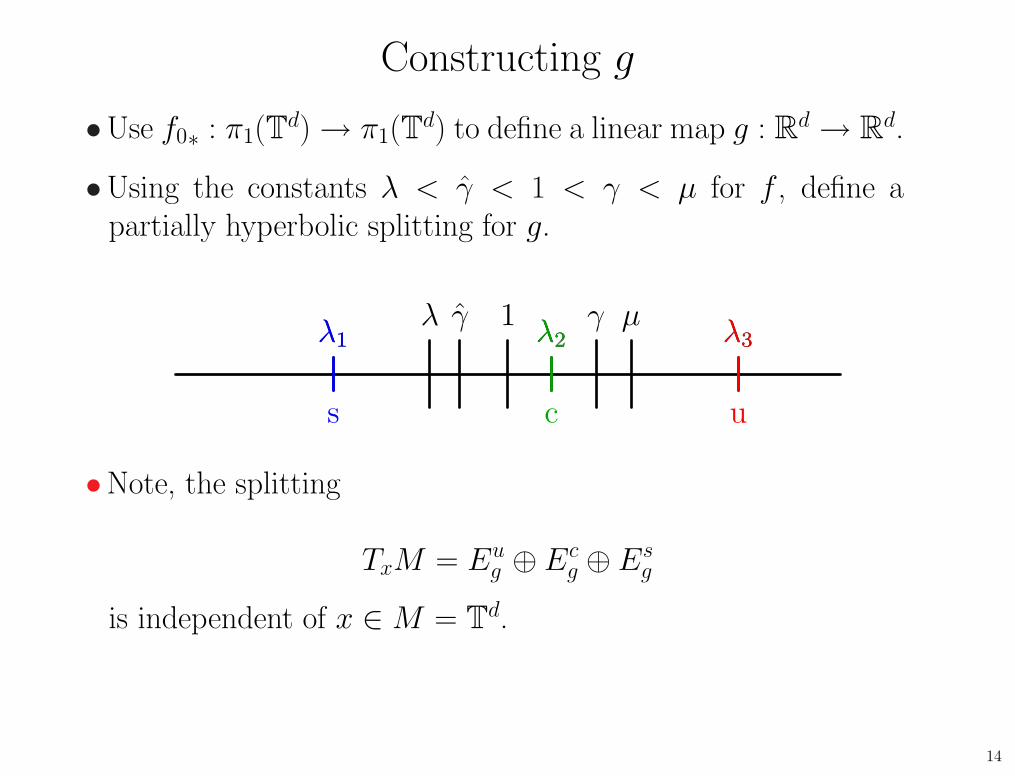
Constructing g
•Use f0∗ : π1(Td) → π1(T
d) to define a linear map g : Rd → R
d.
14

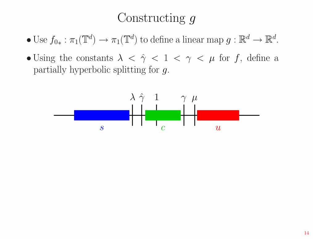
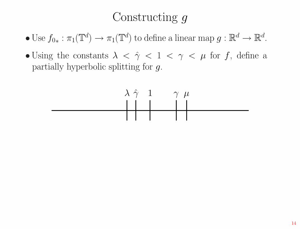
Constructing g
•Use f0∗ : π1(Td) → π1(T
d) to define a linear map g : Rd → R
d.
•Using the constants λ < γ̂ < 1 < γ < µ for f , define apartially hyperbolic splitting for g.
1
us c
14
Constructing g
•Use f0∗ : π1(Td) → π1(T
d) to define a linear map g : Rd → R
d.
•Using the constants λ < γ̂ < 1 < γ < µ for f , define apartially hyperbolic splitting for g.
1
us c
λ γ̂ γ µ
14
Constructing g
•Use f0∗ : π1(Td) → π1(T
d) to define a linear map g : Rd → R
d.
•Using the constants λ < γ̂ < 1 < γ < µ for f , define apartially hyperbolic splitting for g.
1λ γ̂ γ µ
14
Constructing g
•Use f0∗ : π1(Td) → π1(T
d) to define a linear map g : Rd → R
d.
•Using the constants λ < γ̂ < 1 < γ < µ for f , define apartially hyperbolic splitting for g.
1λ γ̂ γ µλ1
14
Constructing g
•Use f0∗ : π1(Td) → π1(T
d) to define a linear map g : Rd → R
d.
•Using the constants λ < γ̂ < 1 < γ < µ for f , define apartially hyperbolic splitting for g.
1λ γ̂ γ µλ1 λ2
14
Constructing g
•Use f0∗ : π1(Td) → π1(T
d) to define a linear map g : Rd → R
d.
•Using the constants λ < γ̂ < 1 < γ < µ for f , define apartially hyperbolic splitting for g.
1λ γ̂ γ µλ1 λ2 λ3
14
Constructing g
•Use f0∗ : π1(Td) → π1(T
d) to define a linear map g : Rd → R
d.
•Using the constants λ < γ̂ < 1 < γ < µ for f , define apartially hyperbolic splitting for g.
1λ γ̂ γ µλ1 λ2 λ3λ1
s
14

Constructing g
•Use f0∗ : π1(Td) → π1(T
d) to define a linear map g : Rd → R
d.
•Using the constants λ < γ̂ < 1 < γ < µ for f , define apartially hyperbolic splitting for g.
1λ γ̂ γ µλ1 λ2 λ3λ1
s
λ2
c
14
Constructing g
•Use f0∗ : π1(Td) → π1(T
d) to define a linear map g : Rd → R
d.
•Using the constants λ < γ̂ < 1 < γ < µ for f , define apartially hyperbolic splitting for g.
1λ γ̂ γ µλ1 λ2 λ3λ1
s
λ2
c
λ3
u
14
Constructing g
•Use f0∗ : π1(Td) → π1(T
d) to define a linear map g : Rd → R
d.
•Using the constants λ < γ̂ < 1 < γ < µ for f , define apartially hyperbolic splitting for g.
1λ γ̂ γ µλ1 λ2 λ3λ1
s
λ2
c
λ3
u
•Note, the splitting
TxM = Eug ⊕ Ec
g ⊕ Esg
is independent of x ∈ M = Td.
14
Comparing Foliations
•Compare the foliations of f to the flat, linear foliations of g.
15
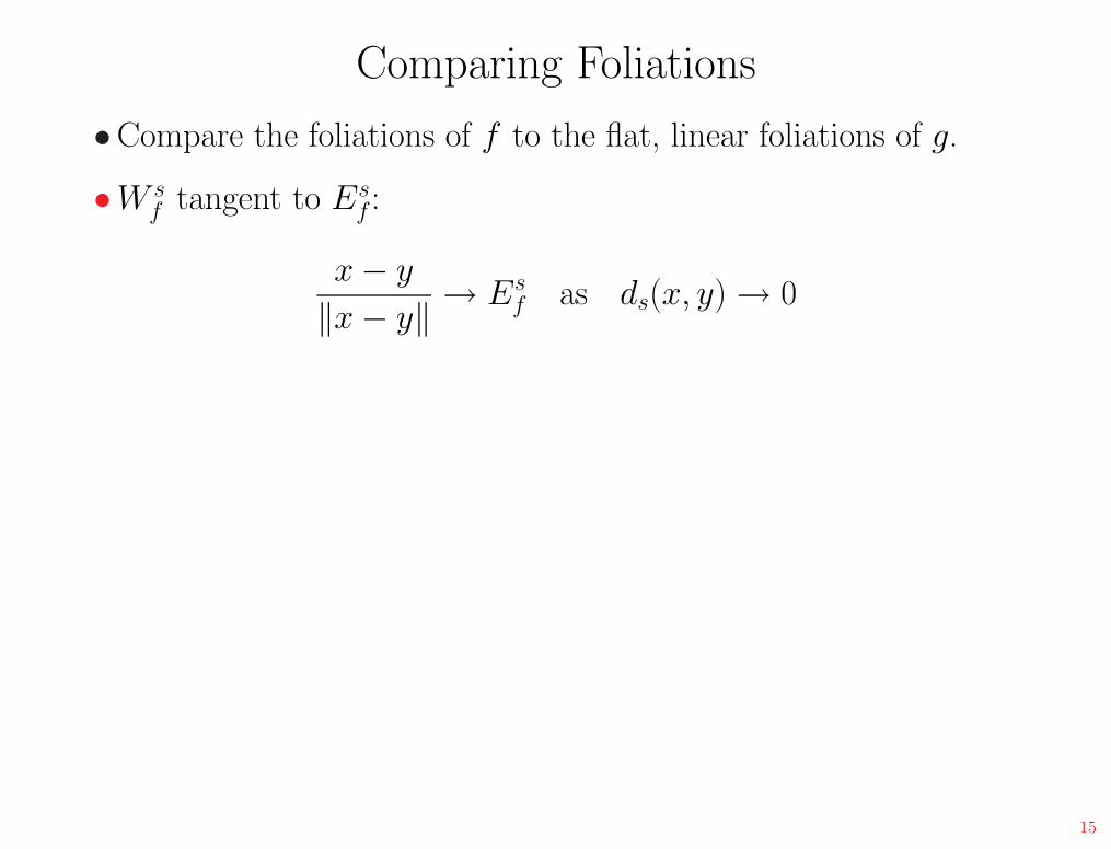
Comparing Foliations
•Compare the foliations of f to the flat, linear foliations of g.
•W sf tangent to Es
f :
x − y
‖x − y‖→ Es
f as ds(x, y) → 0
15

Comparing Foliations
•Compare the foliations of f to the flat, linear foliations of g.
•W sf tangent to Es
f :
x − y
‖x − y‖→ Es
f as ds(x, y) → 0
•What if ds(x, y) → ∞?
15
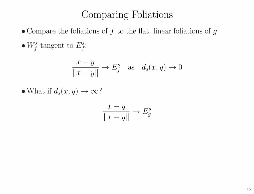
Comparing Foliations
•Compare the foliations of f to the flat, linear foliations of g.
•W sf tangent to Es
f :
x − y
‖x − y‖→ Es
f as ds(x, y) → 0
•What if ds(x, y) → ∞?
x − y
‖x − y‖→ Es
g
15
Three Scales
Euf (x)
Esf (x)
Ecf (x)
xW u
f (x)
W sf (x)
W cf (x)
16
Three Scales
Euf (x)
Esf (x)
Ecf (x)
xW u
f (x)
W sf (x)
W cf (x)
16
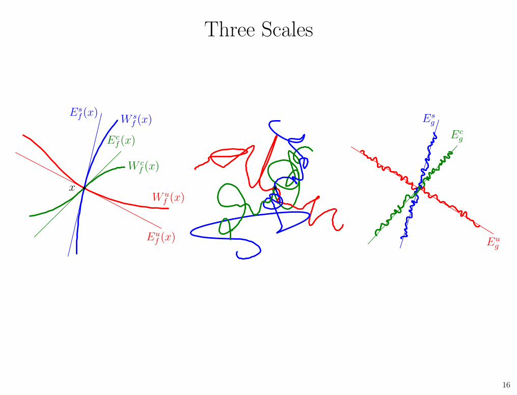
Three Scales
Euf (x)
Esf (x)
Ecf (x)
xW u
f (x)
W sf (x)
W cf (x)
Eug
Esg
Ecg
16
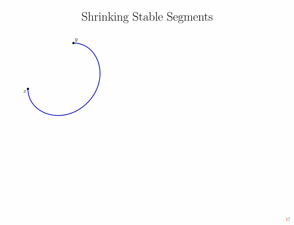
Shrinking Stable Segments
x
y
17
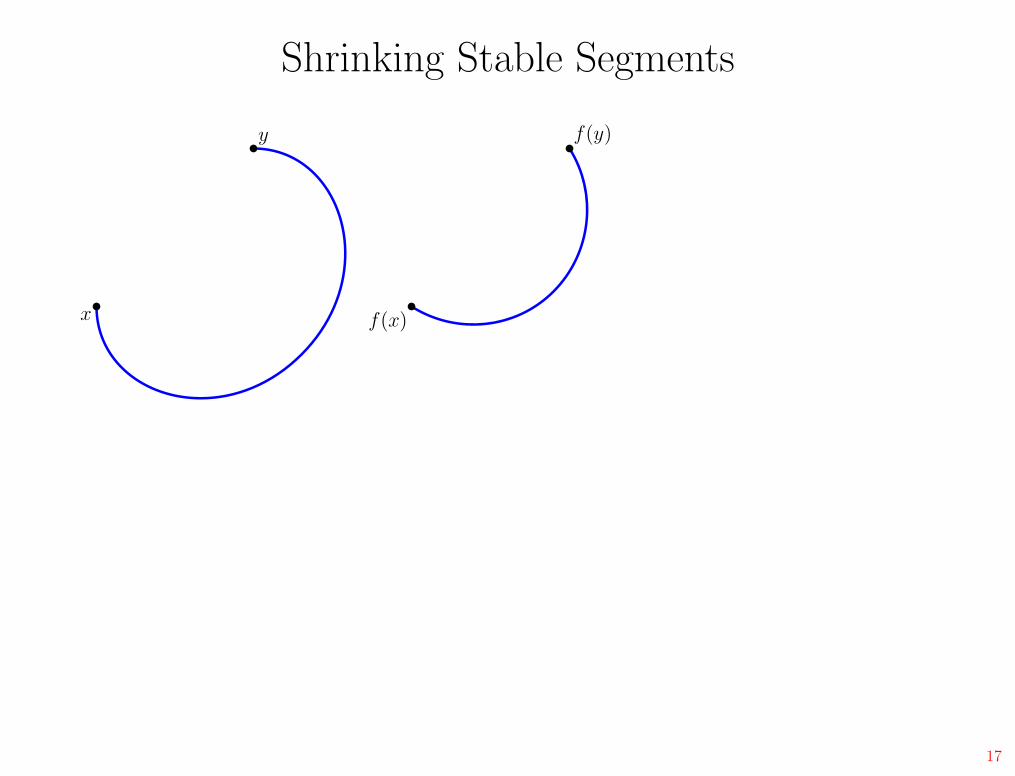
Shrinking Stable Segments
x
y
f(x)
f(y)
17
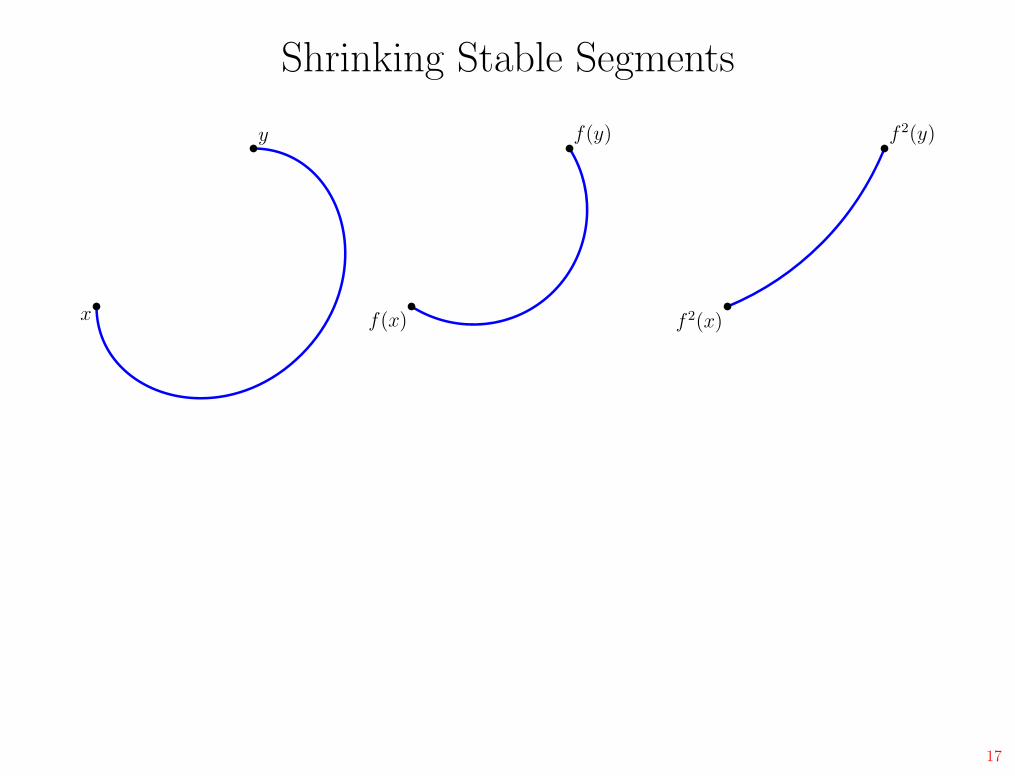
Shrinking Stable Segments
x
y
f(x)
f(y)
f 2(x)
f 2(y)
17
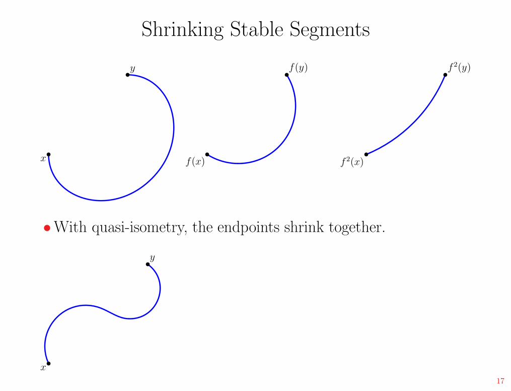
Shrinking Stable Segments
x
y
f(x)
f(y)
f 2(x)
f 2(y)
•With quasi-isometry, the endpoints shrink together.
x
y
17
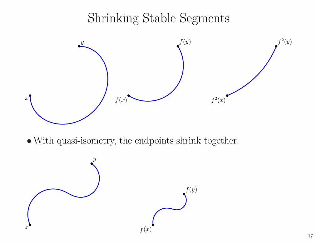
Shrinking Stable Segments
x
y
f(x)
f(y)
f 2(x)
f 2(y)
•With quasi-isometry, the endpoints shrink together.
x
y
f(x)
f(y)
17

Shrinking Stable Segments
x
y
f(x)
f(y)
f 2(x)
f 2(y)
•With quasi-isometry, the endpoints shrink together.
x
y
f(x)
f(y)
f 2(x)
f 2(y)
17

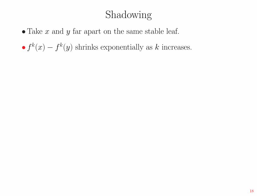
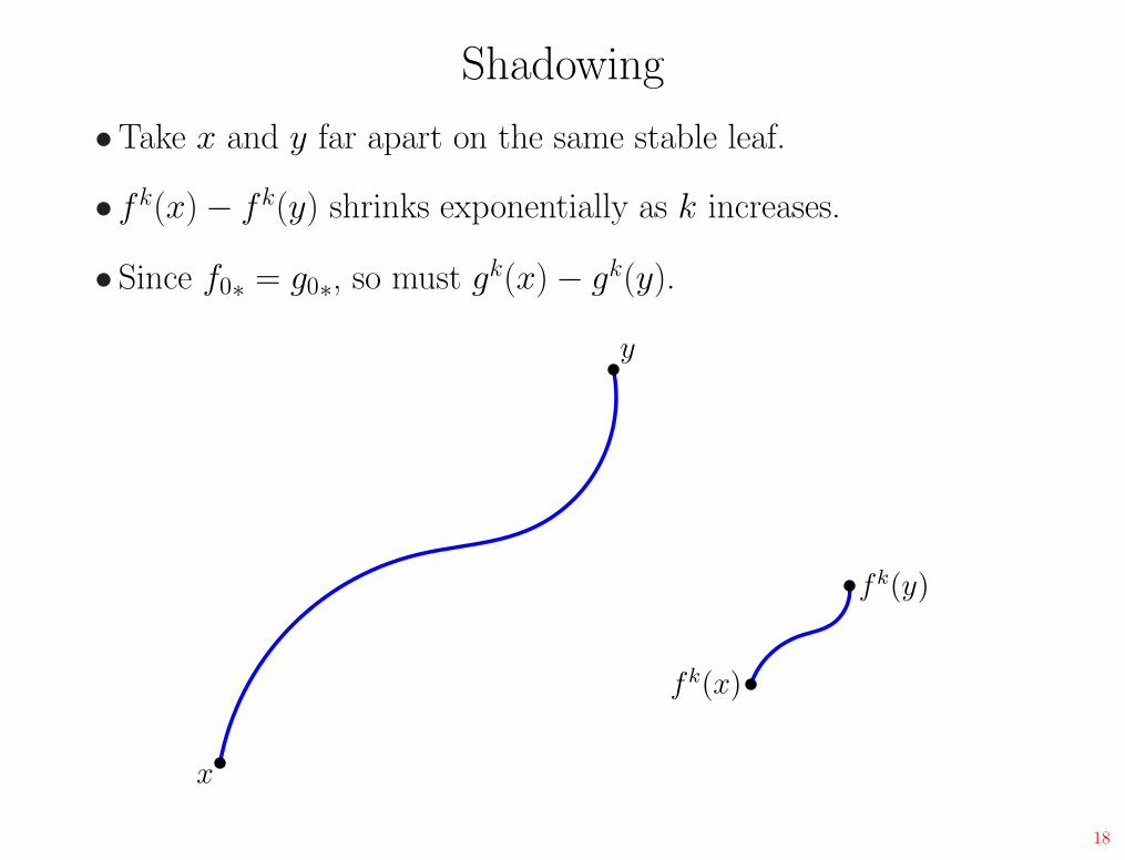
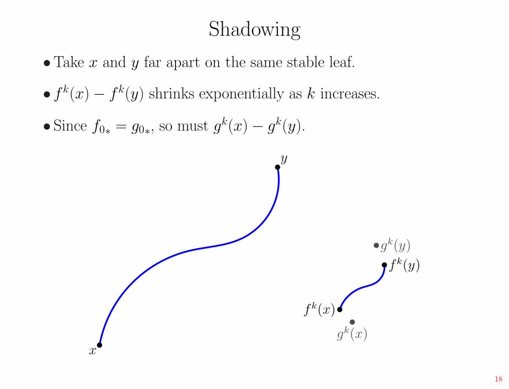
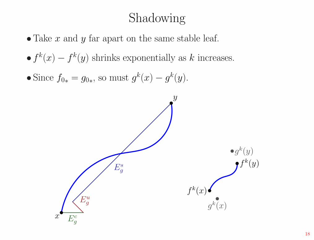
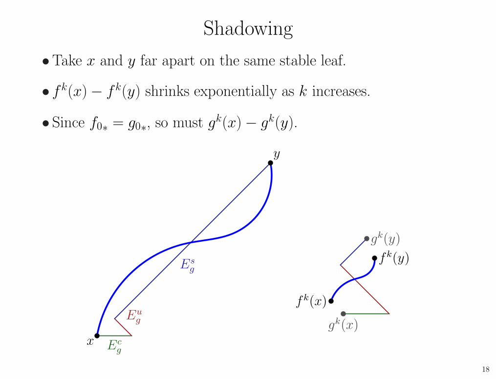
Shadowing
•Take x and y far apart on the same stable leaf.
18
Shadowing
•Take x and y far apart on the same stable leaf.
• fk(x) − fk(y) shrinks exponentially as k increases.
18

Shadowing
•Take x and y far apart on the same stable leaf.
• fk(x) − fk(y) shrinks exponentially as k increases.
• Since f0∗ = g0∗, so must gk(x) − gk(y).
18

Shadowing
•Take x and y far apart on the same stable leaf.
• fk(x) − fk(y) shrinks exponentially as k increases.
• Since f0∗ = g0∗, so must gk(x) − gk(y).
x
y
18
Shadowing
•Take x and y far apart on the same stable leaf.
• fk(x) − fk(y) shrinks exponentially as k increases.
• Since f0∗ = g0∗, so must gk(x) − gk(y).
x
y
fk(x)
fk(y)
18
Shadowing
•Take x and y far apart on the same stable leaf.
• fk(x) − fk(y) shrinks exponentially as k increases.
• Since f0∗ = g0∗, so must gk(x) − gk(y).
x
y
fk(x)
fk(y)
gk(x)
gk(y)
18
Shadowing
•Take x and y far apart on the same stable leaf.
• fk(x) − fk(y) shrinks exponentially as k increases.
• Since f0∗ = g0∗, so must gk(x) − gk(y).
Ecg
Eug
Esg
x
y
fk(x)
fk(y)
gk(x)
gk(y)
18
Shadowing
•Take x and y far apart on the same stable leaf.
• fk(x) − fk(y) shrinks exponentially as k increases.
• Since f0∗ = g0∗, so must gk(x) − gk(y).
Ecg
Eug
Esg
x
y
fk(x)
fk(y)
gk(x)
gk(y)
18
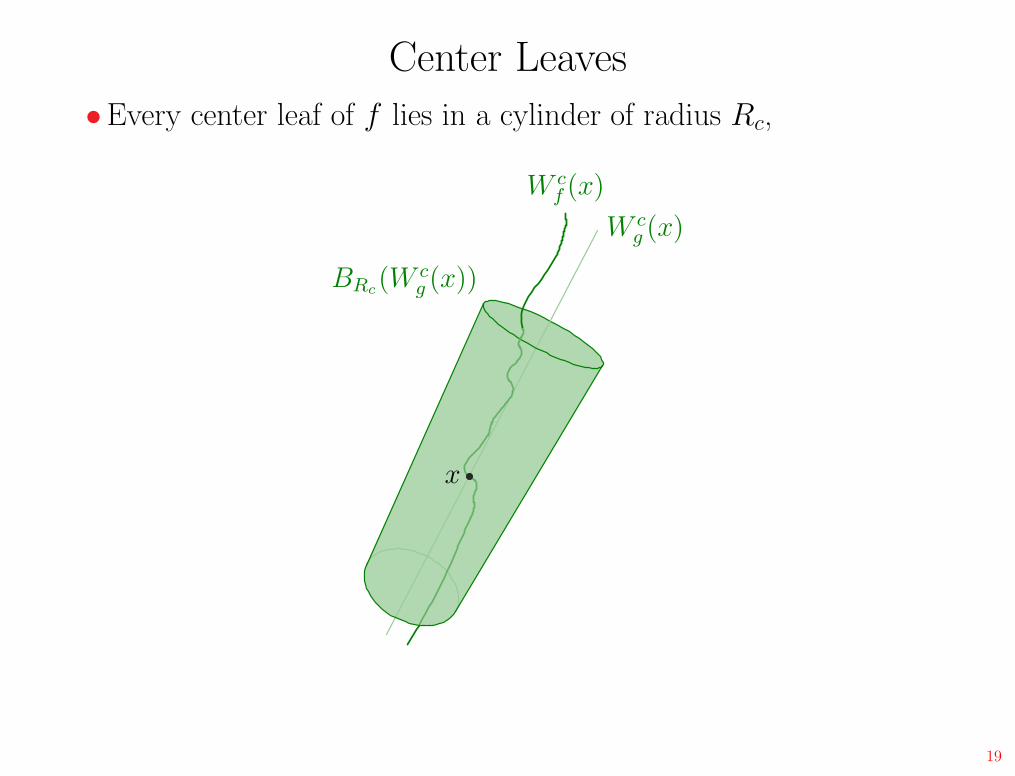
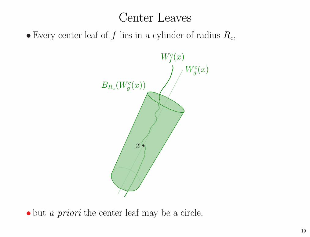
Center Leaves
•Every center leaf of f lies in a cylinder of radius Rc,
x
BRc(W c
g (x))
Wcf (x)
Wcg (x)
19
Center Leaves
•Every center leaf of f lies in a cylinder of radius Rc,
x
BRc(W c
g (x))
Wcf (x)
Wcg (x)
• but a priori the center leaf may be a circle.
19
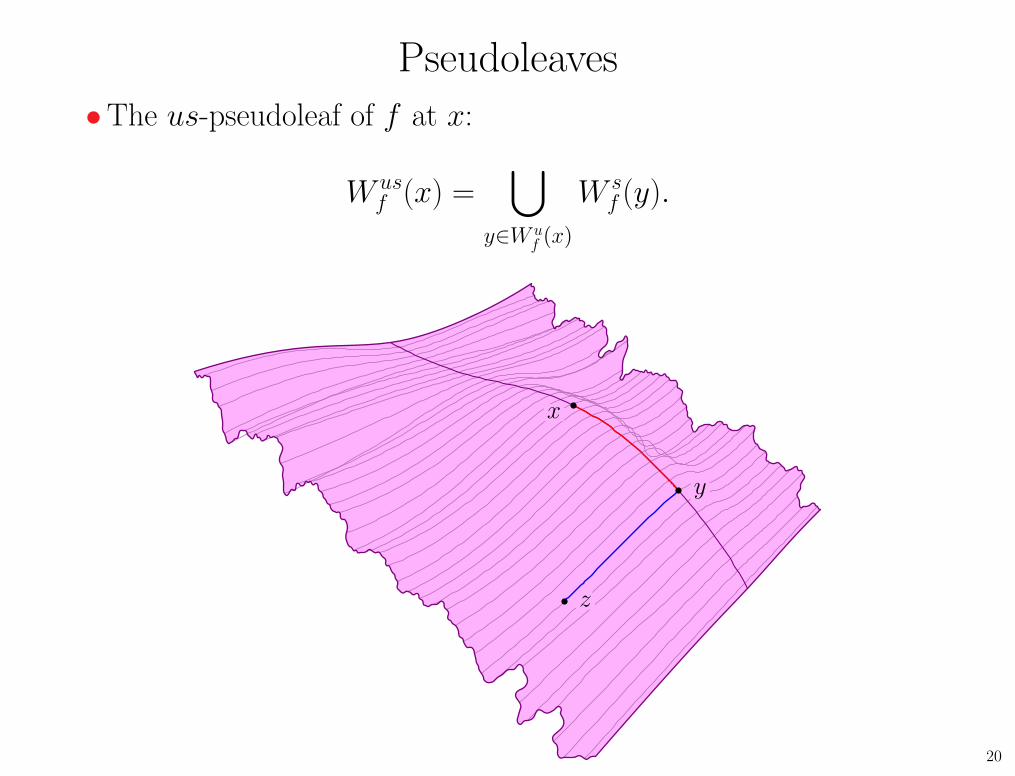
Pseudoleaves
•The us-pseudoleaf of f at x:
W usf (x) =
⋃
y∈W uf (x)
W sf (y).
x
y
z
20
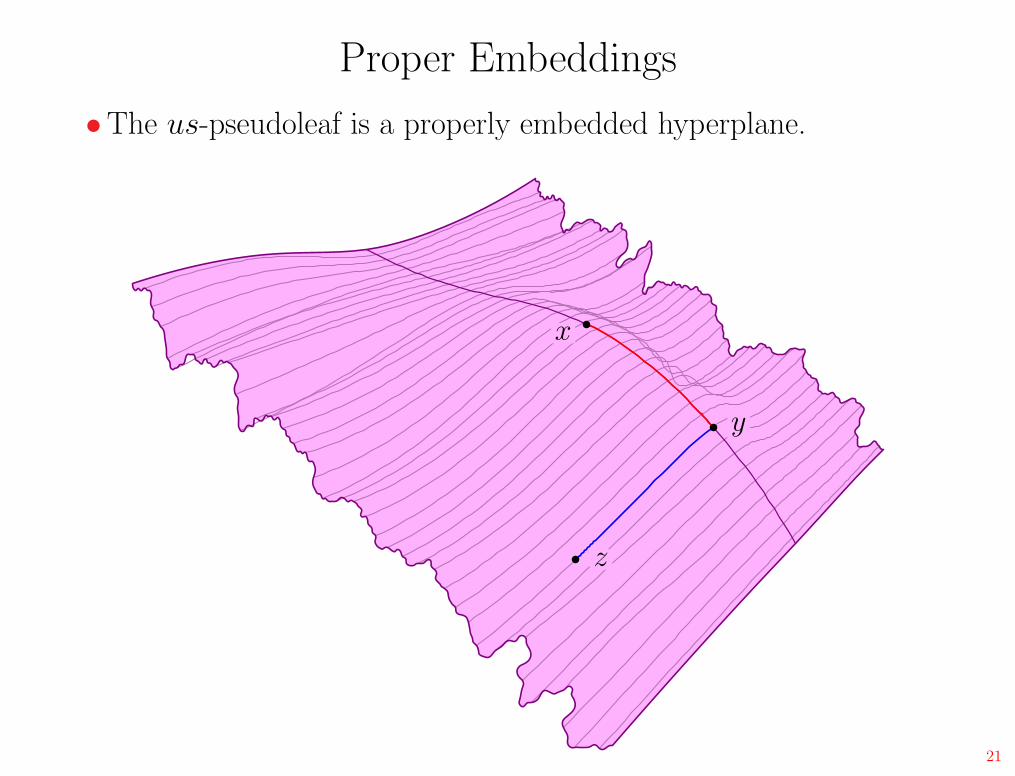
Proper Embeddings
•The us-pseudoleaf is a properly embedded hyperplane.
x
y
z
21
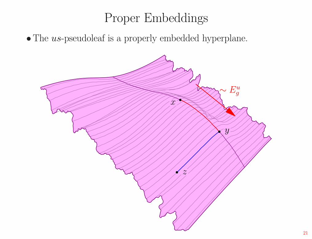
Proper Embeddings
•The us-pseudoleaf is a properly embedded hyperplane.
x
y
z
∼ Eug
21

Proper Embeddings
•The us-pseudoleaf is a properly embedded hyperplane.
x
y
z
∼ Eug
∼ Esg
21
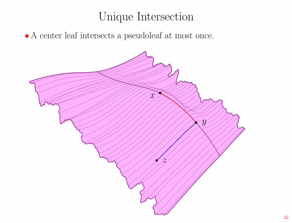
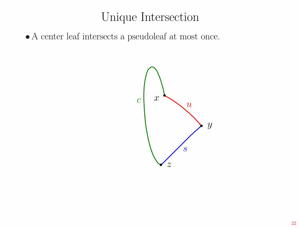
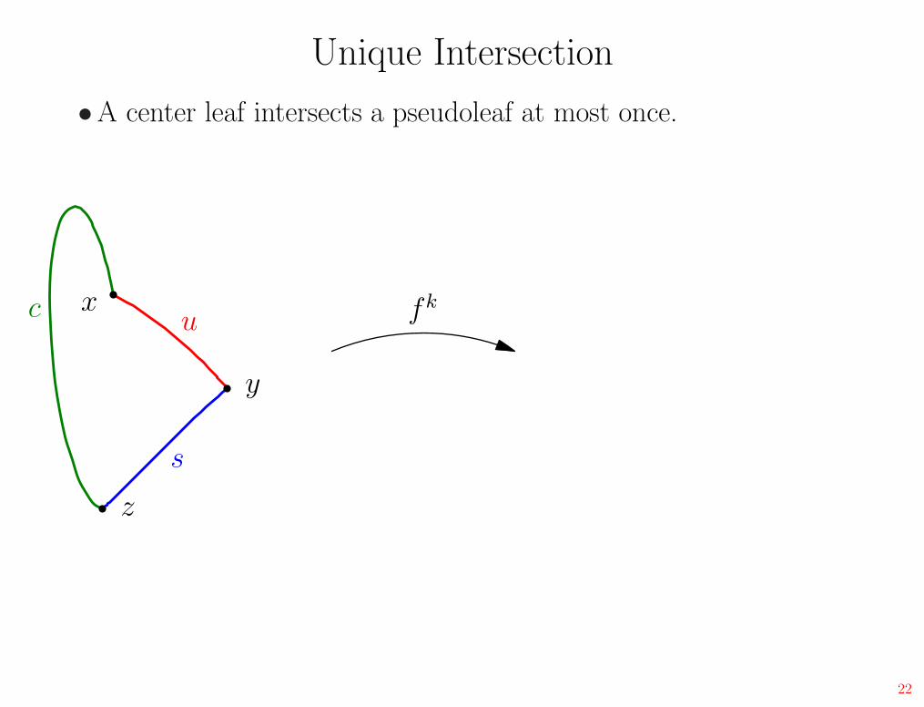
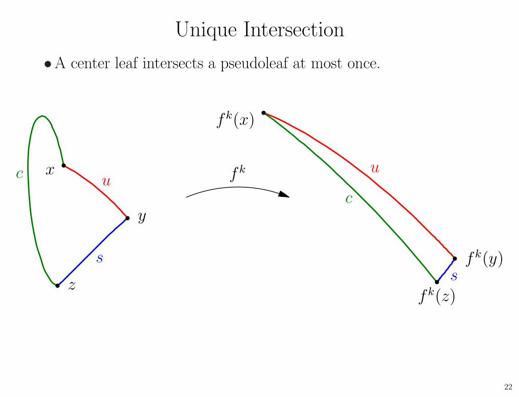
Unique Intersection
•A center leaf intersects a pseudoleaf at most once.
x
y
z
22

Unique Intersection
•A center leaf intersects a pseudoleaf at most once.
x
y
z
22
Unique Intersection
•A center leaf intersects a pseudoleaf at most once.
s
uc x
y
z
22
Unique Intersection
•A center leaf intersects a pseudoleaf at most once.
s
uc x
y
z
fk
22
Unique Intersection
•A center leaf intersects a pseudoleaf at most once.
s
uc x
y
z
fk
s
u
c
fk(x)
fk(y)
fk(z)
22
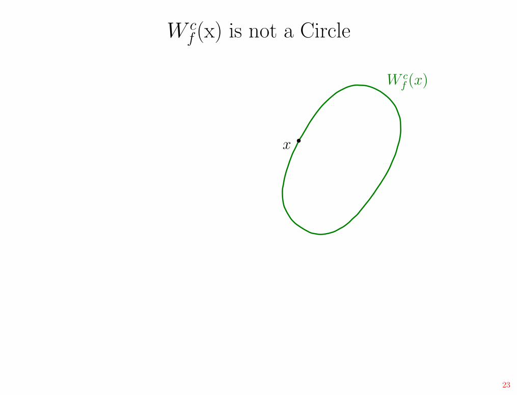
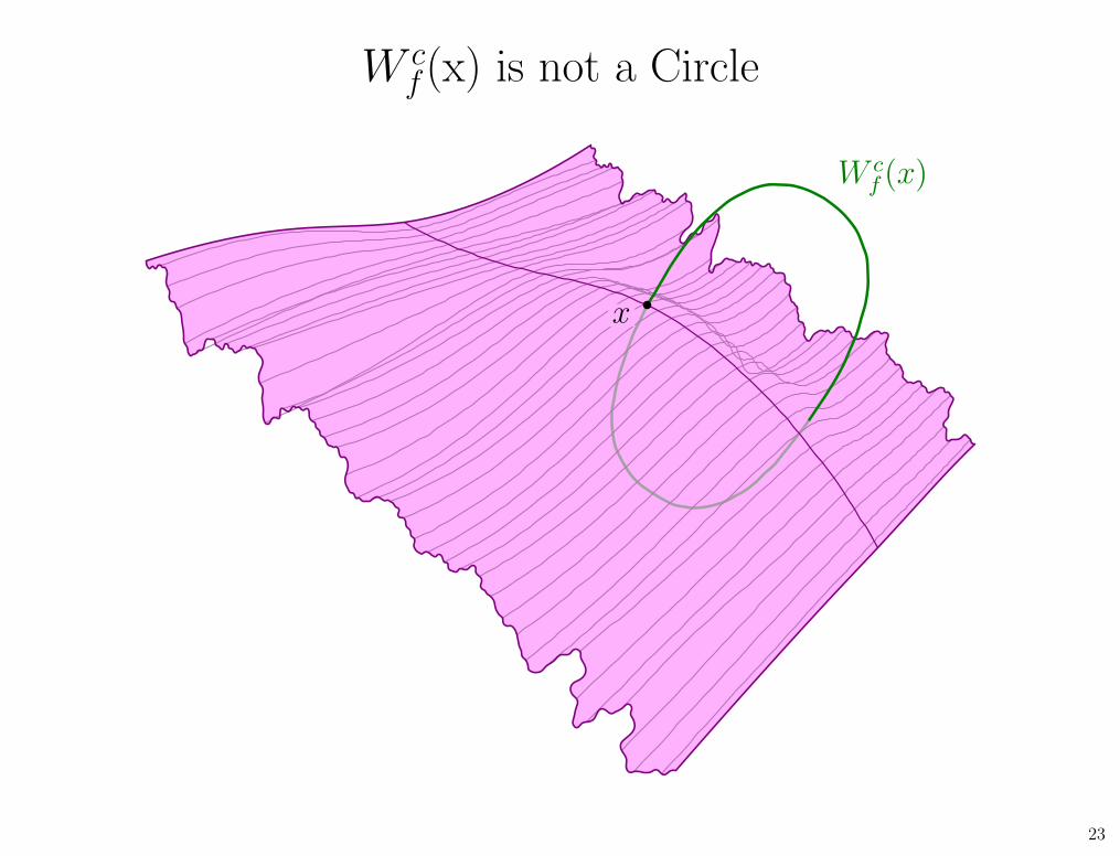
W cf (x) is not a Circle
W cf (x)
x
23
W cf (x) is not a Circle
W cf (x)
x
23
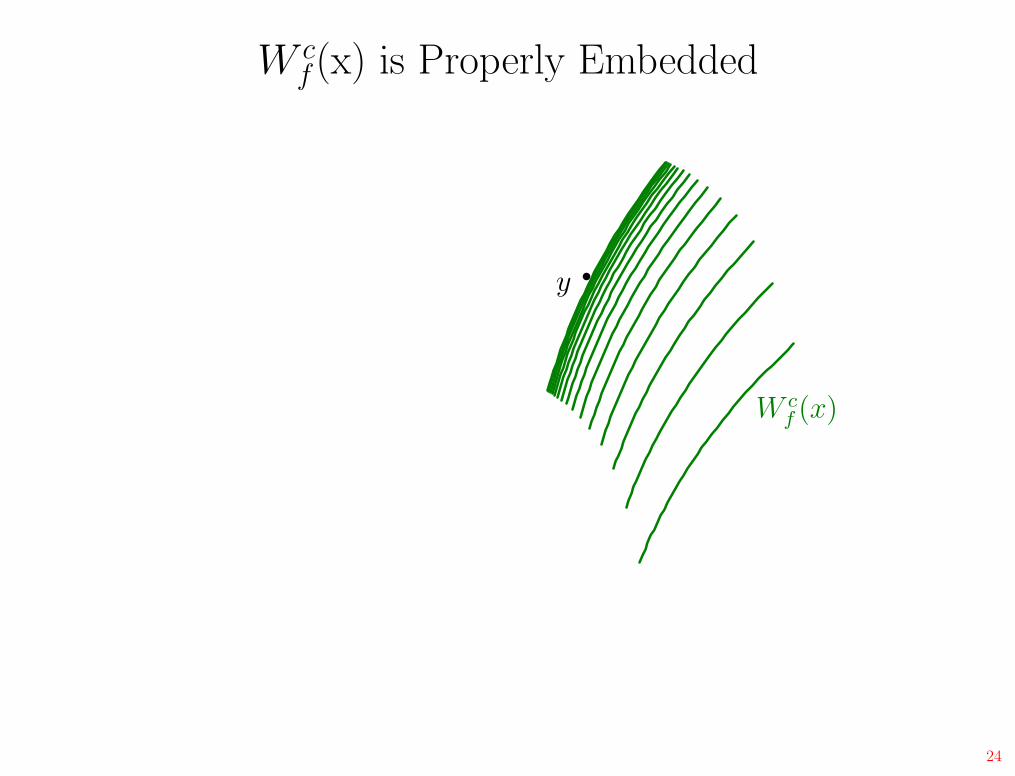
W cf (x) is Properly Embedded
W cf (x)
y
24
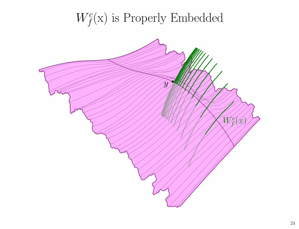
W cf (x) is Properly Embedded
y
W cf (x)
24

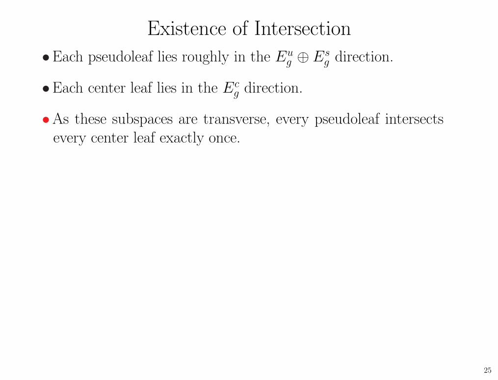
Existence of Intersection
•Each pseudoleaf lies roughly in the Eug ⊕ Es
g direction.
25
Existence of Intersection
•Each pseudoleaf lies roughly in the Eug ⊕ Es
g direction.
•Each center leaf lies in the Ecg direction.
25
Existence of Intersection
•Each pseudoleaf lies roughly in the Eug ⊕ Es
g direction.
•Each center leaf lies in the Ecg direction.
•As these subspaces are transverse, every pseudoleaf intersectsevery center leaf exactly once.
25

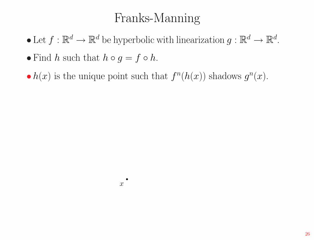
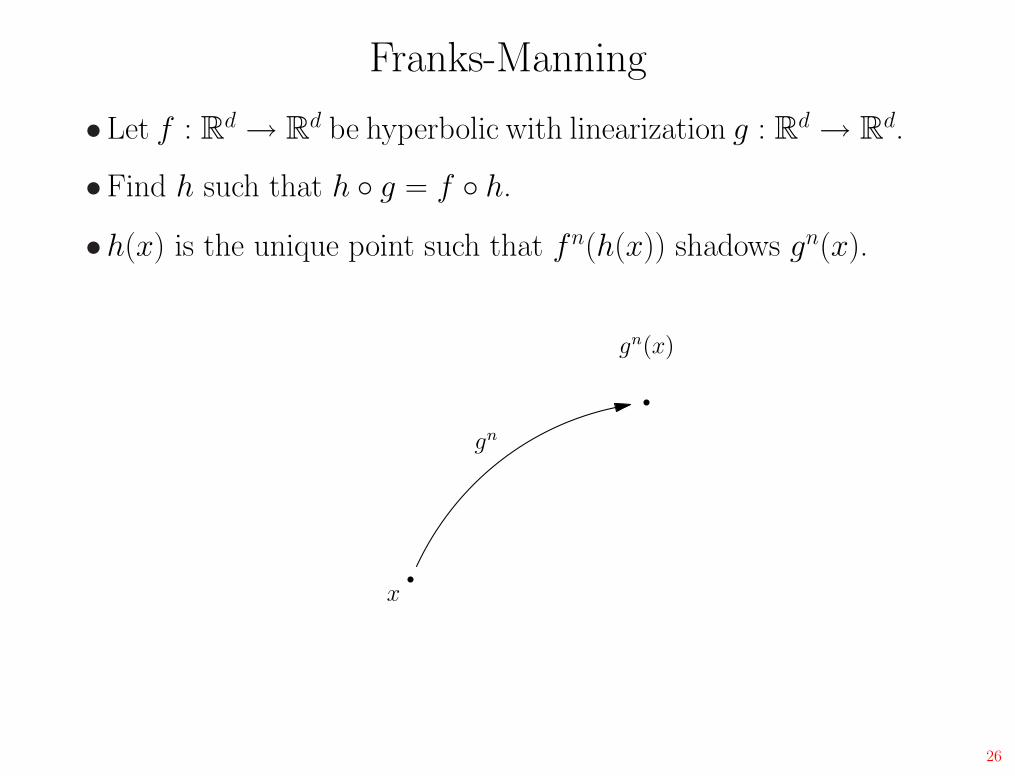
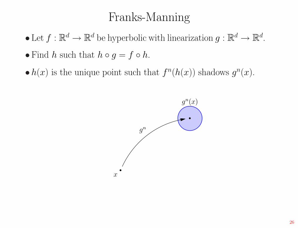
Franks-Manning
•Let f : Rd → R
d be hyperbolic with linearization g : Rd → R
d.
26
Franks-Manning
•Let f : Rd → R
d be hyperbolic with linearization g : Rd → R
d.
•Find h such that h ◦ g = f ◦ h.
26
Franks-Manning
•Let f : Rd → R
d be hyperbolic with linearization g : Rd → R
d.
•Find h such that h ◦ g = f ◦ h.
•h(x) is the unique point such that fn(h(x)) shadows gn(x).
x
26
Franks-Manning
•Let f : Rd → R
d be hyperbolic with linearization g : Rd → R
d.
•Find h such that h ◦ g = f ◦ h.
•h(x) is the unique point such that fn(h(x)) shadows gn(x).
x
gn(x)
gn
26
Franks-Manning
•Let f : Rd → R
d be hyperbolic with linearization g : Rd → R
d.
•Find h such that h ◦ g = f ◦ h.
•h(x) is the unique point such that fn(h(x)) shadows gn(x).
x
gn(x)
gn
26
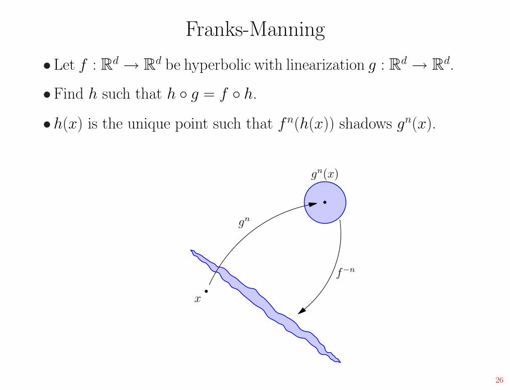
Franks-Manning
•Let f : Rd → R
d be hyperbolic with linearization g : Rd → R
d.
•Find h such that h ◦ g = f ◦ h.
•h(x) is the unique point such that fn(h(x)) shadows gn(x).
x
gn(x)
gn
f−n
26
Franks-Manning
•Let f : Rd → R
d be hyperbolic with linearization g : Rd → R
d.
•Find h such that h ◦ g = f ◦ h.
•h(x) is the unique point such that fn(h(x)) shadows gn(x).
x
gn(x)
gn
f−n
g−n(x)
g−n
26

Franks-Manning
•Let f : Rd → R
d be hyperbolic with linearization g : Rd → R
d.
•Find h such that h ◦ g = f ◦ h.
•h(x) is the unique point such that fn(h(x)) shadows gn(x).
x
gn(x)
gn
f−n
g−n(x)
g−n
26
Franks-Manning
•Let f : Rd → R
d be hyperbolic with linearization g : Rd → R
d.
•Find h such that h ◦ g = f ◦ h.
•h(x) is the unique point such that fn(h(x)) shadows gn(x).
x
gn(x)
gn
f−n
g−n(x)
g−n
fn
26
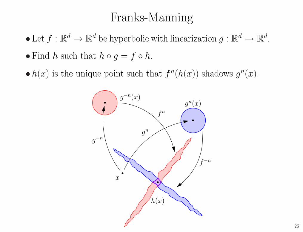
Franks-Manning
•Let f : Rd → R
d be hyperbolic with linearization g : Rd → R
d.
•Find h such that h ◦ g = f ◦ h.
•h(x) is the unique point such that fn(h(x)) shadows gn(x).
x
gn(x)
gn
f−n
g−n(x)
g−n
fn
h(x)
26
Franks-Manning Reloaded
L
27

Franks-Manning Reloaded
L
gn
gn(L)
27

Franks-Manning Reloaded
L
gn
gn(L)
27
Franks-Manning Reloaded
L
gn
gn(L)
f−n
27
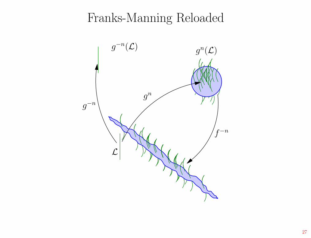
Franks-Manning Reloaded
L
gn
gn(L)
f−n
g−n
g−n(L)
27
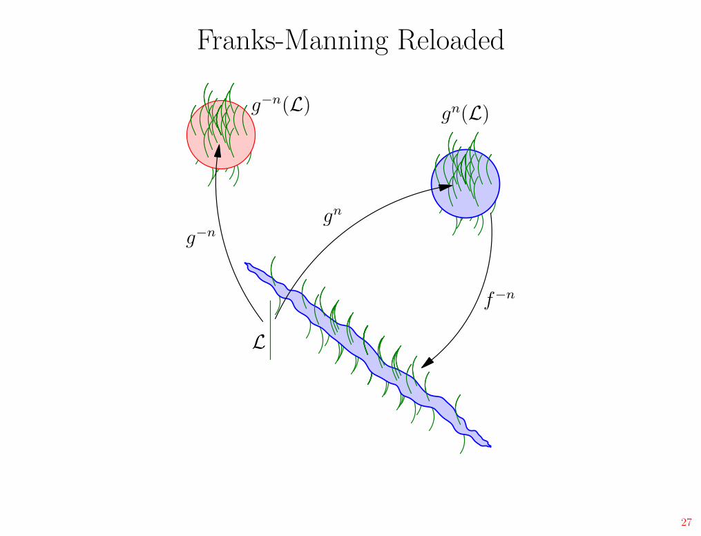
Franks-Manning Reloaded
L
gn
gn(L)
f−n
g−n
g−n(L)
27
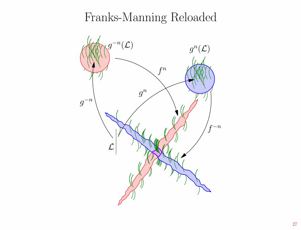
Franks-Manning Reloaded
L
gn
gn(L)
f−n
g−n
g−n(L)
fn
27
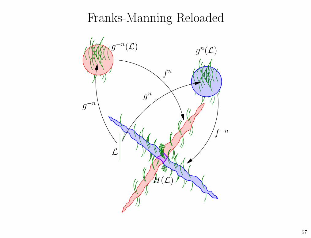
Franks-Manning Reloaded
L
gn
gn(L)
f−n
g−n
g−n(L)
fn
H(L)
27
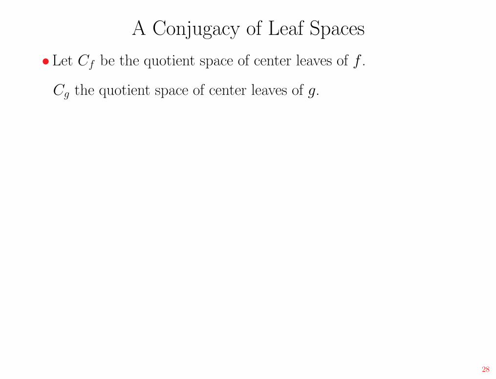
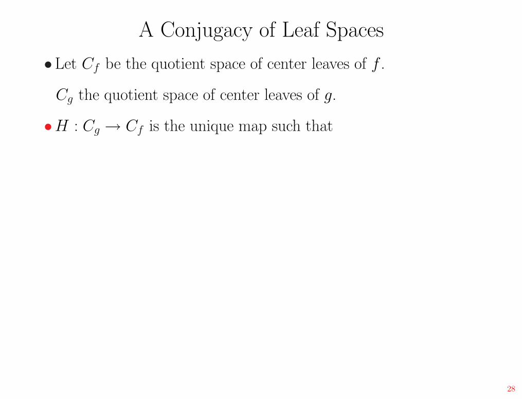
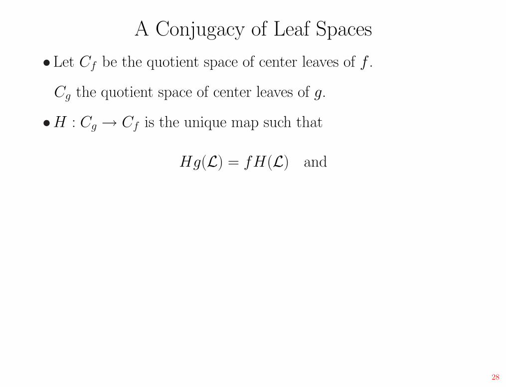
A Conjugacy of Leaf Spaces
•Let Cf be the quotient space of center leaves of f .
Cg the quotient space of center leaves of g.
28
A Conjugacy of Leaf Spaces
•Let Cf be the quotient space of center leaves of f .
Cg the quotient space of center leaves of g.
•H : Cg → Cf is the unique map such that
28
A Conjugacy of Leaf Spaces
•Let Cf be the quotient space of center leaves of f .
Cg the quotient space of center leaves of g.
•H : Cg → Cf is the unique map such that
Hg(L) = fH(L) and
28
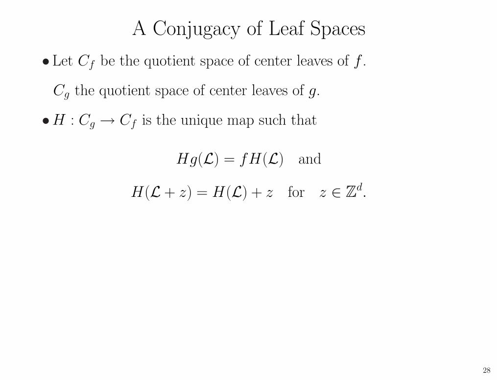
A Conjugacy of Leaf Spaces
•Let Cf be the quotient space of center leaves of f .
Cg the quotient space of center leaves of g.
•H : Cg → Cf is the unique map such that
Hg(L) = fH(L) and
H(L + z) = H(L) + z for z ∈ Zd.
28
Characterizing f
•We know the topology of the leaves, and the directions in whichthey lie.
29
Characterizing f
•We know the topology of the leaves, and the directions in whichthey lie.
•We know how the leaves intersect.
29
Characterizing f
•We know the topology of the leaves, and the directions in whichthey lie.
•We know how the leaves intersect.
•H : Cg → Cf shows that f acts on center leaves as a hyperboliclinear map.
29
Characterizing f
•We know the topology of the leaves, and the directions in whichthey lie.
•We know how the leaves intersect.
•H : Cg → Cf shows that f acts on center leaves as a hyperboliclinear map.
•Now construct a leaf conjugacy h0 : Rd → R
d from H .
29

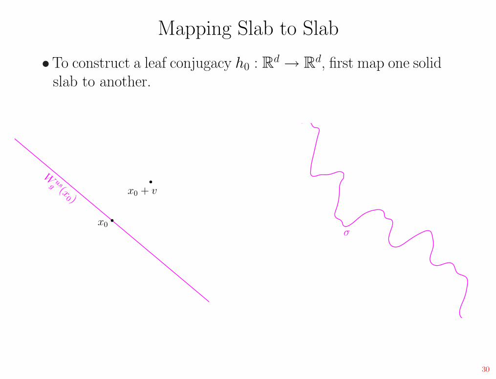
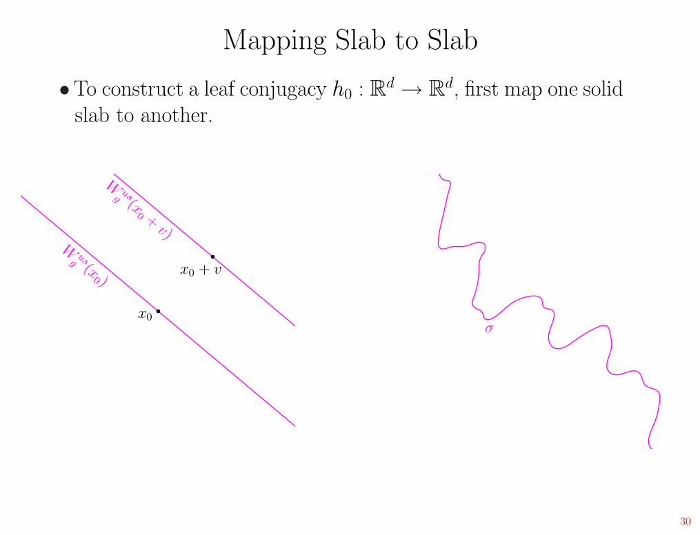
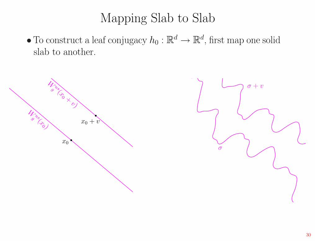
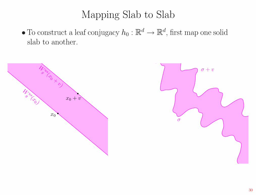
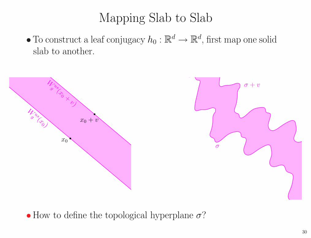
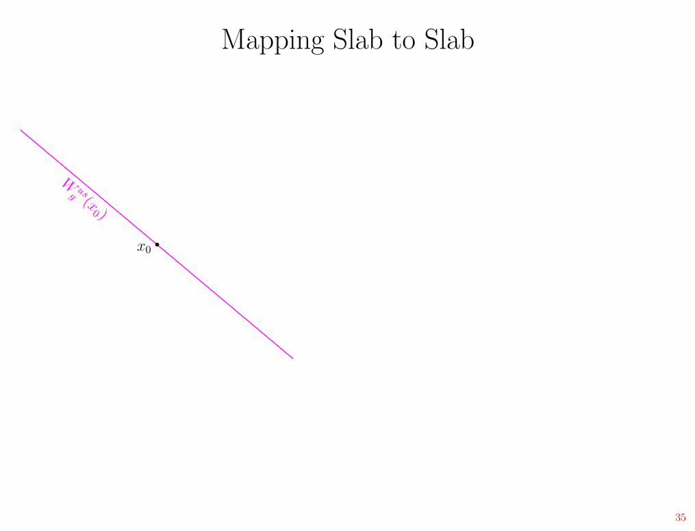
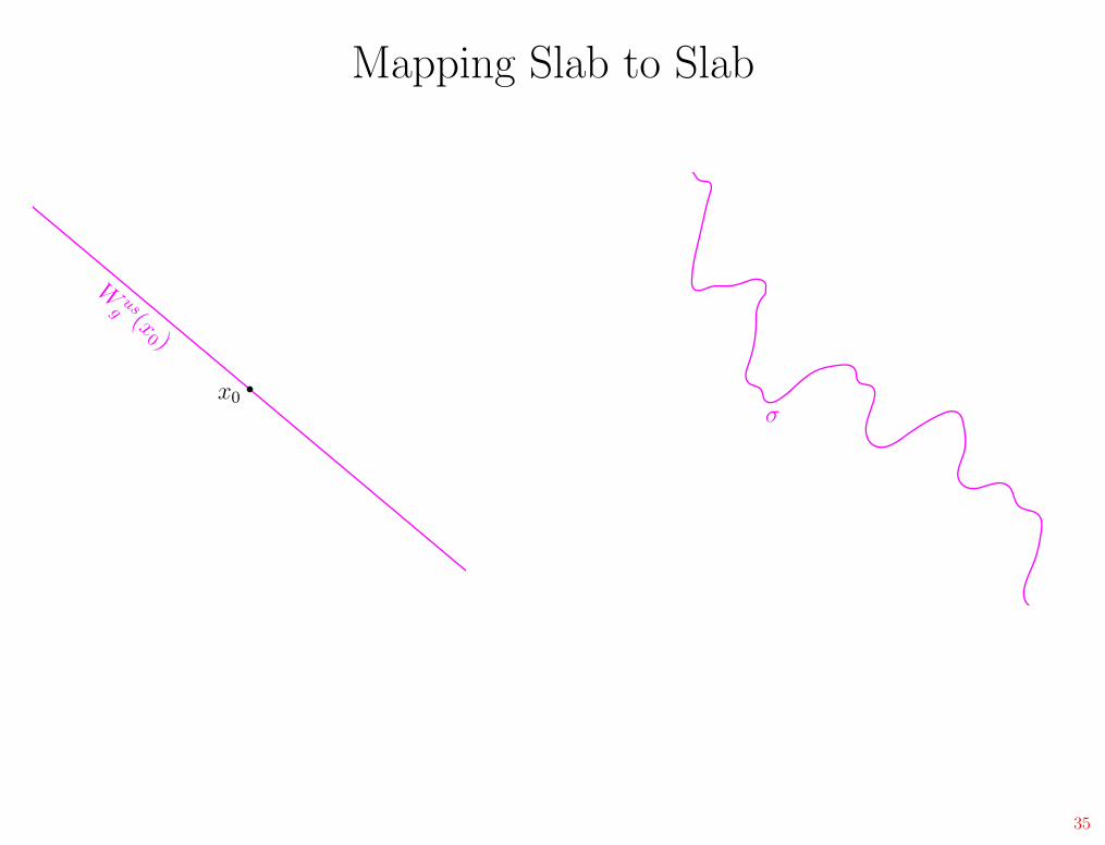
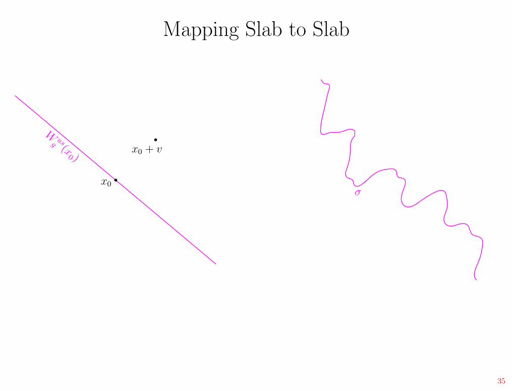
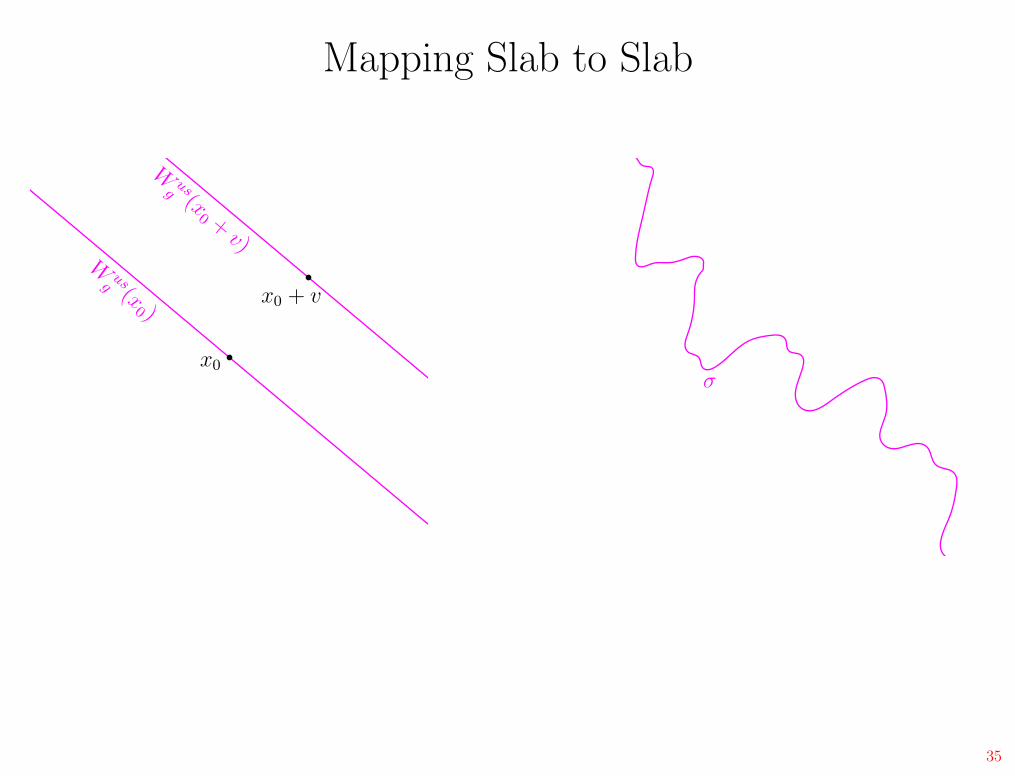
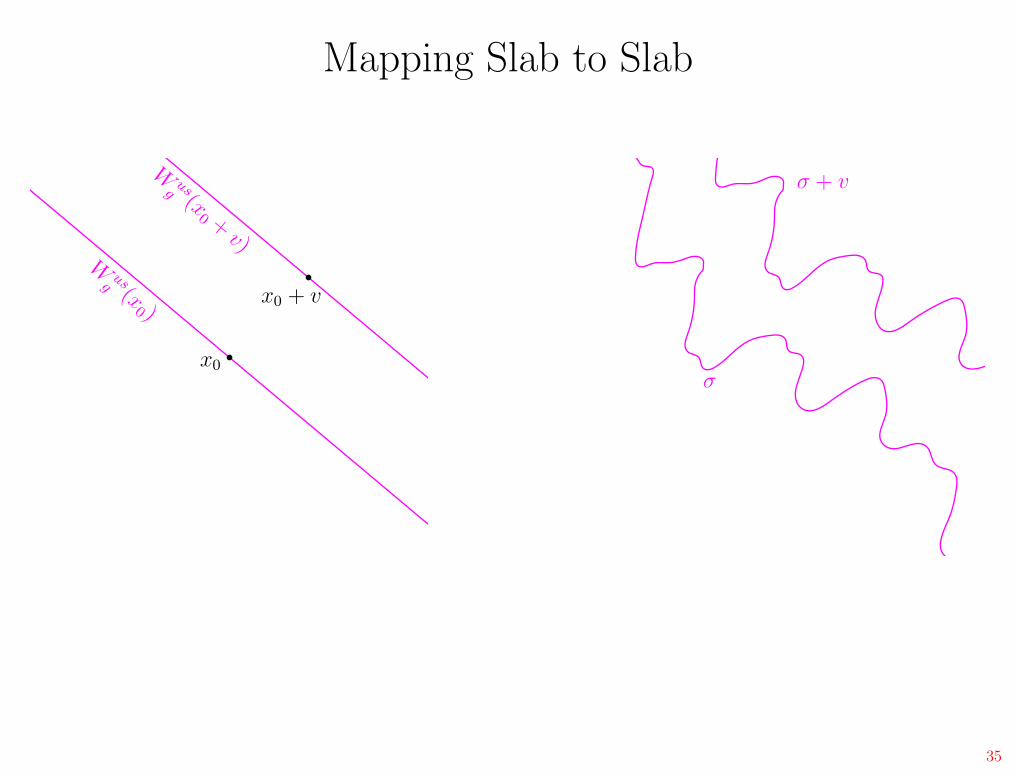
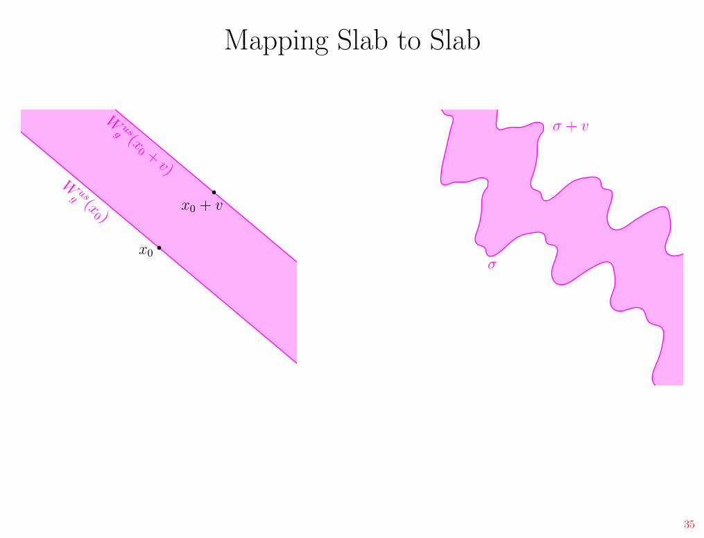
Mapping Slab to Slab
•To construct a leaf conjugacy h0 : Rd → R
d, first map one solidslab to another.
x0
30

Mapping Slab to Slab
•To construct a leaf conjugacy h0 : Rd → R
d, first map one solidslab to another.
x0
Wusg (x
0 )
30
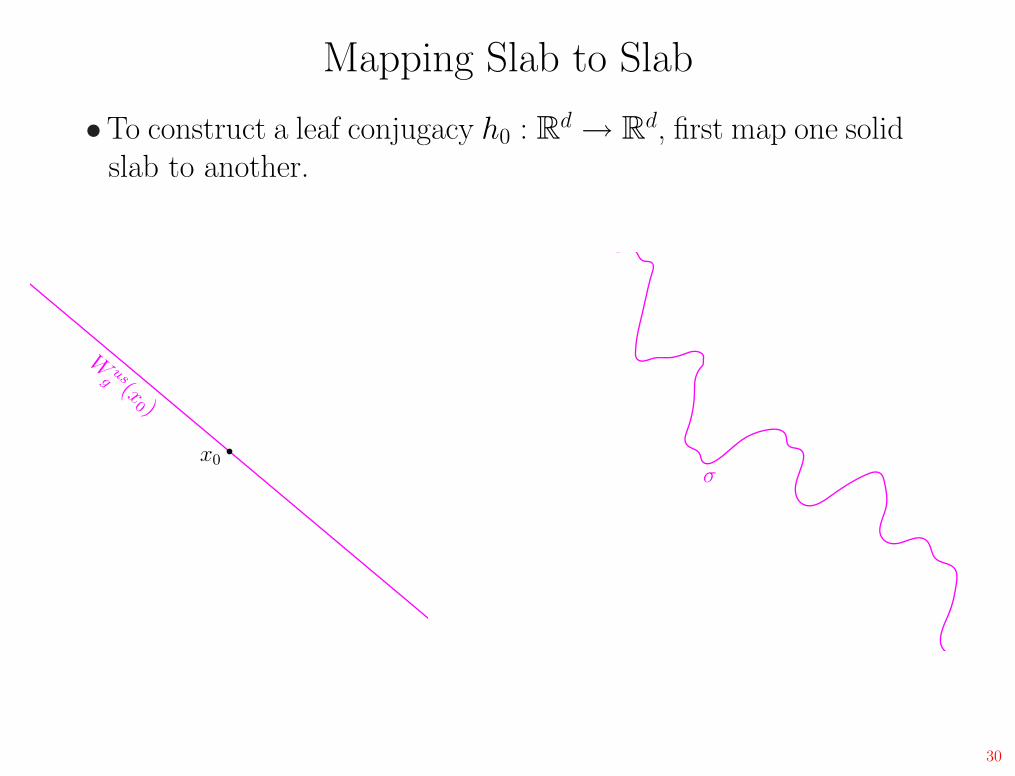
Mapping Slab to Slab
•To construct a leaf conjugacy h0 : Rd → R
d, first map one solidslab to another.
x0
Wusg (x
0 )
σ
30
Mapping Slab to Slab
•To construct a leaf conjugacy h0 : Rd → R
d, first map one solidslab to another.
x0
Wusg (x
0 )x0 + v
σ
30
Mapping Slab to Slab
•To construct a leaf conjugacy h0 : Rd → R
d, first map one solidslab to another.
x0
Wusg (x
0 )x0 + v
Wusg (x
0 +v)
σ
30
Mapping Slab to Slab
•To construct a leaf conjugacy h0 : Rd → R
d, first map one solidslab to another.
x0
Wusg (x
0 )x0 + v
Wusg (x
0 +v)
σ
σ + v
30
Mapping Slab to Slab
•To construct a leaf conjugacy h0 : Rd → R
d, first map one solidslab to another.
x0
Wusg (x
0 )x0 + v
Wusg (x
0 +v)
σ
σ + v
30
Mapping Slab to Slab
•To construct a leaf conjugacy h0 : Rd → R
d, first map one solidslab to another.
x0
Wusg (x
0 )x0 + v
Wusg (x
0 +v)
σ
σ + v
•How to define the topological hyperplane σ?
30
Sections
Definition. A section is a continuous map σ : Cf → Rd such
that
31
Sections
Definition. A section is a continuous map σ : Cf → Rd such
that
σ(L) is on the leaf L for L ∈ Cf .
31
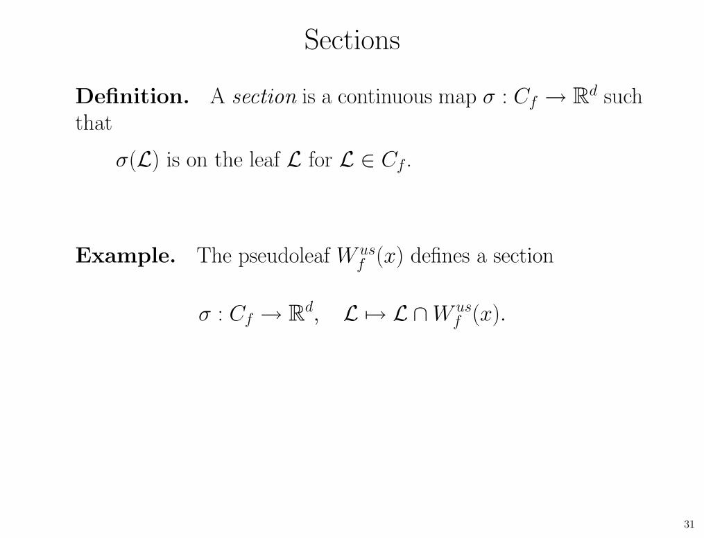
Sections
Definition. A section is a continuous map σ : Cf → Rd such
that
σ(L) is on the leaf L for L ∈ Cf .
Example. The pseudoleaf W usf (x) defines a section
σ : Cf → Rd, L 7→ L ∩ W us
f (x).
31
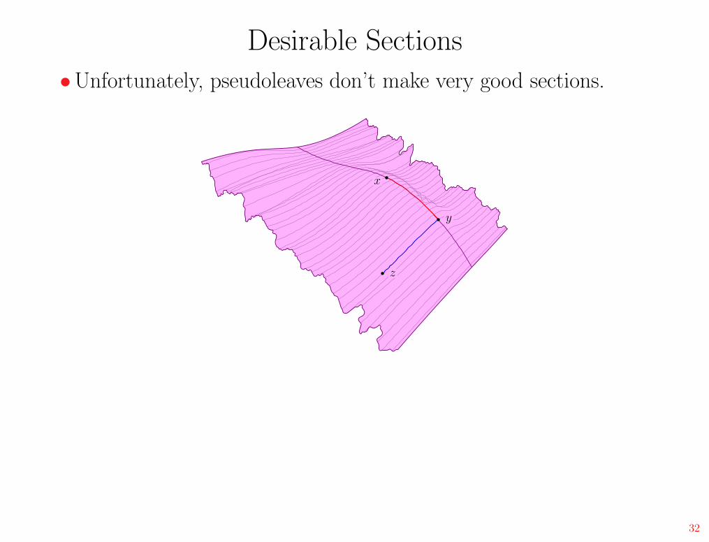
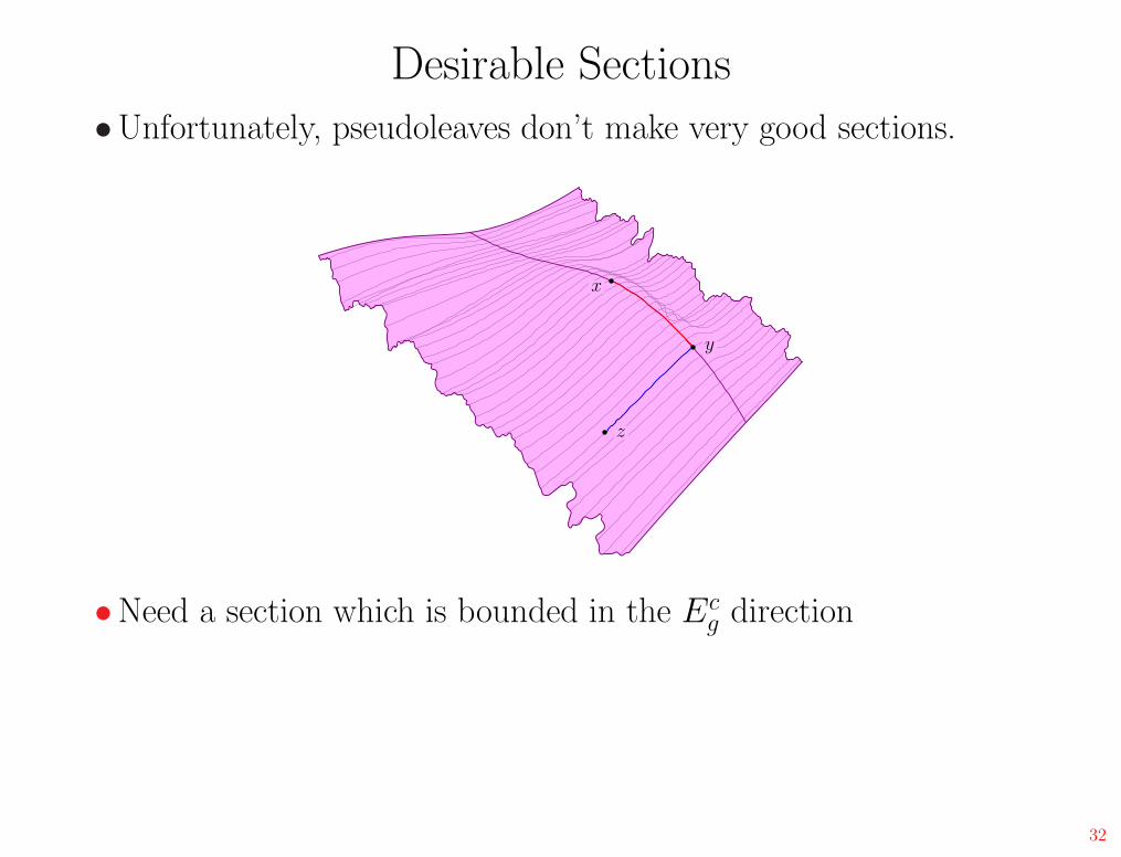
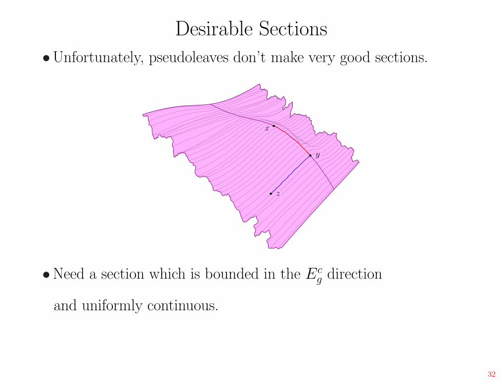
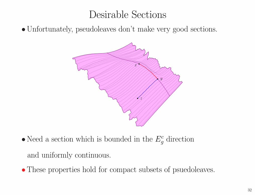
Desirable Sections
•Unfortunately, pseudoleaves don’t make very good sections.
x
y
z
32
Desirable Sections
•Unfortunately, pseudoleaves don’t make very good sections.
x
y
z
•Need a section which is bounded in the Ecg direction
32
Desirable Sections
•Unfortunately, pseudoleaves don’t make very good sections.
x
y
z
•Need a section which is bounded in the Ecg direction
and uniformly continuous.
32
Desirable Sections
•Unfortunately, pseudoleaves don’t make very good sections.
x
y
z
•Need a section which is bounded in the Ecg direction
and uniformly continuous.
•These properties hold for compact subsets of psuedoleaves.
32
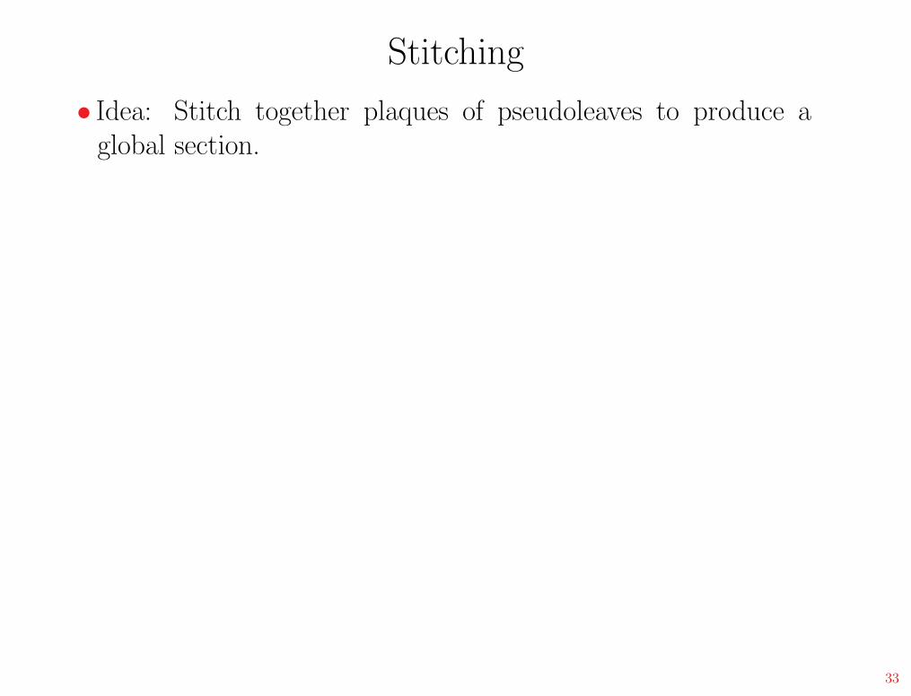
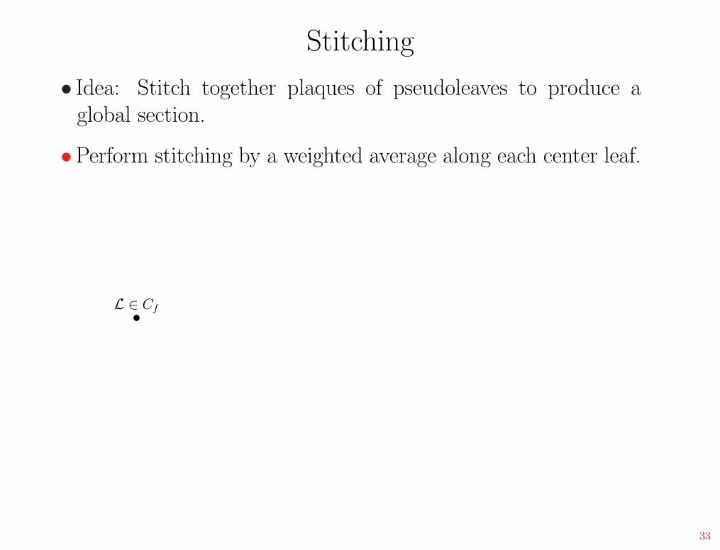
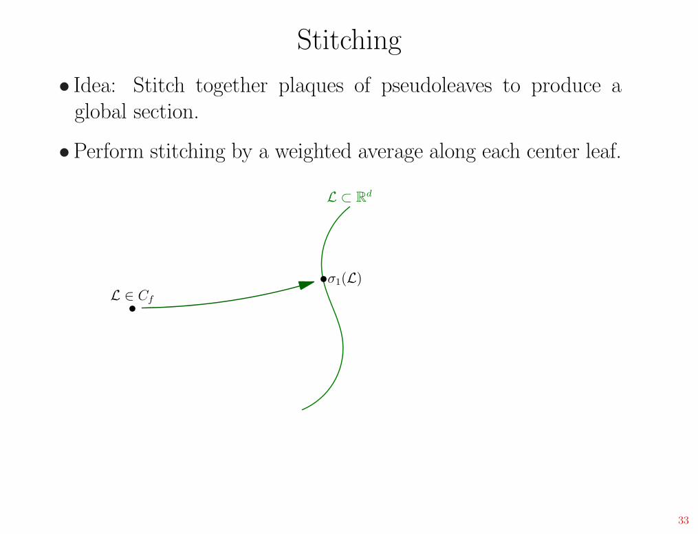
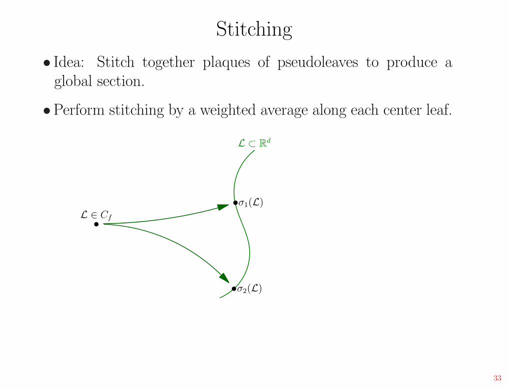
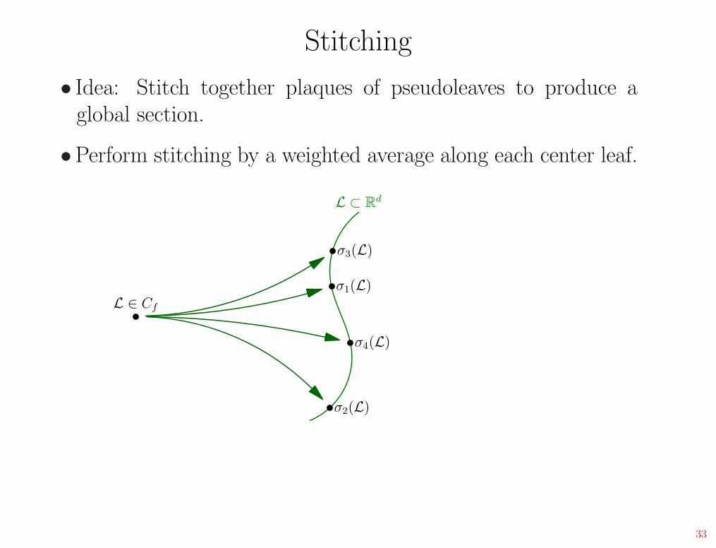
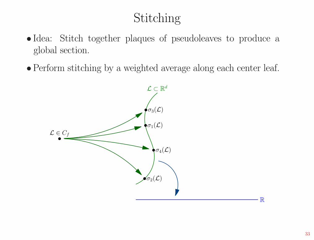
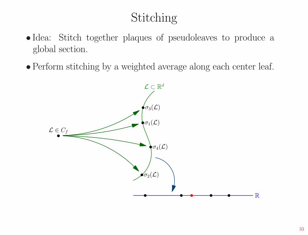
Stitching
• Idea: Stitch together plaques of pseudoleaves to produce aglobal section.
33
Stitching
• Idea: Stitch together plaques of pseudoleaves to produce aglobal section.
•Perform stitching by a weighted average along each center leaf.
L ∈ Cf
33
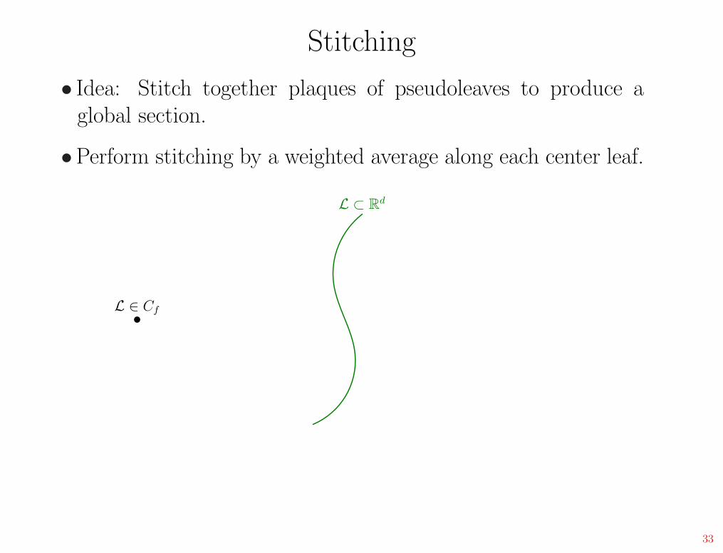
Stitching
• Idea: Stitch together plaques of pseudoleaves to produce aglobal section.
•Perform stitching by a weighted average along each center leaf.
L ∈ Cf
L ⊂ Rd
33
Stitching
• Idea: Stitch together plaques of pseudoleaves to produce aglobal section.
•Perform stitching by a weighted average along each center leaf.
L ∈ Cf
L ⊂ Rd
σ1(L)
33
Stitching
• Idea: Stitch together plaques of pseudoleaves to produce aglobal section.
•Perform stitching by a weighted average along each center leaf.
L ∈ Cf
L ⊂ Rd
σ1(L)
σ2(L)
33

Stitching
• Idea: Stitch together plaques of pseudoleaves to produce aglobal section.
•Perform stitching by a weighted average along each center leaf.
L ∈ Cf
L ⊂ Rd
σ1(L)
σ2(L)
σ3(L)
33
Stitching
• Idea: Stitch together plaques of pseudoleaves to produce aglobal section.
•Perform stitching by a weighted average along each center leaf.
L ∈ Cf
L ⊂ Rd
σ1(L)
σ2(L)
σ3(L)
σ4(L)
33
Stitching
• Idea: Stitch together plaques of pseudoleaves to produce aglobal section.
•Perform stitching by a weighted average along each center leaf.
L ∈ Cf
L ⊂ Rd
σ1(L)
σ2(L)
σ3(L)
σ4(L)
R
33

Stitching
• Idea: Stitch together plaques of pseudoleaves to produce aglobal section.
•Perform stitching by a weighted average along each center leaf.
L ∈ Cf
L ⊂ Rd
σ1(L)
σ2(L)
σ3(L)
σ4(L)
R
33
Stitching
• Idea: Stitch together plaques of pseudoleaves to produce aglobal section.
•Perform stitching by a weighted average along each center leaf.
L ∈ Cf
L ⊂ Rd
σ1(L)
σ2(L)
σ3(L)
σ4(L)
R
33

Stitching
• Idea: Stitch together plaques of pseudoleaves to produce aglobal section.
•Perform stitching by a weighted average along each center leaf.
L ∈ Cf
L ⊂ Rd
σ1(L)
σ2(L)
σ3(L)
σ4(L)
R
33
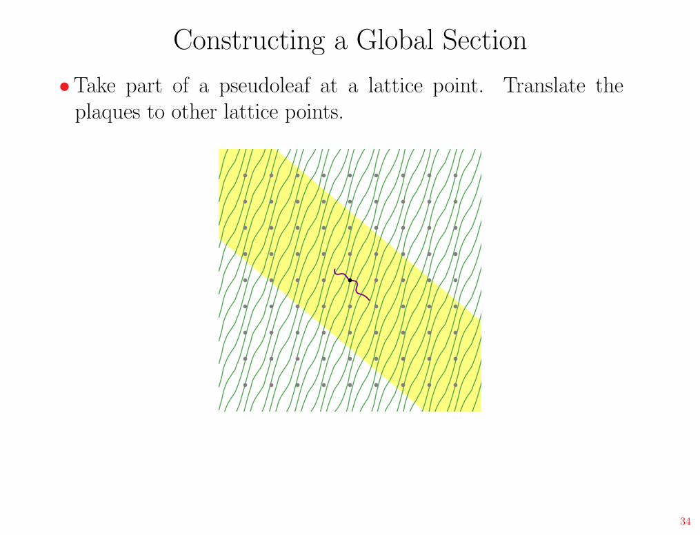
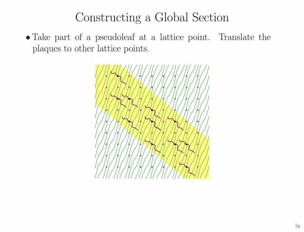
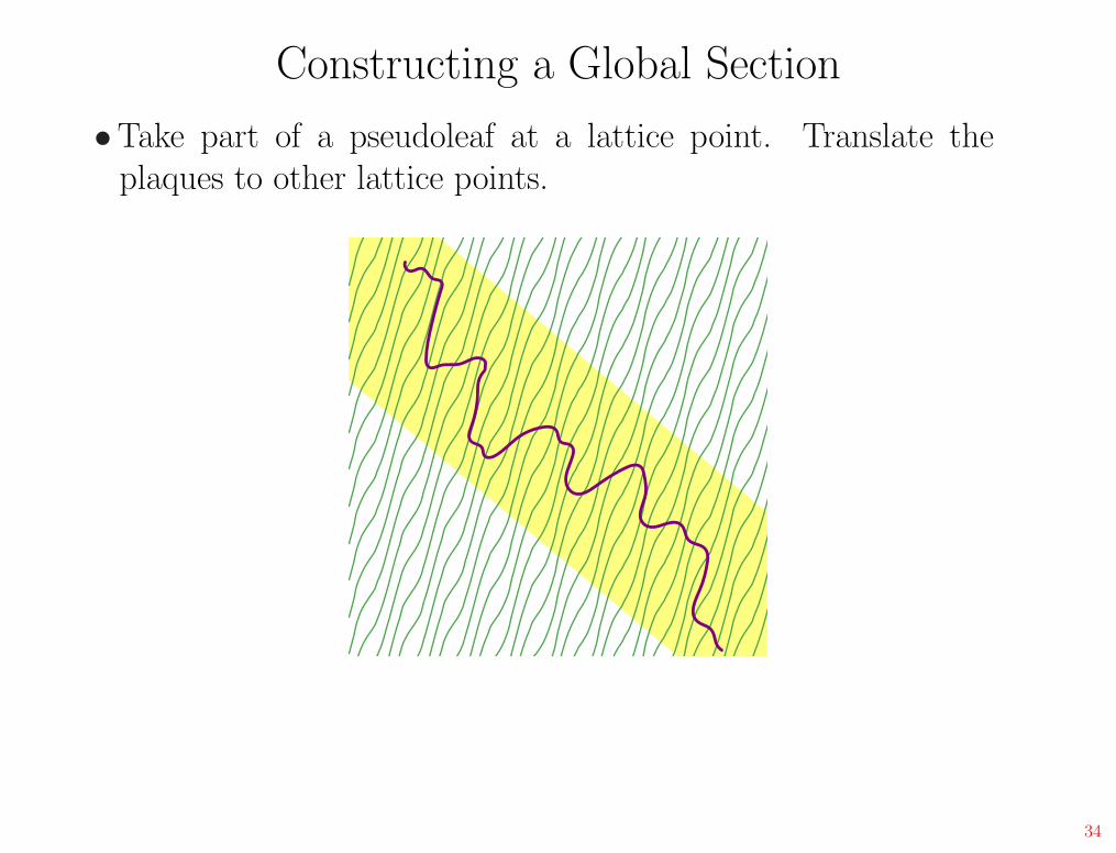
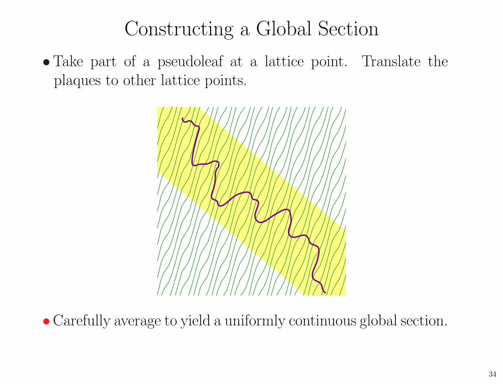
Constructing a Global Section
•Take part of a pseudoleaf at a lattice point. Translate theplaques to other lattice points.
34
Constructing a Global Section
•Take part of a pseudoleaf at a lattice point. Translate theplaques to other lattice points.
34

Constructing a Global Section
•Take part of a pseudoleaf at a lattice point. Translate theplaques to other lattice points.
34
Constructing a Global Section
•Take part of a pseudoleaf at a lattice point. Translate theplaques to other lattice points.
34
Constructing a Global Section
•Take part of a pseudoleaf at a lattice point. Translate theplaques to other lattice points.
•Carefully average to yield a uniformly continuous global section.
34

Mapping Slab to Slab
x0
35
Mapping Slab to Slab
x0
Wusg (x
0 )
35
Mapping Slab to Slab
x0
Wusg (x
0 )
σ
35
Mapping Slab to Slab
x0
Wusg (x
0 )x0 + v
σ
35
Mapping Slab to Slab
x0
Wusg (x
0 )x0 + v
Wusg (x
0 +v)
σ
35
Mapping Slab to Slab
x0
Wusg (x
0 )x0 + v
Wusg (x
0 +v)
σ
σ + v
35
Mapping Slab to Slab
x0
Wusg (x
0 )x0 + v
Wusg (x
0 +v)
σ
σ + v
35

Mapping Slab to Slab
x0
Wusg (x
0 )x0 + v
Wusg (x
0 +v)
y σ
σ + v
35
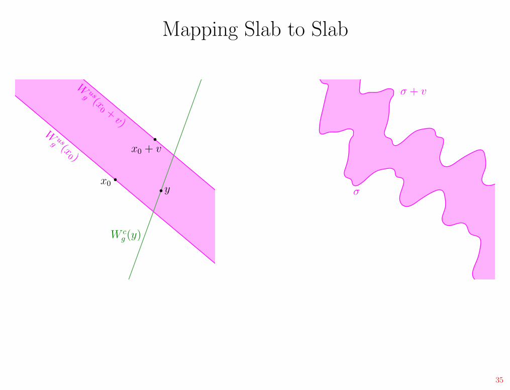
Mapping Slab to Slab
x0
Wusg (x
0 )x0 + v
Wusg (x
0 +v)
W cg (y)
y σ
σ + v
35

Mapping Slab to Slab
x0
Wusg (x
0 )x0 + v
Wusg (x
0 +v)
W cg (y)
y σ
σ + v
H(
W cg (y)
)
35

Mapping Slab to Slab
x0
Wusg (x
0 )x0 + v
Wusg (x
0 +v)
W cg (y)
y σ
σ + v
H(
W cg (y)
)
35

Mapping Slab to Slab
x0
Wusg (x
0 )x0 + v
Wusg (x
0 +v)
W cg (y)
y σ
σ + v
H(
W cg (y)
)
35

Mapping Slab to Slab
x0
Wusg (x
0 )x0 + v
Wusg (x
0 +v)
W cg (y)
y σ
σ + v
H(
W cg (y)
)
h0(y)
h0
35
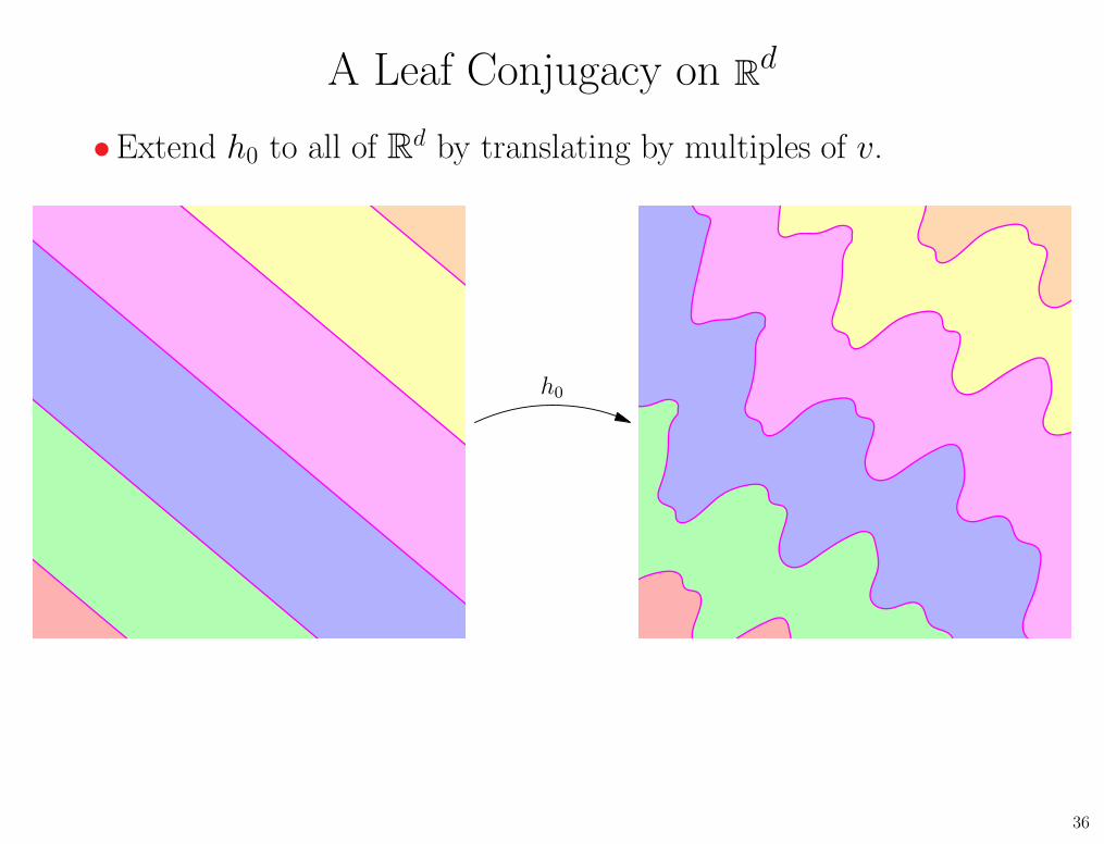
A Leaf Conjugacy on Rd
•Extend h0 to all of Rd by translating by multiples of v.
h0
36
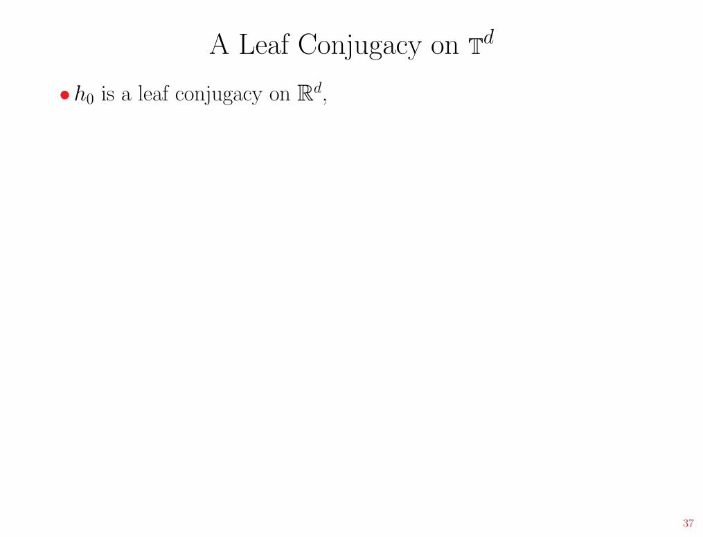
A Leaf Conjugacy on Td
•h0 is a leaf conjugacy on Rd,
37

A Leaf Conjugacy on Td
•h0 is a leaf conjugacy on Rd,
but there is no reason to think it descends to Td.
37

A Leaf Conjugacy on Td
•h0 is a leaf conjugacy on Rd,
but there is no reason to think it descends to Td.
•For z ∈ Zd, define hz : R
d → Rd as a translate of h0:
hz(x) = h0(x − z) + z.
37
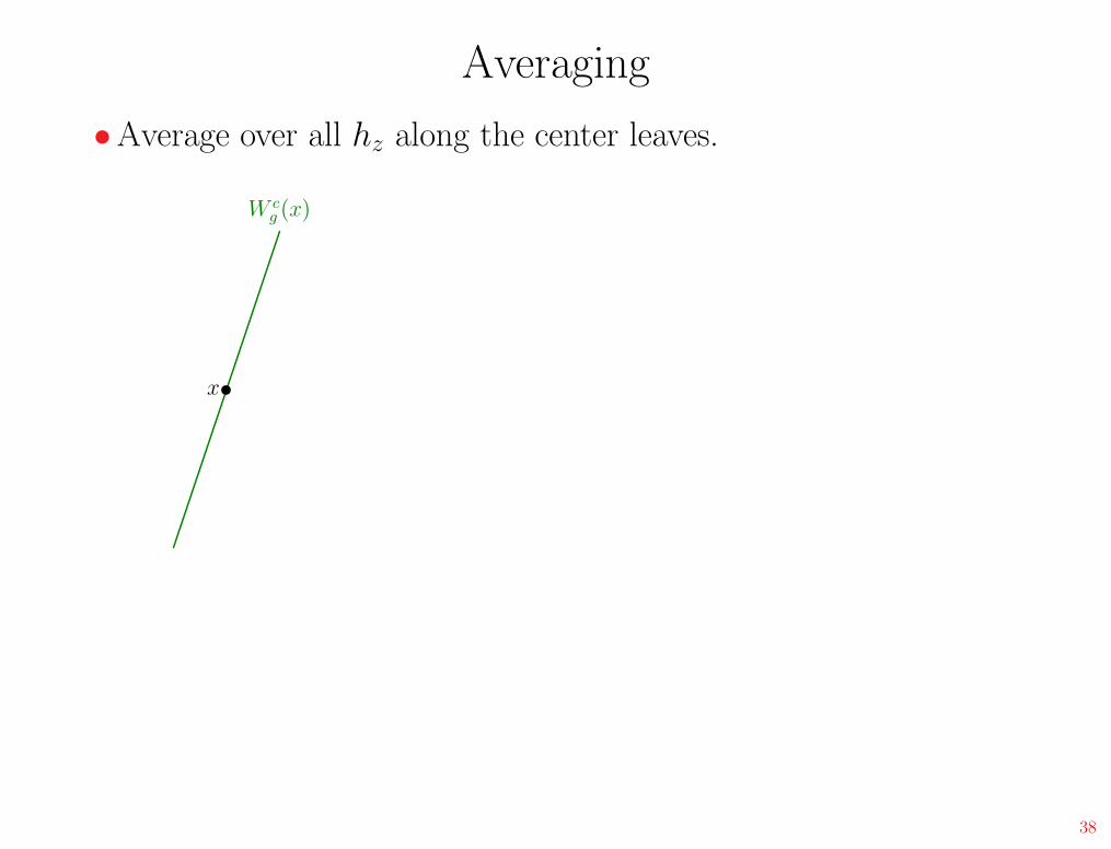
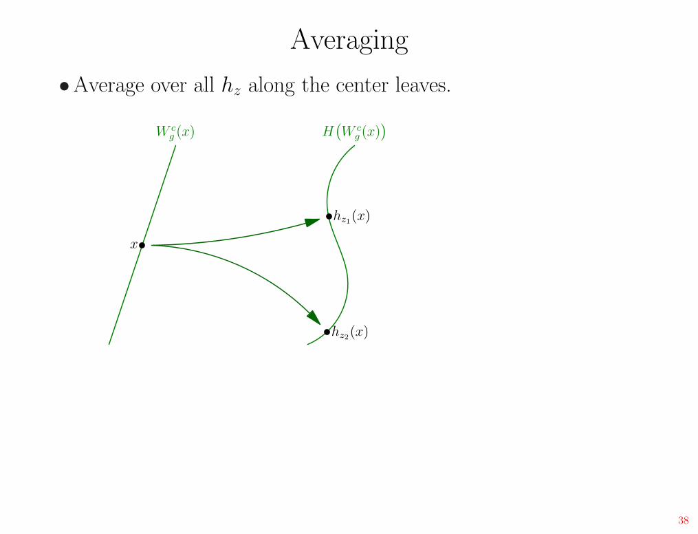
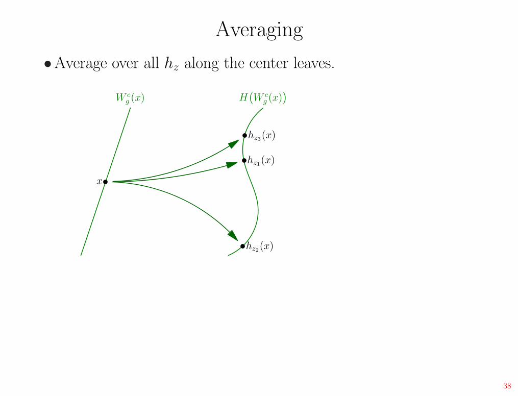
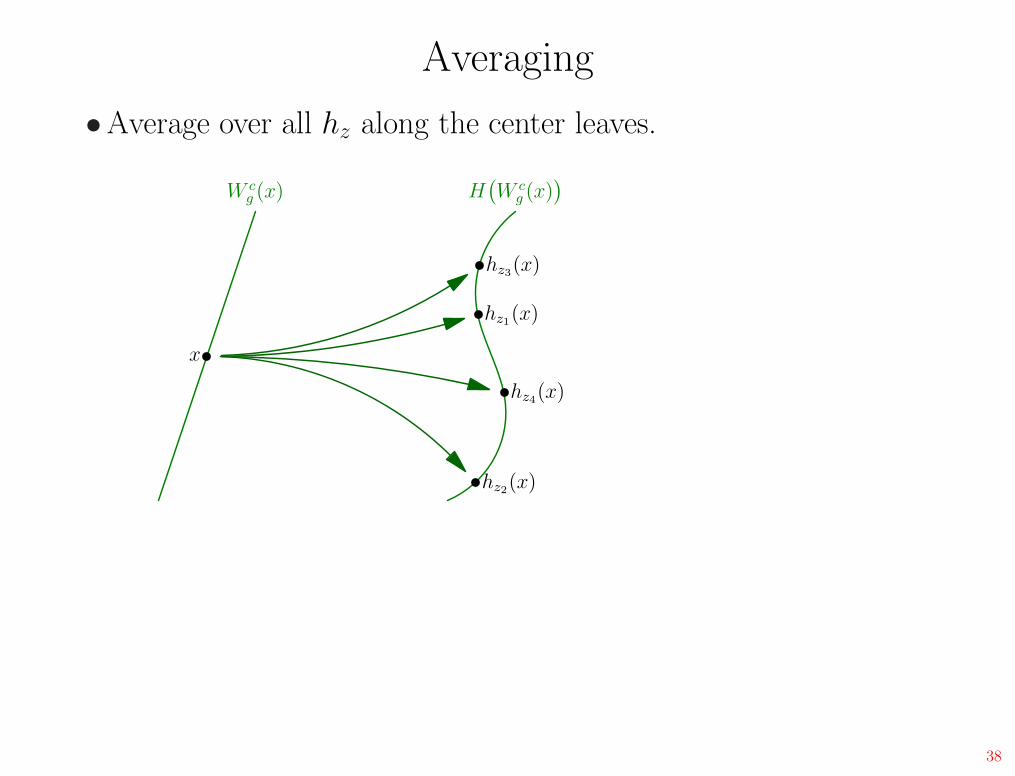
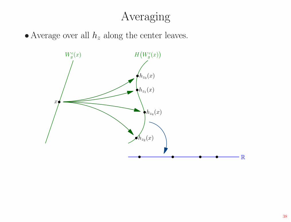
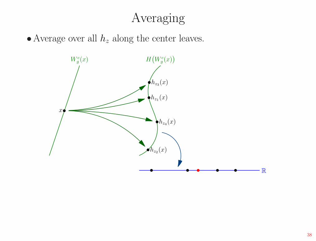
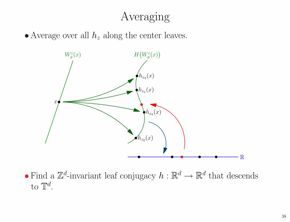
Averaging
•Average over all hz along the center leaves.
W cg (x)
x
38
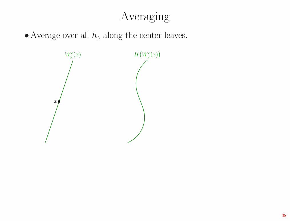
Averaging
•Average over all hz along the center leaves.
W cg (x)
x
H(
W cg (x)
)
38
Averaging
•Average over all hz along the center leaves.
W cg (x)
x
H(
W cg (x)
)
hz1(x)
38
Averaging
•Average over all hz along the center leaves.
W cg (x)
x
H(
W cg (x)
)
hz1(x)
hz2(x)
38
Averaging
•Average over all hz along the center leaves.
W cg (x)
x
H(
W cg (x)
)
hz1(x)
hz2(x)
hz3(x)
38
Averaging
•Average over all hz along the center leaves.
W cg (x)
x
H(
W cg (x)
)
hz1(x)
hz2(x)
hz3(x)
hz4(x)
38

Averaging
•Average over all hz along the center leaves.
W cg (x)
x
H(
W cg (x)
)
hz1(x)
hz2(x)
hz3(x)
hz4(x)
R
38
Averaging
•Average over all hz along the center leaves.
W cg (x)
x
H(
W cg (x)
)
hz1(x)
hz2(x)
hz3(x)
hz4(x)
R
38
Averaging
•Average over all hz along the center leaves.
W cg (x)
x
H(
W cg (x)
)
hz1(x)
hz2(x)
hz3(x)
hz4(x)
R
38
Averaging
•Average over all hz along the center leaves.
W cg (x)
x
H(
W cg (x)
)
hz1(x)
hz2(x)
hz3(x)
hz4(x)
R
38
Averaging
•Average over all hz along the center leaves.
W cg (x)
x
H(
W cg (x)
)
hz1(x)
hz2(x)
hz3(x)
hz4(x)
R
•Find a Zd-invariant leaf conjugacy h : R
d → Rd that descends
to Td.
38
Further Questions
•Franks-Manning extends to nilmanifolds and infranilmanifolds.
39
Further Questions
•Franks-Manning extends to nilmanifolds and infranilmanifolds.
•What is the partially hyperbolic extension?
39
Further Questions
•Franks-Manning extends to nilmanifolds and infranilmanifolds.
•What is the partially hyperbolic extension?
• Is dim Ecf = 1 necessary?
39
Further Questions
•Franks-Manning extends to nilmanifolds and infranilmanifolds.
•What is the partially hyperbolic extension?
• Is dim Ecf = 1 necessary?
• Is quasi-isometry necessary? Is it redundant for tori?
39
Further Questions
•Franks-Manning extends to nilmanifolds and infranilmanifolds.
•What is the partially hyperbolic extension?
• Is dim Ecf = 1 necessary?
• Is quasi-isometry necessary? Is it redundant for tori?
•Can we classify all partially hyperbolic diffeomorphisms on 3-manifolds?
39
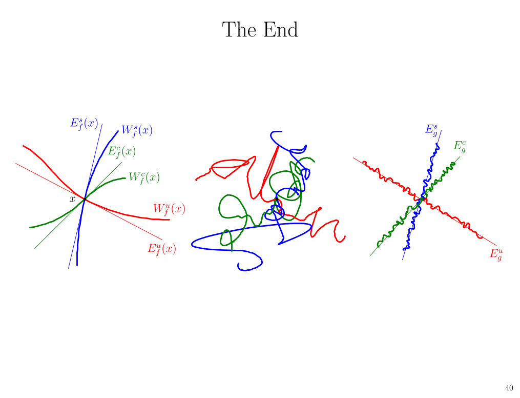
The End
Euf (x)
Esf (x)
Ecf (x)
xW u
f (x)
W sf (x)
W cf (x)
Eug
Esg
Ecg
40
Asymptote: 2D & 3D Vector Graphics Language
symptotesymptotesymptotesymptotesymptotesymptotesymptotesymptotesymptotesymptotesymptote
http://asymptote.sf.net
(freely available under the GNU public license)
41