leadership in public good provision: a timing game ... - cerdi
TRANSCRIPT
Etudes et Documents 2008.17
Leadership in Public Good Provision: a Timing
Game Perspective
Hubert Kempf and Grégoire Rota Graziosi‡
: Banque de France and Paris School of Economics
Mail address: Centre d’Economie de la Sorbonne, Université Paris-1 Panthéon-Sorbonne,
65 boulevard de l’Hôpital, 75013 Paris, France.
Email: [email protected]
‡: CERDI-CNRS, Université d’Auvergne,
Mail address: 65 boulevard François Mitterrand, 63000 Clermont-Ferrand, France
Email: [email protected]
December 5, 2008
2
Abstract
We address in this paper the issue of leadership when two governments provide
public goods to their constituencies with cross border externalities as both public
goods are valued by consumers in both countries. We study a timing game be-
tween two di erent countries: before providing public goods, the two policymakers
non-cooperatively decide their preferred sequence of moves. We establish conditions
under which a Þrst- or second-mover advantage emerges for each country, highlight-
ing the role of spillovers and the strategic complementarity or substitutability of
public goods. As a result we are able to prove that there is no leader when, for both
countries, public goods are substitutable. When public goods are complements for
both countries, both countries may emerge as the leader in the game. Hence a co-
ordination issue arises. We use the notion of risk-dominance to select the leading
government. Lastly, in the mixed case, the government for whom public goods are
substitutable becomes the leader.
1 Introduction
The issue of leadership is much studied in industrial economics, in particular in
relation with duopoly theory, but much less in public economics. Yet this issue
cannot be under-estimated in this domain of economics. There are many examples
of interdependent decisions made by independent public authorities. To name a few
examples, let us mention the case of cross-border externalities, federations, military
alliances, environmental issues, transnational public goods. These public authorities
rule clearly di erentiated jurisdictions. It is common to oppose core vs periphery
jurisdictions, large vs small governments, or di erences in capacities (in military
alliances for example). These di erences often translate in strategic asymmetries,
as one jurisdiction assumes a leading role with respect to others, setting the agenda,
deciding and constraining other jurisdictions, considered and acting as followers.
The present paper aims at formally addressing the issue of leadership in public
economics, focusing on the problem of providing public goods in the presence of
cross-jurisdiction spillovers.1 We aim at understanding who is leader (follower) in
providing public goods and why. We also want to characterize the consequences
of leadership relative to its absence for each jurisdiction involved in this setting.
In order to answer this question, we adopt a game-theoretic approach and deÞne
leadership as the action of moving Þrst.2
As our approach is parallel to the one adopted in industrial economics to study
leadership in duopolies, a brief summary of this research is relevant here.3 First, tak-
ing as given the order of moves in a duopoly, in other words the presence of a leader,
industrial economists were interested in assessing the respective advantages of each
Þrm: that is, in comparing the Þrst-mover and second-mover advantages, deÞned as
1Of course, there are many more issues in public economics which can be related to the problemof leadership. We return to this point in the conclusion.
2See Kempf and Taugourdeau (2005) for a Þrst exploration of Stackelberg games over Þscaldecisions in a two-country model.
3Vives (1999) provides a survey of this literature.
1
the payo s for this Þrm of playing either Þrst or second. Once it was recognized that
the two roles of leader and follower lead to di erent advantages, the next step was to
attempt to endogenize the moves, that is consider the sequence of moves as the equi-
librium result of non-cooperating strategies played by the two Þrms given their own
relative characteristics and their prospective advantage as a leader or as a follower.
d’Aspremont and Gerard-Varet (1980), Gal-Or (1985) and Dowrick (1986) proposed
an initial analysis, which has been extended by Hamilton and Slutsky (1990), Pal
(1996), Amir and Grilo (1999), van Damme and Hurkens (1999) and more recently
by van Damme and Hurkens (2004) or Amir and Stepanova (2006). The determina-
tion of simultaneity versus sequentiality of moves, as well as the assignment of roles
of the players in the latter case, is then completely endogenous.
In this paper, we shall follow the same logic. First, using a simple yet fairly
general two-jurisdiction model of public good provision and externalities (linked
to the public goods) across jurisdictions, we shall characterize the Þrst-mover and
second-mover advantages. Then we shall set-up a timing game, or equivalently the
two-period action commitment game proposed by Hamilton and Slutsky (1990). In
the Þrst stage, the policymaker of each jurisdiction states which role (leading or fol-
lowing) it prefers. Once the solution of this stage is obtained, that is when the two
roles are attributed to the two jurisdictions, given their statements, the resulting
game is played in the second stage of the timing game.4 It may happen that two
equilibria emerge as the outcome of the Þrst stage: that is, two sequences of moves
are solutions of the two-stage game. In this case, in order to break-up this multiplic-
ity, we resort to the concepts of Pareto-dominance and risk-dominance o ered by
Harsanyi and Selten (1988). Applying this concept to two di erent speciÞcations of
our general model, we show how it allows a simple and straightforward explanation
4Another presentation of this game has been proposed by van Damme and Hurkens (1999):each player has to move in one of two periods; choices are simultaneous, but if one player chooseto move early while the other moves late, the latter behaves as a Stackelberg follower, the formeras a leader.
2
of which jurisdiction ends up as the leader.
We prove that both the magnitude of the moves’ advantages and the existence
and identity of a leader depend on the characteristics of public goods in the utility
function. When for both countries the public goods are substitutes, both juris-
dictions experience a Þrst-mover advantage and the solution of the timing game is
the Nash simultaneous game. When for both countries the public goods are comple-
ments, at least one jurisdiction beneÞts from a second-mover advantage when public
goods are complements and the two sequential “basic games” are solutions of the
timing game. Finally, in the mixed case, the country for which the public goods are
substitutes beneÞts from a Þrst-mover advantage and is the leader. Then we prove
that the use of the risk-dominance criterion always allows us to identify the leader
and provides an explanation of this leadership in each of the two speciÞcations of the
utility function we consider. Overall, the issue of leadership is solved for all cases.
Our work refers to the study of inter-jurisdictional spillovers. Several recent con-
tributions can be questioned through our results. The literature on centralization
and international unions only considers simultaneous games where countries choose
to cooperate or not (see for instance, Lockwood (2002), Besley and Coate (2003)
or Alesina, Angeloni, and Etro (2005)). It can be deduced from our analysis that
the usual benchmark used to appreciate political centralization, i.e. the simulta-
neous Nash equilibrium, may not be relevant when public goods are complements.
The works on global public goods (Kaul, Grunberg, and Stern (1999) or Barrett
(2007)) are also related to our analysis since we establish a taxonomy of interna-
tional spillovers and their consequences in term of their global provision and the
“natural” (since endogenous) emergence of a leader. We emphasize that the free
rider issue is not as strong as predicted in the literature, when public goods are
complements. Indeed, in this situation, a sequential situation emerges as a Sub-
game Perfect Equilibrium (SPE), which involves a higher provision of public goods
3
to this at the simultaneous Nash equilibrium.5
Finally, our analysis might be fruitful in political science where the concepts
of hegemony and leadership, often confounded, remain a hot topic (see Keohane
(1984) or Pahre (1999)). By considering the leadership as endogenous, we are able to
formalize a clear distinction between hegemony and leadership: hegemony would be
a structural variable (an ad hoc assumption in the utility functions), while leadership
would characterize the solution of a timing game.
The next section sets up the two-jurisdiction model we use and studies the three
non-cooperating games, with either synchronous or sequential moves, that can be
played, and derives the Þrst- and second-mover advantages for a very general speci-
Þcation of the utility function. The third section tackles the selection of a leader by
means of a timing game, relying when necessary on the concept of risk-dominance.
The last section concludes.
2 Public good provision non-cooperating games.
We consider an economy consisting of two jurisdictions or countries (! and ").
There is no mobility accross countries. Their populations are normalized to 1. Each
country # ( {!$"}) provides a local public good, in quantity % , which generates
some externalities for the other country, namely country & (6= #). There is perfect
information. Inhabitants in country # are assumed to have preferences that can be
5Our analysis may also be linked to the work of Varian (1994), who considers a sequentialgame of private contribution. This author highlights that the ability to commit to a contributionreinforces the free-rider problem and he concludes that the amount of public good sequentiallyprovided is never larger than the amount simultaneously provided. We extend his analysis in twoways: Þrst we consider the leader as endogenous; second, since Varian (1994) focuses exclusivelyon the contribution game proposed by Bergstrom, Blume, and Varian (1986), he considers onlypublic goods as substitutes, we study here all the possible conÞgurations. Whereas the conclusionsof Varian (1994) remain valid for substitutes and an endogenous leadership, they do not holdanymore as soon as complement public goods considered.
4
described by the following utility function:
' (% $ %!) = ( ! % + (% $ %!) )
The function (% $ %!) represents the public goods provision function, entering lin-
early into the utility function of the representative agent in country &) We make the
following assumptions:
"# = !$"$ 1 (% $ %!) #
" (# $#!)
"# * 0$
2 (% $ %!) 0$
11 (% $ %!) + 0$
12 (% $ %!) 0)
The derivative 12 (% $ %!) plays a crucial role in this paper. When for any (% $ %!),
12 (% $ %!) is positive, we shall say that the two public goods are complements: an
increase in the provision of %! increases the marginal utility of good % ) When it is
negative, they are substitutes. When it is nil, the three studied games yield the
same equilibrium payo s. This last assumption is often implicit in the literature on
inter-jurisdictional spillovers and it appears as an important limit to these analysis
(see for instance Lockwood (2002), Besley and Coate (2003) or Dur and Roelfsema
(2005)).6
Despite the use of a quasi-linear utility function which is the workhorse of this
literature (see Batina and Ihori (2005)), our formalization remains relatively general
with respect to the quoted works. It allows us to encompass several works con-
cerning transnational or global public goods provisions, international organizations
or Þscal federalism where the jurisdiction correspond to subnational governments.
Moreover, the quasi-linear form involves a strict equivalence between the function
1 (% $ %!) and the marginal rate of substitution (MRS) between private and public
consumptions in country #.
6Lockwood (2002) speciÞes (! " !!) = ! + !! ; Besley and Coate (2003), (! " !!) =(1! #) log ! + # log !! with # [0" 1]; Dur and Roelfsema (2005), (! " !!) = $ (! ) + #$ (!!).
5
We consider three possible situations for the determination of non-cooperative
national policies, deÞning three “basic games”: the simultaneous Nash game (,%)
and the two Stackelberg games (,& where country # is leader and country & follower).
2.1 Characterizing the simultaneous game (,%).
At the simultaneous non-cooperative equilibrium, each country chooses its own pol-
icy taking as given the provision of the other public good, that without taking in
account the externalities its decision creates on the other country. We denote by¡%%' $ %%
(
¢the Nash equilibrium of this game. This pair must verify the following set
of deÞnitions: !!"
!!#
%%' # argmax
#">0'' (%'$ %() $ %( given,
%%( # argmax
##>0'( (%($ %') $ %' given.
The non-cooperative equilibrium levels of public good provisions are implicitly given
by:
"# {!$"} $ !1 + 1
¡%% $ %%
!
¢= 0 (1)
Following Vives (1999), a su!cient condition for the best-replies to be contractions
is:"2) (# $#!)
"#2 +¯̄¯"
2) (# $#!)
"# "#!
¯̄¯ + 0, which yields in our model
11 (% $ %!) +
¯̄
12 (% $ %!)
¯̄+ 0$ (2)
This insures the existence and the unicity of the Nash Equilibrium. In the following,
we always assume that condition (2) is satisÞed.
2.2 Characterizing the Stackelberg game (,&' ).
Under this scenario, we assume that one of the two jurisdictions denoted by # is the
Þrst player to set its provision of % $ and then jurisdiction & (the follower - ) chooses
6
its own level % . In other words, jurisdiction behaves as a Stackelberg leader (!).
Applying backward induction, we Þrst consider the maximization program of the
follower which is given by:
"! ("") argmax
# # (" $ "") $ "" given.
The FOC, which is equivalent to (1) for country %, yields:
!1 + 1
¡"! ("") $ ""
¢= 0 (3)
Applying the envelop theorem, we remark that:
&"
&""
= !
12 (" $ "")
11 (" $ "")
0" 12 (" $ "") 0
The leader solves the following program:
"$" argmax
#!#"
¡""$ "
! ("")
¢
which implies the following FOC:
!1 + "1
¡"$" $ "!
¡"$"
¢¢+
&"! ("")
&""
"2
¡"$" $ "!
¡"$"
¢¢= 0
or equivalently,
!1 + "1
¡"$" $ "!
¡"$"
¢¢!
12
¡"!
¡"$"
¢$ "$
"
¢
11
¡"! ("
$" ) $ "
$"
¢ "2
¡"$" $ "!
¡"$"
¢¢= 0 (4)
The SOC is assumed to be satisÞed.
7
2.3 Comparison of the levels of public good provisions.
Our analysis o ers a taxonomy of inter-jurisdictional interactions. Indeed, we con-
sider six cases depending on the sign of the spillovers and the presence of comple-
mentarity or substitutability among national public goods.7 The literature focuses
essentially on one kind of interactions, when either complementarity or substitutabil-
ity is considered.8 Indeed, many authors implicitly assume a standard technology of
agregation of jurisdiction’s contribution, the weighted summation, which may be re-
lied to the canonical model of Bergstrom, Blume, and Varian (1986). This hypothesis
involves substitutability among national public goods. Thus, the standard formal-
ization of interjurisdictional interactions corresponds to the case where "% 2 (') ( 0
and "% 12 (') ) 0. Under these assumptions, Bloch and Zenginobuz (2007) renewes
the analysis of the issue of local public good provision with spillovers and highlights
their e ects. Ellingsen (1998), Redoano and Scharf (2004), and Alesina, Angeloni,
and Etro (2005) consider the issues of international agreements or centralization
under similar assumptions.9
Hirshleifer (1983)10 proposed two other agregation technologies: the “weakest-
link” and the “best-shot”. These functions have been used in the context of global
public goods (see Kaul, Grunberg, and Stern (1999) or Barrett (2007)). These two
cases generate several di!culties since the underlying functions are not di eren-
tiable. Cornes (1993) proposed a class of functions which encompasses the di erent
preceeding cases. Cornes and Hartley (2007) renewes the analysis of Bergstrom,
Blume, and Varian (1986) by considering a CES composition function. The case
of complements and positive spillovers ( "% 2 (') ( 0 and "%
12 (') ( 0) might then
correspond to the analysis of defence expenditures between two allied countries (see
7We do not assume that the signs of the spillovers di er for the two countries.8Several papers assume functional forms such that !"
12 ( ) = 0.9These authors use a more restrictive function than our, since they assume:
(! " !") =# (!1 + $!2), with 0 % $ % 1 and #00 ( ) % 0
10See Hirshleifer (1985) for a correction.
8
Ihori (2000)) and some works on the global public goods, higlighting a better-shot
agregation technology (see Barrett (2007)). Finally, to our knowledge, the mixed
cases have not been considered in the literature. Di erent public goods can logically
be linked to di erent cases, depending on their complementarity or substitutability
and the sign of their induced spillovers. For example, national programs on airÞeld
infrastructure building can be considered as complementary and generating positive
externalities. On the other hand, national plans for biodiversity conservation can
be substitutes and related to positive externalities.
The comparison of the levels of public goods requires to consider six cases de-
pending on the sign of 2 (') and 12 (') (when it is assumed to be non-null).11 In
the appendix, we establish the following Proposition:
Proposition 1 The public good provision levels solutions of the Nash and Stackel-berg games are such that:(i) If "
2 (') ( 0 and "12 (') ( 0 (positive spillovers and complements):
½"$" ( "!
" ( "&"
"$ ( "!
( "&
or
½"$" ( "!
" ( "&"
"! ( "$
( "&
(ii) If "2 (') ) 0 and "
12 (') ( 0 (negative spillovers and complements):
½"&" ( "!
" ( "$"
"& ( "!
( "$
or
½"&" ( "$
" ( "!"
"& ( "!
( "$
(iii) If "2 (') ( 0 and "
12 (') ) 0 (positive spillovers and substitutes):
½"!" ( "&
" ( "$"
"! ( "&
( "$
(iv) If "2 (') ) 0 and "
12 (') ) 0 (negative spillovers and substitutes):
½"$" ( "&
" ( "!"
"$ ( "&
( "!
'
(v) If "% 2 (') ( 0 and "
12 (') ( 0 ( 12 (') (positive spillovers for both countries,
11The equilibria of the di erent games are identical when 12 ( ) = 0, that is in the absence of
any interaction between the two countries.
9
complements for country and substitutes for country %):
½"!" ( "&
" ( "$"
"$ ( "!
( "&
or
½"!" ( "&
" ( "$"
"! ( "$
( "&
(vi) If "% 2 (') ) 0 and "
12 (') ( 0 ( 12 (') (negative spillovers for both countries,
complements for country and substitutes for country %):
½"$" ( "&
" ( "!"
"& ( "$
( "!
or
½"$" ( "&
" ( "!"
"& ( "!
( "$
Proof. See Appendix A.1.
Consider the Þrst case ( "2 (') ( 0 and "
12 (') ( 0). When the leader, say *$
increases its level of provision relative to the Nash equilibrium value, it induces
its follower, +$ to increase its own provision level because of the complementarity
property between the two public goods. In turn, this increases the leader’s payo
because of the positive externality assumption. Hence we get "$' ( "&
' and "!( ( "&
( '
However it may happen that "!' ( "$
'' This comes from the di erences in the
" (""$ " ) functions. It may happen that the externalities and interaction e ects are
much stronger from + to *$ than from * to +' Then "$' is very close to "&
' and "$(
is very far from "&( as well as "!
' from "&' ' This explains the two possible rankings
obtained for ( ). The other cases may be explained by means of similar reasonings,
that is by the interplay between the externality e ect and the interaction e ect.
When the two countries are symmetric, that is when " (""$ " ) = (""$ " ) $ # $
the mixed cases disappear. It is immediate to derive from the previous proposition
the comparison between the public good provisions under this assumption:
Corollary 1 When " (""$ " ) = (""$ " ) $ # $ the public good provision levels solu-tions of the Nash and Stackelberg games are such that:
(i) If 2 (') ( 0 and 12 (') ( 0 (positive spillovers and complements):
"$ ( "! ( "& $
(ii) If 2 (') ) 0 and 12 (') ( 0 (negative spillovers and complements):
"& ( "! ( "$$
10
(iii) If 2 (') ( 0 and 12 (') ) 0 (positive spillovers and substitutes):
"! ( "& ( "$$
(iv) If 2 (') ) 0 and 12 (') ) 0 (negative spillovers and substitutes):
"$ ( "& ( "! '
Proof. See Appendix A.1.
This proposition can be explained following the same reasoning as for the previ-
ous proposition. We notice that the coexistence of two rankings in cases ( ) and ( )
disappears with the asymmetries between the two " (""$ " ) functions.
2.4 First-mover and second-mover advantages.
Given these rankings, we can compute the Þrst- and second-mover advantages. These
advantages has been extensively used and discussed in the duopoly theory.12 Here
they will allow us to understand the stakes linked to the possible existence of lead-
ership in public good provision. Following Amir and Stepanova (2006) we deÞne the
notions of “Þrst-” and “second-mover advantage” as follows:
DeÞnition 1 Country has a Þrst-mover advantage (a second-mover advantage) ifits equilibrium payo in the Stackelberg game in which it leads, denoted by ,)
" , ishigher (lower) than in the Stackelberg game in which it follows (,)
).
Formally, country beneÞts from a Þrst-mover advantage when
#"
¡"$" $ "!
¢( #"
¡"!" $ "$
¢
and from a second-mover advantage when
#"
¡"!" $ "$
¢( #"
¡"$" $ "!
¢'
Given this deÞnition we o er the following Proposition:
12See Bagwell and Wolinsky (2002).
11
Proposition 2 (i) If public goods are complements in both countries ( "12 (') ( 0),
at least one country has a second-mover advantage;(ii) If public goods are substitutes in both countries ( "
12 (') ) 0), each country hasa Þrst-mover advantage;(iii) If "
12 (') ( 0 ( 12 ('), country %, the country for which the public goods are
substitutes, has a Þrst-mover advantage. Country has a Þrst-mover advantage (asecond-mover advantage) when externalities from the foreign public good are positive(negative).
Proof. see Appendix A.2.
Let us Þrst focus on the case when the public goods are complements for both
countries (though a ecting them di erently) and spillovers are positive. At least one
player prefers to be a second-mover as then, it optimally beneÞts from the higher
provision decided by the Þrst-mover, which generate positive externalities. To be
second-mover allows this country to reduce its own provision of public good, in other
terms it free-rides the leader. However this free-riding is less than in the simultaneous
Nash game where spillovers are positive. The other cases can be explained by similar
reasonings. In the case of substitutable public goods and positive spillovers, which
is the case studied by Varian (1994), our result is consistent with his.
3 Selecting a leader through a timing game.
We have just seen that the existence and identity of a leader matters because of Þrst-
or second-mover advantages. This puts to the fore the issue of determining whether
a leader emerges, and if yes, its identity. In order to address this issue, we want to
endogenously deÞne the order of moves, and not take it as given as in the previous
section by resorting to a timing game, following the seminal study of Hamilton and
Slutsky (1990).
A timing game is a sequential game in the Þrst stage of which players non-
cooperatively choose their preferred order of moves. Once the order of moves has
been deÞned, players act accordingly in the second stage, that is non-cooperatively
12

choose their level of public good provision, applying the order of moves selected
in the Þrst stage. In other words, a timing game is an extended game e which
encompasses the preceding games. Following Hamilton and Slutsky (1990) and
Amir and Stepanova (2006) we restrict our attention to the SPE of e .
More precisely, e is deÞned as follows: at the Þrst or preplay stage to the “basic
game”, players simultaneously and independently of each other decide whether they
prefer to move early or late in the “basic game”. In the same way as Hamilton and
Slutsky (1990), we assume that if country ! chooses leadership (strategy Leads), it
commits itself to setting its national policy as leader and if it chooses to be a follower
(Follows), it commits itself to following the other country’s decision. Once the timing
choice of each player is announced, the order of moves is deÞned according to the
following rules: if countries choose complementary roles, there preferred moves are
enforced and one of the two possible Stackelberg games will emerge. If both choose
lead or follow, as their decisions are inconsistent, it is decided that the simultaneous
non-cooperative game will be enforced. That is, the second stage corresponds to the
realization of the selected “basic game”: it is one of the three games studied in the
previous section.
Notice that, in choosing their role (leader or follower), the two players also choose
which kind of behavior they prefer. Therefore this game has the following normal
form:13
Country "
Leads Follows
Country # Leads $ ! % $ " $#! % $
$"
Follows $$! % $#" $ ! % $
"
13We remark that the literature on endogenous timing remains divided to qualify the situationwhere both players choose to lead. Indeed, Dowrick (1986) and more recently van Damme andHurkens (1999) consider a Stackelberg warfare, where both countries apply their action as a leader.In contrast, Hamilton and Slutsky (1990) or Amir and Stepanova (2006) apprehend this situationas the static Nash game. Hamilton and Slutsky (1990) (p. 42) emphasize that Stackelberg warfarecan occur only through error, since the underlying strategy of one player is not consistent with theother player’s strategy.
13
where $ % = $%¡& % % &
%
¢, $$% = $%
¡&$% % &
#%
¢and $#% = $%
¡&#% % &
$%
¢.
3.1 Solutions to the leadership problem.
The solution to this reduced form game is equivalent to characterizing the solution
to the leadership problem. There is no leader when both government choose the
same action; a leader emerges when they choose complementary roles. The result
of the timing game can be related to the nature of the interactions between the two
countries. We obtain the following Proposition:
Proposition 3 (i) If public goods are complements, the subgame perfect equilibriaare the two Stackelberg situations whatever is the sign of spillovers;(ii) If public goods are substitutes, the subgame perfect equilibrium is the simultane-ous moves situation whatever is the sign of spillovers;(iii) If public goods are complements for country ! and substitutes for country ', thesubgame perfect equilibrium is the Stackelberg situation where country ' leads andcountry ! follows whatever is the sign of spillovers.
Proof. See Appendix A.3.
14
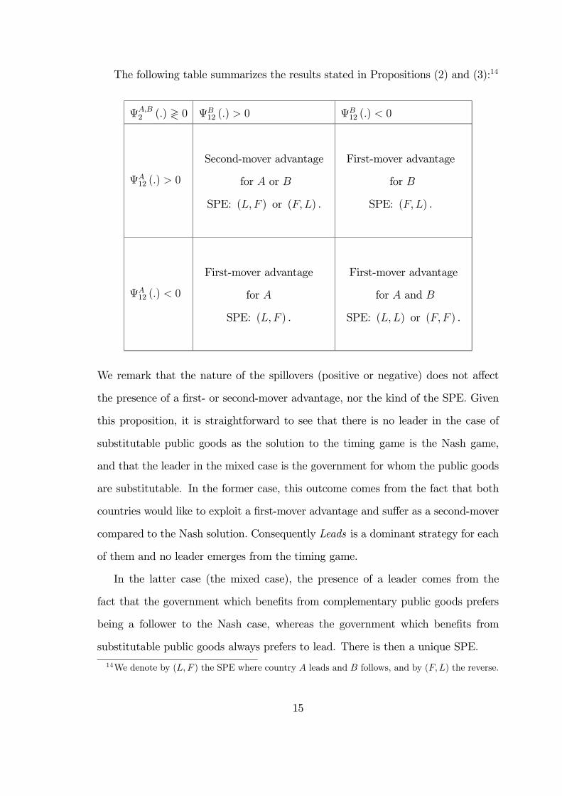
The following table summarizes the results stated in Propositions (2) and (3):14
!&"2 (() 0
"12 (() ) 0
"12 (() * 0
!12 (() ) 0
Second-mover advantage
for # or "
SPE: (+%, ) or (,%+) .
First-mover advantage
for "
SPE: (,%+) .
!12 (() * 0
First-mover advantage
for #
SPE: (+%, ) .
First-mover advantage
for # and "
SPE: (+%+) or (,%, ) .
We remark that the nature of the spillovers (positive or negative) does not a ect
the presence of a Þrst- or second-mover advantage, nor the kind of the SPE. Given
this proposition, it is straightforward to see that there is no leader in the case of
substitutable public goods as the solution to the timing game is the Nash game,
and that the leader in the mixed case is the government for whom the public goods
are substitutable. In the former case, this outcome comes from the fact that both
countries would like to exploit a Þrst-mover advantage and su er as a second-mover
compared to the Nash solution. Consequently Leads is a dominant strategy for each
of them and no leader emerges from the timing game.
In the latter case (the mixed case), the presence of a leader comes from the
fact that the government which beneÞts from complementary public goods prefers
being a follower to the Nash case, whereas the government which beneÞts from
substitutable public goods always prefers to lead. There is then a unique SPE.
14We denote by ( !" ) the SPE where country # leads and $ follows, and by ("! ) the reverse.
15
On the other hand, when the public goods are complements, there are two pos-
sible Stackelberg equilibria solutions to the timing game. This comes from the fact
that in any possible case with complement public goods, both the Þrst- and second-
movers are better o than under a Nash equilibrium. This raises a coordination
issue: how to solve the tie? In the next section, we provide a solution for the
selection of a leader by means of the risk-dominance criterion.
3.2 Selecting a leader in the complementarity case.
To solve the coordination issue when the public goods are complements, more for-
mally, when %12 (() ) 0% two criteria can be used for the selection of the leader in
this case: the Pareto-dominance and the risk-dominance. Given Proposition 2, it
is clear that no equilibrium Pareto-dominates the other one when both Þrms have a
second-mover advantage. Hence, following Harsanyi and Selten (1988), we have to
turn to the risk-dominance criterion. It amounts to a minimization of the risk of a
coordination failure due to strategic uncertainty.15
Harsanyi and Selten (1988) deÞne the concept of risk-dominance as follows:
DeÞnition 2 An equilibrium risk-dominates another equilibrium when the formeris less risky than the latter, that is the risk-dominant equilibrium is the one for whichthe product of the deviation losses is the largest.
Risk-dominance allows a simple characterization for 2× 2 games with two Nash
equilibria: the equilibrium (A Leads, B Follows) risk-dominates the equilibrium (A
Follows, B Leads) if the former is associated with the larger product of deviation
losses. More formally, we have: (A Leads, B Follows) risk-dominates (A Follows, B
15This uncertainty comes from the fact that a player is always unsure of the other player’s movebecause of the multiplicity of solutions. Consider then a mixed-strategy equilibrium, where % and& are the probabilities corresponding to the choice of Leads by countries # and $! respectively. Apure-strategy equilibrium risk-dominates the other one if it has a larger basin of attraction in the(%! &) space.
16
Leads) if and only if:
! ¡$#! ! $
!
¢ ¡$$" ! $
"
¢!¡$$! ! $
!
¢ ¡$#" ! $
"
¢) 0( (5)
In our framework, Pareto-dominance always involves risk-dominance, the inverse
is not true. There is here no trade-o between risk and payo -dominance. When
&#% ) &$% ) &
% for both countries, Pareto-dominance is not relevant. We then have to
consider only the notion of risk-dominance to solve the coordination issue. But, as
stressed by Amir and Stepanova (2006), a resolution of the problem does not seem
possible without resorting to an explicit speciÞcation of the payo functions. These
authors use a linear demand function as in van Damme and Hurkens (1999).
We will consider in the following sub-sections two cases in the presence of asym-
metries between countries, relying on two speciÞcations of the % (() functions.16
These cases are characterized by complementary public goods, but they exhibit
di erent assumptions on externalities.
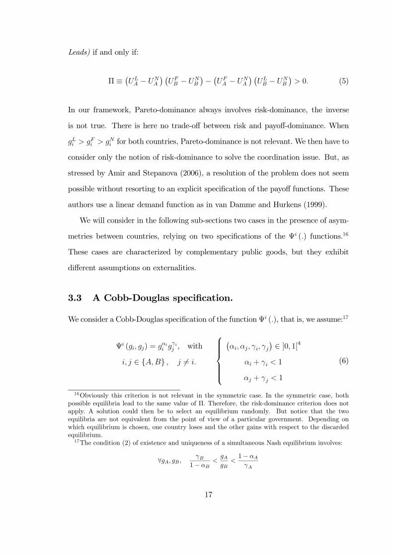
3.3 A Cobb-Douglas speciÞcation.
We consider a Cobb-Douglas speciÞcation of the function % ((), that is, we assume:17
% (&%% &') = &
(
% &) ' , with
!% ' " {#%"} % ' 6= !(
!!!!"
!!!!#
¡-%% -'% .%% .'
¢" ]0% 1[4
-% + .% * 1
-' + .' * 1
(6)
16Obviously this criterion is not relevant in the symmetric case. In the symmetric case, bothpossible equilibria lead to the same value of . Therefore, the risk-dominance criterion does notapply. A solution could then be to select an equilibrium randomly. But notice that the twoequilibria are not equivalent from the point of view of a particular government. Depending onwhich equilibrium is chosen, one country loses and the other gains with respect to the discardedequilibrium.
17The condition (2) of existence and uniqueness of a simultaneous Nash equilibrium involves:
#' ! '! !(!
1! )!*'
'!*1! ) (
17
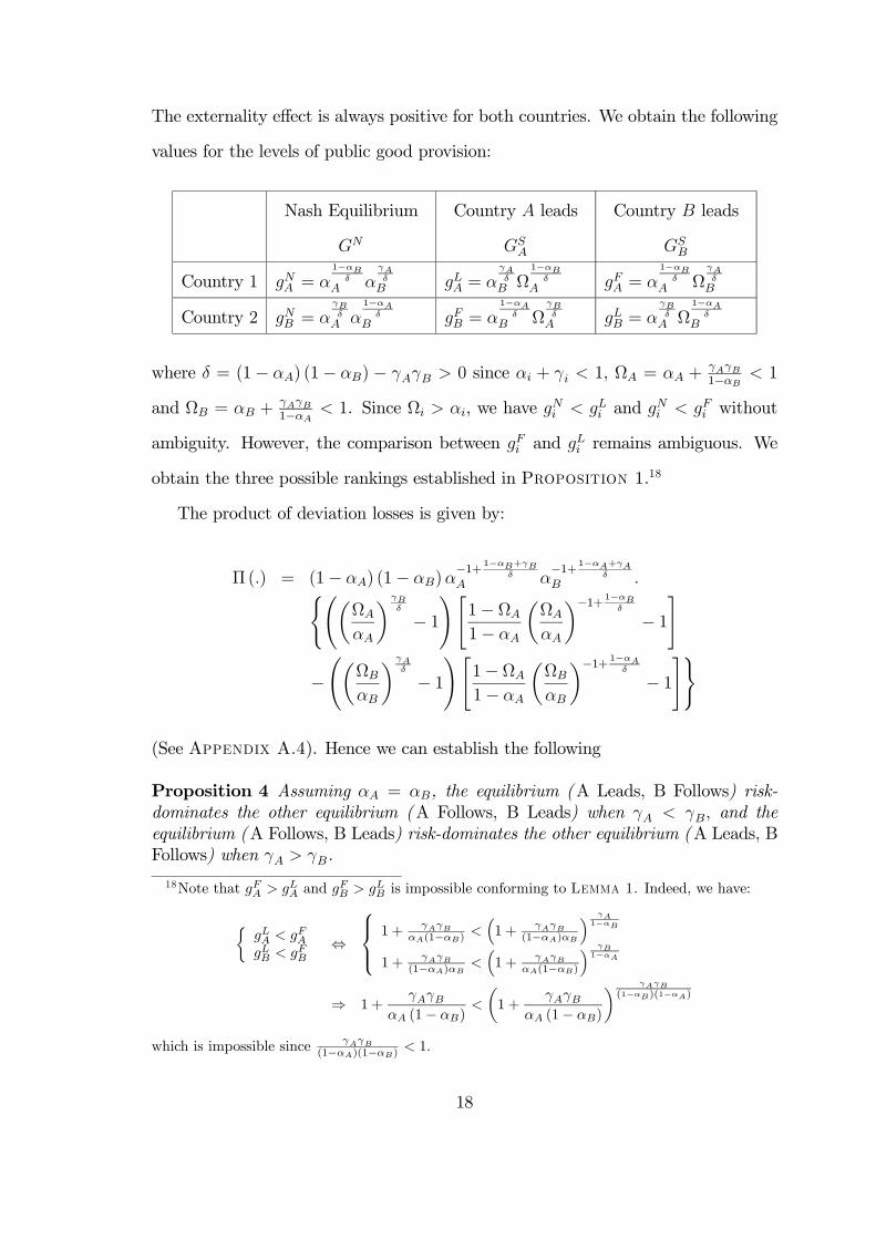
The externality e ect is always positive for both countries. We obtain the following
values for the levels of public good provision:
Nash Equilibrium
Country # leads
*!
Country " leads
*"
Country 1 & ! = -1 !"
#$"
! !" = #$"
!
1 !"
!# = 1 !"
#$"
!
Country 2 !$! = #!"
1 $"
! !#! = 1 $"
!
#!"
!"! = #!"
1 $"
!
where " = (1 ) (1 !) # #! $ 0 since % + #% % 1, = +&$&!1 '!
% 1
and ! = ! +&$&!1 '$
% 1. Since % $ %, we have !$% % !"% and !$% % !#% without
ambiguity. However, the comparison between !#% and !"% remains ambiguous. We
obtain the three possible rankings established in Proposition 1.18
The product of deviation losses is given by:
! (&) = (1 ) (1 !) 1+
1 !+#!"
1+
1 $+#$"
! &(õ
¶#!"
1
!"1 1
µ
¶ 1+
1 !"
1
#
õ !
!
¶#$"
1
!"1 1
µ !
!
¶ 1+
1 $"
1
#)
(See Appendix A.4). Hence we can establish the following
Proposition 4 Assuming = !, the equilibrium ( A Leads, B Follows) risk-dominates the other equilibrium ( A Follows, B Leads) when # % #!' and theequilibrium ( A Follows, B Leads) risk-dominates the other equilibrium ( A Leads, BFollows) when # $ #!.
18Note that ! ! "! and # ! "# is impossible conforming to Lemma 1. Indeed, we have:
½ "! " ! "# " #
!
!"
!#
1 + $ $!% (1 %!)
"
³1 + $ $!
(1 % )%!
´ " 1 #!
1 + $ $!(1 % )%!
"
³1 + $ $!
% (1 %!)
´ "!1 #
" 1 +#!##
$! (1 $#)"
µ1 +
#!##
$! (1 $#)
¶ " "!
(1 #!)(1 # )
which is impossible since $ $!(1 % )(1 %!)
" 1.
18
Proof. For = ! = , we have = ! = and then
! (&) = (1 )2 2+2 2 +!"+!#
$
"1
1
µ
¶ 1+1
$
1
#"µ
¶!#$
µ
¶!"$
#
Thus we have ! " !! involves ! (#) " 0#¤
Notice that +!" $ 1 involves %#" " %$" (& = '()). When !! $ ! ( the spillover
e ect is smaller from ) to ' than from ' to ): ) values more the foreign public
good than it is the case for '. Hence, ) has more interest in Follows than country '.
Both countries lose in case of simultaneous moves. Hence, since both players know
that ) is more interested in being the follower than ' and that a consistent choice
of moves delivers for both players positive advantages compared with the outcome of
disagreements over moves, the equilibrium is that ' chooses Leads and ) Follows.
) is able to push ' to assume leadership by selecting Follows and thus can extract
the second-mover advantage. The reverse explanation holds when !! " ! #
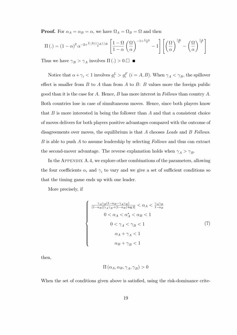
In the Appendix A.4, we explore other combinations of the parameters, allowing
the four coe!cients " and !" to vary and we give a set of su!cient conditions so
that the timing game ends up with one leader.
More precisely, if
!!!!!!!!!!"
!!!!!!!!!!#
%"%#(1 &# %"%#)(1 &#)[%"%#+(1 &#) log 2]
$ ! $%"%#1 &#
0 $ ! $ !! $ $ 1
0 $ !! $ ! $ 1
! + !! $ 1
+ ! $ 1
(7)
then,
! ( !( ( !!( ! ) " 0
When the set of conditions given above is satisÞed, using the risk-dominance crite-
19
rion, the outcome of the timing game is that ' leads and ) follows.
If the two relative coe!cients pondering the national public goods ( ! and )
are su!ciently distant ( ! $$ ), then the country with the lowest coe!cient, ',
emerges as the leader from the timing game. As a leader, by increasing its own level
compared to the Nash level19, it will trigger a larger increase in the other country’s
provision because of the complementarity assumption, which is beneÞcial to the
leader because of the positive externality e ect; on the other hand, if ) is a leader,
given that ' as a follower will not tend to act much, i.e. increase its provision
level (for opposite reasons), the gain of ' as a follower with respect to the Nash
solution, is not that large. The opposite reasoning explains why the country with
the largest coe!cient, ), has the more to lose from not being a follower. Since this
is understood by both players, ) chooses Follows and ' Leads.
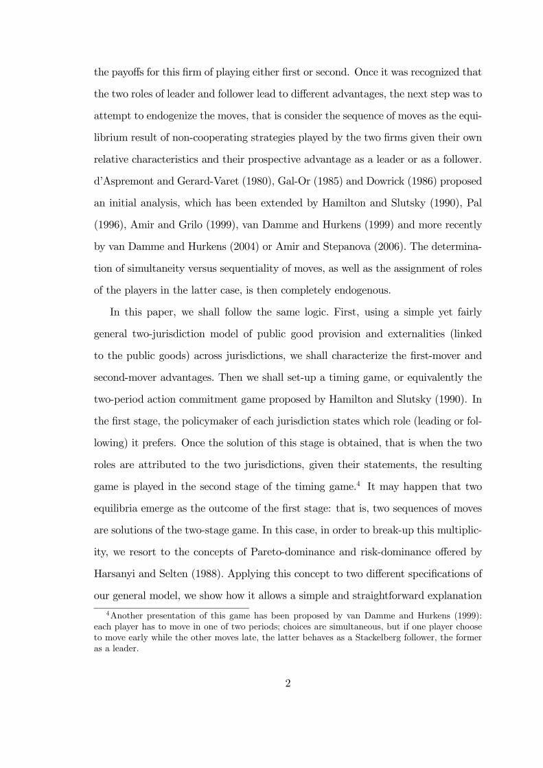
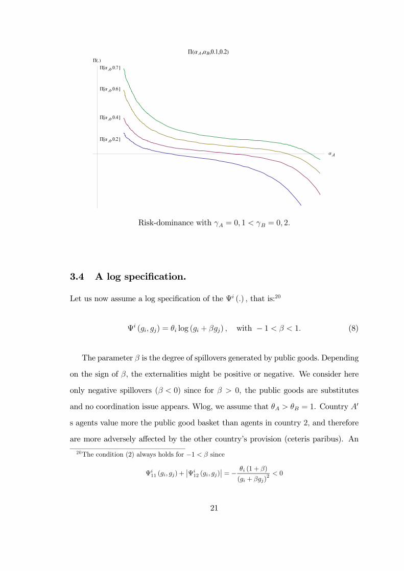
Resorting to simulations, we can also identify the roles assumed by the two
countries in the equilibrium of the timing game. The following graphic give some
illustrations of the function ! ( !( ( !!( ! ). When the curb is under the abscissa
axe, the risk-dominant equilibrium is the Stackelberg one where country ' follows.
19cf Proposition 1.
20
!A,0.2!
!A,0.4!
!A,0.6!
!A,0.7!
!A
".#
"!A,!B,0.1,0.2#
Risk-dominance with !! = 0( 1 $ ! = 0( 2#
3.4 A log speciÞcation.
Let us now assume a log speciÞcation of the "" (#) ( that is:20
"" (%"( %') = *" log (%" + +%') ( with 1 $ + $ 1# (8)
The parameter + is the degree of spillovers generated by public goods. Depending
on the sign of +, the externalities might be positive or negative. We consider here
only negative spillovers (+ $ 0) since for + " 0, the public goods are substitutes
and no coordination issue appears. Wlog, we assume that *! " * = 1. Country '0
s agents value more the public good basket than agents in country 2( and therefore
are more adversely a ected by the other country’s provision (ceteris paribus). An
20The condition (2) always holds for 1 ! since
11 ( ! !) +
¯̄
12 ( ! !)
¯̄=
" (1 + #)
( + # !)2 $ 0
21
exemple of such public goods is defense spending among rival countries: inhabitants
of country are more sensitive to their national security. The following table gives
the levels of public good in the di erent games.
Nash Equilibrium
!
Country leads
!!"
Country " leads
!!#
Country 1 # " =$ %
1 %2#&" = $"
%
1 %2#'" = $" +
%(%($ +%) 1)
1 %2
Country 2 # # =1 %$ 1 %2
#'# = 1 +%(% $ (1 %)2)
1 %2#&# = 1
%
1 %2$"
We deduce the following rankings of the level of the public goods, directly from
Proposition 1:
!% " ] 1& 0[ & # " ' #'" ' #
&"
!% "
¸ 1&
1
$"
& # # ' #
&# ' #
'#
!% "
¸ 1
$"& 0
& # # ' #
'# ' #
&#(
Let us denote by ($"& %) the di erence of the products given in (5):
($"& %) =%3
¡1 %2
¢2¡1 $2"
¢ ¡%2 +
¡1 %2
¢log¡1 %2
¢¢(
We then o er the following
Proposition 5 When (8) is assumed,(i) the equilibrium ( A Follows, B Leads) Risk-dominates ( A Leads, B Follows) for$" ' 1.(ii) this equilibrium is always Pareto-dominant for $" ' 1.
Proof. See Appendix A.5.¤
Playing Þrst is less risky for the country that values the less the basket of public
goods. This safer equilibrium in which country moves second is the neutral focal
point and, adopting the risk-dominance concept, the players will coordinate on it.
22
With the logarithm speciÞcation, we are able to establish that this equilibrium is also
Pareto-dominant. In other terms, country " always has a Þrst-mover advantage,
while country has a second-mover advantage.
Remark that the complementarity e ect is higher for country & as !"12(#& #) =
$"!#12(#& #)& as well as the negative externality e ect (in absolute values) as!"2 (#& #) =
$"!#2 (#& #)( As a follower, by decreasing its own level compared to the Nash level21,
it will trigger a larger decrease in "’s provision because of the lower complemen-
tarity e ect for ": this is beneÞcial to because of the negative externality e ect
(¡)'" )
"
¢large). On the other hand, if is a leader, given that " as a follower
and given the negative externality, the gain of as a leader with respect to the Nash
solution, is not that large (¡)&" )
"
¢small). This explains why the risk-dominance
e ect favors as a follower.
4 Conclusion.
The tools applied to study leadership in duopoly theory can be used to address
the relevance of leadership in public economics. Doing so in the matter of public
good provisions by two interdependent yet non-cooperating jurisdictions generates
neat and quite general results, which can easily be explained and may be applied
to various situations. Formally, leadership is equated to moving Þrst in a non-
cooperative game, that is being a Þrst-mover.
As a Þrst step, a positive comparison between the equilibrium levels obtained in
the simultaneous and sequential (non-simultaneous) games allows us to stress the
role of externalities and the nature of the interactions between the public goods in
the utility functions of the various agents (which are not assumed to be identical
across countries): whether they are complements or substitutes.
Then we can make explicit who beneÞts from a Þrst- or second-mover advantage
21using the formulas given above.
23
in the sequential game. This solely depends on the complementarity or substitutabil-
ity property of the public goods. As a result, it happens that being a leader is not
always beneÞcial but is so under certain circumstances only.
We are then able to tackle the issue of the existence and if any, the identity, of
a leader by means of a timing game. Again the complementarity or substitutability
property of the public goods plays a critical role. In particular, when public goods
are substitutes for all agents, then there is no leader. On the other hand, when
public goods are complements, the timing game generates two equilibria with each
country as a leader, respectively. We resort to the risk-dominance criterion to break
the tie in two cases with particular speciÞcations of the utility function, exhibiting
complementarity. On the whole, the results we obtain are strikingly simple yet
general, and easy to understand.
We provide a taxonomy of inter-jurisdictional interactions. Our results may be
used to reconsider the literature on political integration or centralization, where
the used benchmark is the simultaneous Nash equilibrium. When public goods
are complements, it could be argue that the relevant benchmark for assessing the
gains from centralization is not the simultaneous Nash equilibrium but a Stackelberg
equilibrium as the two countries may be better o with such a non-cooperative
equilibrium and may even resort to a timing game to select it.
As we have just said above, the tools that we have been using may be used to
study other issues in public economics. An immediate candidate which comes to
mind is the issue of tax competition either on production factors or on commodities.
One also can think of applying them in the context of international trade as well as
political economy problems.
It is also possible to relax the assumption of perfect information for both players
and adapt the notions we have just used to handle cases with imperfect informa-
24
tion.22 These issues are left for future research.
References
Alesina, A., I. Angeloni, and F. Etro (2005): “International Unions,” Amer-
ican Economic Review, 95(3), 602—615.
Amir, R., and I. Grilo (1999): “Stackelberg versus Cournot Equilibrium,” Games
and Economic Behavior, 26(1), 1—21.
Amir, R., and A. Stepanova (2006): “Second-mover advantage and price lead-
ership in Bertrand duopoly,” Games and Economic Behavior, 55(1), 1—20.
Bagwell, K., and A. Wolinsky (2002): “Game theory and industrial organiza-
tion,” in Handbook of Game Theory with Economic Applications, ed. by R. Au-
mann, and S. Hart, vol. 3 of Handbook of Game Theory with Economic Applica-
tions, chap. 49, pp. 1851—1895. Elsevier.
Barrett, S. (2007): Why Cooperate? The incentive to supply Global Public Goods.
Oxford University Press, Oxford, UK.
Batina, R. G., and T. Ihori (2005): Public Goods: Theories and Evidence.
Springer Verlag.
Bergstrom, T., L. Blume, and H. Varian (1986): “On the private provision of
public goods,” Journal of Public Economics, 29(1), 25—49.
Besley, T., and S. Coate (2003): “Centralized versus Decentralized Provision
of Local Public Goods: a Political Economy Approach,” Journal of Public Eco-
nomics, 87(12), 2611—2637.
22See Mailath (1993) and Daughety and Reinganum (1994).
25
Bloch, F., and U. Zenginobuz (2007): “The e ect of spillovers on the provision
of local public goods,” Review of Economic Design, 11(3), 199—216.
Cornes, R. (1993): “Dyke Maintenance and Other Stories: Some Neglected Types
of Public Goods,” The Quarterly Journal of Economics, 108(1), 259—271.
Cornes, R., and R. Hartley (2007): “Weak links, good shots and other public
good games: Building on BBV,” Journal of Public Economics, 91(9), 1684—1707.
d’Aspremont, C., and L.-A. Gerard-Varet (1980): “Stackelberg-Solvable
Games and Pre-Play Communication,” Journal of Economic Theory, 23(2), 201—
217.
Daughety, A. F., and J. F. Reinganum (1994): “Asymmetric Information Ac-
quisition and Behavior in Role Choice Models: An Endogenously Generated Sig-
naling Game,” International Economic Review, 35(4), 795—819.
Dowrick, S. (1986): “von Stackelberg and Cournot Duopoly: Choosing Roles,”
Rand Journal of Economics, 17(2), 251—260.
Dur, R. A., and H. J. Roelfsema (2005): “Why does Centralisation fail to
internalise Policy Externalities?,” Public Choice, 122(3-4), 395—416.
Ellingsen, T. (1998): “Externalities vs Internalities: a Model of Political Integra-
tion,” Journal of Public Economics, 68(2), 251—268.
Gal-Or, E. (1985): “First Mover and Second Mover Advantages,” International
Economic Review, 26(3), 649—653.
Hamilton, J. H., and S. M. Slutsky (1990): “Endogenous timing in duopoly
games: Stackelberg or Cournot equilibria,” Games and Economic Behavior, 2(1),
29—46.
26
Harsanyi, J. C., and R. Selten (1988): A General Theory of Equilibrium Selec-
tion in Games. MIT Press, Cambridge, MA.
Hirshleifer, J. (1983): “From Weakest-Link to Best-Shot: The Voluntary Provi-
sion of Public Goods,” Public Choice, 41(3), 371—386.
(1985): “From Weakest-Link to Best-Shot: Correction,” Public Choice,
46(2), 221—223.
Ihori, T. (2000): “Defense Expenditures and Allied Cooperation,” The Journal of
Conßict Resolution, 44(6), 854—867.
Kaul, I., I. Grunberg, and M. Stern (1999): Global Public Goods - Interna-
tional Cooperation in the 21st Century. Oxford University Press, New York.
Kempf, H., and E. Taugourdeau (2005): “Dépenses publiques dans une
économie à deux pays : Stackelberg versus Nash,” Annales d’Economie et de
Statistique, 77, 173—185.
Keohane, R. (1984): Robert Keohane, After Hegemony. Princeton University
Press, Princeton.
Lockwood, B. (2002): “Distributive Politics and the Cost of Centralization,”
Review of Economic Studies, 69(2), 313—337.
Mailath, G. J. (1993): “Endogenous Sequencing of Firm Decisions,” Journal of
Economic Theory, 59(1), 169—182.
Pahre, R. (1999): Leading Questions: How Hegemony A ects the International
Political Economy. University of Michigan Press, Michigan.
Pal, D. (1996): “Endogenous Stackelberg Equilibria with Identical Firms,” Games
and Economic Behavior, 12(1), 81—84.
27
Redoano, M., and K. A. Scharf (2004): “The Political Economy of Policy
Centralization: Direct versus Representative Democracy,” Journal of Public Eco-
nomics, 88(3-4), 799—817.
van Damme, E., and S. Hurkens (1999): “Endogenous Stackelberg Leadership,”
Games and Economic Behavior, 28(1), 105—129.
(2004): “Endogenous Price Leadership,” Games and Economic Behavior,
47(2), 404—420.
Varian, H. R. (1994): “Sequential contributions to public goods,” Journal of Public
Economics, 53(2), 165—186.
Vives, X. (1999): Olipoly Pricing. Old Ideas and New Tools. The MIT Press, Cam-
bridge, Massachusetts.
28
A Appendix
A.1 Proof of Proposition 1 (Comparison of the level ofpublic goods).
By deÞnitions of the Stackelberg and the Nash equilibria, we have
¡!! " !
"#
¡!! ¢¢>
¡!$ " !
$#
¢(9)
The leader of the Stackelberg game always has a utility level superior or equal to the utility levelobtained at the Nash equilibrium.
Moreover, we may establish from the FOCs at the Nash and Stackelberg equilibria that:
1
¡!" " !
!#
¢=
1
¡!$ " !
$#
¢= 1 (10)
We distinguish six cases depending on the signs of 2 (#) and
12 (#) for each country.
If 12 (#) $ 0, expression (10) then yields:
!" $ !$ !!# $ !$#!" % !$ !!# % !$#
(11)
If 12 (#) % 0, we have
!" $ !$ !!# % !$#!" % !$ !!# $ !$#
(12)
If 2 (#) $ 0, we have from the deÞnition of the Nash equilibrium:
¡!$ " !
$#
¢= argmax
%
¡! " !
$#
¢>
¡!! " !
$#
¢
The inequality !$# $ !"# then involves
¡!$ " !
$#
¢>
¡!! " !
$#
¢$
¡!! " !
"#
¢"
which contradicts the relation (9). We deduce that 2 (#) $ 0 !"# $ !$# .
In a similar way, if 2 (#) % 0, we deduce from the deÞnition of the Nash equilibrium that the
inequality !$# % !"# contradicts the relation (9), and we establish that 2 (#) % 0 !"# % !$# .
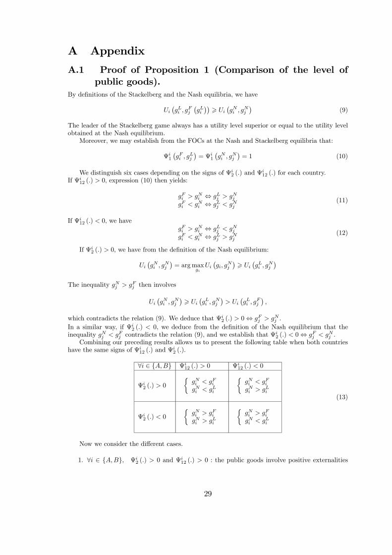
Combining our preceding results allows us to present the following table when both countrieshave the same signs of
12 (#) and 2 (#).
!& " {'"(} 12 (#) $ 0
12 (#) % 0
2 (#) $ 0
½!$ % !" !$ % !!
½!$ % !" !$ $ !!
2 (#) % 0
½!$ $ !" !$ $ !!
½!$ $ !" !$ % !!
(13)
Now we consider the di erent cases.
1. !& " {'"(}, 2 (#) $ 0 and
12 (#) $ 0 : the public goods involve positive externalities
29
and they are complements in both countries. We have:
#
12 (#)
11 (#)
#2 (#) $ 0 (14)
Combining the FOC for three di erent games and the sign of (14) yields
!& " {'"(} " 1
¡!! " !
"#
¢%
1
¡!" " !
!#
¢=
1
¡!$ " !
$#
¢(15)
From (15), we may establish that
!! % !" =$ !"# % !!# (16)
From Table (13) and (16), we deduce two following possible rankings:
½!! $ !" $ !$ !!# $ !"# $ !$#
or
½!! $ !" $ !$ !"# $ !!# $ !$#
(17)
We note that in the symmetric case only one possible ranking is possible:
!! $ !" $ !$
2. !& " {'"(}, 2 (#) % 0 and
12 (#) $ 0 : the public goods involve negative externalitiesand they are complements in both countries. We have:
#
12 (#)
11 (#)
#2 (#) % 0 (18)
Combining the FOC for three di erent games and the sign of (18) yields
!& " {'"(} " 1
¡!! " !
"#
¢$
1
¡!" " !
!#
¢=
1
¡!$ " !
$#
¢(19)
From (19), we have!! $ !" =$ !"# $ !!# (20)
From Table (13) and (20), we have two following rankings:
½!$ $ !" $ !! !$# $ !"# $ !!#
or
½!$ $ !! $ !" !$# $ !"# $ !!#
(21)
In the symmetric case, we have:!$ $ !" $ !!
3. !& " {'"(}, 2 (#) $ 0 and
12 (#) % 0 : the public goods involve positive externalitiesand they are substitutes in both countries. From Table (13), we have !"#& $ !$#& and then
!!#& % !$#& . We have also expression (18) and deduce the inequality (19). We then obtain:
!"# $ !!# =$ !! % !" . We obtain the following ranking:
½!" $ !$ $ !! !"# $ !$# $ !!#
(22)
In the symmetric case, we have:!" $ !$ $ !!
30
4. !& " {'"(}, 2 (#) % 0 and
12 (#) % 0 : the public goods involve negative externalities and
they are substitutes in both countries. From Table (13), we have !"#& % !$#& and !!#& $ !$#& .
We obtain expression (14) and thus inequality (15). We then have: !"# % !!# =$ !! $ !" .We deduce the following rankings
½!! $ !$ $ !" !!# $ !$# $ !"#
(23)
In the symmetric case, we have:!! $ !$ $ !"
5. !& " {'"(}, 2 (#) $ 0 and
12 (#) $ 0 $ #12 (#) : the public goods involve positive
externalities in both countries, but in contrast to the preceding case, they are complementsfor country & and substitutes in country ).
#
12 (#)
11 (#)
#2 (#) $ 0 and #
#12 (#)
#11 (#)
2 (#) % 0
We then have
1
¡!! " !
"#
¢$
1
¡!" " !
!#
¢=
1
¡!$ " !
$#
¢
#1
¡!!# " !
"
¢%
#1
¡!"# " !
!
¢= #
1
¡!$# " !
$
¢ (24)
Considering (11), (12) and the deÞnition of the Nash equilibrium, we know that !$ $ !" and !$# $ !"# contradict relation (9) for both countries. We then have: !$ % !" and
!$# % !"# . From expression (24), we deduce that:
!$ % !" !!# $ !$#!$# % !"# !! % !$
We can deduce that: !" $ !$ $ !! and min©!"# " !
!#
ª$ !$ hold. Moreover, from expres-
sion (24) we can establish that
!!# !"# =$ !! % !"
There are two possible rankings:
½!" $ !$ $ !! !!# $ !"# $ !$#
or
½!" $ !$ $ !! !"# $ !!# $ !$#
(25)
6. !& " {'"(}, 2 (#) % 0 and
12 (#) $ 0 $ #12 (#) : the public goods involve negative
externalities in both countries, but in contrast to the preceding case, they are complementsfor country & and substitutes in country ).
#
12 (#)
11 (#)
#2 (#) % 0 and #
#12 (#)
#11 (#)
2 (#) $ 0
We then have
1
¡!! " !
"#
¢%
1
¡!" " !
!#
¢=
1
¡!$ " !
$#
¢
#1
¡!!# " !
"
¢$
#1
¡!"# " !
!
¢= #
1
¡!$# " !
$
¢ (26)
Since  (#) % 0, we have !"#& % !$#& . From (26), we deduce that:
!" % !$ !!# $ !$#!"# % !$# !! $ !$
31
and!"# !
!# =$ !! $ !"
There are two possible rankings:
½!! $ !$ $ !" !$# $ !!# $ !"#
or
½!! $ !$ $ !" !$# $ !"# $ !!#
# (27)
¤
A.2 Proof of Proposition 2 (First-mover and second-moveradvantages).
We consider the three cases:
1. For !& " {'"(} " 12 (#) $ 0.
• If 2 (#) $ 0, the provision levels are given by (17). Using the deÞnition of the Þrst-
(second-) mover advantage, we get that, when !!# $ !"# "
¡!" " !
!#
¢>
¡!! " !
!#
¢$
¡!! " !
"#
¢"
where the Þrst inequality results from the deÞnition of the follower’s maximizationprogram and the second from the fact that !!# $ !"# and 2 (#) $ 0. Since !! $ !" always holds for at least one of the two countries in either one of the two possible rank-ings given by (17), we deduce that at least one country has a second-mover advantage.
• If 2 (#) % 0, we have the rankings given by (21). In a similar way as the precedingcase, we deduce that when !"# $ !!# "
¡!" " !
!#
¢>
¡!! " !
!#
¢$
¡!! " !
"#
¢"
where the Þrst inequality results from the deÞnition of the follower’s maximizationprogram and the second from the fact that !!# % !"# and 2 (#) % 0.
2. For !& " {'"(} " 12 (#) $ 0.
• If 2 (#) $ 0, we have the rankings (22). Since we have !$ &# $ !! &# , we establish that
¡!! " !
"#
¢>
¡!$ " !
$#
¢$
¡!" " !
$#
¢$
¡!" " !
!#
¢
where the Þrst inequality results from (9), the second from the deÞnition of the Nashmaximization program, and the third from the fact that !$# $ !!# and 2 (#) $ 0.Each country then has a Þrst-mover advantage.
• If 2 (#) % 0, we have the rankings (23). In a similar way as in the preceding case, we
establish that
¡!! " !
"#
¢>
¡!$ " !
$#
¢$
¡!" " !
$#
¢$
¡!" " !
!#
¢
where the Þrst inequality results from (9), the second from the deÞnition of the Nashmaximization program, and the third from the fact that !$# % !!# and 2 (#) % 0.Each country then has a Þrst-mover advantage.
32
3. 12 (#) $ 0 $
#12 (#).
• If 2 (#) $ 0" !& " {'"(}, we have the rankings (25). Since !$ $ !! always holds,
we establish that
#
¡!!# " !
"
¢> #
¡!$# " !
$
¢$ #
¡!"# " !
$
¢$ #
¡!"# " !
!
¢
Country ) then has a Þrst-mover advantage. When !!# $ !"# , we have
¡!" " !
!#
¢>
¡!! " !
!#
¢$
¡!! " !
"#
¢
Country & has a Þrst- (second-) mover advantage when !!# % ($)!"# .
• If 2 (#) % 0" !& " {'"(}, we have the rankings (27). Since !! $ !$ always holds,
we establish that
#
¡!!# " !
"
¢> #
¡!$# " !
$
¢$ #
¡!"# " !
$
¢$ #
¡!"# " !
!
¢"
which means that country ) has a Þrst-mover advantage. It may happen that country& also beneÞts from a Þrst-mover advantage, that is when the ranking !!# $ !"# obtains.
If !!# % !"# , then it beneÞts from a second-mover advantage. ¤
A.3 Proof of Proposition 3 (Subgame Perfect Equilibria).
From (9) we always have:
¡!! " !
"#
¢$
¡!$ " !
$#
¢, !& " {'"(}. In order to determine the
SPE, we only have to compare the utility levels when the country follows and when it playssimultaneously (
¡!" " !
!#
¢
¡!$ " !
$#
¢). We consider the six preceding cases:
1. !& " {'"(}, 12 (#) $ 0 :
• If 2 (#) $ 0, we have the rankings (17), and we establish that
¡!" " !
!#
¢>
¡!$ " !
!#
¢$
¡!$ " !
$#
¢"
where the Þrst inequality results from the deÞnition of the follower’s maximizationprogram and the second from the fact that !!# $ !$# and 2 (#) $ 0. We deduce thatthe SPE correspond to the two Stackelberg situations.
• If 2 (#) % 0" the rankings (21) yield
¡!" " !
!#
¢>
¡!$ " !
!#
¢$
¡!$ " !
$#
¢"
since !!# % !$# and 2 (#) % 0. As in the preceding case, the SPEs are the two
Stackelberg situations.
2. !& " {'"(}, 12 (#) % 0 :
• If 2 (#) $ 0, the ranking (22) yields
¡!$ " !
$#
¢>
¡!" " !
$#
¢$
¡!" " !
!#
¢"
where the Þrst inequality results from the deÞnition of the Bertrand-Nash maximiza-tion program and the second from the fact that !$# $ !!# and 2 (#) $ 0. We deducethat the SPE corresponds to the Bertrand-Nash situation (Leads is a strictly dominantstrategy for both countries).
33
• If 2 (#) % 0, the ranking (23) yields
¡!$ " !
$#
¢>
¡!" " !
$#
¢$
¡!" " !
!#
¢"
since !$# % !!# and 2 (#) % 0. We deduce that the SPE corresponds to the Bertrand-Nash situation.
3. 12 (#) $ 0 $
#12 (#).
• If  (#) $ 0, the rankings (25) yield
¡!" " !
!#
¢>
¡!$ " !
!#
¢$
¡!$ " !
$#
¢"
since !!# $ !$# and 2 (#) $ 0. We have also
#
¡!$# " !
$
¢> #
¡!"# " !
$
¢$ #
¡!"# " !
!
¢"
since !! % !$ and 2 (#) $ 0. Country ), the country for which public goods are
substitutes, has a strict dominant strategy (Leads). Country & always prefers to followthan to play the simultaneous game (
¡!" " !
!#
¢$
¡!$ " !
$#
¢). The SPE corre-
sponds to the situation where country ) leads and country & follows.
• If  (#) % 0, the rankings (27) yield
¡!" " !
!#
¢>
¡!$ " !
!#
¢$
¡!$ " !
$#
¢"
since !!# % !$# and 2 (#) % 0. We have also
#
¡!$# " !
$
¢> #
¡!"# " !
$
¢$ #
¡!"# " !
!
¢"
since !! $ !$ and 2 (#) $ 0. We have the same SPE as in the preceding case.
¤
A.4 Proof of Proposition 4.Using (6), after solving for the various games, we obtain:
$' = * + (1# +')+
1+1 !"
#
!"
! !
""! = # + !"
(1 !) 1+
1 #$"
! !
"# = # + $"
(1 ) 1+
1 #!"
!
"$! = # + (1 !) 1+
1 #$"
!
!"
!
"$ = # + (1 ) 1+
1 #!"
$"
! !
"#! = # + !"
(1 !) 1+
1 #$"
! $
34
and therefore:
¡"# "
"
¢ ¡"$! "
"!
¢= (1 !)
1+1 #$+ $
"
!
³
!"
!"
´
(1 )
1+1 #!
"
(1 ) 1+
1 #!"
¸
¡"$ "
"
¢ ¡"#! "
"!
¢= (1 )
1+1 #!+ !
"
³
$"
!
$"
!
´
(1 !)
1+1 #$
"
! (1 !) 1+
1 #$"
!
¸
where % = (1 ) (1 !) & &!, = +%$%!1 &!
' 1, ! = ! +%$%!1 &$
' 1.23
Applying the deÞnition of Harsanyi and Selten, the equilibrium where country ( follows ()!*)risk-dominates the other (*!) ) if and only if
! ( ! !! & ! &!) !¡"# "
"
¢ ¡"$! "
"!
¢ ¡"$ "
"
¢ ¡"#! "
"!
¢' 0
Using the preceding expression, it yields
! ( ! !! & ! &!) = (1 !) 1+
1 #$+ $"
!
³
!"
!"
´ (1 )
1+1 #!
"
(1 ) 1+
1 #!"
¸
(1 ) 1+
1 #!+ !"
³
$"
!
$"
!
´ (1 !)
1+1 #$
"
! (1 !) 1+
1 #$"
!
¸
Notice that
! (0! !! & ! &!) = (1 !) 1+
1 #$+ $"
!
³
!"
´ (1 )
1+1 #!
"
¸+ 0
For ! ! 6= 0, since 1 $1 &$
= 1 !1 &!
, expression ! ( ! !! & ! &!) becomes
! ($) = (1 ) (1 !) 1+
1 #!+ !"
1+
1 #$+ $"
!
!""""#
""""$
µ³ $
&$
´ !"
1
¶"1 $1 &$
³ $
&$
´ 1+ 1 #!"
1
#
µ³ !
&!
´ $"
1
¶"1 $1 &$
³ !
&!
´ 1+ 1 #$"
1
#
%""""&
""""'
For & ' &!, we have
! ( ! ! & ! &!) = (1 )2 2+
2 2#+ $+ !"
"1
1
µ
¶ 1+ 1 #"
1
#(µ
¶ !"
µ
¶ $"
)+ 0
Assuming ' ! involves the following inequalities
½ ' ! $
&$+ !
&!
Moreover we consider the situation where & ' &!, which yields³ $
&$
´ !"
+³ !
&!
´ $"
. We then
23>From ' + &' ' 1, we have %%1 &%
' 1 and then ( = ( +%%%&1 &%
' 1.
35
have
! ($) + (1 ) (1 !) 1+
1 #!+ !"
1+
1 #$+ $"
!
1 1
"µ !
!
¶ $"
1
#()µ
¶ 1+ 1 #!"
µ !
!
¶ 1+ 1 #$"
*
+
We focus on the sign of the last term. Since we face a transcendental expression, we can onlyestablish a su cient condition. We note that
,
,
(
)µ !
!
¶ 1+ 1 #$"
*
+ =µ !
!
¶ 2+ 1 #$"
(
)& &!%
!
!log
µ !
!
¶+
µ 1 +
1 %
¶ ,³ !
&!
´
,
*
+ + 0!
since !
&!+ 1 and )
)&$
³ !
&!
´= %$%!
(1 &$)2&!
+ 0. However, the sign of ))&$
"³ $
&$
´ 1+ 1 #!"
#is
ambiguous since ))&$
³ $
&$
´= %$%!
&2$(1 &!)' 0. We have:
,
,
(
)µ
¶ 1+ 1 #!"
*
+ =µ
¶ 2+ 1 #!"
(
) (1 !)2
%2
log
µ
¶+
µ 1 +
1 !%
¶ ,³ $
&$
´
,
*
+
We note that
" +& &!1 !
! log
µ
¶' log 2! (28)
which involves
,
,
(
)µ
¶ 1+ 1 #!"
*
+ '
µ
¶ 2+ 1 #!"
(
) (1 !)2
%2
log 2 +
µ 1 +
1 !%
¶ ,³ $
&$
´
,
*
+
Moreover, when respects the following condition
'& &! (1 ! & &!)
(1 !) [& &! + (1 !) log 2]! (29)
we have
(1 !)2
%2
log 2 +
µ 1 +
1 !%
¶ ,³ $
&$
´
, ' 0 =#
,
,
(
)µ
¶ 1+ 1 #!"
*
+ ' 0$
Under conditions (28) and (29), we establish that³ $
&$
´ 1+ 1 #!"
is decreasing in . Since ex-
pression³ !
&!
´ 1+ 1 #$"
is also increasing in , we deduce that:
If it exists ! $ [0! 1] such that
µ
!
¶ 1+ 1 #!"
=
µ !
!
¶ 1+ 1 #!$"
!
36
then the value of ! is unique under conditions (28) and (29). We obtain a third condition on :
' ! , (30)
which involves µ
¶ 1+ 1 #!"
+
µ !
!
¶ 1+ 1 #$"
Finally combining the di!erent preceding conditions and the assumptions on the others para-meters: ( !! & ! &!) $ [0! 1]
3, we obtain the following su cient set of conditions:
If !""""#
""""$
%$%!(1 &! %$%!)(1 &!)[%$%!+(1 &!) log 2]
' '%$%!1 &!
0 ' ' ! ' ! ' 10 ' & ' &! ' 1 + & ' 1 ! + &! ' 1
then,! ($) + 0
Notice that %$%!(1 &! %$%!)(1 &!)[%$%!+(1 &!) log 2]
' '%$%!1 &!
involves:
!#
$
'1+log 2
2
&! + & +1 log 2
2
! + 1 2%$%!1 log 2
¤
A.5 Proof of Proposition 5.• Risk-dominance:
It is obvious that ! (- !) " 0, ! # 0 and $ # 1 since (!2 +¡1! !2
¢log¡1! !2
¢) is
always negative on [!1 0].For $ # 1, (A Leads, B Follows) Risk-dominates (A Follows, B Leads).For $ " 1, (A Follows, B Leads) Risk-dominates (A Leads, B Follows).
• Pareto-dominance:We have:
%! ! %"
=!2 (! + $ )
1! !2+ $ log
¡1! !2
¢&
%"# ! %!
# = !!2 (1 + !$ )
1! !2! log
¡1! !2
¢&
which yield
$ " 0 %! # %"
$ " 1 " $ = !!2 +
¡1! !2
¢log¡1! !2
¢
!3 %"
# " %!# &
Country ' always has a second-mover-advantage, while country ( has a Þrst-mover advan-tage as soon as $ " 1. Thus, we have without ambiguity: the SPE (A Follows, B Leads)Pareto-dominates (A Leads, B Follows).¤
37