layer moduli of nebraska pavements for the new...

Nebraska Transportation Center

Report # MPM-08 Final Report

Layer Moduli of Nebraska Pavements for the New Mechanistic-Empirical Pavement Design Guide (MEPDG)

Yong-Rak Kim, Ph.D. Associate Professor Department of Civil Engineering University of Nebraska-Lincoln

“This report was funded in part through grant[s] from the Federal Highway Administration [and Federal Transit Administration], U.S. Department of Transportation. The views and opinions of the authors [or agency] expressed herein do not necessarily state or reflect those of the U. S. Department of Transportation.”

Nebraska Transportation Center262 WHIT2200 Vine StreetLincoln, NE 68583-0851(402) 472-1975

Soohyok ImGraduate Research Assistant

Hoki Ban, Ph.D. Postdoctoral Research Associate

26-1107-0108-001

2010

Layer Moduli of Nebraska Pavements for the New Mechanistic-Empirical Pavement

Design Guide (MEPDG)

Yong-Rak Kim, Ph.D. Hoki Ban, Ph.D.

Associate Professor Postdoctoral Research Associate

Department of Civil Engineering Department of Civil Engineering

University of Nebraska–Lincoln University of Nebraska–Lincoln

Soohyok Im

Graduate Research Assistant

Department of Civil Engineering

University of Nebraska–Lincoln

A Report on Research Sponsored by

Nebraska Transportation Center

University of Nebraska–Lincoln

Nebraska Department of Roads

December 2010

ii

Technical Report Documentation Page 1. Report No

MPM-08

2. Government Accession No. 3. Recipient’s Catalog No.

4. Title and Subtitle

Layer Moduli of Nebraska Pavements for the New Mechanistic-Empirical Pavement

Design Guide (MEPDG)

5. Report Date

December 2010

6. Performing Organization Code

7. Author/s

Soohyok Im, Yong-Rak Kim, and Hoki Ban

8. Performing Organization

Report No.

MPM-08

9. Performing Organization Name and Address

University of Nebraska-Lincoln (Department of Civil Engineering)

10. Work Unit No. (TRAIS)

362M Whittier Research Center

Lincoln, NE 68583-0856

11. Contract or Grant No.

26-1107-0108-001

12. Sponsoring Organization Name and Address

Nebraska Department of Roads (NDOR)

1400 Highway 2, PO Box 94759

Lincoln, NE 68509

13. Type of Report and Period

Covered

July 2007-December 2010

14. Sponsoring Agency Code

MATC TRB RiP No. 13602

15. Supplementary Notes

16. Abstract

As a step-wise implementation effort of the Mechanistic-Empirical Pavement Design Guide (MEPDG) for the design

and analysis of Nebraska flexible pavement systems, this research developed a database of layer moduli — dynamic

modulus, creep compliance, and resilient modulus — of various pavement materials used in Nebraska. The database

includes all three design input levels. Direct laboratory tests of the representative Nebraska pavement materials were

conducted for Level 1 design inputs, and surrogate methods, such as the use of Witczak’s predictive equations and the

use of default resilient moduli based on soil classification data, were evaluated to include Level 2 and/or Level 3 design

inputs. Test results and layer modulus values are summarized in the appendices. Modulus values characterized for each

design level were then put into the MEPDG software to investigate level-dependent performance sensitivity of typical

asphalt pavements. The MEPDG performance simulation results then revealed any insights into the applicability of

different modulus input levels for the design of typical Nebraska pavements. Significant results and findings are

presented in this report.

17. Key Words

MEPDG, Dynamic Modulus, Resilient

Modulus, Creep Compliance, Sensitivity

Analysis

18. Distribution Statement

19. Security Classification (of this report)

Unclassified

20. Security Classification (of this

page)

Unclassified

21. No. of

Pages

141

22. Price

iii

Table of Contents

Acknowledgments vi Disclaimer vii Abstract viii Chapter 1 Introduction 1

1.1 Research Objectives 2 1.2 Research Scope 3 1.3. Organization of the Report 4

Chapter 2 Background 5 2.1 MEPDG Analysis 5 2.2 MEPDG Inputs 6

2.2.1 Climatic Inputs 8 2.2.2 Traffic Inputs 8 2.2.3 Material Inputs 9

2.3 MEPDG Implementation Efforts 12 Chapter 3 Materials and Testing Facility 18

3.1 HMA Mixtures 18 3.2 Subgrade Soils 21 3.3 Testing Facility 23

Chapter 4 Laboratory Tests and Results 25 4.1 Tests and Results of Asphalt Materials 26

4.1.1 Binder Tests 26 4.1.2 Dynamic Modulus Test (AASHTO TP62) 27 4.1.3 Dynamic modulus characterization for Level 2 and Level 3 analysis 42 4.1.4 Creep compliance test (AASHTO T322) 55

4.2 Tests and Results of Subgrade Soils 74 4.2.1 Physical properties of unbound soils 74 4.2.2 Standard proctor test results of unbound soils 75 4.2.3 Resilient modulus test of unbound soils 77 4.2.4 Resilient modulus test results of unbound soils 81 4.2.5 Resilient modulus values for Level 2 MEPDG analysis 86 4.2.6 Resilient modulus values for Level 3 MEPDG analysis 87

Chapter 5 MEPDG Sensitivity Analysis 90 5.1 Sensitivity Analysis of Typical Pavement Structures 90

5.1.1 Design inputs for the sensitivity analysis 92 5.1.2 MEPDG simulations and results 93

Chapter 6 Summary and Conclusions 106 6.1 Conclusions 106 6.2 NDOR Implementation Plan 108

References 109 Appendix A HMA Database for MEPDG 113 Appendix B Soils Database for MEPDG 134

iv

List of Figures

Figure 2.1 MEPDG Design Procedure (NCHRP 1-37A 2004) ............................................6 Figure 2.2 Measured vs. Predicted Dynamic Modulus Curves (Flintsch et al. 2008) .........13

Figure 2.3 Measured Moduli Compared to Predicted Moduli (Kim et al. 2005) ................15 Figure 3.1 Project Locations of Collected HMA Mixtures..................................................19 Figure 3.2 Three Native Soils Selected for This Research ..................................................22 Figure 3.3 UTM-25kN Mechanical Test Station and Its Key Specifications ......................23 Figure 3.4 Testing Specimens with Associated Measuring Devices Installed ....................24

Figure 4.1 Specimen Production Process for the Dynamic Modulus Testing .....................28 Figure 4.2 Studs Fixing on the Surface of a Cylindrical Specimen .....................................30 Figure 4.3 A Specimen with LVDTs mounted in UTM-25kN Testing Station...................30

Figure 4.4 Typical Test Results of Dynamic Modulus Test ................................................31 Figure 4.5 Plot of Averaged Dynamic Moduli: SP4(0.5) NH281-4(119) Mixture .............34 Figure 4.6 Plot of Averaged Phase Angles: SP4(0.5) NH281-4(119) Mixture ...................34

Figure 4.7 Example of Developing a Master Curve and Its Shift Factors ...........................36 Figure 4.8 Master Curves of Each Mixture at a Reference Temperature (70°F) .................38

Figure 4.9 Master Curves of All Twenty HMA Mixtures at Different Input Levels...........45 Figure 4.10 Specimen Preparation Process for Creep Compliance Test .............................55 Figure 4.11 A Specimen with Extensometers Mounted in Testing Station .........................57

Figure 4.12 Creep Compliance at 14°F of All HMA Mixtures ...........................................60 Figure 4.13 Creep Compliance Results: Level 2 vs. Level 3...............................................64

Figure 4.14 Plots of Compaction Curves .............................................................................76

Figure 4.15 General Response of a Soil Specimen under Repeated Load...........................78

Figure 4.16 Confining Stress and Deviator Stress on a Triaxial Cylindrical Specimen ......79 Figure 4.17 Resilient Modulus Testing Setup (AASHTO T307) ........................................80

Figure 4.18 Specimens before and after Resilient Modulus Testing ...................................80 Figure 4.19 Resilient Modulus Test Results of Loess/Till Soil Specimen ..........................82 Figure 4.20 Predicted Moduli vs. Measure Moduli .............................................................84

Figure 5.1 FHWA Vehicle Classification ............................................................................91 Figure 5.2 Typical Full-Depth Asphalt Pavement Structures Used in Nebraska ................92

Figure 5.3 MEPDG Simulation Results of Longitudinal Cracking .....................................96 Figure 5.4 MEPDG Simulation Results of Alligator Cracking ...........................................98

Figure 5.5 MEPDG Simulation Results of Thermal Cracking ...........................................100

Figure 5.6 MEPDG Simulation Results of Surface Rutting ...............................................102

Figure 5.7 MEPDG Simulation Results of Total Rutting ...................................................103 Figure 5.8 MEPDG Simulation Results of IRI ...................................................................105

v

List of Tables

Table 2.1 Major Material Types for the MEPDG (AASHTO 2008) ...................................10 Table 2.2 Asphalt Materials and Their Test Protocols (AASHTO 2008) ............................11

Table 2.3 Summary of Implementation Efforts Pursued by Several State DOTs ...............12 Table 2.4 Summary of Sensitivity Analysis Results (Hoerner et al. 2007) .........................17 Table 3.1 Summary of Mixture Information........................................................................20 Table 3.2 Summary of Aggregate Gradation of Each Mixture ............................................21 Table 4.1 Various Tests of Asphalt Binder and Mixture for Each Input Level ...................25

Table 4.2 Various Tests of Soils and Unbound Materials for Each Input Level .................26 Table 4.3 Summary of Volumetric Characteristics of Specimens for Dynamic Modulus ..29 Table 4.4 Dynamic Moduli and Phase Angles of SP4(0.5) NH281-4(119) Mixture ..........33

Table 4.5 Sigmoidal Function Parameters and Shift Factors of All Mixtures .....................41 Table 4.6 Dynamic Modulus Estimation at Various Hierarchical Input Levels ..................42 Table 4.7 Air Voids, Gmb, and Gmm of Creep Compliance Testing Specimens ...................56

Table 4.8 Summary of Physical Property Tests and Results of Three Unbound Soils ........75 Table 4.9 Summary of Standard Proctor Test Results .........................................................77

Table 4.10 Combinations of Confining Pressure and Deviator Stress Applied ...................81 Table 4.11 Resulting Model Parameters and R

2-value of Each Soil....................................85

Table 4.12 Level 1 Resilient Modulus Model Parameters of Nine Stabilized Soils............85

Table 4.13 Models Relating Material Properties to MR (NCHRP 1-37A 2004) .................86 Table 4.14 Level 2 Resilient Modulus Value of Each Soil..................................................87

Table 4.15 Typical MR Values for Unbound Granular and Subgrade Materials .................88

Table 4.16 Level 3 Resilient Modulus Values Based on Group Classification ...................89

Table 5.1 Design Input Parameters for MEPDG Sensitivity Analysis ................................93 Table 5.2 Input Level Combinations Applied to Original Structures ..................................94

vi

Acknowledgments

The authors would like to thank the Nebraska Department of Roads (NDOR) for the

financial support needed to complete this study. In particular, the authors thank NDOR Technical

Advisory Committee (TAC) members for their invaluable comments.

vii

Disclaimer

This report was funded in part through grant(s) from the Federal Highway Administration

(and Federal Transit Administration), and the U.S. Department of Transportation. The views and

opinions of the authors (or agency) expressed herein do not necessarily state or reflect those of

the U. S. Department of Transportation.

viii

Abstract

As a step-wise implementation effort of the Mechanistic-Empirical Pavement Design

Guide (MEPDG) for the design and analysis of Nebraska flexible pavement systems, this

research developed a database of layer moduli — dynamic modulus, creep compliance, and

resilient modulus — of various pavement materials used in Nebraska. The database includes all

three design input levels. Direct laboratory tests of the representative Nebraska pavement

materials were conducted for Level 1 design inputs, and surrogate methods, such as the use of

Witczak’s predictive equations and the use of default resilient moduli based on soil

classification data, were evaluated to include Level 2 and/or Level 3 design inputs. Test results

and layer modulus values are summarized in the appendices. Modulus values characterized for

each design level were then put into the MEPDG software to investigate level-dependent

performance sensitivity of typical asphalt pavements. The MEPDG performance simulation

results then revealed any insights into the applicability of different modulus input levels for the

design of typical Nebraska pavements. Significant results and findings are presented in this

report.

1

Chapter 1 Introduction

A new Mechanistic-Empirical Pavement Design Guide (MEPDG) has been developed

and validated by many researchers and practitioners. The MEPDG was developed by the

National Cooperative Highway Research Program (NCHRP), under sponsorship of the American

Association of State Highway and Transportation Officials (AASHTO). The design guide

represents a challenging innovation to the way pavement design is performed; design inputs

include traffic (full load spectra for various axle configurations), material and subgrade

characterization, climatic factors, performance criteria, and many others. One of the most

interesting aspects of the design procedure is its hierarchical approach, i.e., the consideration of

different levels of inputs. Level 1 requires the engineer to obtain the most accurate design inputs

(e.g., direct testing of materials, on-site traffic load data, etc.). Level 2 requires testing, but the

use of correlations is allowed (e.g., subgrade modulus estimated through correlation with another

test), and Level 3 generally uses estimated values. Thus, Level 1 has the least possible error

associated with inputs, Level 2 uses estimated values or correlations, and Level 3 is based on the

default values.

Although evaluation of this new design procedure is still underway, many state

transportation agencies have already begun adaptation and local calibration of this procedure for

better and more efficient implementation of their local pavements. The Nebraska Department of

Roads (NDOR) has also initiated this implementation process for a new design for Nebraska

pavements, with a research project funded in 2006, MPM-04 “Toward Implementation of

Mechanistic-Empirical Pavement Design in Nebraska.” This project was primarily aimed at the

identification of the significant design factors involved and the development of a road map for a

step-by-step transition to the new design guide.

2

Among design factors involved in the new design guide, the key factors, from a materials

standpoint, include the layer moduli represented by dynamic modulus and creep compliance for

asphalt layers in flexible pavements and the resilient modulus for soils and unbound aggregate

layers. These all represent mandatory design inputs that serve as stiffness indicators of the

pavement system. Recent research has clearly emphasized the importance of accurate evaluation

of layer moduli, because these moduli significantly affect overall pavement performance and

they are typically quite dependent on local materials and regional environments. Evaluation of

layer moduli, therefore, is viewed as a primary and most urgent implementation step.

1.1 Research Objectives

The primary objective of this research was to develop a database by performing tests of

dynamic modulus, creep compliance, and resilient modulus in various pavement materials used

in Nebraska. In addition to the direct laboratory testing of the representative Nebraska pavement

materials for Level 1 design inputs in the modulus database, surrogate methods, such as the use

of Witczak’s predictive equations and the use of default resilient moduli based on Nebraska soil

classification data, were also evaluated to include Level 2 and/or Level 3 design inputs. This

allows investigation of their applicability for the design of pavements that are normally subject to

low traffic volume. Modulus values characterized for each design level were then put into the

MEPDG software to investigate level-dependent performance sensitivity of typical asphalt

pavements. Findings from this study can also be related and/or compared to other studies that

have already been conducted in other states, so that better and more reliable implementation of

the new design concept can be accomplished for Nebraska’s asphalt pavements.

3

1.2 Research Scope

To accomplish the objectives, four primary tasks were performed in this research. Task 1

consisted of a careful review of the recent literature related to MEPDG implementation, putting

particular emphasis on the development of a layer modulus database. The second task was to

establish mechanical testing facilities and analysis programs for the modulus characterization of

various pavement materials (asphalt mixtures and soils). The UTM-25kN mechanical testing

equipment at the University of Nebraska-Lincoln (UNL) geomaterials laboratory was used for

this effort, with several additions of testing accessories and new devices. The third task in this

research was the selection and laboratory testing of local materials and mixtures to identify layer

modulus characteristics that lead to the modulus database. The database includes all three design

input levels. Task 4 uses the layer modulus database to perform sensitivity analyses by MEPDG

simulations to investigate the effects of modulus input levels on overall pavement performance.

The MEPDG performance simulation results can then be used to search for any insights into the

applicability of different modulus input levels for the design of typical Nebraska pavements.

4

1.3. Organization of the Report

This report is composed of six chapters. Following this introduction (Chapter 1), Chapter

2 presents background information related to the new design guide, MEPDG and its local

implementation efforts, focusing in particular on the development of the modulus database.

Chapter 3 presents detailed descriptions of material selection and the testing facilities used in this

research. Chapter 4 shows the results of the laboratory tests conducted, which led to the MEPDG

design input database for each design level. The design input database is tabulated for individual

asphalt mixtures and soil samples and is located in the appendices. Chapter 5 provides a

discussion of sensitivity analyses of pavement performance conducted with different MEPDG

input levels. Finally, Chapter 6 provides a summary and conclusions of this study. NDOR

implementation plans are also presented in that chapter.

5

Chapter 2 Background

This chapter presents background information related to the new design guide, MEPDG,

and its local implementation efforts by other researchers. The discussion focuses in particular on

the development of the modulus database and its application to local practices to investigate

design input sensitivity.

2.1 MEPDG Analysis

The MEPDG is an analysis tool that enables prediction of pavement performances over

time for a given pavement structure subjected to variable conditions, such as traffic and climate.

The mechanistic-empirical design of the new and reconstructed flexible pavements requires an

iterative hands-on approach by the designer. The designer must select a trial design and then

analyze the design to determine if it meets the performance criteria established by the designer. If

the trial design does not satisfy the performance criteria, the design is modified and reanalyzed

until the design satisfies the performance criteria (NCHRP 1-37A 2004).

The procedure for use of the MEPDG depends heavily on the characterization of the

fundamental engineering properties of paving materials. It requires a number of input data in

four major categories: traffic, materials, environmental influences, and pavement response and

distress models. As shown in figure 2.1, the design procedure accounts for the environmental

conditions that may affect pavement response. These pavement responses were determined by

mechanistic procedures. The mechanistic method determined structural response (i.e., stresses

and strains) in the pavement structure. The transfer function was utilized for direct empirical

calculation of individual distresses such as top-down cracking, bottom-up cracking, thermal

cracking, rutting, and roughness.

6

Figure 2.1 MEPDG Design Procedure (NCHRP 1-37A 2004)

2.2 MEPDG Inputs

The MEPDG represents a challenging innovation in the way that pavement design is

performed; design inputs include traffic (full load spectra for various axle configurations),

material characterization, climatic factors, performance criteria, and many other factors. One of

the most interesting aspects of the design procedure is its hierarchical approach; that is, the

consideration of different levels of inputs. Level 1 requires the engineer to obtain the most

accurate design inputs (e.g., direct testing of materials, on-site traffic load data, etc.). Level 2

requires testing, but the use of correlations is allowed (e.g., subgrade modulus estimated through

correlation with another test). Level 3 generally uses estimated values. Thus, Level 1 has the

least possible error associated with inputs, Level 2 uses estimated values or correlations, and

Level 3 is based on the default values. This hierarchical approach enables the designer to select

the design input depending on the degree of significance of the project and the availability of

resources. The three levels of inputs are described as follows (NCHRP 1-37A 2004):

7

Level 1 input provides the highest level of accuracy and, accordingly, has the lowest level of

uncertainty or error. Level 1 design generally requires project-specific input, such as material

input measured by laboratory or field testing, site-specific axle load spectra data, or

nondestructive deflection testing. Because these types of inputs require additional time and

resources, Level 1 inputs are generally used for research, forensic studies, or projects in

which a low probability of failure is important.

Level 2 input supplies an intermediate level of accuracy that is closest to the typical

procedures used with earlier editions of the AASHTO guide. Level 2 input would most likely

be user-selected from an agency database, derived from a limited testing program, or

estimated through correlations. Examples of input include estimations of asphalt concrete

dynamic modulus from binder, aggregate, and mix properties; estimations of Portland cement

concrete elastic moduli from compressive strength tests; or use of site-specific traffic volume

and traffic classification data in conjunction with agency-specific axle load spectra. Level 2

input is most applicable for routine projects with no special degree of significance.

Level 3 input affords the lowest level of accuracy. This level might be used for designs

where the consequences of early failure are minimal, as with lower-volume roads. Inputs

typically would be user-selected values or typical averages for the region. Examples include

default unbound materials, resilient modulus values, or the default Portland cement concrete

coefficient of thermal expansion for a given mix class and aggregates used by an agency.

8

2.2.1 Climatic Inputs

In the 1993 AASHTO design guide, the climatic variables were handled with seasonal

adjustments and application of drainage coefficients. In the MEPDG, however, temperature

changes and moisture profiles in the pavement structure and subgrade over the design life of a

pavement are fully considered by using a sophisticated climatic modeling tool called the

Enhanced Integrated Climatic Model (EICM). The EICM model simulates changes in behavior

and characteristics of pavement and subgrade materials, in conjunction with climatic conditions,

over the design life of the pavement. To use this model, a relatively large number of input

parameters are needed as follows (NCHRP 1-37A 2004):

General information

Weather-related information

Groundwater table depth

Drainage and surface properties

Pavement structure materials

2.2.2 Traffic Inputs

For traffic analysis, the inputs for the MEPDG are much more complicated than are those

required by the 1993 AASHTO design guide. In the 1993 design guide, the primary traffic-

related input was the total design 80 kN equivalent single axle loads (ESALs) expected over the

design life of the pavement. In contrast, the more sophisticated traffic analysis in the MEPDG

uses axle load spectral data. The following traffic-related input is required for the MEPDG

(NCHRP 1-37A 2004):

Base year truck-traffic volume (the year used as the basis for design computation)

Vehicle (truck) operational speed

9

Truck-traffic directional and lane distribution factors

Vehicle (truck) class distribution

Axle load distribution factors

Axle and wheel base configurations

Tire characteristics and inflation pressure

Truck lateral distribution factors

Truck growth factors

2.2.3 Material Inputs

There are a number of material inputs for the design procedure and various types of test

protocols to measure material properties. Table 2.1 summarizes different types of materials

involved in the MEPDG, and table 2.2 shows the material properties of the hot mix asphalt

(HMA) layer and test protocols to characterize the HMA materials.

10

Table 2.1 Major Material Types for the MEPDG (AASHTO 2008)

Asphalt Materials

Stone Matrix Asphalt (SMA)

Hot Mix Asphalt (HMA)

o Dense Graded

o Open Graded Asphalt

o Asphalt Stabilized Base Mixes

o Sand Asphalt Mixtures

Cold Mix Asphalt

o Central Plant Processed

o In-Place Recycled

PCC Materials

Intact Slabs – PCC

o High Strength Mixes

o Lean Concrete Mixes

Fractured Slabs

o Crack/Seat

o Break/Seat

o Rubblized

Chemically Stabilized Materials

Cement Stabilized Aggregate

Soil Cement

Lime Cement Fly Ash

Lime Fly Ash

Lime Stabilized Soils

Open-graded Cement Stabilized Aggregate

Non-Stabilized Granular Base/Subbase

Granular Base/Subbase

Sandy Subbase

Cold Recycled Asphalt (used as

aggregate)

o RAP (includes millings)

o Pulverized In-Place

Cold Recycled Asphalt Pavement (HMA

plus aggregate base/subbase)

Sub-grade Soils

Gravelly Soils (A-1;A-2)

Sandy Soils

o Loose Sands (A-3)

o Dense Sands (A-3)

o Silty Sands (A-2-4;A-2-5)

o Clayey Sands (A-2-6; A-2-7)

Silty Soils (A-4;A-5)

Clayey Soils, Low Plasticity Clays (A-6)

o Dry-Hard

o Moist Stiff

o Wet/Sat-Soft

Clayey Soils, High Plasticity Clays

(A-7)

o Dry-Hard

o Moist Stiff

o Wet/Sat-Soft

Bedrock

Solid, Massive and Continuous

Highly Fractured, Weathered

11

Table 2.2 Asphalt Materials and Their Test Protocols (AASHTO 2008)

Design Type Measured Property Source of Data Recommended Test Protocol and/or

Data Source Test Estimate

New HMA (new

pavement and

overlay

mixtures), as

built properties

prior to opening

to truck traffic

Dynamic modulus X AASHTO TP 62

Tensile strength X AASHTO T 322

Creep Compliance X AASHTO T 322

Poisson’s ratio

X National test protocol unavailable.

Select MEPDG default relationship

Surface shortwave

absorptivity

X

National test protocol unavailable.

Use MEPDG default value.

Thermal conductivity X ASTM E 1952

Heat capacity X ASTM D 2766

Coefficient of thermal

contraction

X


Use MEPDG default values.

Effective asphalt content

by volume

X

AASHTO T 308

Air voids X AASHTO T 166

Aggregate specific gravity X AASHTO T 84 and T 85

Gradation X AASHTO T 27

Unit Weight X AASHTO T 166

Voids filled with asphalt

(VFA)

X

AASHTO T 209

Existing HMA

mixtures, in-

place properties

at time of

pavement

evaluation

FWD back-calculated

layer modulus

X

AASHTO T 256 and ASTM D 5858

Poisson’s ratio X


Use MEPDG default values.

Unit Weight X AASHTO T 166 (cores)

Asphalt content X AASHTO T 164 (cores)

Gradation

X AASHTO T 27 (cores or blocks)

Air voids X AASHTO T 209 (cores)

Asphalt recovery X AASHTO T 164/T 170/T 319 (cores)

Asphalt (new,

overlay, and

existing

mixtures)

Asphalt Performance

Grade (PG), OR

Asphalt binder complex

shear modulus (G*) and

phase angle (), OR

Penetration, OR

Ring and Ball Softening

Point

Absolute Viscosity

Kinematic Viscosity

Specific Gravity, OR

Brookfield Viscosity

X

X

X

X

X

AASHTO T 315

AASHTO T 49

AASHTO T 53

AASHTO T 202

AASHTO T 201

AASHTO T 228

AASHTO T 316

Note: The global calibration factors included in version 1.0 of the MEPDG software for HMA pavements were

determined using the NCHRP 1-37A viscosity based predictive model for dynamic modulus.

12

2.3 MEPDG Implementation Efforts

Table 2.3 summarizes some of the MEPDG implementation efforts attempted by several

state DOTs. As is evident from the table, most implementation studies were based on the

development of a layer modulus database for local pavement materials and mixtures as a first

step. Sensitivity or parametric analyses of design input variables related to local pavement

performance were also pursued. Sensitivity analysis can identify how each design input

parameter affects pavement performance.

Table 2.3 Summary of Implementation Efforts Pursued by Several State DOTs

Literature Research Purpose Significant Findings

Williams (2007)

- Evaluation of 21 HMA

mixtures

- Development of pavement

structures using the MEPDG

- Most of the predictive models of version 0.8

need further refinement.

Witczak and Bari

(2004)

- Development of database of

dynamic modulus for lime

modified asphalt mixtures

- Higher dynamic modulus from lime

modified HMA mixtures than unmodified

mixtures

- Recommendation of testing protocol-

Khazanovich et al.

(2006)

-Development of Level 1 and

Level 2 inputs

- Significant effect of thickness and stiffness

of the AC and base layers on the predicted

subgrade moduli

Coree et al. (2005)

- Investigation of sensitivity of

input parameters to

performance prediction

- Categorized the inputs for all distresses as

highly significant and significant and not

significant

- Identified critical factors affecting predicted

pavement performance from the MEPDG

Schwartz (2007)

Kesiraju et al.

(2007)

Velasquez et al.

(2009)

Fernando et al.

(2007)

Ali (2005)


input parameters to

performance prediction

- Identified critical factors affecting predicted

pavement performance from the MEPDG

Daniel and

Chehab. (2008)


predicted performance to

assumed PG grade using Level

1, 2, and 3

- Level 1 analysis is least conservative for the

structure and mixtures

McCracken et al.

(2008)

- Investigation of impact of

using different input levels on

pavement design

- Using different hierarchal levels for the

critical inputs can have an effect on the design

thickness

13

Flintsch et al. (2007, 2008) evaluated HMA characteristics based on the testing procedure

established by the MEPDG to support its practical implementation in Virginia. They examined

the dynamic modulus, creep compliance, and tensile strength of eleven HMA mixtures produced

with PG 64-22 binder from different plants across Virginia. Test results indicated that Level 1

design inputs are necessary for HMA pavement projects with high significance, whereas Level 2

design could be used for design of pavements where low or medium traffic volumes are expected.

The predicted HMA moduli obtained from the Level 2 approach were relatively close to the

Level 1 measured values, as shown in figure 2.2. A ratio of the predicted to measured dynamic

modulus values varied between 0.5 and 0.9.

Figure 2.2 Measured vs. Predicted Dynamic Modulus Curves (Flintsch et al. 2008)

In 2005, Kim et al. conducted an experimental study on the dynamic modulus testing of

typical North Carolina HMA mixtures in two different testing modes: uniaxial compression and

14

indirect tension (IDT). The study included 42 HMA mixtures with varying aggregate sources,

aggregate gradations, asphalt sources, asphalt grades, and asphalt contents. This research found

that the binder variables (i.e., the source, performance grade, and content) have a much more

significant effect on the dynamic modulus than do the aggregate variables (i.e., source and

gradation). They also compared the dynamic modulus database (Level 1) developed from the

uniaxial compression testing mode to predicted values by using two dynamic modulus predictive

models: Witczak’s equation (Level 2 implemented in the MEPDG) and another

phenomenological model, the Hirsch model. Figure 2.3 illustrates a relatively good prediction

using Witczak’s model in the (a) and (b) graphs, whereas the (c) and (d) graphs show a mixture

with a relatively poor prediction. It appeared that Witczak’s prediction was more accurate at

cooler temperatures than at warmer temperatures. The Hirsch model, as shown in figure 2.3(b),

performed very poorly at 10°C and approximately the same as Witczak’s model at the remaining

temperatures. The poorer prediction of the Hirsch model at 10°C could be due to the fact that the

binder data at this temperature were extrapolated.

15

Figure 2.3 Measured Moduli Compared to Predicted Moduli (Kim et al. 2005)

Tashman et al. (2007) developed a database of dynamic modulus values of typical

Superpave HMA mixes that were widely used in the state of Washington. The database was used

to investigate the sensitivity of the dynamic modulus to HMA mix properties. They compared

performance predictions by the MEPDG with field performance data and reported that the

MEPDG over-predicted the longitudinal cracking compared to field performance data, and Level

3 analysis predicted distresses higher than Level 1 distresses. Richardson et al. (2009) evaluated

the resilient moduli for common Missouri subgrade soils and typical unbound granular base

materials. Their testing program included 27 common subgrade soils and five unbound granular

base materials. The tests were performed at their optimum water content and at elevated water

content. They concluded that the material source and fines content were highly significant for the

level of attained resilient modulus.

16

A similar study was conducted by Nazzal et al. (2008) to develop a database of resilient

modulus values of subgrade soils commonly used in Louisiana at different moisture content

levels. They also developed resilient modulus prediction models for Louisiana subgrade soils and

found a good agreement between the measured resilient modulus coefficient values and those

predicted using the developed regression models. They reported a significant difference between

the measured resilient modulus values of A-4 and A-6 soils and those recommended by the

MEPDG.

As mentioned earlier, sensitivity analysis of design input parameters can identify

important input parameters that significantly affect pavement performance among the entire

design inputs. Therefore, sensitivity analysis of design input parameters is considered an

important task that should be performed before implementing the new design guide into actual

practice. This is because the analysis results can provide useful and relevant information for

pavement design engineers in determining their appropriate level of effort for each design input.

Hoerner et al. (2007) selected inputs associated with five typical types of South Dakota

asphaltic pavements for sensitivity analyses. A total of 56 MEPDG simulations for new asphalt

pavement design were conducted with two representative climatic conditions. They ranked

design inputs in order of their significance to the pavement performance. Table 2.4 presents

sensitivity analysis results demonstrating design input parameters that are the most significantly

related to each performance indicator (i.e., longitudinal cracking, alligator cracking, and total

rutting).

17

Table 2.4 Summary of Sensitivity Analysis Results (Hoerner et al. 2007)

Input Parameter/Predictor

Rankings for Individual Performance Indicators Overall Order

of

Significance Longitudinal

Cracking

Alligator

Cracking

Total

Rutting

Average annual daily truck traffic 2 1 1 1

AC layer thickness 1 3 2 2

AC binder grade 4 2 5 3

Base resilient modulus 3 4 6 4

Subgrade resilient modulus 9 6 3 5

Traffic growth rate 6 5 8 6

Base layer thickness 5 8 10 7

Climate location 10 7 7 8

Tire Pressure 7 9 9 9

Depth of water table 12 14 4 10

Vehicle class distribution 8 10 13 11

AC mix gradation 11 11 12 12

AC creep compliance 13 12 14 13

Base plasticity index 15 15 11 14

Coef. of thermal contraction 14 13 15 15

Subgrade type 16 16 16 16

Truck hourly distribution factors 17 17 17 17

* Note: shaded cells indicate those variables found to be insignificant

18

Chapter 3 Materials and Testing Facility

This chapter presents the local materials and mixtures selected for this research. A total

of 20 hot mix asphalt (HMA) mixtures paved during 2008 and 2009 were collected from asphalt

field projects, and three unbound soils (loess, loess/till, and sandy silt) typically used for

roadway foundations in Nebraska pavements were obtained to characterize their physical

properties and resilient moduli. In addition to the testing of the three unbound soils, nine

stabilized soils (loess, till, and shale stabilized with hydrated lime, fly ash and cement kiln dust)

that had been tested by Hensley et al. (2007) for a previous NDOR research project were also

analyzed for their resilient modulus characteristics.

One of the major milestones planned for this research was to develop a mechanical

testing system to perform various modulus (stiffness) tests of different paving materials. The

UNL research team installed and used the UTM-25kN (Universal Testing Machine with a 25kN

load cell) mechanical testing station and related devices in the UNL geomaterials laboratory for

various mechanical tests of asphalt mixtures. The current UTM-25kN mechanical testing-

analysis facility was used for this study, but some improvements were necessary, such as an

installation of a triaxial cell with associated measuring devices to evaluate stress-dependent

modulus characteristics of soils.

3.1 HMA Mixtures

Based on the literature reviews and discussions with NDOR Technical Advisory

Committee (TAC) members, two major issues were considered for the testing of asphalt

mixtures: 1) the number of mixture types; and 2) the combination of materials of each mixture

type. In this research, 20 HMA mixtures from field projects were collected for two years: 2008 to

2009. Figure 3.1 shows the location where each HMA mixture was collected. As seen in the

19

figure, five different types of HMA mixtures (i.e., HRB, SPL, SP4(0.375), SP4(0.5), and SP5)

among 11 existing HMA mixture types (SPS, SPL, SP1 to SP6, SP4 Special, RLC, and LC) were

the focus of this study, since they are the primary types used for Nebraska asphalt pavements.

For each type of mixture, four field projects were collected, which resulted in a total of 20 HMA

mixtures.

HRB

SPL

SP4 (0.375)

SP4 (0.5)

SP5 (0.5)

Figure 3.1 Project Locations of Collected HMA Mixtures

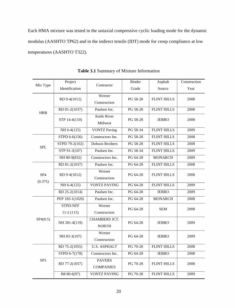
Table 3.1 summarizes mixture information such as project identification, contractor,

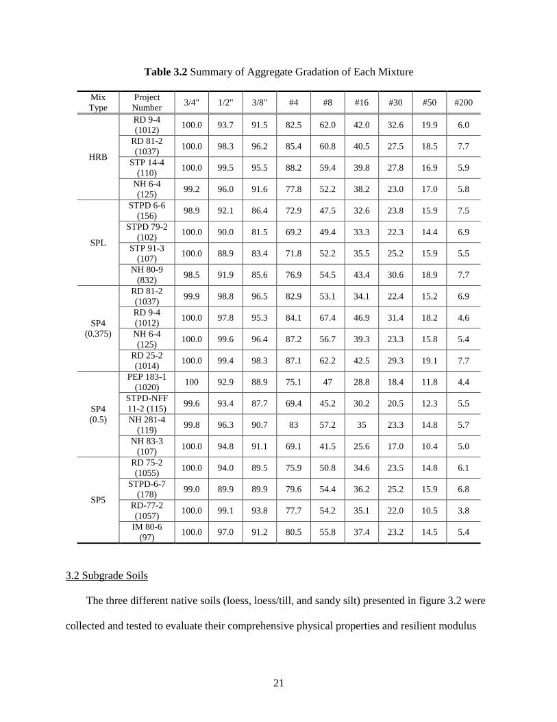
binder grade and source of each mixture, and construction year. Table 3.2 summarizes the

aggregate gradation of each mixture. The gradation values are crucial information for conducting

MEPDG analysis, such as predicting dynamic modulus characteristics of HMA mixtures for

Level 2 or Level 3 pavement design.

20

Each HMA mixture was tested in the uniaxial compressive cyclic loading mode for the dynamic

modulus (AASHTO TP62) and in the indirect tensile (IDT) mode for creep compliance at low

temperatures (AASHTO T322).

Table 3.1 Summary of Mixture Information

Mix Type Project

Identification Contractor

Binder

Grade

Asphalt

Source

Construction

Year

HRB

RD 9-4(1012) Werner

Construction PG 58-28 FLINT HILLS 2008

RD 81-2(1037) Paulsen Inc. PG 58-28 FLINT HILLS 2008

STP 14-4(110) Knife River

Midwest PG 58-28 JEBRO 2008

NH 6-4(125) VONTZ Paving PG 58-34 FLINT HILLS 2009

SPL

STPD 6-6(156) Constructors Inc. PG 58-28 FLINT HILLS 2008

STPD 79-2(102) Dobson Brothers PG 58-28 FLINT HILLS 2008

STP 91-3(107) Paulsen Inc. PG 58-34 FLINT HILLS 2009

NH 80-9(832) Constructors Inc. PG 64-28 MONARCH 2009

SP4

(0.375)

RD 81-2(1037) Paulsen Inc. PG 64-28 FLINT HILLS 2008

RD 9-4(1012) Werner

Construction PG 64-28 FLINT HILLS 2008

NH 6-4(125) VONTZ PAVING PG 64-28 FLINT HILLS 2009

RD 25-2(1014) Paulsen Inc. PG 64-28 JEBRO 2009

SP4(0.5)

PEP 183-1(1020) Paulsen Inc. PG 64-28 MONARCH 2008

STPD-NFF

11-2 (115)

Werner

Construction PG 64-28 SEM 2008

NH 281-4(119) CHAMBERS JCT.

NORTH PG 64-28 JEBRO 2009

NH 83-3(107) Werner

Construction PG 64-28 JEBRO 2009

SP5

RD 75-2(1055) U.S. ASPHALT PG 70-28 FLINT HILLS 2008

STPD 6-7(178) Constructors Inc. PG 64-28 JEBRO 2008

RD 77-2(1057) PAVERS

COMPANIES PG 70-28 FLINT HILLS 2008

IM 80-6(97) VONTZ PAVING PG 70-28 FLINT HILLS 2009

21

Table 3.2 Summary of Aggregate Gradation of Each Mixture

Mix

Type

Project

Number 3/4" 1/2" 3/8" #4 #8 #16 #30 #50 #200

HRB

RD 9-4

(1012) 100.0 93.7 91.5 82.5 62.0 42.0 32.6 19.9 6.0

RD 81-2

(1037) 100.0 98.3 96.2 85.4 60.8 40.5 27.5 18.5 7.7

STP 14-4

(110) 100.0 99.5 95.5 88.2 59.4 39.8 27.8 16.9 5.9

NH 6-4

(125) 99.2 96.0 91.6 77.8 52.2 38.2 23.0 17.0 5.8

SPL

STPD 6-6

(156) 98.9 92.1 86.4 72.9 47.5 32.6 23.8 15.9 7.5

STPD 79-2

(102) 100.0 90.0 81.5 69.2 49.4 33.3 22.3 14.4 6.9

STP 91-3

(107) 100.0 88.9 83.4 71.8 52.2 35.5 25.2 15.9 5.5

NH 80-9

(832) 98.5 91.9 85.6 76.9 54.5 43.4 30.6 18.9 7.7

SP4

(0.375)

RD 81-2

(1037) 99.9 98.8 96.5 82.9 53.1 34.1 22.4 15.2 6.9

RD 9-4

(1012) 100.0 97.8 95.3 84.1 67.4 46.9 31.4 18.2 4.6

NH 6-4

(125) 100.0 99.6 96.4 87.2 56.7 39.3 23.3 15.8 5.4

RD 25-2

(1014) 100.0 99.4 98.3 87.1 62.2 42.5 29.3 19.1 7.7

SP4

(0.5)

PEP 183-1

(1020) 100 92.9 88.9 75.1 47 28.8 18.4 11.8 4.4

STPD-NFF

11-2 (115) 99.6 93.4 87.7 69.4 45.2 30.2 20.5 12.3 5.5

NH 281-4

(119) 99.8 96.3 90.7 83 57.2 35 23.3 14.8 5.7

NH 83-3

(107) 100.0 94.8 91.1 69.1 41.5 25.6 17.0 10.4 5.0

SP5

RD 75-2

(1055) 100.0 94.0 89.5 75.9 50.8 34.6 23.5 14.8 6.1

STPD-6-7

(178) 99.0 89.9 89.9 79.6 54.4 36.2 25.2 15.9 6.8

RD-77-2

(1057) 100.0 99.1 93.8 77.7 54.2 35.1 22.0 10.5 3.8

IM 80-6

(97) 100.0 97.0 91.2 80.5 55.8 37.4 23.2 14.5 5.4

3.2 Subgrade Soils

The three different native soils (loess, loess/till, and sandy silt) presented in figure 3.2 were

collected and tested to evaluate their comprehensive physical properties and resilient modulus

22

characteristics. Based on discussions with NDOR TAC members, the three soils are considered

representative subgrade materials often used in Nebraska pavements. In order to characterize

physical properties of the soils, various laboratory tests were performed, including the specific

gravity test (AASHTO T100), Atterberg limit tests (AASHTO T89, T90), sieve analysis

(AASHTO T88), and hydrometer analysis (ASTM D422). For mechanical characterization of the

soils, the resilient modulus test designated in AASHTO T307 was performed with soil specimens

that were compacted at the maximum dry unit weight with an optimum moisture content, which

was pre-determined from a standard proctor test (AASHTO T99).

Figure 3.2 Three Native Soils Selected for This Research

In addition to the comprehensive testing of the three unbound native soils, nine stabilized

soils (loess, till, and shale stabilized with hydrated lime, fly ash and cement kiln dust,

respectively), which had been studied by Hensley et al. (2007) for a previous NDOR research

project, were also analyzed for their resilient modulus characteristics. This analysis was

attempted in order to provide a more general and comprehensive resilient modulus database of

the subgrade soils that are often stabilized with cementing agents in various pavement projects.

Sandy Silt (SS) Soil

Loess/Till (LT) Soil

Loess (L) Soil

23

Hensley et al. (2007) reported resilient modulus test results of the nine soils that were compacted

with an optimum amount of different types of pozzolans.

3.3 Testing Facility

All three layer modulus tests (i.e., the dynamic modulus test and creep compliance test

for HMA mixtures and the resilient modulus test for soils) were conducted using the UTM-25kN

mechanical test station. This equipment is capable of applying loads up to 25 kN static or 20 kN

dynamic over a wide range of loading frequencies. An environmental chamber is incorporated

with the loading frame, as presented in figure 3.3, to control testing temperatures. The chamber

can control temperatures ranging from 5ºF to 140ºF. Improved achievement of the target testing

temperatures of specimens was obtained by using a dummy specimen with a thermocouple

embedded in the middle of the specimen, as presented in the figure. Figure 3.3 also presents

other key features and specifications of the UTM-25kN test station.

Figure 3.3 UTM-25kN Mechanical Test Station and Its Key Specifications

Specifications

24

Figure 3.4(a) presents a cylindrical specimen (100 mm in diameter and 150 mm high)

with three linear variable differential transducers (LVDTs) attached on the surface to measure

vertical linear deformations in the uniaxial compressive cyclic loading mode for the dynamic

modulus test of HMA mixtures. In order to conduct the creep compliance test of HMA mixtures

at low temperature, two cross extensometers were attached to both faces of the indirect tensile

specimen, as shown in figure 3.4(b). In order to perform the resilient modulus test of soil

specimens, a universal triaxial cell with associated measuring devices was developed to evaluate

stiffness characteristics of subgrade soils that are stress-dependent. Figure 3.4(c) presents the

triaxial testing system.

(a) (b) (c)

Figure 3.4 Testing Specimens with Associated Measuring Devices Installed

25

Chapter 4 Laboratory Tests and Results

This chapter describes laboratory tests conducted for this study and presents the results.

Determination of layer stiffness characteristics of HMA mixtures for each MEPDG design level

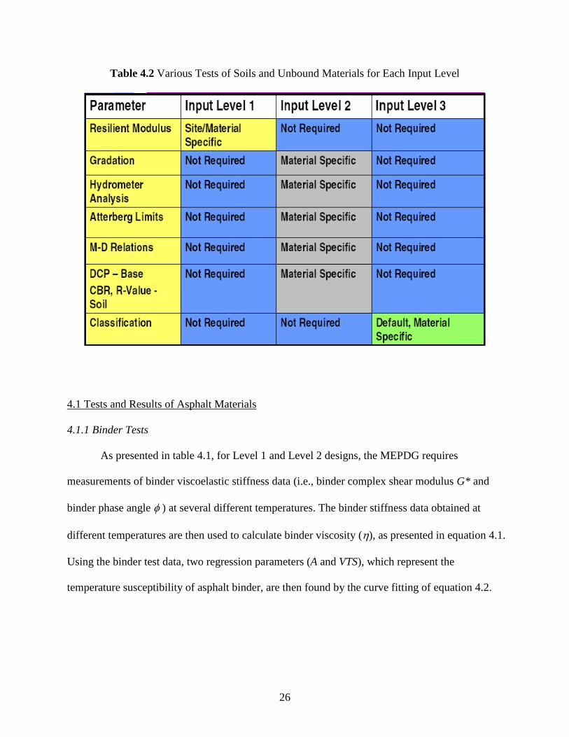
requires various tests of asphalt binder and HMA mixture, as summarized in table 4.1. Similarly,

table 4.2 presents soil laboratory tests necessary to perform each level of MEPDG design. As

previously mentioned, the triaxial resilient modulus test was conducted for Level 1, whereas

basic physical properties of soils, such as specific gravity, Atterberg limits, and gradations, were

identified for Level 2 or 3 inputs. Test results obtained from individual asphalt mixtures and soil

samples were then tabulated in the form of an MEPDG design input database and are presented

in the appendices.

Table 4.1 Various Tests of Asphalt Binder and Mixture for Each Input Level

26

Table 4.2 Various Tests of Soils and Unbound Materials for Each Input Level

4.1 Tests and Results of Asphalt Materials

4.1.1 Binder Tests

As presented in table 4.1, for Level 1 and Level 2 designs, the MEPDG requires

measurements of binder viscoelastic stiffness data (i.e., binder complex shear modulus G* and

binder phase angle ) at several different temperatures. The binder stiffness data obtained at

different temperatures are then used to calculate binder viscosity (), as presented in equation 4.1.

Using the binder test data, two regression parameters (A and VTS), which represent the

temperature susceptibility of asphalt binder, are then found by the curve fitting of equation 4.2.

27

8628.4*

sin

1

10

G (4.1)

RTVTSA logloglog (4.2)

where G* = asphalt binder complex shear modulus (Pa),

= asphalt binder phase angle (degree),

η = viscosity of asphalt binder (centi poise),

TR = temperature (Rankine) at which the viscosity was estimated, and

A and VTS = regression parameters.

Binders were evaluated with a dynamic shear rheometer (DSR) in oscillatory shear

loading mode using parallel plate test geometry. The DSR binder testing was performed at three

different temperatures (70ºF, 85ºF, and 100ºF). Binder test results and the two corresponding

regression parameters (A and VTS) for each HMA mixture are summarized in Appendix A. For

Level 3 MEPDG analysis, no testing was required for the two parameters. Default values of A

and VTS embedded in the MEPDG software are generated when one specifies the grade (either

traditional or Superpave performance) of the binder (NCHRP 1-37A 2004).

4.1.2 Dynamic Modulus Test (AASHTO TP62)

The dynamic modulus test is a linear viscoelastic test for asphalt concrete. The dynamic

modulus is an important input when evaluating pavement performance related to the temperature

and speed of traffic loading. The loading level for the testing was carefully adjusted until the

specimen deformation was between 50 and 75 microstrain, a level that is considered unlikely to

cause nonlinear damage to the specimen, so that the dynamic modulus would represent the intact

stiffness of the asphalt concrete.

28

A Superpave gyratory compactor was used to produce cylindrical samples with a

diameter of 150 mm and a height of 170 mm. The samples were then cored and cut to produce

cylindrical specimens with a diameter of 100 mm and a height of 150 mm. The target air void of

the cored and cut specimens was 4% ± 0.5%. Figure 4.1 demonstrates the specimen production

process using the Superpave gyratory compactor, core, and saw machines, and the resulting

cylindrical specimen used to conduct the dynamic modulus test.

Figure 4.1 Specimen Production Process for the Dynamic Modulus Testing

Table 4.3 summarizes air voids, bulk specific gravity (Gmb), maximum specific gravity

(Gmm), asphalt content, and compaction temperature of each dynamic modulus testing specimen.

As shown in the table, two specimens were tested for each mixture. It should also be noted that

the volumetric characteristics presented in the table are used to provide necessary model inputs,

such as effective binder content (%), air voids (%), and total unit weight, for MEPDG analysis.

The model inputs that are related to the mixture volumetric properties are summarized in

Appendix A.

29

Table 4.3 Summary of Volumetric Characteristics of Specimens for Dynamic Modulus

Mix

Type

Project

Number

Specimen

Number

Air

Void (%) Gmb

Asphalt

Content (%)

Compaction

Temperature

(ºF)

HRB

RD 9-4(1012) #1 4.18 2.323

5.62 275 #2 4.26 2.321

RD 81-2(1037) #1 3.90 2.326

5.78 275 #2 4.01 2.323

STP 14-4(110) #1 3.85 2.322

5.88 280 #2 3.86 2.322

NH 6-4(125) #1 3.74 2.328

5.56 280 #2 3.75 2.328

SPL

STPD 6-6(156) #1 3.57 2.362

5.02 275 #2 4.06 2.350

STPD 79-2(102) #1 4.30 2.360

5.15 275 #2 3.96 2.368

STP 91-3(107) #1 4.31 2.338

5.12 285 #2 4.37 2.336

NH 80-9(832) #1 4.14 2.352

5.31 280 #2 4.06 2.354

SP4

(0.375)

RD 81-2(1037) #1 3.93 2.334

5.27 293 #2 3.96 2.334

RD 9-4(1012) #1 3.63 2.322

6.10 293 #2 4.38 2.304

NH 6-4(125) #1 3.83 2.330

5.71 280 #2 3.76 2.332

RD 25-2(1014) #1 4.16 2.315

5.86 285 #2 4.17 2.315

SP4(0.5)

PEP 183-1(1020) #1 4.10 2.340

6.27 285 #2 4.09 2.340

STPD-NFF

11-2 (115)

#1 3.60 2.341 5.19 298

#2 359 2.342

NH 281-4(119) #1 3.90 2.335

5.62 290 #2 3.94 2.334

NH 83-3(107) #1 4.26 2.324

5.23 275 #2 4.17 2.326

SP5

RD 75-2(1055) #1 4.07 2.348

6.27 278 #2 3.73 2.357

STPD-6-7(178) #1 3.70 2.351

5.60 278 #2 4.17 2.339

RD-77-2(1057) #1 4.00 2.365

6.10 280 #2 4.19 2.361

IM 80-6(97) #1 3.60 2.338

5.58 270 #2 3.75 2.334

To measure the axial displacement of the testing specimens, mounting studs were glued

to the surface of the specimen so that three linear variable differential transformers (LVDTs)

30

could be installed on the surface of the specimen through the studs at 120o radial intervals with a

100 mm gauge length. Figure 4.2 illustrates the studs affixed to the surface of a specimen. The

specimen was then mounted onto the UTM-25kN equipment for testing, as shown in figure 4.3.

Figure 4.2 Studs Fixing on the Surface of a Cylindrical Specimen

Figure 4.3 A Specimen with LVDTs mounted in UTM-25kN Testing Station

31

The test was conducted at five temperatures (14, 40, 70, 100, and 130°F). At each

temperature, six frequencies (25, 10, 5, 1, 0.5, and 0.1 Hz) of load were applied to the specimens.

The axial forces and vertical deformations were recorded by a data acquisition system and were

converted to stresses and strains. Figure 4.4 presents typical test results of axial stresses and

strains from the dynamic modulus test.

Figure 4.4 Typical Test Results of Dynamic Modulus Test

The dynamic modulus was then obtained by dividing the maximum (peak-to-peak) stress

by the recoverable (peak-to-peak) axial strain, as expressed by the following equation:

o

oE

* (4.3)

Time, t

stress

strain

32

where |E* | = dynamic modulus,

o = (peak-to-peak) stress magnitude, and

o = (peak-to-peak) strain magnitude.

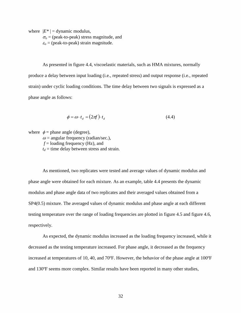
As presented in figure 4.4, viscoelastic materials, such as HMA mixtures, normally

produce a delay between input loading (i.e., repeated stress) and output response (i.e., repeated

strain) under cyclic loading conditions. The time delay between two signals is expressed as a

phase angle as follows:

dd tft 2 (4.4)

where = phase angle (degree),

= angular frequency (radian/sec.),

f = loading frequency (Hz), and

td = time delay between stress and strain.

As mentioned, two replicates were tested and average values of dynamic modulus and

phase angle were obtained for each mixture. As an example, table 4.4 presents the dynamic

modulus and phase angle data of two replicates and their averaged values obtained from a

SP4(0.5) mixture. The averaged values of dynamic modulus and phase angle at each different

testing temperature over the range of loading frequencies are plotted in figure 4.5 and figure 4.6,

respectively.

As expected, the dynamic modulus increased as the loading frequency increased, while it

decreased as the testing temperature increased. For phase angle, it decreased as the frequency

increased at temperatures of 10, 40, and 70ºF. However, the behavior of the phase angle at 100ºF

and 130ºF seems more complex. Similar results have been reported in many other studies,

33

including that by Flintsch et al. (2008). All 20 mixtures tested in this study showed similar

behavior.

Table 4.4 Dynamic Moduli and Phase Angles of SP4(0.5) NH281-4(119) Mixture

Temp.

(ºF)

Freq

(Hz)

#1 #2 Average

|E*| (psi) (º) |E*| (psi) (º) |E*| (psi) (º)

14

25 3706833.2 4.3 4158437.9 7.2 3932635.5 5.8

10 3649624.3 6.2 4029779.4 9.1 3839701.8 7.7

5 3276894.6 8.6 3768305.8 9.1 3522600.2 8.9

1 2927421.9 10.3 3319492.8 11.6 3123457.3 11.0

0.5 2774197.8 9.1 3140589.5 12.2 2957393.6 10.6

0.1 2681577.9 11.5 3024835.7 13.5 2853206.8 12.5

40

25 2705128.7 8.2 2469577.0 7.2 2587352.8 7.7

10 2596081.3 14.4 2279307.6 10.6 2437694.5 12.5

5 2366518.9 17.3 2067985.7 12.5 2217252.3 14.9

1 1779580.4 21.1 1628127.8 17.3 1703854.1 19.2

0.5 1537555.3 24.0 1439686.4 19.2 1488620.8 21.6

0.1 1326416.4 26.4 1246506.8 22.6 1286461.6 24.5

70

25 1081550.8 18.7 1103120.2 17.8 1092335.5 18.2

10 887793.4 23.4 914184.5 24.6 900989.0 24.0

5 702660.5 27.4 745089.1 23.3 723874.8 25.3

1 380178.6 33.1 410632.8 32.4 395405.7 32.8

0.5 271310.4 35.4 303462.3 32.8 287386.3 34.1

0.1 192383.6 32.7 216222.3 31.7 204302.9 32.2

100

25 283236.2 39.8 361721.7 27.4 322478.9 33.6

10 199252.3 30.8 269312.8 23.8 234282.6 27.3

5 148747.9 34.8 199533.1 28.9 174140.5 31.9

1 77095.0 35.0 97100.0 35.3 87097.5 35.2

0.5 64520.3 29.9 82343.5 32.2 73431.9 31.0

0.1 53189.2 27.4 64971.7 28.3 59080.4 27.8

130

25 83076.2 42.2 84895.4 36.0 83985.8 39.1

10 60024.0 29.8 65426.9 24.6 62725.5 27.2

5 50290.8 27.1 53320.8 27.0 51805.8 27.1

1 36749.1 27.0 39599.0 25.1 38174.1 26.1

0.5 33430.4 26.4 35626.5 26.8 34528.4 26.6

0.1 36346.9 25.2 37166.2 23.2 36756.5 24.2

34

1.0E+04

1.0E+05

1.0E+06

1.0E+07

0.01 0.10 1.00 10.00 100.00

Dyn

am

ic M

od

ulu

s (

ps

i)

Frequency (Hz)

14ºF 40ºF 70ºF 100ºF 130ºF

Figure 4.5 Plot of Averaged Dynamic Moduli: SP4(0.5) NH281-4(119) Mixture

0

10

20

30

40

50

0.01 0.10 1.00 10.00 100.00

Ph

as

e a

ng

le (

º)

Frequency (Hz)

14ºF 40ºF 70ºF 100ºF 130ºF

Figure 4.6 Plot of Averaged Phase Angles: SP4(0.5) NH281-4(119) Mixture

35

MEPDG requires the dynamic moduli for 30 temperature-frequency combinations (i.e.,

five temperatures and six frequencies) to conduct Level 1 design analysis. Therefore, the

dynamic modulus values of the 30 temperature-frequency combinations are presented in

Appendix A.

With the 30 individual dynamic moduli at all levels of temperature and frequency, the

MEPDG determined a stiffness master curve constructed at a reference temperature (generally

70°F). The master curve represents the stiffness of the material in a wide range of loading

frequencies (or loading times, equivalently). Master curves were constructed using the principle

of time (or frequency) - temperature superposition. The data at various temperatures were shifted

with respect to loading frequency until the curves merged into a single smooth function. The

master curve of the dynamic modulus as a function of time (or frequency), formed in this manner,

describes the time (or loading rate) dependency of the material. The amount of shifting at each

temperature required to form the master curve describes the temperature dependency of the

material. As an example, figure 4.7 shows a constructed master curve and its shift factors for a

mixture: SP4(0.5) NH281-4(119).

36

1.0E+04

1.0E+05

1.0E+06

1.0E+07

1.0E-08 1.0E-05 1.0E-02 1.0E+01 1.0E+04 1.0E+07

Dyn

am

ic M

od

ulu

s (

ps

i)

Reduced Frequency (Hz)

14 ºF

40 ºF

70 ºF

100 ºF

130 ºF

data shifted

sigmoidal fit

(a) Construction of a Master Curve

-4

-2

0

2

4

6

0 30 60 90 120 150

Lo

g S

hif

t fa

cto

r

Temperature (ºF)

(b) Shift Factors

Figure 4.7 Example of Developing a Master Curve and Its Shift Factors

37

As illustrated in figure 4.7(a), the modulus master curve can be mathematically modeled

by a sigmoidal function (Pellinen and Witczak 2002), described as follows:

rfeE

log

*

1log

(4.5)

where log|E* | = log of dynamic modulus,

= minimum modulus value,

fr = reduced frequency,

span of modulus values, and

shape parameters.

For Level 1 MEPDG analysis, the master curve and sigmoidal function parameters of

each mixture were determined using measured dynamic modulus test data as mentioned above.

Figures 4.8(a) through 4.8(e) present master curves of all 20 HMA mixtures: four HRB, four

SPL, four SP4(0.375), four SP4(0.5), and four SP5, respectively. Legends in each graph indicate

field project identifications as previously shown in table 3.1. From the figures, variations in

dynamic modulus values among mixtures can be observed even though they are the same type of

mixtures. This implies that mixture stiffness characteristics are related to properties and

proportioning of mixture constituents. Individual mixtures in the same mixture type were

produced by blending different mixture components.

Table 4.5 presents sigmoidal function parameters and shift factors for each mixture.

These model parameters and shift factors were utilized to develop master curves of each HMA

mixture. Using the values presented in the table, a new master curve at an arbitrary reference

temperature can be identified by simply moving the entire master curve in the horizontal

direction.

38

1.0E+04

1.0E+05

1.0E+06

1.0E+07

1.E-05 1.E-03 1.E-01 1.E+01 1.E+03 1.E+05 1.E+07

Reduced Frequncy (Hz)

Dy

na

mic

Mo

du

lus

(p

si)

RD 9-4(1012)

RD 81-2(1037)

STP 14-4(110)

NH 6-4(125)

(a) HRB Mixtures

1.0E+04

1.0E+05

1.0E+06

1.0E+07

1.E-05 1.E-03 1.E-01 1.E+01 1.E+03 1.E+05 1.E+07


Dy

na

mic

Mo

du

lus

(p

si)

STPD 6-6(156)

STPD 79-2(102)

STP 91-3(107)

NH-80-9(832),(825),(827)

(b) SPL Mixtures

Figure 4.8 Master Curves of Each Mixture at a Reference Temperature (70°F)

39

1.0E+04

1.0E+05

1.0E+06

1.0E+07

1.E-05 1.E-03 1.E-01 1.E+01 1.E+03 1.E+05 1.E+07


Dy

na

mic

Mo

du

lus

(p

si)

RD 81-2(1037)

RD 9-4(1012)

NH 6-4(125)

RD 25-2(1014)

(c) SP4(0.375) Mixtures

1.0E+04

1.0E+05

1.0E+06

1.0E+07

1.E-05 1.E-03 1.E-01 1.E+01 1.E+03 1.E+05 1.E+07


Dy

na

mic

Mo

du

lus

(p

si)

PEP 183-1(1020)

STPD-NFF

NH 281-4(119)

NH 83-3(107)

(d) SP4(0.5) Mixtures

Figure 4.8 Master Curves of Each Mixture at a Reference Temperature (70°F) cont’d

40

1.0E+04

1.0E+05

1.0E+06

1.0E+07

1.E-05 1.E-03 1.E-01 1.E+01 1.E+03 1.E+05 1.E+07


Dy

na

mic

Mo

du

lus

(p

si)

RD 75-2(1055)

STPD-6-7(178)

RD-77-2(1057)

IM 80-6(97)

(e) SP5 Mixtures

Figure 4.8 Master Curves of Each Mixture at a Reference Temperature (70°F) cont’d

41

Tab

le 4

.5 S

igm

oid

al F

unct

ion P

aram

eter

s an

d S

hif

t F

acto

rs o

f A

ll M

ixtu

res

Mix

Typ

e

Pro

ject

Nu

mb

er

δ

α

β

γ lo

g a

(14

) lo

g a

(40

) lo

g a

(70

) lo

g a

(10

0)

log a

(13

0)

A

VT

S

HR

B

RD

9-4

(1

01

2)

4.3

85

2

.12

0

-0.3

04

0.6

68

5.0

72

2.4

23

0

-1.9

37

-3.4

67

9.5

13

-3.1

55

RD

81

-2 (

10

37)

4.3

08

2

.06

5

-0.2

90

0.7

11

4.8

97

2.3

37

0

-1.8

64

-3.3

35

9.6

11

-3.1

90

ST

P 1

4-4

(1

10

) 4

.30

1

2.1

67

-0.1

26

0.6

73

4.9

09

2.3

44

0

-1.8

71

-3.3

47

9.5

87

-3.1

80

NH

6-4

(1

25

) 4

.27

7

2.2

03

0.2

32

0.7

45

4.7

23

2.2

91

0

-1.8

87

-3.4

20

8.0

59

-2.6

31

SP

L

ST

PD

6-6

(1

56

) 4

.39

3

2.1

11

-0.2

72

0.6

75

4.9

26

2.3

52

0

-1.8

78

-3.3

59

9.5

79

-3.1

77

ST

PD

79

-2 (

10

2)

4.1

58

2

.40

4

-0.6

04

0.5

48

5.5

81

2.6

55

0

-2.1

05

-3.7

56

9.9

10

-3.2

99

ST

P 9

1-3

(1

07

) 4

.39

6

2.0

04

-0.1

40

0.7

05

4.5

65

2.2

13

0

-1.8

21

-3.3

00

8.1

07

-2.6

46

NH

80

-9 (

83

2)

4.0

55

2

.47

5

-0.7

26

0.5

23

5.0

35

2.4

39

0

-2.0

01

-3.6

23

8.2

54

-2.6

88

SP

4

(0.3

75

)

RD

81

-2 (

10

37)

4.4

73

2

.05

4

-0.0

23

0.7

33

4.6

52

2.2

46

0

-1.8

32

-3.3

07

8.5

49

-2.7

99

RD

9-4

(1

01

2)

4.3

30

2

.11

1

0.0

20

0.6

91

4.5

60

2.1

97

0

-1.7

86

-3.2

20

8.7

08

-2.8

59

NH

6-4

(1

25

) 4

.32

2

2.2

33

-0.1

36

0.6

93

4.8

55

2.3

40

0

-1.9

02

-3.4

30

8.6

99

-2.8

56

RD

25

-2 (

10

14)

4.2

07

2

.30

2

-0.3

22

0.6

36

4.9

14

2.3

65

0

-1.9

17

-3.4

53

8.8

36

-2.9

06

SP

4

(0

.5)

PE

P 1

83

-1 (

102

0)

4.1

87

2

.30

7

-0.5

95

0.5

22

4.9

68

2.4

15

0

-1.9

96

-3.6

25

7.8

97

-2.5

60

ST

PD

-NF

F 1

1-2

(1

15)

6.4

73

-1

.90

7

0.0

94

-0.7

70

4.4

54

2.1

53

0

-1.7

60

-3.1

81

8.4

38

-2.7

57

NH

28

1-4

(1

19

) 4

.29

3

2.2

97

-0.3

29

0.6

15

4.9

04

2.3

62

0

-1.9

19

-3.4

58

8.7

41

-2.8

72

NH

83

-3 (

10

7)

6.5

67

-2

.43

2

0.2

91

-0.5

95

4.7

76

2.3

02

0

-1.8

71

-3.3

74

8.6

99

-2.8

56

SP

5

RD

75

-2 (

10

55)

4.3

19

2

.27

7

-0.7

95

0.5

28

4.9

99

2.4

23

0

-1.9

93

-3.6

10

8.1

61

-2.6

56

ST

PD

-6-7

(1

78

) 4

.11

5

2.4

53

-0.6

03

0.5

09

5.0

20

2.4

08

0

-1.9

40

-3.4

83

9.1

54

-3.0

19

RD

-77

-2 (

10

57)

4.2

79

2

.29

6

-0.4

06

0.5

39

4.8

35

2.3

26

0

-1.8

84

-3.3

92

8.8

74

-2.9

20

IM 8

0-6

(97

) 4

.30

9

2.2

61

-0.5

74

0.6

43

4.8

84

2.3

63

0

-1.9

36

-3.5

02

8.3

35

-2.7

21

42

4.1.3 Dynamic modulus characterization for Level 2 and Level 3 analysis

As mentioned in Chapter 2, one of the most interesting aspects of the MEPDG design

procedure is its hierarchical approach, i.e., the consideration of different levels of inputs. This

hierarchical approach enables the designer to select the design input level depending on the

degree of significance of the project and availability of resources. Each input level needs

different testing efforts and procedures to determine mixture dynamic modulus characteristics, as

presented in table 4.6.

Table 4.6 Dynamic Modulus Estimation at Various Hierarchical Input Levels

Input

Level Description

1

Conduct |E*| (dynamic modulus) laboratory test at loading frequencies and

temperatures of interest for the given mixture

Conduct binder complex shear modulus (G*) and phase angle () testing on the

proposed asphalt binder (AASHTO T315) at ω=1.59 Hz (10 rad/s) over a range

of temperatures

From binder test data estimate A-VTS for mix-compaction temperature

Develop master curve for the asphalt mixture that accurately defines the time-

temperature dependency including aging

2

No |E*| laboratory test required

Use |E*| predictive equation

Conduct binder complex shear modulus (G*) and phase angle () testing on the

proposed asphalt binder (AASHTO T315) at ω=1.59 Hz (10 rad/s) over a range

of temperatures. The binder viscosity or stiffness can also be estimated using

conventional asphalt test data such as Ring and Ball Softening Point, absolute

and kinematic viscosities, or using the Brookfield viscometer.

Develop A-VTS for mix-compaction temperature



3

No |E*| laboratory test required

Use |E*| predictive equation

Use typical A-VTS values provided in the Design Guide software based on PG,

viscosity, or penetration grade of the binder



As shown in the table, the Level 1 MEPDG design needs dynamic modulus tests at

different temperatures and loading frequencies, while Levels 2 and 3 do not require physical

43

modulus testing. Dynamic modulus master curves for Level 2 and 3 analyses were developed

using Witczak’s dynamic modulus predictive equation. This equation can predict the dynamic

modulus of asphalt mixtures over a range of temperatures, rates of loading, and aging conditions

by using information that is readily available from the volumetric mixture design.

The first version of Witczak’s predictive equation (Fonseca and Witczak 1996) was used

in the first development of the MEPDG interim guide (Andrei et al. 1999). In the interim guide,

MEPDG considered mixture volumetric properties and gradation, binder viscosity, and loading

frequency as input variables to predict the dynamic modulus of asphalt concrete mixtures.

Multivariate regression analysis of 2,750 experimental data was used to construct the 1999

version of the predictive |E*| expression. Later, the 1999 version of the predictive equation was

revised with more test data, which resulted in replacements of several model coefficients. The

predictive equation implemented in the current MEPDG version (NCHRP 1-37A 2004) is shown

in the following equation:

)log393532.0log31335.0603313.0(

34

2

38384

4

2

200200

*

1

005470.0)(000017.0003958.00021.0871977.3

802208.0058097.0002841.0

)(001767.002932.0750063.3log

f

abeff

beff

a

e

VV

VV

E

(4.6)

where |E*| = dynamic modulus of mixture (psi),

200 = % passing the No.200 sieve,

4 = cumulative % retained on the No.4 sieve,

38 = cumulative % retained on the 3/8 in. sieve,

34 = cumulative % retained on the 3/4 in. sieve,

Va = air void content (%),

Vbeff = effective binder content (% by volume),

f = loading frequency (Hz), and

= bitumen viscosity (106 Poise).

44

The viscosity of the asphalt binder at the temperature of interest is a critical input

parameter for the dynamic modulus characterization and the determination of shift factors, as

presented in table 4.6. For Level 1 and Level 2 design, the MEPDG required conducting binder

complex shear modulus (G*) and phase angle () testing on at ω=1.59 Hz (10 rad/s) over a range

of temperatures. The binder stiffness data obtained at different temperatures were then used to

calculate binder viscosity () and, correspondingly, two regression parameters (A and VTS),

which represent temperature susceptibility of the asphalt binder as previously described in

equations 4.1 and 4.2. On the other hand, Level 3 MEPDG analysis used typical A-VTS values

provided in the Design Guide software based on PG, viscosity, or penetration grade of the binder.

Figure 4.9 shows constructed master curves for Level 2 and 3 design analyses for all

HMA mixtures. For comparison, Level 1 master curves were also plotted in each graph. A

discrepancy between the Level 1 (measured) master curves and Level 2 or 3 (predicted) master

curves can be observed. The level of discrepancy between curves was mixture-specific, and was

generally larger at lower or higher loading frequencies. Differences between Level 2 and Level 3

master curves were not significant, since Witczak’s predictive model in equation 4.6 was used

for both cases.

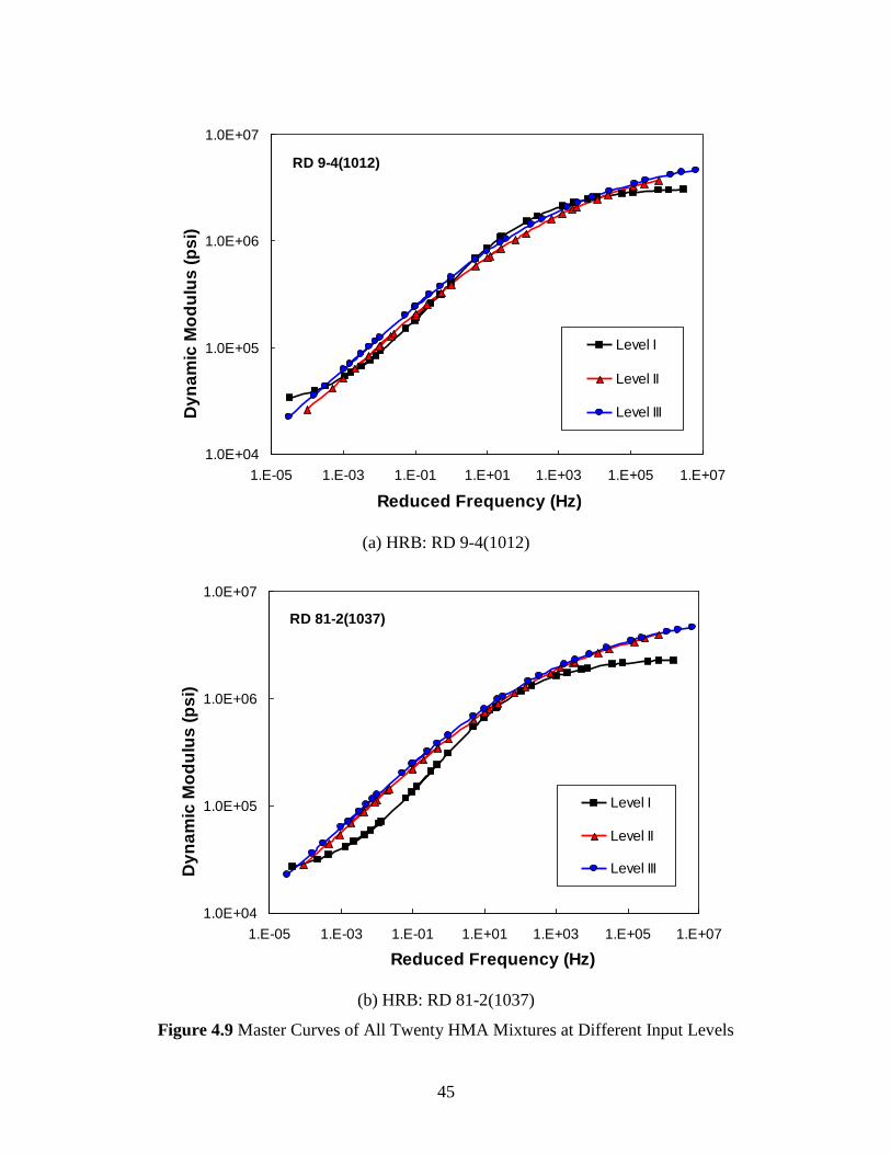
45

1.0E+04

1.0E+05

1.0E+06

1.0E+07

1.E-05 1.E-03 1.E-01 1.E+01 1.E+03 1.E+05 1.E+07


Dy

na

mic

Mo

du

lus

(p

si)

Level I

Level II

Level III

RD 9-4(1012)

(a) HRB: RD 9-4(1012)

1.0E+04

1.0E+05

1.0E+06

1.0E+07

1.E-05 1.E-03 1.E-01 1.E+01 1.E+03 1.E+05 1.E+07


Dy

na

mic

Mo

du

lus

(p

si)

Level I

Level II

Level III

RD 81-2(1037)

(b) HRB: RD 81-2(1037)

Figure 4.9 Master Curves of All Twenty HMA Mixtures at Different Input Levels

46

1.0E+04

1.0E+05

1.0E+06

1.0E+07

1.E-05 1.E-03 1.E-01 1.E+01 1.E+03 1.E+05 1.E+07


Dy

na

mic

Mo

du

lus

(p

si)

Level I

Level II

Level III

STP 14-4(110)

(c) HRB: STP 14-4(110)

1.0E+04

1.0E+05

1.0E+06

1.0E+07

1.E-05 1.E-03 1.E-01 1.E+01 1.E+03 1.E+05 1.E+07


Dy

na

mic

Mo

du

lus

(p

si)

Level I

Level II

Level III

NH 6-4(125)

(d) HRB: NH6-4(125)

Figure 4.9 Master Curves of All Twenty HMA Mixtures at Different Input Levels cont’d

47

1.0E+04

1.0E+05

1.0E+06

1.0E+07

1.E-05 1.E-03 1.E-01 1.E+01 1.E+03 1.E+05 1.E+07


Dy

na

mic

Mo

du

lus

(p

si)

Level I

Level II

Level III

STPD 6-6(156)

(e) SPL: STPD 6-6(156)

1.0E+04

1.0E+05

1.0E+06

1.0E+07

1.E-05 1.E-03 1.E-01 1.E+01 1.E+03 1.E+05 1.E+07


Dy

na

mic

Mo

du

lus

(p

si)

Level I

Level II

Level III

STPD 79-2(102)

(f) SPL: STPD 79-2(102)


48

1.0E+04

1.0E+05

1.0E+06

1.0E+07

1.E-05 1.E-03 1.E-01 1.E+01 1.E+03 1.E+05 1.E+07


Dy

na

mic

Mo

du

lus

(p

si)

Level I

Level II

Level III

STP 91-3(107)

(g) SPL: STP 91-3(107)

1.0E+04

1.0E+05

1.0E+06

1.0E+07

1.E-05 1.E-03 1.E-01 1.E+01 1.E+03 1.E+05 1.E+07


Dy

na

mic

Mo

du

lus

(p

si)

Level I

Level II

Level III

NH 80-9(832),(825),(827)

(h) SPL: NH 80-9 (832), (825), (827)


49

1.0E+04

1.0E+05

1.0E+06

1.0E+07

1.E-05 1.E-03 1.E-01 1.E+01 1.E+03 1.E+05 1.E+07


Dy

na

mic

Mo

du

lus

(p

si)

Level I

Level II

Level III

RD 81-2(1037)

(i) SP4(0.375): RD 81-2(1037)

1.0E+04

1.0E+05

1.0E+06

1.0E+07

1.E-05 1.E-03 1.E-01 1.E+01 1.E+03 1.E+05 1.E+07


Dy

na

mic

Mo

du

lus

(p

si)

Level I

Level II

Level III

RD 9-4(1012)

(j) SP4(0.375): RD 9-4(1012)


50

1.0E+04

1.0E+05

1.0E+06

1.0E+07

1.E-05 1.E-03 1.E-01 1.E+01 1.E+03 1.E+05 1.E+07


Dy

na

mic

Mo

du

lus

(p

si)

Level I

Level II

Level III

NH 6-4(125)

(k) SP4(0.375): NH 6-4(125)

1.0E+04

1.0E+05

1.0E+06

1.0E+07

1.E-05 1.E-03 1.E-01 1.E+01 1.E+03 1.E+05 1.E+07


Dy

na

mic

Mo

du

lus

(p

si)

Level I

Level II

Level III

RD 25-2(1014)

(l) SP4(0.375): RD 25-2(1014)


51

1.0E+04

1.0E+05

1.0E+06

1.0E+07

1.E-05 1.E-03 1.E-01 1.E+01 1.E+03 1.E+05 1.E+07


Dy

na

mic

Mo

du

lus

(p

si)

Level I

Level II

Level III

PEP 183-1(1020)

(m) SP4(0.5): PEP 183-1(1020)

1.0E+04

1.0E+05

1.0E+06

1.0E+07

1.E-05 1.E-03 1.E-01 1.E+01 1.E+03 1.E+05 1.E+07


Dy

na

mic

Mo

du

lus

(p

si)

Level I

Level II

Level III

STPD-NFF

(n) SP4(0.5): STPD-NFF 11-2(115)


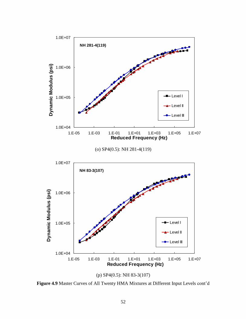
52

1.0E+04

1.0E+05

1.0E+06

1.0E+07

1.E-05 1.E-03 1.E-01 1.E+01 1.E+03 1.E+05 1.E+07


Dy

na

mic

Mo

du

lus

(p

si)

Level I

Level II

Level III

NH 281-4(119)

(o) SP4(0.5): NH 281-4(119)

1.0E+04

1.0E+05

1.0E+06

1.0E+07

1.E-05 1.E-03 1.E-01 1.E+01 1.E+03 1.E+05 1.E+07


Dy

na

mic

Mo

du

lus

(p

si)

Level I

Level II

Level III

NH 83-3(107)

(p) SP4(0.5): NH 83-3(107)


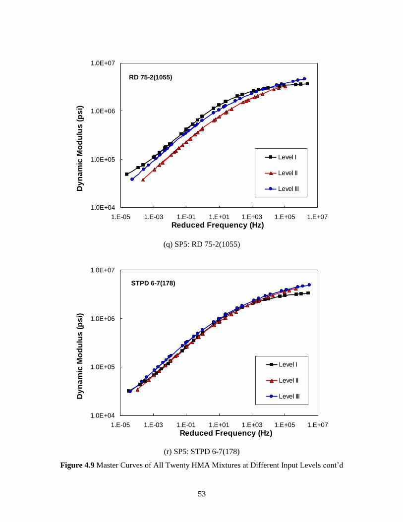
53

1.0E+04

1.0E+05

1.0E+06

1.0E+07

1.E-05 1.E-03 1.E-01 1.E+01 1.E+03 1.E+05 1.E+07


Dy

na

mic

Mo

du

lus

(p

si)

Level I

Level II

Level III

RD 75-2(1055)

(q) SP5: RD 75-2(1055)

1.0E+04

1.0E+05

1.0E+06

1.0E+07

1.E-05 1.E-03 1.E-01 1.E+01 1.E+03 1.E+05 1.E+07


Dy

na

mic

Mo

du

lus

(p

si)

Level I

Level II

Level III

STPD 6-7(178)

(r) SP5: STPD 6-7(178)


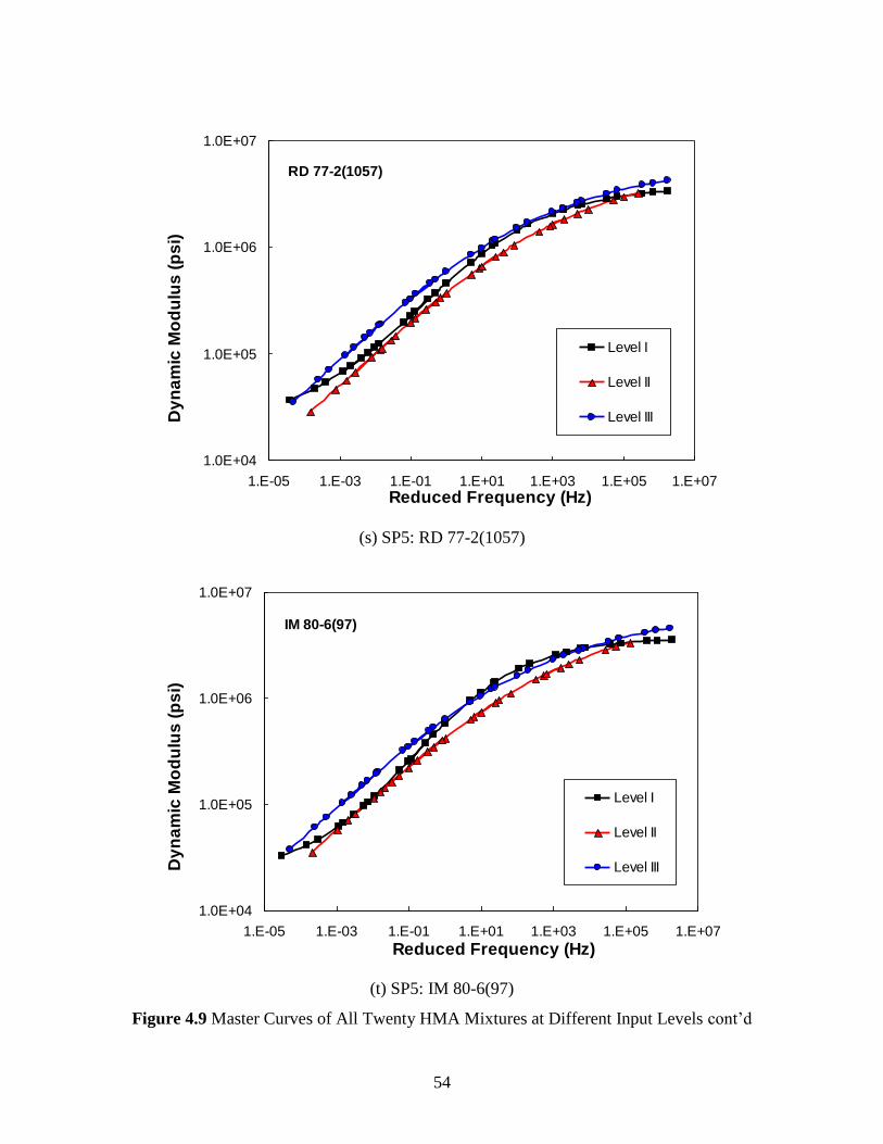
54

1.0E+04

1.0E+05

1.0E+06

1.0E+07

1.E-05 1.E-03 1.E-01 1.E+01 1.E+03 1.E+05 1.E+07


Dy

na

mic

Mo

du

lus

(p

si)

Level I

Level II

Level III

RD 77-2(1057)

(s) SP5: RD 77-2(1057)

1.0E+04

1.0E+05

1.0E+06

1.0E+07

1.E-05 1.E-03 1.E-01 1.E+01 1.E+03 1.E+05 1.E+07


Dy

na

mic

Mo

du

lus

(p

si)

Level I

Level II

Level III

IM 80-6(97)

(t) SP5: IM 80-6(97)


55

4.1.4 Creep compliance test (AASHTO T322)

The creep compliance test is used to describe the low-temperature behavior of asphalt

mixtures. It is the primary input for predicting thermal cracking in asphalt pavements over their

service lives. This test procedure is described in AASHTO T322. The current standard method

used in the United States to determine the creep compliance of asphalt mixtures is the indirect

tensile (IDT) test. In this study, the creep compliance test was conducted at 14°F.

A Superpave gyratory compactor was used to produce cylindrical samples with a

diameter of 150 mm and a height of 115 mm. The samples were then cut into specimens with a

diameter of 150 mm and a thickness of 38 mm. The target air void was 4% ± 0.5% for the testing

specimens. Figure 4.10 demonstrates the specimen production process using the Superpave

gyratory compactor, a saw machine, and the resulting specimen used to conduct the creep

compliance test.

Figure 4.10 Specimen Preparation Process for Creep Compliance Test

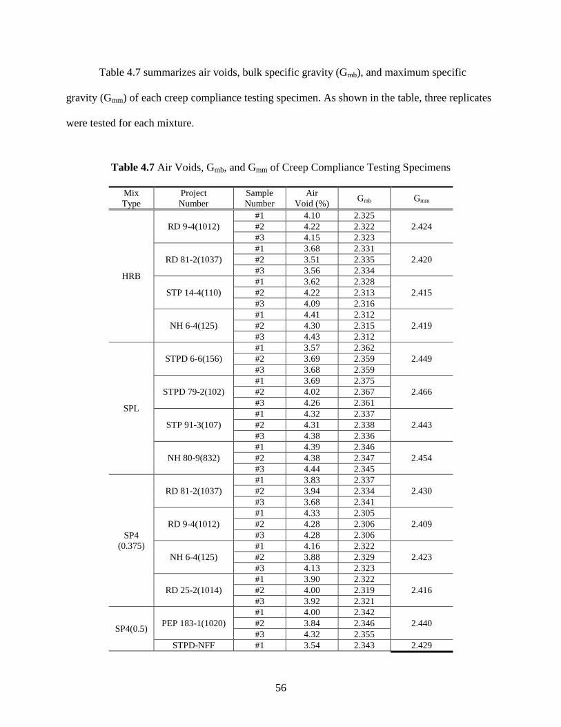
56

Table 4.7 summarizes air voids, bulk specific gravity (Gmb), and maximum specific

gravity (Gmm) of each creep compliance testing specimen. As shown in the table, three replicates

were tested for each mixture.

Table 4.7 Air Voids, Gmb, and Gmm of Creep Compliance Testing Specimens

Mix

Type

Project

Number

Sample

Number

Air

Void (%) Gmb Gmm

HRB

RD 9-4(1012)

#1 4.10 2.325

2.424 #2 4.22 2.322

#3 4.15 2.323

RD 81-2(1037)

#1 3.68 2.331

2.420 #2 3.51 2.335

#3 3.56 2.334

STP 14-4(110)

#1 3.62 2.328

2.415 #2 4.22 2.313

#3 4.09 2.316

NH 6-4(125)

#1 4.41 2.312

2.419 #2 4.30 2.315

#3 4.43 2.312

SPL

STPD 6-6(156)

#1 3.57 2.362

2.449 #2 3.69 2.359

#3 3.68 2.359

STPD 79-2(102)

#1 3.69 2.375

2.466 #2 4.02 2.367

#3 4.26 2.361

STP 91-3(107)

#1 4.32 2.337

2.443 #2 4.31 2.338

#3 4.38 2.336

NH 80-9(832)

#1 4.39 2.346

2.454 #2 4.38 2.347

#3 4.44 2.345

SP4

(0.375)

RD 81-2(1037)

#1 3.83 2.337

2.430 #2 3.94 2.334

#3 3.68 2.341

RD 9-4(1012)

#1 4.33 2.305

2.409 #2 4.28 2.306

#3 4.28 2.306

NH 6-4(125)

#1 4.16 2.322

2.423 #2 3.88 2.329

#3 4.13 2.323

RD 25-2(1014)

#1 3.90 2.322

2.416 #2 4.00 2.319

#3 3.92 2.321

SP4(0.5) PEP 183-1(1020)

#1 4.00 2.342

2.440 #2 3.84 2.346

#3 4.32 2.355

STPD-NFF #1 3.54 2.343 2.429

57

11-2 (115) #2 4.02 2.331

#3 4.22 2.326

NH 281-4(119)

#1 3.93 2.335

2.430 #2 3.96 2.334

#3 3.85 2.336

NH 83-3(107)

#1 4.24 2.324

2.427 #2 3.75 2.336

#3 4.34 2.322

SP5

RD 75-2(1055)

#1 3.58 2.360

2.448 #2 4.17 2.346

#3 4.37 2.341

STPD-6-7(178)

#1 3.77 2.349

2.441 #2 4.14 2.340

#3 4.13 2.340

RD-77-2(1057)

#1 3.93 2.367

2.464 #2 3.77 2.371

#3 3.96 2.366

IM 80-6(97)

#1 4.05 2.327

2.425 #2 4.29 2.321

#3 4.24 2.322

On each flat face of the specimen, two studs were placed along the vertical and two along

the horizontal axes, with a center-to-center spacing of 38 mm, so that two cross extensometers

could be mounted on the surfaces of the specimens (shown in fig. 4.11). The vertical and

horizontal displacements were recorded using the two cross extensometers during the test.

Figure 4.11 A Specimen with Extensometers Mounted in Testing Station

58

Once all three replicates of each mixture were tested, horizontal and vertical deformation

measurements of the six faces (three specimens and two faces per specimen) were recorded for

each specimen. The highest and lowest measurements of horizontal and vertical deformation

were then excluded so that the four middle measurements could be averaged. Finally, the creep

compliance of each mixture was determined by using the following equation, incorporating the

averaged measurements:

332.06354.0)(

1

Y

X

GLP

bdXtD (4.7)

where D(t) = creep compliance,

X = averaged horizontal deformation,

Y = averaged vertical deformation,

d = specimen diameter,

b = specimen thickness,

P = creep load, and

GL = gauge length.

In order to achieve the Level 1 MEPDG design, three temperatures (32°F, 14°F, and

−4°F) were used to determine the creep compliance of the mixtures, and a tensile strength test at

14°F was also performed. For the Level 2 MEPDG design, only one temperature (14°F) was

involved for the creep compliance and tensile strength testing of mixtures. On the other hand,

Level 3 analysis did not require physical testing at low temperatures. Creep compliance values at

three different temperatures (−4, 14, and 32°F) and the tensile strength at 14°F were

automatically generated by the MEPDG software, based on correlations with the mixtures’

volumetric characteristics and binder properties.

59

In this study, only the Level 2 creep compliance tests at 14°F were conducted. Level 1

creep compliance testing and the tensile strength test at 14°F could not be performed because of

the limited capability of the UTM-25kN testing equipment, which allows a loading level up to 25

kN and testing temperatures from 5°F to 140°F. The resulting Level 2 creep compliances at 14°F

of all 20 HMA mixtures are presented in figure 4.12. As can be observed from the figure, and

similar to the dynamic modulus test results, variations in creep compliance values among

mixtures exist even though the mixtures are of the same type. Since creep compliance values at

different loading times (i.e., 1, 2, 5, 10, 20, 50, and 100 seconds) were used as inputs for the

MEPDG simulations to predict the thermal cracking potential of pavements, the creep

compliance data at the seven discrete loading times were included in the database presented in

Appendix A. The tensile strength value at 14°F presented in the database was calculated using

the following regression equation, which has been implemented in the current MEPDG software:

AFPenVFA

VFAVVTS aa

log296.203977log71.405704.0

592.122304.0016.114712.7416

2

2

(4.8)

where TS = indirect tensile strength (psi) at 14 ºF,

Va = air void content (%),

VFA = voids filled with asphalt (%),

Pen77F = binder penetration at 77 ºF (dmm), and

A = viscosity – temperature susceptibility intercept.

60

1.0E-08

1.0E-06

1.0E-04

1 10 100

Time (sec)

Cre

ep

Co

mp

lia

nc

e (

1/p

si)

RD 9-4(1012)

RD 81-2(1037)

STP 14-4(110)

NH 6-4(125)

(a) HRB Mixtures

1.0E-08

1.0E-06

1.0E-04

1 10 100

Time (sec)

Cre

ep

Co

mp

lia

nc

e (

1/p

si)

STPD 6-6(156)

STPD 79-2(102)

STP 91-3(107)

NH 80-9(832),(825),(827)

(b) SPL Mixtures

Figure 4.12 Creep Compliance at 14°F of All HMA Mixtures

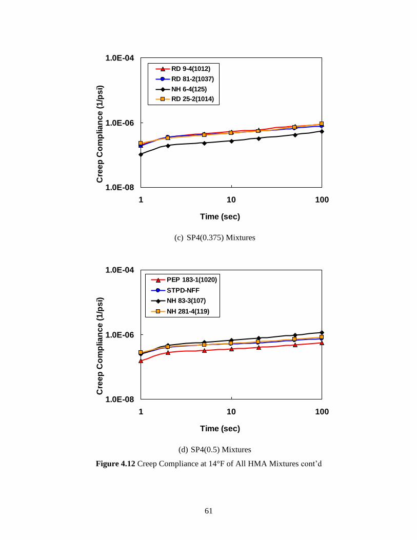
61

1.0E-08

1.0E-06

1.0E-04

1 10 100

Time (sec)

Cre

ep

Co

mp

lia

nc

e (

1/p

si)

RD 9-4(1012)

RD 81-2(1037)

NH 6-4(125)

RD 25-2(1014)

(c) SP4(0.375) Mixtures

1.0E-08

1.0E-06

1.0E-04

1 10 100

Time (sec)

Cre

ep

Co

mp

lia

nc

e (

1/p

si)

PEP 183-1(1020)

STPD-NFF

NH 83-3(107)

NH 281-4(119)

(d) SP4(0.5) Mixtures

Figure 4.12 Creep Compliance at 14°F of All HMA Mixtures cont’d

62

1.0E-08

1.0E-06

1.0E-04

1 10 100

Time (sec)

Cre

ep

Co

mp

lia

nc

e (

1/p

si)

RD 75-2(1055)

RD 77-2(1057)

STPD 6-7(178)

IM 80-6(97)

(e) SP5 Mixtures

Figure 4.12 Creep Compliance at 14°F of All HMA Mixtures cont’d

As previously mentioned, the Level 3 analysis can also be conducted using creep

compliance and tensile strength data produced by MEPDG software, based on correlations with

mixture volumetric characteristics and binder properties. Similar to the regression equation for

the tensile strength of the mixture, time-varying creep compliance data are obtained by the

following equations:

63

mtDtD 1)( (4.9)

AVFAVTD a log923.1log0103.2log7957.001306.0524.8log 1 (4.10)

4605.077001638.0

7700247.001126.004596.000185.01628.1

FPenT

FPenVFAVTm a

(4.11)

where D(t) = creep compliance (1/psi),

D1 and m = creep compliance model parameters, and

T = testing temperature (F).

Figure 4.13 compares creep compliance results obtained from the Level 2 testing to the

calculated creep compliance values using equation 4.11 for Level 3 analysis. A mixture-specific

discrepancy can be observed between Level 2 (measured) curves and Level 3 (calculated) curves.

Differences between Level 2 and Level 3, shown in the figure, would affect low temperature

cracking performance of pavements.

64

1.0E-08

1.0E-06

1.0E-04

1 10 100

Time (sec)

Cre

ep

Co

mp

lia

nc

e (

1/p

si)

Level 2 Level 3

RD 9-4(1012)

(a) HRB: RD 9-4(1012)

1.0E-08

1.0E-06

1.0E-04

1 10 100

Time (sec)

Cre

ep

Co

mp

lia

nc

e (

1/p

si)

Level 2 Level 3

RD 81-2(1037)

(b) HRB: RD 81-2(1037)

Figure 4.13 Creep Compliance Results: Level 2 vs. Level 3

65

1.0E-08

1.0E-06

1.0E-04

1 10 100

Time (sec)

Cre

ep

Co

mp

lia

nc

e (

1/p

si)

Level 2 Level 3

STP 14-4(110)

(c) HRB: STP 14-4(110)

1.0E-08

1.0E-06

1.0E-04

1 10 100

Time (sec)

Cre

ep

Co

mp

lia

nc

e (

1/p

si)

Level 2 Level 3

NH 6-4(125)

(d) HRB: NH6-4(125)

Figure 4.13 Creep Compliance Results: Level 2 vs. Level 3 cont’d

66

1.0E-08

1.0E-06

1.0E-04

1 10 100

Time (sec)

Cre

ep

Co

mp

lia

nc

e (

1/p

si)

Level 2 Level 3

STPD 6-6(156)

(e) SPL: STPD 6-6(156)

1.0E-08

1.0E-06

1.0E-04

1 10 100

Time (sec)

Cre

ep

Co

mp

lia

nc

e (

1/p

si)

Level 2 Level 3

STPD 79-2(102)

(f) SPL: STPD 79-2(102)


67

1.0E-08

1.0E-06

1.0E-04

1 10 100

Time (sec)

Cre

ep

Co

mp

lia

nc

e (

1/p

si)

Level 2 Level 3

STP 91-3(107)

(g) SPL: STP 91-3(107)

1.0E-08

1.0E-06

1.0E-04

1 10 100

Time (sec)

Cre

ep

Co

mp

lia

nc

e (

1/p

si)

Level 2 Level 3

NH 80-9(832),(825), (827)

(h) SPL: NH 80-9 (832), (825), (827)


68

1.0E-08

1.0E-06

1.0E-04

1 10 100

Time (sec)

Cre

ep

Co

mp

lia

nc

e (

1/p

si)

Level 2 Level 3

RD 81-2(1037)

(i) SP4(0.375): RD 81-2(1037)

1.0E-08

1.0E-06

1.0E-04

1 10 100

Time (sec)

Cre

ep

Co

mp

lia

nc

e (

1/p

si)

Level 2 Level 3

RD 9-4(1012)

(j) SP4(0.375): RD 9-4(1012)


69

1.0E-08

1.0E-06

1.0E-04

1 10 100

Time (sec)

Cre

ep

Co

mp

lia

nc

e (

1/p

si)

Level 2 Level 3

NH 6-4(125)

(k) SP4(0.375): NH 6-4(125)

1.0E-08

1.0E-06

1.0E-04

1 10 100

Time (sec)

Cre

ep

Co

mp

lia

nc

e (

1/p

si)

Level 2 Level 3

RD 25-2(1014)

(l) SP4(0.375): RD 25-2(1014)


70

1.0E-08

1.0E-06

1.0E-04

1 10 100

Time (sec)

Cre

ep

Co

mp

lia

nc

e (

1/p

si)

Level 2 Level 3

PEP 183-1(1020)

(m) SP4(0.5): PEP 183-1(1020)

1.0E-08

1.0E-06

1.0E-04

1 10 100

Time (sec)

Cre

ep

Co

mp

lia

nc

e (

1/p

si)

Level 2 Level 3

STPD-NFF

(n) SP4(0.5): STPD-NFF 11-2(115)


71

1.0E-08

1.0E-06

1.0E-04

1 10 100

Time (sec)

Cre

ep

Co

mp

lia

nc

e (

1/p

si)

Level 2 Level 3

NH 281-4(119)

(o) SP4(0.5): NH 281-4(119)

1.0E-08

1.0E-06

1.0E-04

1 10 100

Time (sec)

Cre

ep

Co

mp

lia

nc

e (

1/p

si)

Level 2 Level 3

NH 83-3(107)

(p) SP4(0.5): NH 83-3(107)


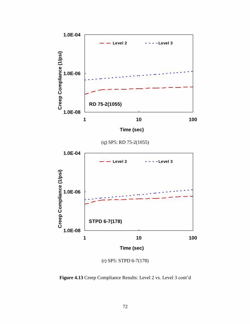
72

1.0E-08

1.0E-06

1.0E-04

1 10 100

Time (sec)

Cre

ep

Co

mp

lia

nc

e (

1/p

si)

Level 2 Level 3

RD 75-2(1055)

(q) SP5: RD 75-2(1055)

1.0E-08

1.0E-06

1.0E-04

1 10 100

Time (sec)

Cre

ep

Co

mp

lia

nc

e (

1/p

si)

Level 2 Level 3

STPD 6-7(178)

(r) SP5: STPD 6-7(178)


73

1.0E-08

1.0E-06

1.0E-04

1 10 100

Time (sec)

Cre

ep

Co

mp

lia

nc

e (

1/p

si)

Level 2 Level 3

RD 77-2(1057)

(s) SP5: RD 77-2(1057)

1.0E-08

1.0E-06

1.0E-04

1 10 100

Time (sec)

Cre

ep

Co

mp

lia

nc

e (

1/p

si)

Level 2 Level 3

IM 80-6(97)

(t) SP5: IM 80-6(97)


74

4.2 Tests and Results of Subgrade Soils

Layer stiffness characteristics of subgrade soils in the MEPDG analysis are represented

by resilient modulus. As mentioned earlier, the triaxial resilient modulus test is conducted for

Level 1 analysis, whereas basic physical properties of soils, such as specific gravity, Atterberg

limits, and particle size gradations, are used as necessary information to conduct Level 2 or 3

analysis.

Three native unbound soils (loess, loess/till, and sandy silt) were selected for this

research as representative subgrade soils often used in Nebraska pavements. They were tested to

evaluate all aforementioned physical properties and resilient modulus characteristics so that all

three levels of MEPDG analysis could be performed. In addition to the three unbound soils, nine

stabilized soils (loess, till, and shale stabilized with hydrated lime, fly ash and cement kiln dust,

respectively), which were studied by Hensley et al. (2007) for a previous NDOR research project,

were also included in this study to characterize their resilient modulus properties. Hensley et al.

(2007) tested the nine stabilized soils compacted with an optimum amount of different types of

pozzolans. The three unbound soils and the nine stabilized soils are expected to provide a more

general and comprehensive resilient modulus database of the types of subgrade soils that are

often applied to various Nebraska pavement projects.

4.2.1 Physical properties of unbound soils

Table 4.8 summarizes the physical property tests considered, their standard methods used,

and test results for the three unbound soils: loess, loess/till, and sandy silt. All tests were

performed at the UNL soils laboratory, and representative soil samples were then sent to the

NDOR geotechnical laboratory for validation. As can be seen in the table, physical properties

obtained from the UNL laboratory were very close to NDOR measurements.

75

Table 4.8 Summary of Physical Property Tests and Results of Three Unbound Soils

Physical Property Standard

Method

Sandy Silt Loess Loess/Till

UNL NDOR UNL NDOR UNL NDOR

Specific Gravity AASHTO T100 2.61 N/A 2.65 N/A 2.71 N/A

Liquid Limit AASHTO T89 28 29 25 25 40 41

Plastic Limit AASHTO T90 20 21 22 23 19 20

Plasticity Index AASHTO T90 8 8 3 2 21 21

Ret. % Sieve No.200 AASHTO T88 37 40 9 10 0.5 1

Group Classification AASHTO M145 A-4 A-4 A-4 A-4 A-6 A-6

4.2.2 Standard proctor test results of unbound soils

The optimum moisture content and the maximum dry unit weight were determined by

performing compaction tests on each soil, based on the standard testing method, AASHTO T99:

Moisture-Density Relations of Soils Using a 5.5 lb Rammer and a 12 in. Drop. Soils were

compacted using a mechanical compactor to produce cylindrical specimens of 4 in. (100 mm) in

diameter and 4 in. (100 mm) high. The test results were then plotted on a dry unit weight vs.

moisture content diagram, as shown in figure 4.14.

76

80

85

90

95

100

105

110

0 5 10 15 20 25 30 35

Moisture Content (%)

Dry

Un

it W

eig

ht

(lb

/ft^

3)

Loess

Loess/Till

Sandy Silt

Figure 4.14 Plots of Compaction Curves

The curve connecting the data points represents the dry unit weight achieved by

compacting the soil at various moisture contents. Higher dry unit weight values indicate higher

quality fill, so there is a certain moisture content, known as the optimum moisture content, that

produces the greatest dry unit weight. The greatest dry unit weight is called the maximum dry

unit weight. Table 4.9 presents the optimum moisture content and the corresponding maximum

dry unit weight of the three unbound soils, determined from figure 4.14.

77

Table 4.9 Summary of Standard Proctor Test Results

Unbound Soil Loess Loess/Till Sandy Silt

Optimum Moisture

Content (%) 16.5 20.3 13.0

Maximum Dry

Unit Weight (lb/ft3)

106 104 108

4.2.3 Resilient modulus test of unbound soils

The resilient modulus represents the elastic response of a material under simulated,

repeated traffic loading. Most paving materials are not elastic, but instead they deform plastically

after each load application. However, if the load is small compared to the strength of the material

and is repeated numerous times, the deformation under each load application is almost

completely recoverable and proportional to the load, so it can be considered elastic (Huang 1993).

The response of a soil specimen under repeated loads is illustrated in figure 4.15. As shown in

the figure, the total strain is composed of plastic strain, which is called permanent strain, and

elastic strain. Considerable plastic strain occurs during the initial loading stage, but as the

number of repetitions increases, the increasing rate of plastic strain decreases. After 150 to 200

load repetitions, the cumulative plastic strain approaches a constant level. The resilient modulus

is defined as elastic modulus based on recoverable (resilient) strain under repeated loads,

expressed by:

78

r

dRM

(4.12)

where MR = resilient modulus,

d = deviator stress, and

r = recoverable (resilient) strain.

Figure 4.15 General Response of a Soil Specimen under Repeated Load

The deviator stress is the axial stress in an unconfined compression test or the axial stress

in excess of the confining pressure in a triaxial compression test. Figure 4.16 shows confining

pressure (c) and deviator stress (d) for a cylindrical specimen in a triaxial test.

Total Strain

Resilient

Strain

Plastic Strain

Time

Strain

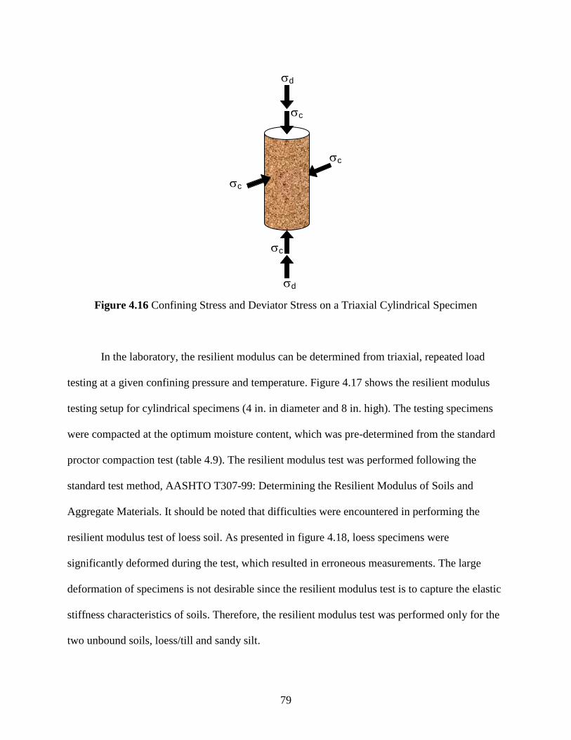
79

Figure 4.16 Confining Stress and Deviator Stress on a Triaxial Cylindrical Specimen

In the laboratory, the resilient modulus can be determined from triaxial, repeated load

testing at a given confining pressure and temperature. Figure 4.17 shows the resilient modulus

testing setup for cylindrical specimens (4 in. in diameter and 8 in. high). The testing specimens

were compacted at the optimum moisture content, which was pre-determined from the standard

proctor compaction test (table 4.9). The resilient modulus test was performed following the

standard test method, AASHTO T307-99: Determining the Resilient Modulus of Soils and

Aggregate Materials. It should be noted that difficulties were encountered in performing the

resilient modulus test of loess soil. As presented in figure 4.18, loess specimens were

significantly deformed during the test, which resulted in erroneous measurements. The large

deformation of specimens is not desirable since the resilient modulus test is to capture the elastic

stiffness characteristics of soils. Therefore, the resilient modulus test was performed only for the

two unbound soils, loess/till and sandy silt.

d

d

c

c

c

c

80

Figure 4.17 Resilient Modulus Testing Setup (AASHTO T307)

Figure 4.18 Specimens before and after Resilient Modulus Testing

Following the standard method, AASHTO T307-99, each soil specimen was prepared by

hand-mixing at the optimum moisture content. The moistened soil was then cured for 24 hours in

a sealed plastic bag before it was compacted to produce cylindrical specimens. After compaction,

a latex membrane was sealed onto the specimen surface to apply the pre-conditioning process

and the designated series of confining pressure and deviator stress. For each specimen, the

resilient modulus was determined for 15 consecutive stress states at confining pressure, ranging

Before After Before After

LOESS LOESS/TILL

81

from 2 to 6 psi and deviator stress between 2 and 10 psi. Table 4.10 presents the 15 combinations

of confining pressure and deviator stress specified in the testing protocol: AASHTO T307.

Table 4.10 Combinations of Confining Pressure and Deviator Stress Applied

Sequence

No.

Confining

Pressure (psi)

Deviator

Stress (psi)

Cyclic Stress

(psi)

Constant

Stress (psi)

No. of Load

Applications

1 6.0 2 1.8 0.2 100

2 6.0 4 3.6 0.4 100

3 6.0 6 5.4 0.6 100

4 6.0 8 7.2 0.8 100

5 6.0 10 9.0 1.0 100

6 4.0 2 1.8 0.2 100

7 4.0 4 3.6 0.4 100

8 4.0 6 5.4 0.6 100

9 4.0 8 7.2 0.8 100

10 4.0 10 9.0 1.0 100

11 2.0 2 1.8 0.2 100

12 2.0 4 3.6 0.4 100

13 2.0 6 5.4 0.6 100

14 2.0 8 7.2 0.8 100

15 2.0 10 9.0 1.0 100

4.2.4 Resilient modulus test results of unbound soils

Figure 4.19 shows representative resilient modulus test results from specimen No. 1 of

loess/till soil. The figure clearly demonstrates that the resilient modulus of the soil is a function

of both the confining pressure and the deviator stress, which implies that the soil stiffness is

stress-state dependent.

82

100

1000

10000

0 2 4 6 8 10

Deviator Stress (psi)

Resil

ien

t M

od

ulu

s (

psi)

Confining pressure = 6 psi



Figure 4.19 Resilient Modulus Test Results of Loess/Till Soil Specimen

Stress states (i.e., confining pressure and deviator stress) used for the resilient modulus

test were based on the depth at which the soils were located within the pavement structure and

the traffic loads applied to the pavement structure. In the MEPDG, the stress-dependent resilient

modulus of soils was characterized using a generalized constitutive model. The nonlinear elastic

coefficients and exponents of the generalized constitutive model were determined through

nonlinear regression analyses by fitting the model to laboratory resilient modulus test results.

The generalized constitutive model used in the MEPDG design procedure is as follows:

32

11

k

a

oct

k

a

aRPP

PkM

(4.13)

where MR = resilient modulus,

= 1st stress invariant = 3c + d,

c and d = confining stress and deviator stress, respectively,

Pa = atmospheric pressure (101.3 kPa or 14.7 psi),

oct = octahedral shear stress which is equal to d32 , and

k1, k2, k3 = model parameters.

83

The constitutive model parameters (k1, k2, k3) for each test material should be determined

with a high level of correlation to test data. Generally, R2-value (called a coefficient of

determination) exceeding 0.90 is recommended. To obtain model parameters of each soil in a

more general sense, resilient modulus test results of multiple specimens (i.e., three for loess/till

and four for sandy silt) were used together. Figure 4.20 presents cross-plots between measured

moduli and predicted moduli using the model (equation 4.13) after finding the three model

parameters. As indicated by the coefficient of determination (R2) values, the model fits test

results very well, which implies that the model can be appropriately used to represent stress-

dependent behavior of each soil in a pavement structure.

Table 4.11 presents resulting model parameters. The parameter k2 is positive, indicating

that an increase in confinement causes an increase in the modulus, while the parameter k3 is

negative, indicating that an increase in the deviator stress causes a reduction in the resilient

modulus. The work by Uzan (1985) has shown that a decrease in resilient modulus, with an

increase in deviator stress, occurs when the ratio of the major principal stress to minor principal

stress is lower than 2 or 3, depending on the soil type. Notably, the input data required for the

Level 1 MEPDG analysis are not the actual resilient modulus test data but the three model

parameters. Therefore, the nonlinear regression process to identify the model parameters needs to

be conducted to operate the Level 1 analysis.

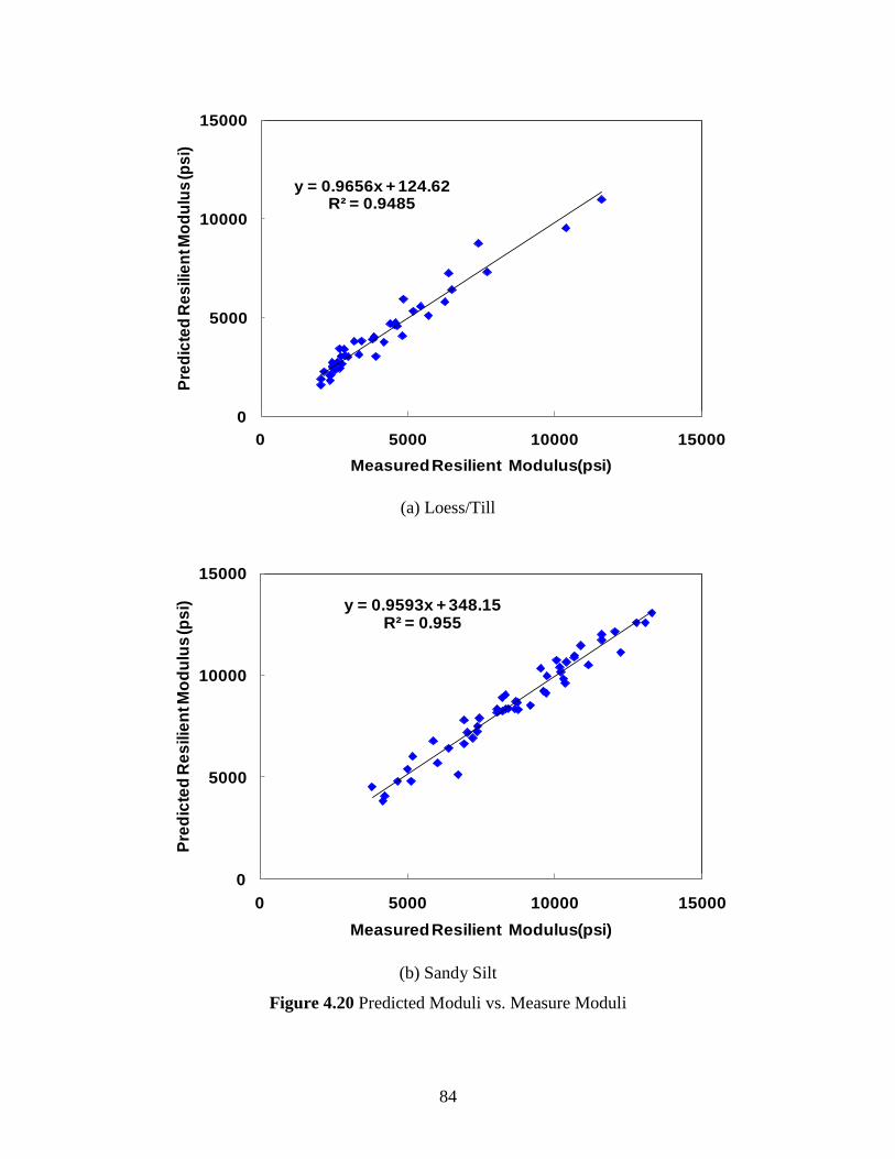
84

y = 0.9656x + 124.62R² = 0.9485

0

5000

10000

15000

0 5000 10000 15000

Pre

dic

ted

Re

silie

nt M

od

ulu

s (p

si)

Measured Resilient Modulus(psi)

(a) Loess/Till

y = 0.9593x + 348.15R² = 0.955

0

5000

10000

15000

0 5000 10000 15000

Pre

dic

ted

Re

silie

nt M

od

ulu

s (p

si)

Measured Resilient Modulus(psi)

(b) Sandy Silt

Figure 4.20 Predicted Moduli vs. Measure Moduli

85

Table 4.11 Resulting Model Parameters and R2-value of Each Soil

k1 k2 k3 R2

Loess/Till 723.3492 0.580731 -6.79546 0.949

Sandy Silt 772.2054 0.474492 -2.12098 0.955

In addition to the two native unbound soils (i.e., loess/till and sandy silt) tested for the

Level 1 resilient modulus characterization, as previously mentioned, the resilient modulus

characteristics were also determined for the nine stabilized soils (loess, till, and shale stabilized

with hydrated lime [HL], fly ash [FA], and cement kiln dust [CKD], respectively). These soils

were studied by Hensley et al. (2007) for a previous NDOR research project. Raw test data

presented in Hensley et al. (2007) were used, and the resulting Level 1 model parameters are

summarized in table 4.12. The database presented in tables 4.11 and 4.12 and in Appendix B is

expected to provide a general input set of subgrade soils that are often used in Nebraska

pavement projects.

Table 4.12 Level 1 Resilient Modulus Model Parameters of Nine Stabilized Soils

Loess Till Shale

7%

CKD

12%

FA

5%

HL

7%

CKD

12%

FA

5%

HL

7%

CKD

14%

FA

6%

HL

k1 1985.2 802.4 1109.3 2564.5 1864.2 2061.8 2007.3 1063.5 1823.0

k2 0.367 0.392 0.414 0.467 0.420 0.311 0.395 0.455 0.364

k3 -1.081 -2.597 -2.601 -0.975 -0.917 -0.843 -0.744 -2.431 -1.219

R2 0.971 0.995 0.951 0.857 0.936 0.969 0.970 0.930 0.970

86

4.2.5 Resilient modulus values for Level 2 MEPDG analysis

When the Level 1 resilient modulus laboratory test (AASHTO T307) is not performed,

the user is then able to consider Level 2 analysis using the relationships between resilient

modulus and other soil properties, such as the California bearing ratio (CBR) or R-value. Table

4.13 shows these types of correlations with other soil characteristics. Accordingly, the Level 2

resilient modulus is not stress-dependent, but instead is a constant value. Table 4.14 presents a

single resilient modulus value for each soil considered in this research for the Level 2 MEPDG

analysis.

Table 4.13 Models Relating Material Properties to MR (NCHRP 1-37A 2004)

Model Comments Test Standard

CBR MR (psi) = 2555(CBR)0.64

(TPL) CBR = California Bearing Ratio AASHTO T193

R-value MR (psi) = 1155+555R(20) R = R value AASHTO T190

AASHTO

layer

coefficient MR (psi) = 30000(ai/0.14)(20) ai = AASHTO layer coefficient

AASHTO Guide

for the Design of

Pavement

PI and

Gradation CBR (%) = 75/{1+0.728(wPI)}

wPI = P200*PI

P200 = % passing No. 200 sieve,

PI = plasticity index (%)

AASHTO T27,

AASHTO T90

DCP CBR (%) = 292/DCP1.12

CBR= California Bearing Ratio,

DCP = DCP index (mm/blow) ASTM D6951

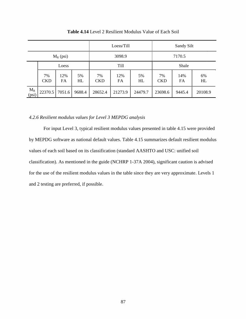
87

Table 4.14 Level 2 Resilient Modulus Value of Each Soil

Loess/Till Sandy Silt

MR (psi) 3098.9 7170.5

Loess Till Shale

7%

CKD

12%

FA

5%

HL

7%

CKD

12%

FA

5%

HL

7%

CKD

14%

FA

6%

HL

MR

(psi) 22370.5 7051.6 9688.4 28652.4 21273.9 24479.7 23698.6 9445.4 20108.9

4.2.6 Resilient modulus values for Level 3 MEPDG analysis

For input Level 3, typical resilient modulus values presented in table 4.15 were provided

by MEPDG software as national default values. Table 4.15 summarizes default resilient modulus

values of each soil based on its classification (standard AASHTO and USC: unified soil

classification). As mentioned in the guide (NCHRP 1-37A 2004), significant caution is advised

for the use of the resilient modulus values in the table since they are very approximate. Levels 1

and 2 testing are preferred, if possible.

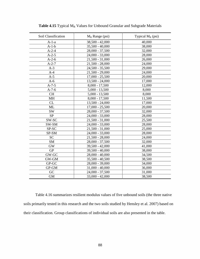
88

Table 4.15 Typical MR Values for Unbound Granular and Subgrade Materials

Soil Classification MR Range (psi) Typical MR (psi)

A-1-a 38,500 - 42,000 40,000

A-1-b 35,500 - 40,000 38,000

A-2-4 28,000 - 37,500 32,000

A-2-5 24,000 - 33,000 28,000

A-2-6 21,500 - 31,000 26,000

A-2-7 21,500 - 28,000 24,000

A-3 24,500 - 35,500 29,000

A-4 21,500 - 29,000 24,000

A-5 17,000 - 25,500 20,000

A-6 13,500 - 24,000 17,000

A-7-5 8,000 - 17,500 12,000

A-7-6 5,000 - 13,500 8,000

CH 5,000 - 13,500 8,000

MH 8,000 - 17,500 11,500

CL 13,500 - 24,000 17,000

ML 17,000 - 25,500 20,000

SW 28,000 - 37,500 32,000

SP 24,000 - 33,000 28,000

SW-SC 21,500 - 31,000 25,500

SW-SM 24,000 - 33,000 28,000

SP-SC 21,500 - 31,000 25,000

SP-SM 24,000 - 33,000 28,000

SC 21,500 - 28,000 24,000

SM 28,000 - 37,500 32,000

GW 39,500 - 42,000 41,000

GP 39,500 - 40,000 38,000

GW-GC 28,000 - 40,000 34,500

GW-GM 35,500 - 40,500 38,500

GP-GC 28,000 - 39,000 34,000

GP-GM 31,000 - 40,000 36,000

GC 24,000 - 37,500 31,000

GM 33,000 - 42,000 38,500

Table 4.16 summarizes resilient modulus values of five unbound soils (the three native

soils primarily tested in this research and the two soils studied by Hensley et al. 2007) based on

their classification. Group classifications of individual soils are also presented in the table.

89

Table 4.16 Level 3 Resilient Modulus Values Based on Group Classification

Type of Soil Sandy Silt Loess Loess/Till Till Shale

Group Classification A-4 A-4 A-6 A-6 A-7-5

MR (psi) 16,500 16,500 14,500 14,500 13,000

90

Chapter 5 MEPDG Sensitivity Analysis

For this chapter, MEPDG sensitivity analyses were conducted to evaluate the effects of

using different design level inputs on MEPDG performance predictions of asphalt pavement

structures. Each design level input of asphalt and soil materials presented in the previous chapter

was used for the MEPDG analyses, and resulting performance data between levels were

compared to examine sensitivity of MEPDG performance prediction depending on input levels.

To this end, the sensitivity analysis was conducted for typical full-depth flexible pavement

structures that have usually been implemented in Nebraska. Different levels of layer properties

and material characteristics presented in the database were incorporated with the typical full-

depth pavement structures to examine MEPDG performance sensitivities relating to the input

level of layer moduli. The most recent version (1.10) of MEPDG software was used for

simulations.

5.1 Sensitivity Analysis of Typical Pavement Structures

Nebraska flexible pavements are generally full-depth pavements with a design based on

the 1993 AASHTO Pavement Design Guide. When a new flexible pavement is designed, the

volume of heavy trucks (vehicle Class 4 to 13 shown in fig. 5.1) expected on the specific project

site is the primary factor considered for determining the pavement structure geometry with its

type of HMA mixture. In cases where fewer than 200 heavy trucks per day are expected, a

minimum HMA layer thickness of 8 in. is usually applied. If more than 200 heavy trucks per day

are expected, the minimum HMA layer thickness is 10 in., while a minimum HMA layer

thickness of 12 in. is necessary for the cases with more than 1,500 heavy trucks per day.

91

Figure 5.1 FHWA Vehicle Classification

The type of HMA mixture is also based on the volume of heavy trucks. In general, SPR

mixtures have been used as base asphalt mixtures or surface layer mixtures for Nebraska

highways subject to fewer than 200 trucks per day. SP4 Special mixtures are typically used for

surface layers for low-volume highways with 200-500 trucks per day, and SP4 mixtures are

applied to asphalt surface layers of pavements where 500-1,500 trucks are expected per day. SP5

mixtures are typically used for high volume highways with more than 1,500 heavy trucks

traveling daily. Finally, SPL and HRB mixtures are usually used as base layer materials. An

approximately 8 in. thick subgrade layer is then placed under the asphalt layers. The subgrade

materials are usually stabilized with fly ash or hydrated lime.

Figure 5.2 presents three typical full-depth asphalt pavement structures in Nebraska for

the three different levels of traffic volume (i.e., fewer than 200, 200-1,500, and more than 1,500).

Two pavement structures, (b) and (c) shown in figure 5.2, were selected in order to conduct the

92

first sensitivity analysis, which was to investigate MEPDG performance predictions resulting

from different input levels for typical full-depth pavement structures.

Figure 5.2 Typical Full-Depth Asphalt Pavement Structures Used in Nebraska

5.1.1 Design inputs for the sensitivity analysis

Table 5.1 shows a summary of design input parameters used for the sensitivity analysis.

All pavement performance indicators, such as fatigue cracking, thermal cracking, rutting, and

IRI, were predicted for the 20-year design period with a 90% design reliability level. The same

operation speed of 60 mph was chosen for each simulation, with a total of 1,500 trucks and 3,000

trucks per day applied to pavement structures (b) and (c), respectively. Lincoln, Nebraska was

the assumed location of the project sites. One SP4(0.5) mixture (i.e., NH 281-4(119) project) in

the asphalt database was selected to represent the 4 in. thick HMA surface layer of the pavement

structure (b), and a SP5 mixture (IM 80-6(97) project) was used to represent the 4 in. surface

layer of the pavement structure (c). For an asphalt base layer of both structures, one of the HRB

mixtures in the database was used with different layer thicknesses (6 in. for structure (b) and 8 in.

93

for structure (c)), as shown in the table. To represent the subgrade layer, resilient modulus values

of shale stabilized with 14% fly ash were used for pavement (b), while resilient moduli of till

with 12% fly ash were used for the analysis of pavement structure (c). Table 5.1 also shows

performance criteria.

Table 5.1 Design Input Parameters for MEPDG Sensitivity Analysis

Pavement Structure (b) Pavement Structure (c)

Design Period (year) 20

Operation Speed (mph) 60

Design Reliability (%) 90

Project Location Lincoln, NE

Daily Heavy Trucks 1,500 3,000

Surface Asphalt Mixture

SP4(0.5) mixture

NH 281-4(119) project

4-in. thickness

SP5 mixture

IM 80-6(97) project

4-in. thickness

Base Asphalt Mixture

HRB mixture

NH 6-4(125) project

6-in. thickness

HRB mixture

NH 6-4(125) project

8-in. thickness

Type of Subgrade

Shale with fly ash of 14%

- MR = 9,445 psi (Level 2)

- MR = 13,000 psi (Level 3)

Till with fly ash of 12%

- MR = 21,274 psi (Level 2)

- MR = 14,500 psi (Level 3)

Performance Criteria

Initial IRI (in/mile): 63

Terminal IRI (in/mile): 172

AC surface down cracking (ft/mile): 2,000

AC bottom up cracking (%): 25

AC thermal cracking (ft/mile): 1,000

AC Permanent deformation (in): 0.25

Total permanent deformation (in): 0.75

5.1.2 MEPDG simulations and results

As implied by table 5.1, all three hierarchical levels of inputs can be applied to each layer

for the MEPDG sensitivity simulations. However, Level 1 simulations for subgrade soils were

94

not conducted in this study, because this was not recommended for the MEPDG software: it

needs more than 40 hours to complete a 20-year design analysis. Thus, a total of 36 simulations

(18 simulations for each structure) were accomplished, as presented in table 5.2. Simulation

results for various pavement performance indicators, including the longitudinal cracking,

alligator cracking, thermal cracking, asphalt rutting, total rutting, and IRI, were compared to

investigate input level dependent performance of the two typical Nebraska flexible pavement

structures.

Table 5.2 Input Level Combinations Applied to Original Structures

Case Level of Surface HMA Level of Base HMA Level of Subgrade

1

1 (denoted as S1)*

1 (denoted as B1) 2 (denoted as SG2)

2 3 (denoted as SG3)

3 2 (denoted as B2)

2

4 3

5 3 (denoted as B3)

2

6 3

7

2 (denoted as S2)

1 2

8 3

9 2

2

10 3

11 3

2

12 3

13

3 (denoted as S3)

1 2

14 3

15 2

2

16 3

17 3

2

18 3

Note: *level 1 simulation of thermal cracking was not conducted because the creep compliance testing

and the tensile strength test at 14°F could not be performed, as mentioned earlier.

95

MEPDG simulation results are presented in figures 5.3 to 5.8 for each different

performance indicator. In each figure, the predicted amount of pavement distress resulting from

different combinations of design input levels (S, B, and SG as shown in table 5.2) is plotted for

the two different pavement structures: (b) and (c).

Figure 5.3 shows the amount and variation of predicted longitudinal cracking between

different combinations of input levels. The longitudinal cracking performance was sensitively

affected by the design inputs in this particular example. For both structures, the longitudinal

cracking was strongly related to the input level of asphalt base layer, HRB mixture: NH 6-

4(125). Simulation results from B1 cases clearly presented higher levels of cracking than cases

with B2 or B3. Based on the performance predictions shown in figure 5.3 and the level-

dependent dynamic modulus curves presented in figure 4.9, it can be inferred that surface

cracking is not merely affected by surface layer properties, but also influenced by interlayer

relationships.

96

0

500

1000

1500

2000

2500

3000

B1SG2 B1SG3 B2SG2 B2SG3 B3SG2 B3SG3

AC Base Level and Subgrade Level

Lo

ng

itu

din

al C

rac

kin

g (

ft/m

ile

) S1

S2

S3

Failure Criteria = 2,000 ft/mile

(a) Pavement Structure (b)

0

500

1000

1500

2000

2500

3000



Lo

ng

itu

din

al C

rac

kin

g (

ft/m

ile

) S1

S2

S3

Failure Criteria = 2,000 ft/mile

(b) Pavement Structure (c)

Figure 5.3 MEPDG Simulation Results of Longitudinal Cracking

97

Figure 5.4 shows simulation results of alligator cracking over a 20-year service life.

Alligator cracking is known to be sensitively affected by the stiffness and thickness of the

asphalt surface layer. This is because the tensile strain at the bottom of the asphalt surface layer

is used to estimate the predicted level of fatigue cracking in the MEPDG. Increasing the surface

layer thickness can significantly reduce the tensile strain at the bottom of the surface layer and

this consequently mitigates bottom-up fatigue cracking. As can be observed from the figure, for

both structures, the amount of predicted alligator cracking at 90% design reliability was very

small compared to the typical alligator cracking failure criterion of 25%. In addition, no clear

variation was observed with different combinations of input levels for the alligator cracking.

98

0

2

4

6

8

10



Allig

ato

r C

rac

kin

g (

%)

S1

S2

S3

Failure Criterion = 25 %


0

2

4

6

8

10



Allig

ato

r C

rac

kin

g (

%)

S1

S2

S3

Failure Criterion = 25 %


Figure 5.4 MEPDG Simulation Results of Alligator Cracking

99

MEPDG simulation results of thermal cracking over a 20-year service period are

presented in figure 5.5. As shown in the figure and mentioned earlier, Level 1 simulation of the

surface layer was not conducted because the creep compliance testing was performed at only one

temperature, 14°F, which provided inputs for Level 2 design. Level 3 simulation of the surface

layer could also be conducted using creep compliance and tensile strength data that were

produced by MEPDG software based on correlations with mixture volumetric characteristics and

binder properties. Therefore, the figure compares thermal cracking predictions from the two

input levels of the asphalt surface layer that were incorporated with different input level

combinations of the base and subgrade layers. It is evident, for both structures, that the layer

modulus properties of the asphalt base and subgrade layers were not sensitively related to the

thermal cracking performance, whereas the asphalt surface layer characteristics sensitively

affected the thermal cracking, as particularly demonstrated in figure 5.5(b). The high sensitivity

observed from the pavement structure (c) seems to be related to the large discrepancy in the

creep compliance between the two input levels, as previously shown in figure 4.13.

100

0

40

80

120

160

200



Th

erm

al C

rac

kin

g (

ft/m

ile

)

S2

S3

Failure Criterion = 1,000 ft/mile


0

500

1000

1500

2000

2500

3000

3500



Th

erm

al C

rac

kin

g (

ft/m

ile

)

S2

S3

Failure Criterion = 1,000 ft/mile


Figure 5.5 MEPDG Simulation Results of Thermal Cracking

101

MEPDG simulation results of rut performance are plotted in figures 5.6 and 5.7 for the

surface layer rutting and for the total rutting, respectively. Contrary to the previous case

presenting alligator cracking performance, the magnitude of rut depth was not negligible. At the

end of a 20-year service period, the surface layer rutting was generally more than the typical rut

failure criterion of 0.25 in., and the total pavement rutting was close to the typical failure

criterion of 0.75 in. Another interesting observation from those two figures is that the pavement

rutting was sensitively influenced by the dynamic modulus input level of the asphalt surface

layer, while layer modulus properties of the asphalt base and subgrade were not sensitively

related to the rutting performance. For each input level of asphalt surface layer, no clear

deviation in the predicted rutting was evident with different combinations of base-subgrade

moduli inputs.

102

0.0

0.1

0.2

0.3

0.4

0.5



Ru

ttin

g D

ep

th (

in)

S1

S2

S3

Failure Criterion = 0.25 in.


0.0

0.1

0.2

0.3

0.4

0.5



Ru

ttin

g D

ep

th (

in)

S1

S2

S3



Figure 5.6 MEPDG Simulation Results of Surface Rutting

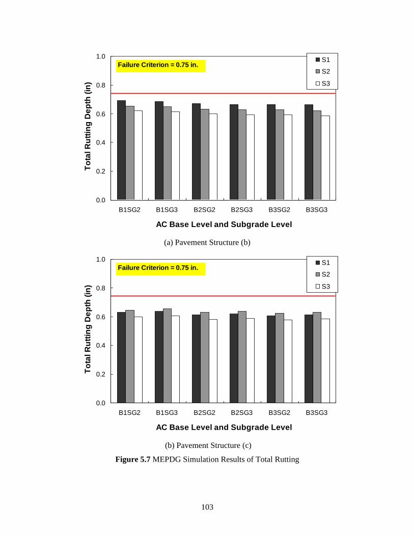
103

0.0

0.2

0.4

0.6

0.8

1.0



To

tal R

utt

ing

De

pth

(in

)

S1

S2

S3



0.0

0.2

0.4

0.6

0.8

1.0



To

tal R

utt

ing

De

pth

(in

)

S1

S2

S3



Figure 5.7 MEPDG Simulation Results of Total Rutting

104

Finally, figure 5.8 presents the predicted performance of IRI from each combination of

layer moduli. No evident performance sensitivity was observed among different input level

combinations of the base layer and subgrade layer, while pavement structure (c) presented the

effect of surface layer characteristics on overall pavement roughness.

For both pavement structures analyzed in this study, the performance variation related to

the stiffness of the subgrade layer was not significant for all type of distresses, although the

resilient modulus values used for the Level 2 and Level 3 differed by around 70 percent. Similar

results can also be found in several studies (Hoerner et al. 2007, McCracken et al. 2008, and Kim

et al. 2005). They reported that the resilient modulus of subgrade has minimal effect on the

pavement performance. Based on the observed analysis results herein and the research outcomes

presented in other studies, it can be concluded that the effect of the hierarchical subgrade

modulus input on the overall predicted pavement performance is not significant.

105

50

100

150

200

250



IRI (i

n/m

ile

)

S1

S2

S3

Failure Criterion = 172 in./mile


50

100

150

200

250



IRI (i

n/m

ile

)

S1

S2

S3

Failure Criterion = 172 in./mile


Figure 5.8 MEPDG Simulation Results of IRI

106

Chapter 6 Summary and Conclusions

The layer modulus database of various pavement materials used in Nebraska was

developed at all three hierarchical levels for a step-wise implementation of the new Mechanistic-

Empirical Pavement Design Guide (MEPDG). The database presented inputs of 20 HMA

mixtures, two native soils, and nine stabilized soils typically used in Nebraska pavements for use

with the MEPDG design-analysis software. Modulus values for each design level were then

applied to the MEPDG software to perform sensitivity analyses. The sensitivity analyses

investigated level-dependent performance predictions obtained from the MEPDG simulations of

typical Nebraska asphalt pavement structures. Based on the test results and analyses, the

following conclusions were drawn.

6.1 Conclusions

From the laboratory dynamic modulus test results of 20 HMA mixtures, variations in the

dynamic modulus values among the mixtures were found, even though these were the same

type of mixtures. This implies that mixture stiffness characteristics are related to properties

and proportioning of mixture constituents. Individual mixtures of the same mixture type were

produced with different blends of components.

When comparing dynamic modulus master curves among levels, a discrepancy was evident

between Level 1 (measured) master curves and Level 2 or 3 (predicted) master curves. The

level of discrepancy between curves was mixture-specific and generally larger at lower and

higher loading frequencies. Differences between Level 2 and Level 3 master curves were not

significant, which may be because Witczak’s predictive model was used for both levels.

Creep compliance test results for all 20 HMA mixtures presented similar observations with

dynamic modulus testing. Variations in creep compliance values were apparent among the

107

mixtures, even though they were the same type of mixtures. Comparison of creep compliance

results obtained from the Level 2 testing to the Level 3 estimation demonstrated a mixture-

specific discrepancy between the two levels.

The resilient modulus test was performed only for the two unbound soils, loess/till and

sandy silt. Testing difficulties were encountered in performing the resilient modulus test of

loess soil because of significant plastic deformation during the test. In addition to the two

native unbound soils tested for the Level 1 resilient modulus characterization, the resilient

modulus characteristics were also determined for the nine stabilized soils (loess, till, and

shale stabilized with hydrated lime, fly ash and cement kiln dust, respectively) that were

studied by Hensley et al. (2007) for a previous NDOR research project.

Resilient modulus test results for the Level 1 inputs clearly demonstrated that resilient

modulus of soils is stress-state dependent. The stress-dependent resilient modulus of soils

was characterized by identifying the three model parameters (k1, k2, k3) in the generalized

constitutive model. On the other hand, Level 2 and 3 resilient modulus inputs are stress-

independent values and therefore different from the Level 1 characterization.

MEPDG sensitivity analyses were conducted to evaluate the effects of using different design

input levels on MEPDG performance predictions of asphalt pavement structures. Sensitivity

analysis results conducted for typical full-depth flexible pavement structures showed

somewhat strong effects of design input levels. For the particular example case in this

research, pavement performance indicators, such as the longitudinal cracking, thermal

cracking, and rutting, were sensitively affected by the design inputs of the surface and/or

base layer. However, the performance variation related to the stiffness of the subgrade layer

was not significant for all type of distresses.

108

6.2 NDOR Implementation Plan

The primary focus of this research was to obtain the layer moduli of various asphalt types

currently used in Nebraska. This research has provided those moduli values, which will be

utilized in our current pavement design procedures. This research also provided valuable data

about the prediction models that are internal to the Mechanistic-Empirical Pavement Design

Guide (MEPDG) software. This data will be used for the future development of Nebraska’s

implementation of the Mechanistic-Empirical Design procedures.

109

References

AASHTO. 2008. “Mechanistic-Empirical Pavement Design Guide: A Manual of Practice,

Interim Edition.” American Association of State Highway and

Transportation Officials, Washington, D.C.

AASHTO. 2008. “Classification of Soils and Soil-Aggregate Mixtures for

Highway Construction Purposes.” AASHTO M 145: Standard Specifications for

Transportation and Methods of Sampling and Testing, 28th Edition, and Provisional

Standards, American Association of State Highway and Transportation Officials,

Washington, D.C.

AASHTO. 2008. “Particle Size Analysis of Soils.” AASHTO T 88-00: Standard

Specifications for Transportation and Methods of Sampling and Testing, 28th Edition,

and Provisional Standards, American Association of State Highway and Transportation

Officials, Washington, D.C.

AASHTO. 2008. “Determining the Liquid Limit of Soils.” AASHTO T 89-02: Standard

Specifications for Transportation and Methods of Sampling and Testing, 28th

Edition, and Provisional Standards, American Association of State Highway and


AASHTO. 2008. “Determining the Plastic Limit and Plasticity Index of Soils.”

AASHTO T 90-00: Standard Specifications for Transportation and Methods of Sampling

and Testing, 28th Edition, and Provisional Standards, American Association of State

Highway and Transportation Officials, Washington, D.C.

AASHTO. 2008. “Moisture-Density Relations of Soils Using a 5.5 lb Rammer

and a 12 in. Drop.” AASHTO T 99-01: Standard Specifications for Transportation and

Methods of Sampling and Testing, 28th Edition, and Provisional Standards, American

Association of State Highway and Transportation Officials, Washington, D.C.

AASHTO. 2008. “Specific Gravity of Soils.” AASHTO T 100-06: Standard Specifications for

Transportation and Methods of Sampling and Testing, 28th Edition, and

Provisional Standards, American Association of State Highway and Transportation


AASHTO. 2008. “Bulk Specific Gravity of Compacted Hot Mix Asphalt

Mixtures Using Saturated Surface-Dry Specimens.” AASHTO T 166-07: Standard

Specifications for Transportation and Methods of Sampling and Testing, 28th Edition,

and Provisional Standards, American Association of State Highway and Transportation


110

AASHTO. 2008. “Determining the Resilient Modulus of Soils and Aggregate Materials.”

AASHTO T 307-99: Standard Specifications for Transportation and Methods of Sampling

and Testing, 28th Edition, and Provisional Standards, American


AASHTO. 2008. “Determining the Creep Compliance and Strength of Hot-

Mix Asphalt (HMA) Using the Indirect Tensile Test Device.” AASHTO T 322-07:

Standard Specifications for Transportation and Methods of Sampling and Testing, 28th

Edition, and Provisional Standards, American Association of State Highway and


AASHTO. 2008. “Determining Dynamic Modulus of Hot-Mix Asphalt

Concrete Mixtures.” AASHTO TP 62-07, Standard Specifications for Transportation and

Methods of Sampling and Testing, 28th Edition, and Provisional Standards, American


Ali, O. 2005. “Evaluation of the Mechanistic Empirical Pavement Design Guide (NCHRP 1-

37A).” Report No. UR 3002.1, Research Report No. 216, National Research

Council Canada.

Andrei, D., M. W. Witczak, & M. W. Mirza. 2005. Development of Revised

Predictive Model for the Dynamic Complex Modulus of Asphalt Mixtures

(NCHRP 1-37A), University of Maryland, College Park, Maryland.

ASTM. 2007. “Standard Test Method for Particle-Size Analysis of Soils.” ASTM D422-6,

West Conshohocken, Pennsylvania.

Coree, B., H. Ceylan, and D. Harrington. 2005. “Implementing the Mechanistic-

Empirical Pavement Design Guide.” IHRB Project TR-509, Iowa Department of

Transportation, Iowa State University, Ames, IA.

Daniel, J. S., and G. R. Chehab. 2008. “Use of RAP Mixtures in Mechanistic Empirical

Pavement Design Guide.” Proc., Transportation Research Board 87th

Annual Meeting

(CD-ROM), National Research Council, Washington, D.C.

Fernando, E. G., J. Oh, and D. Ryu. 2007. “Phase I of M-EPDG Program

Implementation in Florida.” Research Report D04491/PR15281-1, Florida

Department of Transportation, Texas Transportation Institute, College Station, TX.

Flintsch, G. W., A. Loulizi, S. D. Diefenderfer, K. A. Galal, and B. K. Diefenderfer. 2007.

“Asphalt Materials Characterization in Support of Implementation of the

Proposed Mechanistic-Empirical Pavement Design Guide.” Research Report

VTRC 07-CR10, Virginia Department of Transportation.

111

Flintsch, G. W., A. Loulizi, S. D. Diefenderfer, B. K. Diefenderfer, and K. A. Galal. 2008.

“Asphalt Materials Characterization in Support of the Mechanistic-

Empirical Pavement Design Guide Implementation Efforts in Virginia.”

Transportation Research Record. 2057, Transportation Research Board, Washington,

D.C., 114-125.

Fonseca, O. A., and M. W. Witczak. 1996. “A Prediction Methodology for the

Dynamic Modulus of In-Place Aged Asphalt Mixtures.” Proc., The

Association of Asphalt Paving Technologists Annual Meeting, The

Association of Asphalt Paving Technologists, vol. 65, 532-572.

Hensley, T., J. Wayne, and C. Berryman. 2007. “Pozzolan Stabilized Subgrades.”

Research Report SPR-1(06) 578, Nebraska Department of Roads, Lincoln, NE.

Hoerner, T. E., K. A. Zimmerman, K. D. Smith, and L. A. Cooley. 2007. “Mechanistic-

Empirical Pavement Design Guide Implementation Plan.” Research Report

SD2005-01, South Dakota Department of Transportation, Pierre, SD.

Huang, Y. 1993. Pavement Analysis and Design. 2nd Edition. Pearson

Prentice Hall, Upper Saddle River, NJ.

Kesiraju, S., and H. Bahia. 2007. “Development of a Regional Pavement Performance

Database for the AASHTO Mechanistic – Empirical Pavement Design Guide:

Part 1: Sensitivity Analysis.” Research Report MRUTC 07-01, Wisconsin

Department of Transportation, University of Wisconsin, Madison, WI.

Khazanovich, L., C. Celauro, B. Chadbourn, J. Zollars, and S. Dai. 2006. “Evaluation

of the Subgrade Resilient Modulus Predictive Model for Use in the

MEPDG.” Proc., Transportation Research Board 85th

Annual Meeting (CD-ROM),

National Research Council, Washington, D.C.

Kim, S., H. Ceylan, and M. Heitzman. 2005. “Pavement Systems Using the

Mechanistic-Empirical Pavement Design Guide.” Proc., Mid-

Continent Transportation Research Symposium, Iowa State University, Ames, IA.

Kim, Y. R., M. King, and M. Momen. 2005. “Typical Dynamic Moduli for North

Carolina Asphalt Concrete Mixes.” Research Report FHWA/NC/2005-03, North Carolina

Department of Transportation, Raleigh, NC.

McCracken, J. K., J. M. Vandenbossche, and R. E. Asbahan. 2008. “Effect of the

MEPDG Hierarchal Levels on the Predicted Performance of a Jointed Plain

Concrete Pavement.” Proc., 9th International Conference on Concrete Pavements, San

Francisco, California.

112

Nazzal, M. D., L. N. Mohammad, and K. Gaspard. 2008. “Development of Resilient

Modulus Prediction Models for Louisiana Subgrade Soils.” Proc., Transportation

Research Board 87th

Annual Meeting, National Research Council, Washington, D.C.

National Cooperative Highway Research Program. (2004). “Guide for Mechanistic-Empirical

Design of New and Rehabilitated Pavement Structures.” NCHRP Project 1-37A,

National Research Council, Washington, D.C.

Pellinen T. K., M. W. Witczak. 2002. “Stress Dependent Master Curve Construction for

Dynamic (Complex) Modulus.” Journal of the Association of Asphalt Paving

Technologists, 71, 281-309.

Richardson, D., T. Petry, L. Ge, Y. P. Han, and S. M. Lusher. 2009. “Resilient Moduli of

Typical Missouri Soils and Unbound Granular Base Materials.” Research Report

RI06-001, Missouri Department of Transportation, Jefferson City, MO.

Schwartz, C. W. 2007. “Implementation of the NCHRP 1-37A Design Guide, Volume

1: Summary of Findings and Implementation Plan.” Research Report MDSHA

Project No. SP0077B41, Maryland State Highway Administration, Baltimore, MD.

Tashman, L. and M. A. Elangovan. 2007. “Dynamic Modulus Test – Laboratory

Investigation and Future Implementation in the State of Washington.” Research

Report WA-RD 704.1, Washington State Department of Transportation, Olympia, WA.

Uzan, J. 1985. “Characterization of Granular Materials.” Transportation Research

Record. 1022, Transportation Research Board, Washington, D.C., 52-59.

Velasquez, R., K. Hoegh, I. Yut, N. Funk, G. Cochram, M. Marasteanu, and

L. Khazanovich. 2009. “Implementation of the MEPDG for New and

Rehabilitated Pavement Structures for Design of Concrete and Asphalt Pavements in

Minnesota.” Research Report MN/RC 2009-06, Minnesota Department of Transportation,

St. Paul, MN.

Williams, R. C. 2007. “Testing Wisconsin Asphalt Mixtures for the AASHTO 2002

Mechanistic Design Procedure.” Research Report WHRP 07-06, Wisconsin

Department of Transportation, Madison, WI.

Witczak, M. W., and J. Bari, J. 2004. “Development of a Master Curve Database for Lime

Modified Asphalt Mixtures.” Arizona State University, Tempe, AZ.

113

Appendix A HMA Database for MEPDG

114

Project Number: RD 9-4(1012) Asphalt Cement

Name of Road: EMERSON TO WAKEFIELD NORTH Source: Flint Hills

Type of Asphalt Concrete: HRB (2008 yr) Grade: PG 58-28

Aggregate Gradation

Cumulative %

Retained 3/4 inch

Cumulative %

Retained 3/8 inch

Cumulative %

Retained #4 sieve

% Passing

#200 sieve

0 8.5 17.5 6

Dynamic Modulus (psi)

Temperature

(°F)

Frequency (Hz)

0.1 0.5 1 5 10 25

10 2543899.6 2660061.2 2782350.1 3080025.9 3207938.2 3300223.4

40 1291776.1 1516767.2 1728366.8 1969848.8 2148699.8 2257414.1

70 192506.7 295673.4 382967.3 680259.3 846756.6 1017114.1

100 50985.6 66159.2 83160.6 154296.8 192571.1 271091.7

130 36088.4 37897.1 41584.8 59512.5 70513.5 89270.5

Binder Properties

Superpave binder data (at Short Term Aging - RTFO)

Temperature

(°F) At 70 (°F) At 85 (°F) At 100 (°F)

Properties G*(Pa) Delta (°) G*(Pa) Delta (°) G*(Pa) Delta (°)

1122000 64.37 274800 69.46 72530 73.5

Volumetric Properties

Effective Binder

Content (%)

Air Voids

(%)

Total Unit

Weight (pcf)

Maximum Specific

Gravity

10.5 4.2 144.9 2.424

Thermal Cracking

Creep Compliance (1/psi)

Loading Time (sec) at Medium Temperature (14°F) with Level 2

1 2 5 10 20 50 100

1.07E-07 2.80E-07 3.72E-07 4.36E-07 5.09E-07 6.04E-07 7.40E-07

Average tensile strength at 14 (°F) 439.05

115

Project Number: RD 81-2(1037) Asphalt Cement

Name of Road: IN YORK Source: Flint Hills


Aggregate Gradation

Cumulative %

Retained 3/4 inch

Cumulative %

Retained 3/8 inch

Cumulative %

Retained #4 sieve

% Passing

#200 sieve

0 3.8 14.6 7.7


Temperature

(°F)

Frequency (Hz)

0.1 0.5 1 5 10 25

10 1831067.3 1951430.7 2094582.9 2339753.9 2479891.6 2502839.6

40 886394.9 1001843.0 1177350.6 1557480.7 1692684.9 1838489.7

70 150607.4 224404.4 302152.0 565929.2 691838.3 818614.8

100 42802.7 50973.8 66487.3 125697.1 160454.5 231657.4

130 32271.7 31103.6 32572.1 44036.8 47692.5 63445.0

Binder Properties


Temperature

(°F) At 70 (°F) At 85 (°F) At 100 (°F)


1330000 63.12 325400 68.01 82040 72.24


Effective Binder

Content (%)

Air Voids

(%)

Total Unit

Weight (pcf)

Maximum Specific

Gravity

11.2 4.0 145.0 2.420

Thermal Cracking



1 2 5 10 20 50 100

7.31E-08 2.18E-07 3.09E-07 3.87E-07 4.54E-07 6.37E-07 8.25E-07


116

Project Number: STP 14-4(110) Asphalt Cement

Name of Road: ELGIN TO US-20 & PLAINVIEW WEST ON US-20 Source: JEBRO


Aggregate Gradation

Cumulative %

Retained 3/4 inch

Cumulative %

Retained 3/8 inch

Cumulative %

Retained #4 sieve

% Passing

#200 sieve

0 4.5 11.8 5.9


Temperature

(°F)

Frequency (Hz)

0.1 0.5 1 5 10 25

10 2190029.5 2291099.6 2493332.2 2909207.5 2940971.4 3034239.1

40 912895.3 1077580.9 1241729.3 1632184.5 1803570.8 1955574.8

70 153183.6 210606.4 281419.8 531234.3 651579.7 800466.1

100 37573.6 42036.7 56476.7 108609.1 142988.2 205805.3

130 31385.8 32022.6 32662.8 48260.0 54281.0 65851.9

Binder Properties


Temperature

(°F) At 70 (°F) At 85 (°F) At 100 (°F)


1311000 59.37 328500 65.59 88560 69.92


Effective Binder

Content (%)

Air Voids

(%)

Total Unit

Weight (pcf)

Maximum Specific

Gravity

11.8 3.9 144.9 2.415

Thermal Cracking



1 2 5 10 20 50 100

2.71E-07 4.75E-07 5.84E-07 6.59E-07 7.63E-07 9.35E-07 1.12E-06


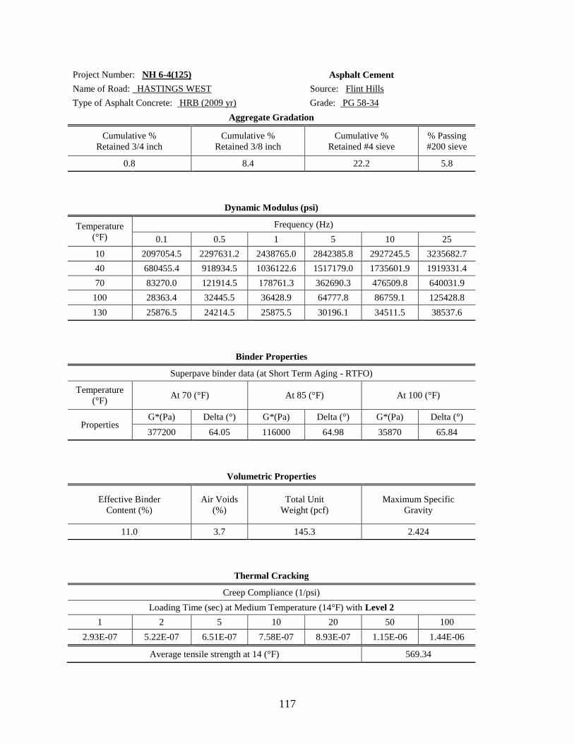
117

Project Number: NH 6-4(125) Asphalt Cement

Name of Road: HASTINGS WEST Source: Flint Hills


Aggregate Gradation

Cumulative %

Retained 3/4 inch

Cumulative %

Retained 3/8 inch

Cumulative %

Retained #4 sieve

% Passing

#200 sieve

0.8 8.4 22.2 5.8


Temperature

(°F)

Frequency (Hz)

0.1 0.5 1 5 10 25

10 2097054.5 2297631.2 2438765.0 2842385.8 2927245.5 3235682.7

40 680455.4 918934.5 1036122.6 1517179.0 1735601.9 1919331.4

70 83270.0 121914.5 178761.3 362690.3 476509.8 640031.9

100 28363.4 32445.5 36428.9 64777.8 86759.1 125428.8

130 25876.5 24214.5 25875.5 30196.1 34511.5 38537.6

Binder Properties


Temperature

(°F) At 70 (°F) At 85 (°F) At 100 (°F)


377200 64.05 116000 64.98 35870 65.84


Effective Binder

Content (%)

Air Voids

(%)

Total Unit

Weight (pcf)

Maximum Specific

Gravity

11.0 3.7 145.3 2.424

Thermal Cracking



1 2 5 10 20 50 100

2.93E-07 5.22E-07 6.51E-07 7.58E-07 8.93E-07 1.15E-06 1.44E-06


118

Project Number: STPD 6-6(156) Asphalt Cement

Name of Road: DORCHESTER TO MILFORD Source: Flint Hills

Type of Asphalt Concrete: SPL (2008 yr) Grade: PG 58-28

Aggregate Gradation

Cumulative %

Retained 3/4 inch

Cumulative %

Retained 3/8 inch

Cumulative %

Retained #4 sieve

% Passing

#200 sieve

1.1 13.6 27.1 7.5


Temperature

(°F)

Frequency (Hz)

0.1 0.5 1 5 10 25

10 2656874.4 2728711.3 2880849.8 3146278.7 3303297.2 3271087.3

40 1101444.3 1274602.1 1445819.5 1869871.5 2008415.8 2206527.7

70 177780.0 307653.3 413332.0 735147.6 865229.5 997621.2

100 53737.8 60183.6 80531.6 181242.3 208254.7 286939.4

130 37725.3 39297.5 53771.4 59228.5 59300.9 74802.9

Binder Properties


Temperature

(°F) At 70 (°F) At 85 (°F) At 100 (°F)


1373000 63.17 340200 67.89 85470 72.44


Effective Binder

Content (%)

Air Voids

(%)

Total Unit

Weight (pcf)

Maximum Specific

Gravity

9.5 3.8 147.0 2.449

Thermal Cracking



1 2 5 10 20 50 100

1.26E-07 2.25E-07 2.65E-07 2.97E-07 3.37E-07 4.07E-07 4.77E-07


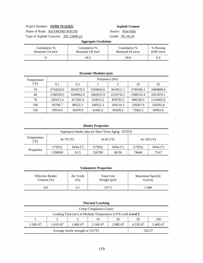
119

Project Number: STPD-79-2(102) Asphalt Cement

Name of Road: RAYMOND SOUTH Source: Flint Hills


Aggregate Gradation

Cumulative %

Retained 3/4 inch

Cumulative %

Retained 3/8 inch

Cumulative %

Retained #4 sieve

% Passing

#200 sieve

0 18.5 30.8 6.9


Temperature

(°F)

Frequency (Hz)

0.1 0.5 1 5 10 25

10 2734224.0 3034270.5 3294642.6 3619511.1 3749186.1 3484809.0

40 1340550.5 1649962.9 1862052.9 2254756.1 2386535.4 2451876.1

70 245471.4 417205.4 524915.2 850792.2 966330.5 1156902.8

100 50798.7 88522.3 108551.3 204110.3 258207.9 356502.8

130 29918.9 36478.9 43402.2 66509.3 72062.5 60003.6

Binder Properties


Temperature

(°F) At 70 (°F) At 85 (°F) At 100 (°F)


1298000 63.5 326700 68.56 74640 73.67


Effective Binder

Content (%)

Air Voids

(%)

Total Unit

Weight (pcf)

Maximum Specific

Gravity

8.6 4.1 147.5 2.466

Thermal Cracking



1 2 5 10 20 50 100

1.50E-07 1.61E-07 1.86E-07 2.14E-07 2.98E-07 4.22E-07 5.46E-07


120

Project Number: STP-91-3(107) Asphalt Cement

Name of Road: TAYLOR EAST Source: Flint Hills


Aggregate Gradation

Cumulative %

Retained 3/4 inch

Cumulative %

Retained 3/8 inch

Cumulative %

Retained #4 sieve

% Passing

#200 sieve

0 16.6 28.2 5.5


Temperature

(°F)

Frequency (Hz)

0.1 0.5 1 5 10 25

10 1856757.2 1964578.5 2088753.4 2424598.8 2514705.4 2557477.4

40 786061.0 930340.6 1083982.7 1502493.0 1656655.9 1797114.1

70 149985.3 218513.3 290692.9 537784.9 675369.3 869362.4

100 51053.7 58510.2 65429.8 122193.1 152756.4 217889.8

130 35465.4 36812.2 37173.8 48469.5 58175.1 70915.8

Binder Properties


Temperature

(°F) At 70 (°F) At 85 (°F) At 100 (°F)


469500 64.03 139800 64.74 41900 65.29


Effective Binder

Content (%)

Air Voids

(%)

Total Unit

Weight (pcf)

Maximum Specific

Gravity

9.4 4.3 145.8 2.443

Thermal Cracking



1 2 5 10 20 50 100

2.91E-07 4.61E-07 5.73E-07 6.67E-07 7.82E-07 9.91E-07 1.22E-06


121

Project Number: NH-80-9(832),(825),(827) Asphalt Cement

Name of Road: GREENWOOD TO MAHONEY Source: MONARCH


Aggregate Gradation

Cumulative %

Retained 3/4 inch

Cumulative %

Retained 3/8 inch

Cumulative %

Retained #4 sieve

% Passing

#200 sieve

1.5 14.4 23.1 7.7


Temperature

(°F)

Frequency (Hz)

0.1 0.5 1 5 10 25

10 2591924.9 2691213.4 2823077.4 3093657.7 3190453.1 3236438.5

40 1300154.1 1429971.3 1581567.0 1968816.8 2094123.0 2261920.0

70 288516.3 391251.3 494634.2 824001.9 970045.9 1121245.9

100 68716.7 90706.1 111405.9 232127.5 296792.1 396367.0

130 32810.6 34252.6 39033.0 64506.0 79339.8 101739.2

Binder Properties


Temperature

(°F) At 70 (°F) At 85 (°F) At 100 (°F)


1415000 56.7 440600 61.5 130500 63.21


Effective Binder

Content (%)

Air Voids

(%)

Total Unit

Weight (pcf)

Maximum Specific

Gravity

9.5 4.1 146.8 2.454

Thermal Cracking



1 2 5 10 20 50 100

1.98E-07 2.75E-07 3.05E-07 3.31E-07 3.69E-07 4.42E-07 5.23E-07


122

Project Number: RD-81-2 (1037) Asphalt Cement

Name of Road: IN YORK Source: Flint Hills

Type of Asphalt Concrete: SP4 (0.375) (2008 yr) Grade: PG 64-28

Aggregate Gradation

Cumulative %

Retained 3/4 inch

Cumulative %

Retained 3/8 inch

Cumulative %

Retained #4 sieve

% Passing

#200 sieve

0.1 3.5 17.1 6.9


Temperature

(°F)

Frequency (Hz)

0.1 0.5 1 5 10 25

10 2568877.8 2683453.8 2862536.0 3204519.3 3323408.8 3416495.9

40 1054986.6 1270094.0 1481885.4 1961818.4 2175465.3 2453835.1

70 163956.2 236487.0 312133.9 604859.0 736558.3 912207.1

100 43222.9 54299.7 70769.1 130867.4 175560.7 248213.6

130 42989.5 43793.7 42421.6 58221.0 64192.8 77575.5

Binder Properties


Temperature

(°F) At 70 (°F) At 85 (°F) At 100 (°F)


1270000 59.27 354300 63.47 103600 65.19


Effective Binder

Content (%)

Air Voids

(%)

Total Unit

Weight (pcf)

Maximum Specific

Gravity

10.4 3.9 145.6 2.430

Thermal Cracking



1 2 5 10 20 50 100

1.85E-07 3.36E-07 4.08E-07 4.65E-07 5.32E-07 6.46E-07 7.62E-07


123

Project Number: RD-9-4(1012) Asphalt Cement

Name of Road: EMERSON TO WAKEFIELD Source: Flint Hills


Aggregate Gradation

Cumulative %

Retained 3/4 inch

Cumulative %

Retained 3/8 inch

Cumulative %

Retained #4 sieve

% Passing

#200 sieve

0 4.7 15.9 4.6


Temperature

(°F)

Frequency (Hz)

0.1 0.5 1 5 10 25

10 1828347.1 2135366.8 2286956.6 2581680.4 2632575.3 2626224.0

40 691676.3 947599.5 1112873.2 1484841.0 1593921.3 1683507.7

70 109317.9 176762.3 235497.8 440129.9 549142.3 684896.4

100 33200.5 49927.9 58642.9 102503.8 123459.6 177119.3

130 28620.4 32868.0 35891.3 44994.1 53763.6 59647.5

Binder Properties


Temperature

(°F) At 70 (°F) At 85 (°F) At 100 (°F)


1184000 61.57 294200 65.08 86920 66.06


Effective Binder

Content (%)

Air Voids

(%)

Total Unit

Weight (pcf)

Maximum Specific

Gravity

11.5 4.0 144.3 2.409

Thermal Cracking



1 2 5 10 20 50 100

1.95E-07 3.47E-07 4.46E-07 5.05E-07 5.95E-07 7.49E-07 8.90E-07


124

Project Number: NH-6-4(125) Asphalt Cement

Name of Road: HASTINGS WEST Source: Flint Hills


Aggregate Gradation

Cumulative %

Retained 3/4 inch

Cumulative %

Retained 3/8 inch

Cumulative %

Retained #4 sieve

% Passing

#200 sieve

0 3.6 12.8 5.4


Temperature

(°F)

Frequency (Hz)

0.1 0.5 1 5 10 25

10 2736367.7 2960234.9 3079546.3 3418065.4 3327987.5 3657522.8

40 1170982.4 1427465.3 1538830.7 2040142.7 2230419.7 2404839.5

70 146071.5 221605.9 308553.6 602689.7 758221.1 956026.3

100 42116.1 49160.4 66077.7 118184.4 157125.8 230277.6

130 30583.4 30643.2 32494.8 45625.8 52408.7 69506.6

Binder Properties


Temperature

(°F) At 70 (°F) At 85 (°F) At 100 (°F)


1124000 62.74 281800 65.2 79630 66.05


Effective Binder

Content (%)

Air Voids

(%)

Total Unit

Weight (pcf)

Maximum Specific

Gravity

11.1 3.8 145.5 2.423

Thermal Cracking



1 2 5 10 20 50 100

1.04E-07 1.90E-07 2.32E-07 2.67E-07 3.16E-07 4.09E-07 5.23E-07


125


Name of Road: WALLACE SOUTH Source: JEBRO


Aggregate Gradation

Cumulative %

Retained 3/4 inch

Cumulative %

Retained 3/8 inch

Cumulative %

Retained #4 sieve

% Passing

#200 sieve

0 1.7 12.9 7.7


Temperature

(°F)

Frequency (Hz)

0.1 0.5 1 5 10 25

10 2352905.0 2504044.6 2636020.4 2952482.2 3096571.9 3276636.2

40 1106325.1 1282804.9 1466726.7 1929211.2 2106181.2 2329040.7

70 164030.8 240708.0 326227.2 586287.3 728898.5 930941.0

100 43697.7 56565.6 68178.8 135264.2 177667.1 256495.8

130 27723.6 27179.6 30738.6 43616.6 50841.8 66251.9

Binder Properties


Temperature

(°F) At 70 (°F) At 85 (°F) At 100 (°F)


1162000 62.51 291400 65.51 82730 67.31


Effective Binder

Content (%)

Air Voids

(%)

Total Unit

Weight (pcf)

Maximum Specific

Gravity

11.5 4.2 144.5 2.416

Thermal Cracking



1 2 5 10 20 50 100

2.19E-07 3.23E-07 3.90E-07 4.51E-07 5.35E-07 7.05E-07 8.99E-07


126

Project Number: PEP-183-1 (1020) Asphalt Cement

Name of Road: Source: MONARCH


Aggregate Gradation

Cumulative %

Retained 3/4 inch

Cumulative %

Retained 3/8 inch

Cumulative %

Retained #4 sieve

% Passing

#200 sieve

0 11.1 24.9 4.4


Temperature

(°F)

Frequency (Hz)

0.1 0.5 1 5 10 25

10 2214166.3 2623301.7 2697566.0 2573689.2 2810799.0 2434479.3

40 1019577.6 1338239.3 1462163.6 1903738.1 1940090.5 1796865.8

70 237148.5 353805.8 457334.5 754418.9 865924.8 1017322.7

100 62104.4 92709.1 120265.6 208645.6 250617.9 338105.2

130 35944.7 45470.7 50658.2 71624.6 82675.7 103470.4

Binder Properties


Temperature

(°F) At 70 (°F) At 85 (°F) At 100 (°F)


1176000 58.15 379200 63.43 126300 65.04


Effective Binder

Content (%)

Air Voids

(%)

Total Unit

Weight (pcf)

Maximum Specific

Gravity

11.2 4.10 146.0 2.440

Thermal Cracking



1 2 5 10 20 50 100

1.56E-07 2.70E-07 3.15E-07 3.49E-07 3.93E-07 4.71E-07 5.49E-07


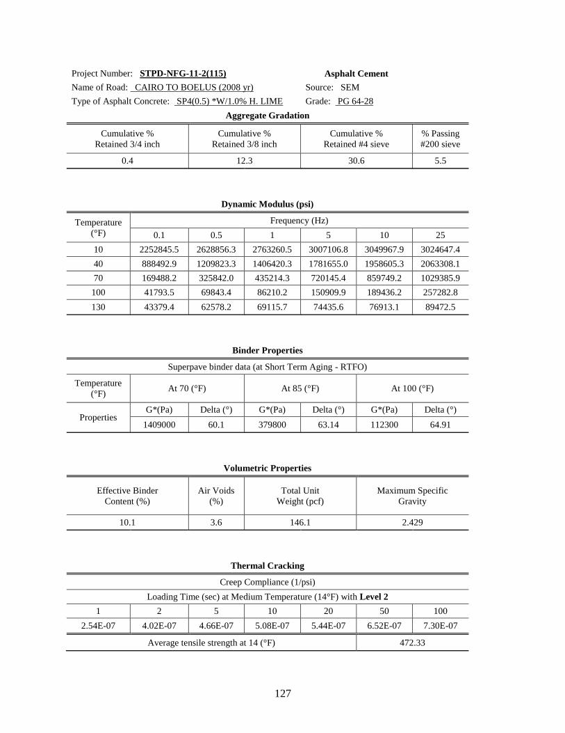
127

Project Number: STPD-NFG-11-2(115) Asphalt Cement

Name of Road: CAIRO TO BOELUS (2008 yr) Source: SEM

Type of Asphalt Concrete: SP4(0.5) *W/1.0% H. LIME Grade: PG 64-28

Aggregate Gradation

Cumulative %

Retained 3/4 inch

Cumulative %

Retained 3/8 inch

Cumulative %

Retained #4 sieve

% Passing

#200 sieve

0.4 12.3 30.6 5.5


Temperature

(°F)

Frequency (Hz)

0.1 0.5 1 5 10 25

10 2252845.5 2628856.3 2763260.5 3007106.8 3049967.9 3024647.4

40 888492.9 1209823.3 1406420.3 1781655.0 1958605.3 2063308.1

70 169488.2 325842.0 435214.3 720145.4 859749.2 1029385.9

100 41793.5 69843.4 86210.2 150909.9 189436.2 257282.8

130 43379.4 62578.2 69115.7 74435.6 76913.1 89472.5

Binder Properties


Temperature

(°F) At 70 (°F) At 85 (°F) At 100 (°F)


1409000 60.1 379800 63.14 112300 64.91


Effective Binder

Content (%)

Air Voids

(%)

Total Unit

Weight (pcf)

Maximum Specific

Gravity

10.1 3.6 146.1 2.429

Thermal Cracking



1 2 5 10 20 50 100

2.54E-07 4.02E-07 4.66E-07 5.08E-07 5.44E-07 6.52E-07 7.30E-07


128


Name of Road: CHAMBERS JCT. NORTH Source: JEBRO


Aggregate Gradation

Cumulative %

Retained 3/4 inch

Cumulative %

Retained 3/8 inch

Cumulative %

Retained #4 sieve

% Passing

#200 sieve

0.2 9.3 17 5.7


Temperature

(°F)

Frequency (Hz)

0.1 0.5 1 5 10 25

10 2853206.8 2957393.6 3123457.3 3522600.2 3839701.8 3932635.5

40 1286461.6 1488620.8 1703854.1 2217252.3 2437694.5 2587352.8

70 204302.9 287386.3 395405.7 723874.8 900989.0 1092335.5

100 59080.4 73431.9 87097.5 174140.5 234282.6 322478.9

130 36756.5 34528.4 38174.1 51805.8 62725.5 83985.8

Binder Properties


Temperature

(°F) At 70 (°F) At 85 (°F) At 100 (°F)


1068000 63.14 284400 65.63 78250 67.59


Effective Binder

Content (%)

Air Voids

(%)

Total Unit

Weight (pcf)

Maximum Specific

Gravity

10.3 3.92 145.7 2.430

Thermal Cracking



1 2 5 10 20 50 100

2.78E-07 4.03E-07 4.70E-07 5.23E-07 5.86E-07 7.00E-07 8.24E-07


129


Name of Road: THEDFORD SOUTH Source: JEBRO

Type of Asphalt Concrete: SP4(0.5) (2009 yr) Grade: PG 64-28

Aggregate Gradation

Cumulative %

Retained 3/4 inch

Cumulative %

Retained 3/8 inch

Cumulative %

Retained #4 sieve

% Passing

#200 sieve

0 8.9 30.9 5


Temperature

(°F)

Frequency (Hz)

0.1 0.5 1 5 10 25

10 2615108.1 2711784.6 2886458.5 3195422.2 3358592.5 3786092.9

40 1021748.0 1192144.1 1364688.5 1799610.7 1992517.1 2319529.1

70 169663.7 240858.1 330839.8 589823.6 738174.2 909841.2

100 39871.3 52045.1 63820.6 136974.2 183080.9 258038.8

130 26576.4 28011.0 31581.6 43472.8 52610.9 68886.0

Binder Properties


Temperature

(°F) At 70 (°F) At 85 (°F) At 100 (°F)


1124000 62.74 281800 65.2 79630 66.05


Effective Binder

Content (%)

Air Voids

(%)

Total Unit

Weight (pcf)

Maximum Specific

Gravity

10.4 4.2 145.1 2.429

Thermal Cracking



1 2 5 10 20 50 100

2.47E-07 4.52E-07 5.63E-07 6.50E-07 7.55E-07 9.43E-07 1.14E-06


130


Name of Road: FORT STR. SOUTH, OMAHA Source: Flint Hills


Aggregate Gradation

Cumulative %

Retained 3/4 inch

Cumulative %

Retained 3/8 inch

Cumulative %

Retained #4 sieve

% Passing

#200 sieve

0 10.5 24.1 6.1


Temperature

(°F)

Frequency (Hz)

0.1 0.5 1 5 10 25

10 3063296.6 3169743.8 3415507.2 3540164.8 3814552.6 3995832.1

40 1828143.5 1842210.1 2024905.9 2446564.4 2640186.7 2791958.1

70 489704.5 625164.8 755084.5 1119519.9 1288385.3 1468226.7

100 97661.3 139433.3 185838.4 352278.5 438929.3 555331.5

130 55786.4 63579.1 71412.4 115612.1 142841.2 182549.4

Binder Properties


Temperature

(°F) At 70 (°F) At 85 (°F) At 100 (°F)


1410000 60.12 363000 62.98 113500 62.9


Effective Binder

Content (%)

Air Voids

(%)

Total Unit

Weight (pcf)

Maximum Specific

Gravity

9.7 3.9 146.8 2.448

Thermal Cracking



1 2 5 10 20 50 100

7.92E-08 1.38E-07 1.52E-07 1.63E-07 1.73E-07 1.89E-07 2.02E-07


131

Project Number: STPD-6-7(178) Asphalt Cement

Name of Road: GREENWOOD TO ASHLAND Source: JEBRO / Flint Hills


Aggregate Gradation

Cumulative %

Retained 3/4 inch

Cumulative %

Retained 3/8 inch

Cumulative %

Retained #4 sieve

% Passing

#200 sieve

1 10.1 20.4 6.8


Temperature

(°F)

Frequency (Hz)

0.1 0.5 1 5 10 25

10 2781317.9 2670536.5 3003834.4 3188212.0 3221113.8 3523836.0

40 1253042.1 1417307.3 1611422.4 2002855.3 2165463.3 2264449.0

70 260805.5 357472.6 462744.5 800013.9 932103.0 1102407.6

100 75315.6 93470.5 126910.7 230936.1 291956.4 385186.9

130 35212.4 40221.6 46524.3 68718.8 86644.4 112588.8

Binder Properties


Temperature

(°F) At 70 (°F) At 85 (°F) At 100 (°F)


1630000 59.8 377900 64.55 105800 66.03


Effective Binder

Content (%)

Air Voids

(%)

Total Unit

Weight (pcf)

Maximum Specific

Gravity

9.6 3.9 146.3 2.441

Thermal Cracking



1 2 5 10 20 50 100

2.25E-07 3.53E-07 3.92E-07 4.25E-07 4.44E-07 5.34E-07 5.78E-07


132


Name of Road: Lincoln South Source: Flint Hills


Aggregate Gradation

Cumulative %

Retained 3/4 inch

Cumulative %

Retained 3/8 inch

Cumulative %

Retained #4 sieve

% Passing

#200 sieve

0 6.2 22.3 3.8


Temperature

(°F)

Frequency (Hz)

0.1 0.5 1 5 10 25

10 2878547.1 2876997.0 2959608.0 3076199.5 3072403.4 3639388.4

40 1144281.8 1327891.8 1515637.5 1978565.4 2105509.7 2294792.5

70 242589.6 326246.5 420104.8 726675.8 882497.3 1046170.7

100 72683.9 90038.8 116725.6 208464.8 269761.7 360267.7

130 40969.7 42019.7 50828.8 78592.3 87908.1 108862.1

Binder Properties


Temperature

(°F) At 70 (°F) At 85 (°F) At 100 (°F)


1178000 62.3 293200 65.86 83730 67.45


Effective Binder

Content (%)

Air Voids

(%)

Total Unit

Weight (pcf)

Maximum Specific

Gravity

9.6 4.10 147.5 2.464

Thermal Cracking



1 2 5 10 20 50 100

7.23E-08 1.85E-07 2.36E-07 2.78E-07 3.32E-07 4.19E-07 4.84E-07


133

Project Number: IM-80-6(97) Asphalt Cement

Name of Road: WOOD RIVER TO GRAND ISLAND Source: Flint Hills


Aggregate Gradation

Cumulative %

Retained 3/4 inch

Cumulative %

Retained 3/8 inch

Cumulative %

Retained #4 sieve

% Passing

#200 sieve

0 8.8 19.5 5.4


Temperature

(°F)

Frequency (Hz)

0.1 0.5 1 5 10 25

10 3055089.1 3031140.5 3137813.7 3534049.5 3526444.1 3805294.2

40 1562122.9 1773741.2 1984390.8 2529887.1 2687549.3 2891389.6

70 283628.6 408648.4 543788.9 927070.5 1140891.9 1358296.2

100 66338.3 83353.9 105174.6 218045.9 282249.8 391417.8

130 36009.2 37474.8 43851.6 67281.5 82205.4 106902.6

Binder Properties


Temperature

(°F) At 70 (°F) At 85 (°F) At 100 (°F)


1332000 61.1 337300 63.4 101400 63.76


Effective Binder

Content (%)

Air Voids

(%)

Total Unit

Weight (pcf)

Maximum Specific

Gravity

10.7 3.7 145.8 2.425

Thermal Cracking



1 2 5 10 20 50 100

7.81E-08 1.39E-07 1.63E-07 1.82E-07 2.00E-07 2.43E-07 2.83E-07


134

Appendix B Soils Database for MEPDG

135

Resil

ien

t M

od

ulu

s T

esti

ng

- A

AS

HT

O T

30

7-9

9S

am

ple

's I

D:

OM

C C

ase #

1

So

il T

yp

e:

Lo

ess-T

ill

Co

mp

acte

d M

ois

ture

Co

nte

nt

(%):

19.1

0

Max.

Dry

Den

sit

y (

pcf)

:104.0

Fin

al S

am

ple

Dia

mete

r (i

n):

3.9

9L

iqu

id L

imit

:40

Mo

istu

re C

on

ten

t (%

):20.3

Fin

al S

am

ple

Heig

ht

(in

):8.0

3P

lasti

cit

y I

nd

ex:

21

Weig

ht

of

Wet

So

il (

lb)

7.2

6F

inal S

am

ple

Wet

Weig

ht

(lb

):7.2

5

Init

ial S

am

ple

Dia

mete

r (i

n):

3.9

4k1:

453.9

88

Init

ial S

am

ple

Heig

ht

(in

):8.0

7k2:

0.6

96

Init

ial S

am

ple

Are

a (

in2):

12.2

k3:

-5.8

08

Sam

ple

Vo

lum

e (

in3):

98.3

Seq

.

Co

nfi

ne

str

ess

(psi)

No

min

al

Maxi

mu

m

Axi

al

Str

ess

(Scy

clic)

(psi)

Actu

al

Ap

plied

Max.

Axi

al

Lo

ad

(P

max)

(lb

)

Actu

al

Ap

plied

Cy

clic

Lo

ad

(Pcy

clic)

(lb

)

Actu

al

Ap

plied

Co

nta

ct

Lo

ad

(Pco

nta

ct)

(lb

)

Actu

al

Ap

plied

Max.

Axi

al

Str

ess

(Sm

ax)

(psi)

Actu

al

Ap

plied

Cy

clic

Str

ess

(Scy

clic)

(psi)

Actu

al

Ap

plied

Co

nta

ct

Str

ess

(Sco

nta

ct)

(p

si)

Reco

v.

Def.

LV

DT

#1

read

ing

(in

)

Reco

v.

Def.

LV

DT

#2

read

ing

(in

)

Av

era

ge

Reco

v.

Def.

LV

DT

1 a

nd

2

read

ing

(in

)

Resilie

nt

Str

ain

(in

/in

)

Resilen

t

Mo

du

lus

(psi)

16.0

1.8

28.8

26.5

2.2

2.2

2.0

0.2

0.0

026

0.0

026

0.0

026

0.0

00317

6272.2

26.0

3.6

52.8

47.4

5.4

3.9

3.4

0.5

0.0

061

0.0

061

0.0

061

0.0

00751

4587.9

36.0

5.4

77.6

69.9

7.6

5.7

5.1

0.6

0.0

120

0.0

120

0.0

120

0.0

01488

3432.1

46.0

7.2

101.4

92.2

9.2

7.6

6.8

0.8

0.0

191

0.0

191

0.0

191

0.0

02366

2875.5

56.0

9.0

126.1

116.2

9.9

9.5

8.7

0.8

0.0

260

0.0

260

0.0

260

0.0

03224

2706.1

64.0

1.8

27.2

25.2

2.0

2.1

1.9

0.2

0.0

033

0.0

033

0.0

033

0.0

00407

4654.3

74.0

3.6

51.3

46.3

4.9

3.8

3.4

0.4

0.0

086

0.0

086

0.0

086

0.0

01066

3189.2

84.0

5.4

76.0

70.1

5.8

5.8

5.3

0.5

0.0

156

0.0

156

0.0

156

0.0

01934

2734.1

94.0

7.2

100.3

92.6

7.6

7.6

7.0

0.6

0.0

231

0.0

231

0.0

231

0.0

02861

2443.2

10

4.0

9.0

124.5

115.3

9.2

9.5

8.7

0.8

0.0

298

0.0

298

0.0

298

0.0

03695

2359.0

11

2.0

1.8

25.6

23.6

2.0

1.9

1.8

0.2

0.0

043

0.0

043

0.0

043

0.0

00532

3347.3

12

2.0

3.6

50.1

45.2

4.9

3.7

3.3

0.4

0.0

109

0.0

109

0.0

109

0.0

01356

2434.4

13

2.0

5.4

74.2

69.0

5.2

5.7

5.2

0.4

0.0

196

0.0

196

0.0

196

0.0

02432

2157.2

14

2.0

7.2

98.5

92.8

5.6

7.6

7.2

0.5

0.0

281

0.0

281

0.0

281

0.0

03483

2057.0

15

2.0

9.0

122.7

116.0

6.7

9.5

9.0

0.6

0.0

353

0.0

354

0.0

353

0.0

04378

2049.7

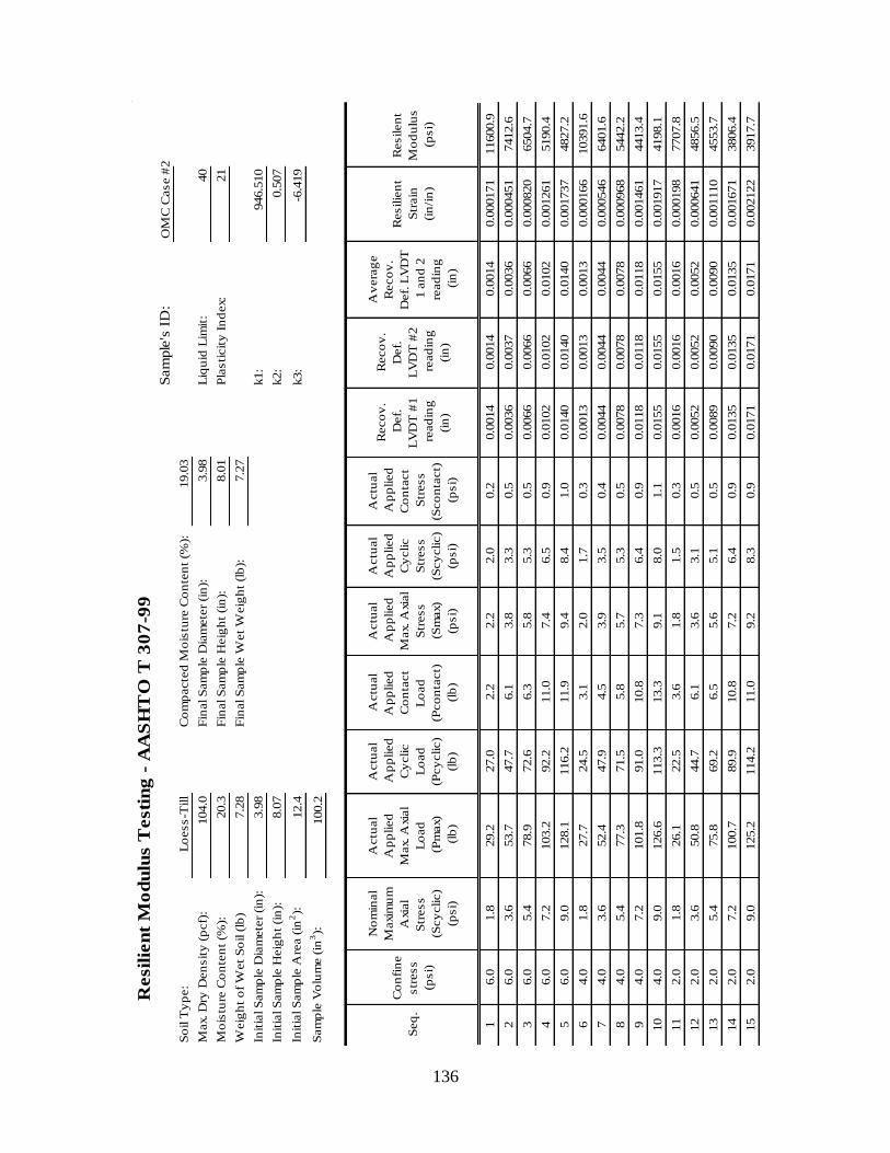
136

Resil

ien

t M

od

ulu

s T

esti

ng

- A

AS

HT

O T

30

7-9

9S

am

ple

's I

D:

OM

C C

ase #

2

So

il T

yp

e:

Lo

ess-T

ill

Co

mp

acte

d M

ois

ture

Co

nte

nt

(%):

19.0

3

Max.

Dry

Den

sit

y (

pcf)

:104.0

Fin

al S

am

ple

Dia

mete

r (i

n):

3.9

8L

iqu

id L

imit

:40

Mo

istu

re C

on

ten

t (%

):20.3

Fin

al S

am

ple

Heig

ht

(in

):8.0

1P

lasti

cit

y I

nd

ex:

21

Weig

ht

of

Wet

So

il (

lb)

7.2

8F

inal S

am

ple

Wet

Weig

ht

(lb

):7.2

7

Init

ial S

am

ple

Dia

mete

r (i

n):

3.9

8k1:

946.5

10

Init

ial S

am

ple

Heig

ht

(in

):8.0

7k2:

0.5

07

Init

ial S

am

ple

Are

a (

in2):

12.4

k3:

-6.4

19

Sam

ple

Vo

lum

e (

in3):

100.2

Seq

.

Co

nfi

ne

str

ess

(psi)

No

min

al

Maxi

mu

m

Axi

al

Str

ess

(Scy

clic)

(psi)

Actu

al

Ap

plied

Max.

Axi

al

Lo

ad

(P

max)

(lb

)

Actu

al

Ap

plied

Cy

clic

Lo

ad

(Pcy

clic)

(lb

)

Actu

al

Ap

plied

Co

nta

ct

Lo

ad

(Pco

nta

ct)

(lb

)

Actu

al

Ap

plied

Max.

Axi

al

Str

ess

(Sm

ax)

(psi)

Actu

al

Ap

plied

Cy

clic

Str

ess

(Scy

clic)

(psi)

Actu

al

Ap

plied

Co

nta

ct

Str

ess

(Sco

nta

ct)

(p

si)

Reco

v.

Def.

LV

DT

#1

read

ing

(in

)

Reco

v.

Def.

LV

DT

#2

read

ing

(in

)

Av

era

ge

Reco

v.

Def.

LV

DT

1 a

nd

2

read

ing

(in

)

Resilie

nt

Str

ain

(in

/in

)

Resilen

t

Mo

du

lus

(psi)

16.0

1.8

29.2

27.0

2.2

2.2

2.0

0.2

0.0

014

0.0

014

0.0

014

0.0

00171

11600.9

26.0

3.6

53.7

47.7

6.1

3.8

3.3

0.5

0.0

036

0.0

037

0.0

036

0.0

00451

7412.6

36.0

5.4

78.9

72.6

6.3

5.8

5.3

0.5

0.0

066

0.0

066

0.0

066

0.0

00820

6504.7

46.0

7.2

103.2

92.2

11.0

7.4

6.5

0.9

0.0

102

0.0

102

0.0

102

0.0

01261

5190.4

56.0

9.0

128.1

116.2

11.9

9.4

8.4

1.0

0.0

140

0.0

140

0.0

140

0.0

01737

4827.2

64.0

1.8

27.7

24.5

3.1

2.0

1.7

0.3

0.0

013

0.0

013

0.0

013

0.0

00166

10391.6

74.0

3.6

52.4

47.9

4.5

3.9

3.5

0.4

0.0

044

0.0

044

0.0

044

0.0

00546

6401.6

84.0

5.4

77.3

71.5

5.8

5.7

5.3

0.5

0.0

078

0.0

078

0.0

078

0.0

00968

5442.2

94.0

7.2

101.8

91.0

10.8

7.3

6.4

0.9

0.0

118

0.0

118

0.0

118

0.0

01461

4413.4

10

4.0

9.0

126.6

113.3

13.3

9.1

8.0

1.1

0.0

155

0.0

155

0.0

155

0.0

01917

4198.1

11

2.0

1.8

26.1

22.5

3.6

1.8

1.5

0.3

0.0

016

0.0

016

0.0

016

0.0

00198

7707.8

12

2.0

3.6

50.8

44.7

6.1

3.6

3.1

0.5

0.0

052

0.0

052

0.0

052

0.0

00641

4856.5

13

2.0

5.4

75.8

69.2

6.5

5.6

5.1

0.5

0.0

089

0.0

090

0.0

090

0.0

01110

4553.7

14

2.0

7.2

100.7

89.9

10.8

7.2

6.4

0.9

0.0

135

0.0

135

0.0

135

0.0

01671

3806.4

15

2.0

9.0

125.2

114.2

11.0

9.2

8.3

0.9

0.0

171

0.0

171

0.0

171

0.0

02122

3917.7

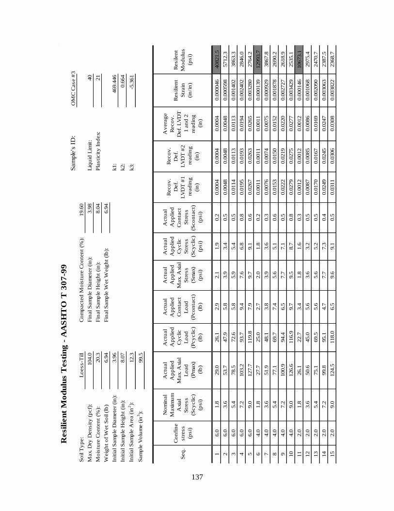
137

Resil

ien

t M

od

ulu

s T

esti

ng

- A

AS

HT

O T

30

7-9

9S

am

ple

's I

D:

OM

C C

ase #

3

So

il T

yp

e:

Lo

ess-T

ill

Co

mp

acte

d M

ois

ture

Co

nte

nt

(%):

19.6

0

Max.

Dry

Den

sit

y (

pcf)

:104.0

Fin

al S

am

ple

Dia

mete

r (i

n):

3.9

8L

iqu

id L

imit

:40

Mo

istu

re C

on

ten

t (%

):20.3

Fin

al S

am

ple

Heig

ht

(in

):8.0

4P

lasti

cit

y I

nd

ex:

21

Weig

ht

of

Wet

So

il (

lb)

6.9

4F

inal S

am

ple

Wet

Weig

ht

(lb

):6.9

4

Init

ial S

am

ple

Dia

mete

r (i

n):

3.9

6k1:

469.4

46

Init

ial S

am

ple

Heig

ht

(in

):8.0

7k2:

0.6

64

Init

ial S

am

ple

Are

a (

in2):

12.3

k3:

-5.3

61

Sam

ple

Vo

lum

e (

in3):

99.5

Seq

.

Co

nfi

ne

str

ess

(psi)

No

min

al

Maxi

mu

m

Axi

al

Str

ess

(Scy

clic)

(psi)

Actu

al

Ap

plied

Max.

Axi

al

Lo

ad

(P

max)

(lb

)

Actu

al

Ap

plied

Cy

clic

Lo

ad

(Pcy

clic)

(lb

)

Actu

al

Ap

plied

Co

nta

ct

Lo

ad

(Pco

nta

ct)

(lb

)

Actu

al

Ap

plied

Max.

Axi

al

Str

ess

(Sm

ax)

(psi)

Actu

al

Ap

plied

Cy

clic

Str

ess

(Scy

clic)

(psi)

Actu

al

Ap

plied

Co

nta

ct

Str

ess

(Sco

nta

ct)

(p

si)

Reco

v.

Def.

LV

DT

#1

read

ing

(in

)

Reco

v.

Def.

LV

DT

#2

read

ing

(in

)

Av

era

ge

Reco

v.

Def.

LV

DT

1 a

nd

2

read

ing

(in

)

Resilie

nt

Str

ain

(in

/in

)

Resilen

t

Mo

du

lus

(psi)

16.0

1.8

29.0

26.1

2.9

2.1

1.9

0.2

0.0

004

0.0

004

0.0

004

0.0

00046

40821.5

26.0

3.6

53.7

47.9

5.8

3.9

3.4

0.5

0.0

048

0.0

048

0.0

048

0.0

00598

5712.3

36.0

5.4

78.5

72.6

5.8

5.9

5.4

0.5

0.0

114

0.0

113

0.0

113

0.0

01402

3863.3

46.0

7.2

103.2

93.7

9.4

7.6

6.8

0.8

0.0

195

0.0

193

0.0

194

0.0

02402

2846.0

56.0

9.0

127.7

119.8

7.9

9.7

9.1

0.6

0.0

267

0.0

263

0.0

265

0.0

03280

2764.2

64.0

1.8

27.7

25.0

2.7

2.0

1.8

0.2

0.0

011

0.0

011

0.0

011

0.0

00139

12993.7

74.0

3.6

51.9

48.1

3.8

3.9

3.6

0.3

0.0

076

0.0

074

0.0

075

0.0

00929

3867.8

84.0

5.4

77.1

69.7

7.4

5.6

5.1

0.6

0.0

153

0.0

150

0.0

152

0.0

01878

2690.2

94.0

7.2

100.9

94.4

6.5

7.7

7.1

0.5

0.0

222

0.0

219

0.0

220

0.0

02727

2618.9

10

4.0

9.0

126.6

116.9

9.7

9.5

8.7

0.8

0.0

279

0.0

275

0.0

277

0.0

03429

2535.1

11

2.0

1.8

26.1

22.7

3.4

1.8

1.6

0.3

0.0

012

0.0

012

0.0

012

0.0

00146

10673.1

12

2.0

3.6

50.6

45.0

5.6

3.6

3.2

0.5

0.0

087

0.0

085

0.0

086

0.0

01068

2975.4

13

2.0

5.4

75.1

69.5

5.6

5.6

5.2

0.5

0.0

170

0.0

167

0.0

169

0.0

02090

2470.7

14

2.0

7.2

99.8

95.1

4.7

7.7

7.3

0.4

0.0

249

0.0

245

0.0

247

0.0

03063

2387.5

15

2.0

9.0

124.5

118.0

6.5

9.6

9.1

0.5

0.0

311

0.0

306

0.0

308

0.0

03822

2368.7

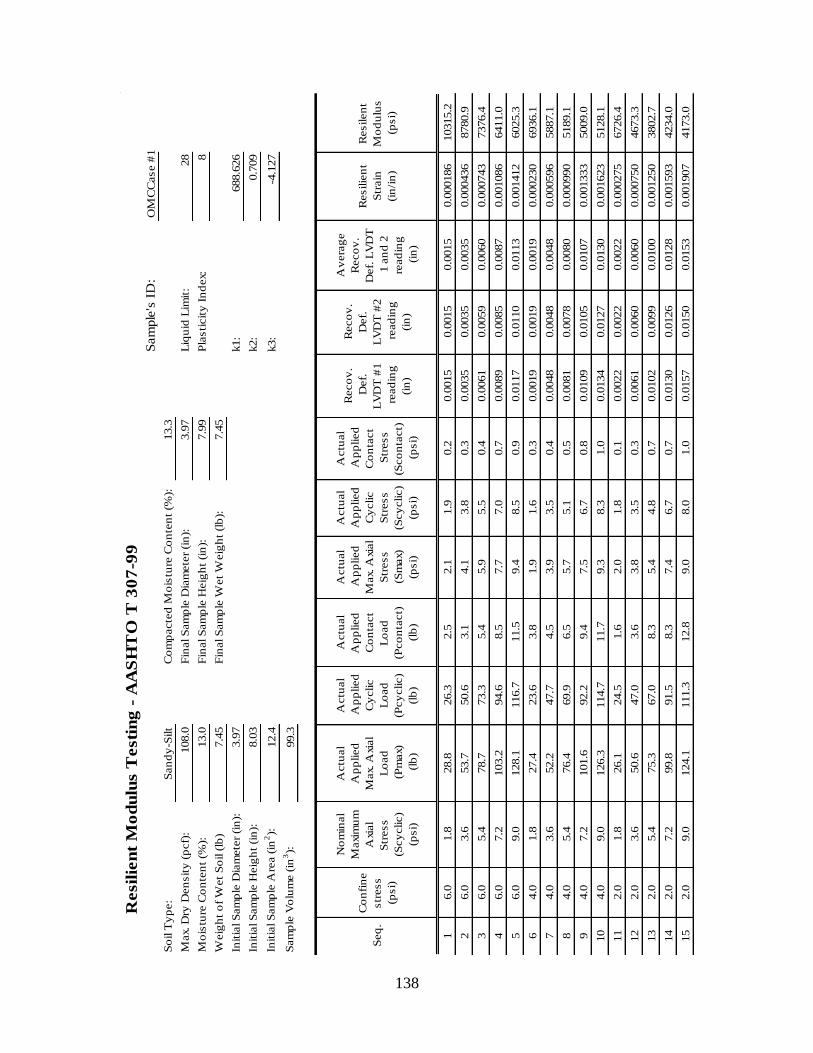
138

Resil

ien

t M

od

ulu

s T

esti

ng

- A

AS

HT

O T

30

7-9

9S

am

ple

's I

D:

OM

CC

ase #

1

So

il T

yp

e:

San

dy

-Silt

Co

mp

acte

d M

ois

ture

Co

nte

nt

(%):

13.3

Max.

Dry

Den

sit

y (

pcf)

:108.0

Fin

al S

am

ple

Dia

mete

r (i

n):

3.9

7L

iqu

id L

imit

:28

Mo

istu

re C

on

ten

t (%

):13.0

Fin

al S

am

ple

Heig

ht

(in

):7.9

9P

lasti

cit

y I

nd

ex:

8

Weig

ht

of

Wet

So

il (

lb)

7.4

5F

inal S

am

ple

Wet

Weig

ht

(lb

):7.4

5

Init

ial S

am

ple

Dia

mete

r (i

n):

3.9

7k1:

688.6

26

Init

ial S

am

ple

Heig

ht

(in

):8.0

3k2:

0.7

09

Init

ial S

am

ple

Are

a (

in2):

12.4

k3:

-4.1

27

Sam

ple

Vo

lum

e (

in3):

99.3

Seq

.

Co

nfi

ne

str

ess

(psi)

No

min

al

Maxi

mu

m

Axi

al

Str

ess

(Scy

clic)

(psi)

Actu

al

Ap

plied

Max.

Axi

al

Lo

ad

(P

max)

(lb

)

Actu

al

Ap

plied

Cy

clic

Lo

ad

(Pcy

clic)

(lb

)

Actu

al

Ap

plied

Co

nta

ct

Lo

ad

(Pco

nta

ct)

(lb

)

Actu

al

Ap

plied

Max.

Axi

al

Str

ess

(Sm

ax)

(psi)

Actu

al

Ap

plied

Cy

clic

Str

ess

(Scy

clic)

(psi)

Actu

al

Ap

plied

Co

nta

ct

Str

ess

(Sco

nta

ct)

(p

si)

Reco

v.

Def.

LV

DT

#1

read

ing

(in

)

Reco

v.

Def.

LV

DT

#2

read

ing

(in

)

Av

era

ge

Reco

v.

Def.

LV

DT

1 a

nd

2

read

ing

(in

)

Resilie

nt

Str

ain

(in

/in

)

Resilen

t

Mo

du

lus

(psi)

16.0

1.8

28.8

26.3

2.5

2.1

1.9

0.2

0.0

015

0.0

015

0.0

015

0.0

00186

10315.2

26.0

3.6

53.7

50.6

3.1

4.1

3.8

0.3

0.0

035

0.0

035

0.0

035

0.0

00436

8780.9

36.0

5.4

78.7

73.3

5.4

5.9

5.5

0.4

0.0

061

0.0

059

0.0

060

0.0

00743

7376.4

46.0

7.2

103.2

94.6

8.5

7.7

7.0

0.7

0.0

089

0.0

085

0.0

087

0.0

01086

6411.0

56.0

9.0

128.1

116.7

11.5

9.4

8.5

0.9

0.0

117

0.0

110

0.0

113

0.0

01412

6025.3

64.0

1.8

27.4

23.6

3.8

1.9

1.6

0.3

0.0

019

0.0

019

0.0

019

0.0

00230

6936.1

74.0

3.6

52.2

47.7

4.5

3.9

3.5

0.4

0.0

048

0.0

048

0.0

048

0.0

00596

5887.1

84.0

5.4

76.4

69.9

6.5

5.7

5.1

0.5

0.0

081

0.0

078

0.0

080

0.0

00990

5189.1

94.0

7.2

101.6

92.2

9.4

7.5

6.7

0.8

0.0

109

0.0

105

0.0

107

0.0

01333

5009.0

10

4.0

9.0

126.3

114.7

11.7

9.3

8.3

1.0

0.0

134

0.0

127

0.0

130

0.0

01623

5128.1

11

2.0

1.8

26.1

24.5

1.6

2.0

1.8

0.1

0.0

022

0.0

022

0.0

022

0.0

00275

6726.4

12

2.0

3.6

50.6

47.0

3.6

3.8

3.5

0.3

0.0

061

0.0

060

0.0

060

0.0

00750

4673.3

13

2.0

5.4

75.3

67.0

8.3

5.4

4.8

0.7

0.0

102

0.0

099

0.0

100

0.0

01250

3802.7

14

2.0

7.2

99.8

91.5

8.3

7.4

6.7

0.7

0.0

130

0.0

126

0.0

128

0.0

01593

4234.0

15

2.0

9.0

124.1

111.3

12.8

9.0

8.0

1.0

0.0

157

0.0

150

0.0

153

0.0

01907

4173.0

139

Resil

ien

t M

od

ulu

s T

esti

ng

- A

AS

HT

O T

30

7-9

9S

am

ple

's I

D:

OM

CC

ase #

2

So

il T

yp

e:

San

dy

-Silt

Co

mp

acte

d M

ois

ture

Co

nte

nt

(%):

13.1

Max.

Dry

Den

sit

y (

pcf)

:108.0

Fin

al S

am

ple

Dia

mete

r (i

n):

3.9

6L

iqu

id L

imit

:28

Mo

istu

re C

on

ten

t (%

):13.0

Fin

al S

am

ple

Heig

ht

(in

):7.9

8P

lasti

cit

y I

nd

ex:

8

Weig

ht

of

Wet

So

il (

lb)

7.5

3F

inal S

am

ple

Wet

Weig

ht

(lb

):7.5

3

Init

ial S

am

ple

Dia

mete

r (i

n):

3.9

6k1:

726.8

77

Init

ial S

am

ple

Heig

ht

(in

):8.0

5k2:

0.3

50

Init

ial S

am

ple

Are

a (

in2):

12.3

k3:

-1.9

96

Sam

ple

Vo

lum

e (

in3):

99.0

Seq

.

Co

nfi

ne

str

ess

(psi)

No

min

al

Maxi

mu

m

Axi

al

Str

ess

(Scy

clic)

(psi)

Actu

al

Ap

plied

Max.

Axi

al

Lo

ad

(P

max)

(lb

)

Actu

al

Ap

plied

Cy

clic

Lo

ad

(Pcy

clic)

(lb

)

Actu

al

Ap

plied

Co

nta

ct

Lo

ad

(Pco

nta

ct)

(lb

)

Actu

al

Ap

plied

Max.

Axi

al

Str

ess

(Sm

ax)

(psi)

Actu

al

Ap

plied

Cy

clic

Str

ess

(Scy

clic)

(psi)

Actu

al

Ap

plied

Co

nta

ct

Str

ess

(Sco

nta

ct)

(p

si)

Reco

v.

Def.

LV

DT

#1

read

ing

(in

)

Reco

v.

Def.

LV

DT

#2

read

ing

(in

)

Av

era

ge

Reco

v.

Def.

LV

DT

1 a

nd

2

read

ing

(in

)

Resilie

nt

Str

ain

(in

/in

)

Resilen

t

Mo

du

lus

(psi)

16.0

1.8

29.0

26.5

2.5

2.2

2.0

0.2

0.0

004

0.0

003

0.0

003

0.0

00039

50114.6

26.0

3.6

53.5

48.6

4.9

3.9

3.5

0.4

0.0

022

0.0

020

0.0

021

0.0

00262

13547.8

36.0

5.4

78.2

71.0

7.2

5.8

5.2

0.6

0.0

044

0.0

042

0.0

043

0.0

00538

9631.5

46.0

7.2

103.0

93.1

9.9

7.6

6.8

0.8

0.0

064

0.0

061

0.0

062

0.0

00775

8744.8

56.0

9.0

127.2

114.9

12.4

9.3

8.3

1.0

0.0

085

0.0

082

0.0

083

0.0

01034

8058.7

64.0

1.8

27.4

25.0

2.5

2.0

1.8

0.2

0.0

004

0.0

002

0.0

003

0.0

00037

49872.7

74.0

3.6

51.9

47.0

4.9

3.8

3.4

0.4

0.0

022

0.0

020

0.0

021

0.0

00267

12840.4

84.0

5.4

76.7

69.2

7.4

5.6

5.0

0.6

0.0

052

0.0

049

0.0

050

0.0

00626

8057.8

94.0

7.2

101.6

91.7

9.9

7.4

6.6

0.8

0.0

073

0.0

070

0.0

072

0.0

00892

7448.7

10

4.0

9.0

125.9

113.5

12.4

9.2

8.2

1.0

0.0

091

0.0

088

0.0

090

0.0

01112

7387.4

11

2.0

1.8

26.1

23.6

2.5

1.9

1.7

0.2

0.0

004

0.0

003

0.0

003

0.0

00042

41203.3

12

2.0

3.6

50.4

45.4

4.9

3.7

3.3

0.4

0.0

026

0.0

024

0.0

025

0.0

00313

10509.0

13

2.0

5.4

75.3

67.9

7.4

5.5

4.9

0.6

0.0

057

0.0

055

0.0

056

0.0

00699

7046.9

14

2.0

7.2

99.8

89.9

9.9

7.3

6.5

0.8

0.0

074

0.0

071

0.0

073

0.0

00902

7222.9

15

2.0

9.0

124.3

112.0

12.4

9.1

8.1

1.0

0.0

095

0.0

093

0.0

094

0.0

01169

6936.8

140

Resil

ien

t M

od

ulu

s T

esti

ng

- A

AS

HT

O T

30

7-9

9S

am

ple

's I

D:

OM

CC

ase #

3

So

il T

yp

e:

San

dy

-Silt

Co

mp

acte

d M

ois

ture

Co

nte

nt

(%):

13.2

Max.

Dry

Den

sit

y (

pcf)

:108.0

Fin

al S

am

ple

Dia

mete

r (i

n):

3.9

8L

iqu

id L

imit

:28

Mo

istu

re C

on

ten

t (%

):13.0

Fin

al S

am

ple

Heig

ht

(in

):8.0

3P

lasti

cit

y I

nd

ex:

8

Weig

ht

of

Wet

So

il (

lb)

7.4

4F

inal S

am

ple

Wet

Weig

ht

(lb

):7.4

4

Init

ial S

am

ple

Dia

mete

r (i

n):

3.9

8k1:

860.5

32

Init

ial S

am

ple

Heig

ht

(in

):8.0

4k2:

0.5

62

Init

ial S

am

ple

Are

a (

in2):

12.4

k3:

-1.7

03

Sam

ple

Vo

lum

e (

in3):

99.9

Seq

.

Co

nfi

ne

str

ess

(psi)

No

min

al

Maxi

mu

m

Axi

al

Str

ess

(Scy

clic)

(psi)

Actu

al

Ap

plied

Max.

Axi

al

Lo

ad

(P

max)

(lb

)

Actu

al

Ap

plied

Cy

clic

Lo

ad

(Pcy

clic)

(lb

)

Actu

al

Ap

plied

Co

nta

ct

Lo

ad

(Pco

nta

ct)

(lb

)

Actu

al

Ap

plied

Max.

Axi

al

Str

ess

(Sm

ax)

(psi)

Actu

al

Ap

plied

Cy

clic

Str

ess

(Scy

clic)

(psi)

Actu

al

Ap

plied

Co

nta

ct

Str

ess

(Sco

nta

ct)

(p

si)

Reco

v.

Def.

LV

DT

#1

read

ing

(in

)

Reco

v.

Def.

LV

DT

#2

read

ing

(in

)

Av

era

ge

Reco

v.

Def.

LV

DT

1 a

nd

2

read

ing

(in

)

Resilie

nt

Str

ain

(in

/in

)

Resilen

t

Mo

du

lus

(psi)

16.0

1.8

29.2

27.2

2.0

2.2

2.0

0.2

0.0

079

0.0

080

0.0

080

0.0

00991

2043.9

26.0

3.6

54.0

49.0

4.9

4.0

3.6

0.4

0.0

022

0.0

021

0.0

021

0.0

00267

13310.7

36.0

5.4

78.9

71.5

7.4

5.8

5.2

0.6

0.0

033

0.0

032

0.0

032

0.0

00404

12787.0

46.0

7.2

103.6

93.7

9.9

7.6

6.8

0.8

0.0

045

0.0

045

0.0

045

0.0

00560

12060.3

56.0

9.0

128.4

116.0

12.4

9.3

8.3

1.0

0.0

058

0.0

057

0.0

058

0.0

00717

11614.0

64.0

1.8

27.7

25.6

2.0

2.1

1.9

0.2

0.0

079

0.0

080

0.0

080

0.0

00989

1929.5

74.0

3.6

52.4

47.4

4.9

3.8

3.4

0.4

0.0

026

0.0

026

0.0

026

0.0

00321

10672.7

84.0

5.4

77.3

69.9

7.4

5.6

5.0

0.6

0.0

039

0.0

039

0.0

039

0.0

00485

10410.7

94.0

7.2

102.5

92.6

9.9

7.4

6.7

0.8

0.0

053

0.0

052

0.0

053

0.0

00653

10182.9

10

4.0

9.0

126.6

114.2

12.4

9.2

8.2

1.0

0.0

065

0.0

065

0.0

065

0.0

00803

10214.8

11

2.0

1.8

26.3

24.3

2.0

2.0

1.8

0.2

0.0

076

0.0

077

0.0

077

0.0

00954

1892.3

12

2.0

3.6

51.0

45.9

5.2

3.7

3.3

0.4

0.0

032

0.0

032

0.0

032

0.0

00399

8232.0

13

2.0

5.4

76.0

68.6

7.4

5.5

4.9

0.6

0.0

048

0.0

047

0.0

047

0.0

00590

8342.7

14

2.0

7.2

100.7

90.8

9.9

7.3

6.5

0.8

0.0

062

0.0

062

0.0

062

0.0

00771

8442.7

15

2.0

9.0

125.4

113.1

12.4

9.1

8.1

1.0

0.0

075

0.0

075

0.0

075

0.0

00935

8668.8

141

Resil

ien

t M

od

ulu

s T

esti

ng

- A

AS

HT

O T

30

7-9

9S

am

ple

's I

D:

OM

CC

ase #

4

So

il T

yp

e:

San

dy

-Silt

Co

mp

acte

d M

ois

ture

Co

nte

nt

(%):

13.3

Max. D

ry D

en

sit

y (

pcf)

:108.0

Fin

al S

am

ple

Dia

mete

r (i

n):

3.9

9L

iqu

id L

imit

:28

Mo

istu

re C

on

ten

t (%

):13.0

Fin

al S

am

ple

Heig

ht

(in

):8.0

6P

lasti

cit

y I

nd

ex:

8

Weig

ht

of

Wet

So

il (

lb)

7.4

4F

inal S

am

ple

Wet

Weig

ht

(lb

):7.3

1

Init

ial S

am

ple

Dia

mete

r (i

n):

3.9

8k1:

846.2

94

Init

ial S

am

ple

Heig

ht

(in

):8.0

6k2:

0.3

51

Init

ial S

am

ple

Are

a (

in2):

12.4

k3:

-1.5

80

Sam

ple

Vo

lum

e (

in3):

100.1

Seq

.

Co

nfi

ne

str

ess

(psi)

No

min

al

Maxim

um

Axia

l

Str

ess

(Scy

clic)

(psi)

Actu

al

Ap

plied

Max. A

xia

l

Lo

ad

(P

max)

(lb

)

Actu

al

Ap

plied

Cy

clic

Lo

ad

(Pcy

clic)

(lb

)

Actu

al

Ap

plied

Co

nta

ct

Lo

ad

(Pco

nta

ct)

(lb

)

Actu

al

Ap

plied

Max. A

xia

l

Str

ess

(Sm

ax)

(psi)

Actu

al

Ap

plied

Cy

clic

Str

ess

(Scy

clic)

(psi)

Actu

al

Ap

plied

Co

nta

ct

Str

ess

(Sco

nta

ct)

(p

si)

Reco

v.

Def.

LV

DT

#1

read

ing

(in

)

Reco

v.

Def.

LV

DT

#2

read

ing

(in

)

Av

era

ge

Reco

v.

Def.

LV

DT

1 a

nd

2

read

ing

(in

)

Resilie

nt

Str

ain

(in

/in

)

Resilen

t

Mo

du

lus

(psi)

16.0

1.8

29.2

26.8

2.5

2.2

2.0

0.2

0.0

012

0.0

012

0.0

012

0.0

00149

13094.0

26.0

3.6

54.0

49.0

4.9

3.9

3.5

0.4

0.0

025

0.0

024

0.0

025

0.0

00305

11611.1

36.0

5.4

78.9

71.5

7.4

5.8

5.2

0.6

0.0

039

0.0

037

0.0

038

0.0

00474

10897.3

46.0

7.2

103.6

93.7

9.9

7.6

6.8

0.8

0.0

052

0.0

050

0.0

051

0.0

00632

10689.0

56.0

9.0

128.4

116.0

12.4

9.3

8.3

1.0

0.0

062

0.0

058

0.0

060

0.0

00747

11156.4

64.0

1.8

27.7

25.2

2.5

2.0

1.8

0.2

0.0

012

0.0

012

0.0

012

0.0

00149

12256.4

74.0

3.6

52.4

47.4

4.9

3.8

3.4

0.4

0.0

028

0.0

026

0.0

027

0.0

00339

10073.6

84.0

5.4

77.6

70.1

7.4

5.6

5.1

0.6

0.0

044

0.0

041

0.0

043

0.0

00530

9537.8

94.0

7.2

102.3

92.4

9.9

7.4

6.6

0.8

0.0

057

0.0

053

0.0

055

0.0

00681

9749.8

10

4.0

9.0

126.8

114.4

12.4

9.2

8.2

1.0

0.0

066

0.0

062

0.0

064

0.0

00793

10365.4

11

2.0

1.8

26.3

23.8

2.5

1.9

1.7

0.2

0.0

015

0.0

014

0.0

014

0.0

00176

9718.1

12

2.0

3.6

51.0

46.1

4.9

3.7

3.3

0.4

0.0

033

0.0

031

0.0

032

0.0

00396

8338.7

13

2.0

5.4

76.0

68.6

7.4

5.5

4.9

0.6

0.0

050

0.0

047

0.0

048

0.0

00598

8226.8

14

2.0

7.2

100.7

90.8

9.9

7.3

6.5

0.8

0.0

062

0.0

059

0.0

060

0.0

00750

8694.0

15

2.0

9.0

125.2

112.9

12.4

9.1

8.1

1.0

0.0

073

0.0

069

0.0

071

0.0

00881

9187.4

layer moduli of nebraska pavements for the new...

Documents