lawrence berkeley laboratory - steve omohundro · 2009-03-06 · geometric hamiltonian structures...
TRANSCRIPT

LBL-18302
Lawrence Berkeley Laboratory UNIVERSITY OF CALIFORNIA
Accelerator amp Fusion Research Division
P resented at the NRL-NSWC Workshop o n Local amp Global Methods of Dynamics Naval Surface Weapons Center Silver Spri ng Maryland July 23-26 1984
GEOMETRIC HAMILTONIAN STRUCTURES AND PERTURBATION THEORY
S Omohundro
August 19 84
Prepared for the US Department of Energy under Contract DE-AC03-76SF00098
LBL-18302
Geometric Hamiltonian Structures and Perturbation Theory
Stephen Omohundro Lawrence Berkeley Laboratory and Physics Department
University of California 8erkeley CA 94120
August 1984
This work was supported by the Office of Basic Energy Sciences of the US Department of Energy under Contract No DE-AC03-16SF00098
Geometric Hamiltonian Structures and Perturbation Theory t
by Stephen Omohundro
Lawrence Berkeley Laboratory and Physics Department
University of California
Berkeley CA 94720
I Introduction
In this lecture we discuss the ideas in reference [25] intuitively and heuristically That
paper assumes a background in geometric mechanics and has detailed proofs Here we will give
the flavor of the structures and develop the needed background material We will state the
results and indicate why they are true without detailed proof We begin with some introductory
remarks discuss a geometric picture for non-singular perturbation theory introduce the needed
Hamiltonian mechanics including the crucial process of reduction in the presence of symmetry
describe the Hamiltonian structure of non-singular perturbation theory and close with some
discussion of these ideas in connection with the method of averaging
Dr Deprits lecture has described the intimate historical connections between perturbashy
tion theory and Hamiltonian mechanics It is of interest to list the seminal ideas that form the
background of the present work In 1808 Lagrange introduced the description of the dynamics
of celestial bodies in terms of what we today call Hamiltons equations12 His motivation was
the reduction of the enormous labor involved in a straightforward perturbation analysis which
required tedious computations to be performed on each component of the dynamical vector field
to manipulations of a single function themiddot Hamiltonian The description in terms of Lagrange
brackets led to several other benefits Lagrange showed that the value of the Hamiltonian and
the structure of the brackets were both invariant under the dynamics leading to a useful check
of the complex calculations (which at that time were done by hand) In addition he was able
to show that the invariance of the Hamiltonian could be used to prove stability of certain equishy
libria As the century progressed Hamiltonian mechanics was refined and the connections with
variational principles and optics were made By the tum of the century Poincare3 had developed
very powerful Hamiltonian perturbation methods utilizing generating functions introduced the
notion of asymptotic expansion and begun the geometric and topological approach to dynamshy
ics In 1918 Emmy Noether4 made the ~onnection between symmetries and conserved quantishy
ties The development of quantum mechanics rested heavily on the Hamiltonian frameworks by
analogy with optics and served to put it firmly at the center of the modem formulation of funshy
damental physics6 bull During the 1960s the coordinate free description of Hamiltonian structures
in terms of symplectic geometry was developed7bull8 bull About this time the Hamiltonian method of
Lie transforms greatly simplified Hamiltonian perturbation theory9 The 1970s saw enormous
t This work was supported by the Office of Basic Energy Sciences of the US Department of
Energy under Contract No DE-AC03-76SF00098
- 1 shy
developments in the geometric approach to mechanics and largely as a result of these an ever
wider range of physical systems have been described in Hamiltonian terms Some examples are
quantum mechanicsl0 fluid mechanics11 1213 M~ells equations1516 the MaxWell-Vlasov and Poisson-Vlasov1415 equations of plasma physics elasticity theory1718 general relativity18
magnetohydrodynamics11 17 multi-fluid plasmas 1719 chromohydrodynamics20 superfluids and
superconductors21 the Korteweg de Vries equation22 etc These developments have shed light
on the underlying synunetry structure of these theories have yielded improved stability results
based on Arnolds stability method23 and have given insight into the reasons for the integrability
of certain systems24
For the most parthowever these structures describe fundamental underlying models in the
various fields In actual applications we almost always make numerous approximations which may
or may not respect the underlying Hamiltonian structure It is folklore within the particle physics
community and elsewhere that perturbation methods which respect the underlying symmetries
and conservation laws yield much better approximations to the actual system than those which
do not It is of interest then to try to do perturbation theory within the Hamiltonian framework
and to obtain structures relevant to the approximate system One may thus hope to understand
the relation between the structures of systems which are limiting cases of known systems (eg
does the KdV Poisson bracket arise naturally from that of the Boussinesq equations) 31 The
history of Hamiltonian mechanics is inextricably tied to perturbation methods For the most
part though the Hamiltonian structure was used to simplify the perturbation method and the
geometric structure of the perturbation method itself was not explored We have found in several
examples that taking this structure into account leads to simplifications (as in the problem of
guiding center motion discussed later in this paper) and to deeper insight into the approximate
system (as in modulational equations for waves in the eikonal limit )26
We have therefore been engaged in a program of investigating the Hamiltonian structure
of the various perturbation theories used in practice In this paper we describe the geometry
of a Hamiltonian structure for non-singular perturbation theory applied to Hamiltonian systems
on symplectic manifolds and the connection with singular perturbation techniques based on the
method of averaging
II Geometric Perturbation TheorY
The modern setting for describing an evolving system is a dynamical system The state of the
system is represented by a point in a manifold M A manifold is a space which locally looks like
Euclidean space and in which there is a notion of derivative Globally a manifold may be connected
together in a funny way as in a sphere or a torus If you know where you are the dynamics tells
you where youre going Thus dynamics is represented by a vector field on the manifold of states
A dynamical system is a manifold with a vector field defined on it In coordinates the dynamics
gives a set of first order ODEs one for each coordinate Typical dynamical systems with
state spaces of three dimensions or greater have chaotic dynamics with extremely complicated
- 2 shy
trajectories for which one can prove there is no closed form exact description If the dynamics
simplifies then there is usually some physically relevant special feature such as a symmetry which
causes the simplification
In important physical applications we often find otiselves close to a system which simplifies
and we are interested in the effect of our deviation from it We express this deviation in terms of
the small parameter e If we are given dynamics in the form
213 X =Xo + eXl + 2X2 + (I)
in terms of the vector fields Xi with initial conditions described by x13 t = 0) = ye) we may
attempt to express the solution in an asymptotic series in e
(2)
Choosing coordinates XCI (I 5 a 5 N) in a local patch and plugging thiS assumed asymptotic
form into the equation of motion gives
2 2 bull CI bull CI e bull CI XCI ( e )Xo + eXl + 2 x2 + = 0 Xo + eXl + 2 X2 + +
2e (3)+ eXf(xo + eXl + 2 X2 + )+
e2 e2
+ X~(xo + eXl + X2 + ) + 2 2
Since asymptotic expansions are unique we may equate coefficients of equal powers of e to get
equations for xo xl
(4)
H y(e) = Yo + eYl + E Y2 + is an asymptotic expansion for the initial condition y(e) then the
initial conditions for these equations are xo(t = 0) = YOXl (t = 0) = Yllmiddotmiddotmiddotmiddot
These equations immediately raise a number of questions They are defined in terms of
physically irrelevant coordinates is the perturbation structure independent of these coordinates
If the original equations are Hamiltonian are these equations In Jth order perturbation theory
how are we to interpret this evolution of many variables xo xl X The goal of this work is
to answer these questions
- 3 shy
Let us turn to the geometric interpretation of these equations It is easiest to understand
the first order perturbation equations
xg = xg(Xo)
0 ~ BXg ( ) b XO( )Xl =~ Bxb Xo Xl + 1 Xo (5)
b=l
XO(t = 0) = Yo Xl(t = 0) = Yl
We would like to determine the geometric nature of the quantities Xo and Xl To understand what
we mean by this let us recall the relationship between geometric quantities and coordinates A
function on a manifold is an intrinsically defined thing it assigns a real number to each point of the
manifold A coordinate system on a region of an N dimensional manifold is a collection of N real
valued functions xl xN defined on that region whose differentials are linearly independent
at each point In these coordinates the gradient of a function is a collection of N numbers the
derivatives with respect to each of the xo Geometrically however it is wrong to think of these
as just real numbers because they change if we change our coordinate system For example if
we choose coordinates whose values at each point of the region are twice those of xl xN then
the components of the gradient of a function are halved We introduce a geometric object whose
relationship to the manifold at a given point is like that of the gradient of a function and we call
it a covector or one-form The collection of all covectors at a point is defined to be the cotangent
space at that point and the collection of all cotangent spaces taken together form the cotangent
bundle Similarly the components of a vector at a point double with the coordinates All vectors
at a point taken together form the tangent space at that point and all tangent spaces taken
together form the tangent bundle T M of M Vectors and covectors are thus different objects
when we consider more than one coordinate system even though they both have N components
in any given system Our interest here will be to find out whether the quantities xg x for
1 $ a $ N have any geometric structure that is independent of a given coordinate system
Intuitively the first order quantity Xl represents a small deviation from the unperturbed
quantity Xo Because Xo can vary over the whole manifold M we expect it to represent a point
in the manifold As f gets smaller Xo + fXI approaches the point Xo and Xl measures the first
order rate of approach to Xo Two different paths in the manifold approaching the point Xo as
( approaches zero have the same Xl if and only if they are tangent at Xo This however is the
defining criterion for a vector at the point Xo We thus expect Xl to lie in the tangent space to
Mover the point Xo- The XOXl dynamics then takes place on the tangent bundle TM We will
describe this dynamics on TM intrinsically in terms of vector fields derived from X(f) on M
The solution of a system of ODEs tells us the state at each time t of a system which
began with each initial condition Geometrically this is a mapping of M to itself for each t If
the solution doesnt run off of the manifold then the uniqueness and smoothness of solutions
with given intial conditions tells us that this map is a diffeomorpbism (ie a smooth 1-1 onto
map with smooth inverse) This one-parameter family of diffeomorphisms labelled by t is called
the flow of the dynamical vector field As ( varies the corresponding Hows of X(f) will vary
- 4 shy
Perturbation theory describes that variation Any time we have a mapping f from one manifold
to another we may define its diJIerential T f This is a map that takes the tangent bundle of the
first manifold to the tangent bundle of the second It describes how infinitesimal perturbations
at a point are sent to infinitesimal perturbations at the image point In coordinates it acts on
the tangent space at a point via the Jacobian matrix of f at that point
Through abuse of notation let us denote the How of the unperturbed vector field Xo by
xo(t) xo(t Yo) is the point to which Yo has Howed in time t under Xo A small perturbation in
M from a given orbit will evolve under Xo according to the derivative of this How Txo(t) This
is a How on the manifold T M and the vector field of which it is the How may be written
Xo- == ddl Txo(t) (6) t t=O
Xo is a vector field on T M defined without recourse to coordinates that represents the effect of
the unperturbed How on perturbed orbits In coordinates Xo has components
(7)
This dynamics is exactly that part of the perturbation dynamics (5) which depends on Xo The
part which depends on Xl may also be defined intrinsically If we define
(8)
then the entire first order perturbation dynamics on T M is given by
(9)
ITI The Geometry of Jth Order Perturbation Theory
We have succeeded in finding a geometric coordinate-free interpretation for first order pershy
turbation theory We now would like to extend this to higher orders The geometric object that
arises is called a jet To understand the setting we discuss a number of relevant spaces
How are we to think of the exact equation for the evolution of an t dependent point x( t)
under t dependent evolution equations x(t) = X(tx) with t dependent initial conditions Y(t)
It is useful to think of thef dependent point x(t) as a curve in the space I x M where I is the
interval (say [01]) in which t takes its values If we thinkof x(t) as a map from I to 11 then the
curve is the graph of this map The dynamical vector field X(t) naturally lives on I X lw and its
I component is zero everywhere The How of Xt) on I x M takes paths to paths by letting each
point of a path move with the How Our initial conditions are represented by paths (if they are
- 5 shy
independent of euro then they are straight lines) The true dynamics takes paths to paths Even if
the intial conditions are euro independent the dynamics bends the path over Thus we really should
think of our dynamics as living on the infinite dimensional path space
P1M = space of all paths p I - I x M of the form p euro 1--+ (fX(f)) (10)
where as before 1= [OIJ
This projects naturally onto
PoM = equivalence classes in P1M where PI rv P2 iff PI (0) =P2(0) (11)
PoM is naturally isomorphic to M and represents the domain of the unperturbed dynamics The
equivalence classes forget all perturbation information and only remember behavior at f = O We
are interested in spaces through which this projection of real to unperturbed dynamics factors
Perturbation theory tries to study behavior infinitesimally close to f = 0 without actually getting
there For each 0 ~ a ~ 1 we may define
These allow us to consider more and more restricted domains of f but there is always a continuum
of fS to traverse before reaching f =O For each 1 al a2 0 we have the natural maps
(13)
We are interested in structure between even the smallest PaM with a f 0 and PoM We may
introduce germs of paths
GM =eqUivalence classes in PIM where PI rv P2 iff (14)
3a gt 0 such that PI(f) = P2(f) V0 ~ f ~ a
and for any a gt 0 we have PaM - GM - POi The germs capture behavior closer to f = 0
than any given f but still contain much more information than perturbation theory gives us
(germs depend on features of function in a little neighborhood that are not captured in a Taylor
series)
Finally we may introduce spaces of jets of paths at f - 0 with integer 1 ~ J ~ 00
J M = eqUiValence classes in P1M where PI rv P2 iff
V Coo functions f on I x M we have (15)
for 0 ~i leo f(pdf)) = IE=o (p2(euro)) i $ J - 6 shy
Thus the space of J-jets gives the first J terms in a Taylor expansion of the cUJVe around l = 0
in any coordinate system Clearly
GM - ooM -1M - JM -PoM for Igt J
Thus the jets focus on information closer to f =0 than even the germs
If x for 1 ~ a ~ N are coordinates on M Rl PoM Rl OM then we may introduce coordinates
xo xr xj for 0 ~ J ~ 00 on J M to represent the equivalence class of the curve
in I x M (near E = 0 this wont leave the chart on which the x are defined)
The claim here is that J 41 represents geometrically the perturbation quantities xo x J bull
It may seem strange to go through the infinite dimensional space PI M to get to it but we
shall see (especially when looking at the Hamiltonian structure) that it organizes and simplifies
the structures of interest It is a completely intrinsic and natural (category theorists would say
functorial) operation to go from the original dynamical manifold M to the path space PIM to the
jet space J kf We shall now show that the dyanamics on M also induces natural dynamics on PIM
and then projects from there down to J M where it is the perturbation dynamics we are interested
in Later we will show that a Hamiltonian structure on M leads to Hamiltonian structures on
PIM and JM The dynamics x= X(fx) takes elements of PIM to other elements of PIM and
in fact takes equivalence classes to equivalence classes for each of PaM GM ooM J M and M
This is what allows us to obtain an induced dynamics on each of these spaces To determine this
dynamics explicitly we must understand what a tangent vector on each space is
Intuitively a vector represents a little perturbation to a point We define it precisely as an
equivalence class of tangent curves where the curve represents the direction of perturbation and
the equivalence class ensures that only the first order motion is reflected in the tangent vector
A point in the path space PI M is a path in I x M A small perturbation thus gives a nearby
path Each point of the path is perturbed a little bit and we are interested in the first order
perturbation Thus we expect a tangent vector to a point in path space to be a vector field in
I x M along the corresponding path A curve ph) in P1M parameterized by 1 defines a curve
p(l 1) for each E through p(f 1 = 0) in I x M The equivalence class of curves in PIM defining a
vector thus reduces to an equivalence class of curves in M for each E We may therefore identify
a tangent vector to p in PI M with a field of vectors over p in I x M such that each vector has
no euro component For p E PIM a vector V E Tp(PIl1) is a map
V-xTM (16)
taking V l H- (l Vel)) where Vel) E Tp(f)M
The tangent spaces to the quotient spaces are defined by taking the derivatives of the natural
projections Because P~AI Rl M we see that TPoM Rl TAl Because 14tf Rl TAl we see that
- 7 shy
TIM ~ TTM Thus the first order perturbation space 1M is naturally TM and the dynamics
is a vector field on T M as we saw earlier
As with all tangent bundles T J M has a natural coordinate chart derived from the coorshy
dinates xo xJ 1 ~ a ~ N on J M defined earlier We obtain coordinates xo xJ vg vJ by writing the corresponding vector as
We would like to know to which set of components vg vJ the equivalence class of a vector
V (f) on PIM corresponds
To the path xa(f)representing a point in PIM corresponds the point coordinatized by
a all I a( ) XII = a II X f 1 lt a ~ N 0 ~ k ~ J (17)
euro E=O
in J M To the curve of paths x a (euro Y) in PIM corresponds the curve
1 ~ a ~ N 0 ~ k ~ J (18)
in J M The vector tangent to this curve in T PIM has coordinates
In T J M this corresponds to
(19)
Let US now consider the effect of the dynamics x= X (euro x) on paths This lifts to a vector
field on P1M given by
X where X(p) euro H- X(europ(euro)) (20)
This is the path space dynamical vector field In coordinates the corresponding vector field on
JP is
(21)
- 8 shy
which is exactly the perturbation dynamics up to order J obtained in equations (4)1
We have thus found the natural geometric setting for Jth order perturbation theory in a
certain jet bundle The picture of the dynamics of paths in I x M is an extremely fruitful one One
can prove that the solution of the perturbation equations (4) really is the asymptotic expansion
of the true solution just by noting that they are the equations of evolution of the jets of the paths
evolving under the true dynamics The coordinates in which the dynamics are expressed are
irrelevant as regards the perturbation dynamics and therefore we can do perturbation theory on
manifolds and in infinte dimensions as is required for many physical systems Next we will review
modern Hamiltonian mechanics and then show that the perturbation dynamics is Hamiltonian in
a natural way if the unperturbed dynamics is
IVGeometric Hamiltonian Mechanics
The evolution of mechanical systems is traditionally described in terms of generalized coorshy
dinates qi and their conjugate momenta Pi One introduces the Hamiltonian function
(22)
and the Poisson bracket
I g = ~ (aI ~ _ aI ag ) (23) ~ aq api api aqi
of two functions of qi and Pi Any observable I evolves according to the evolution equation
i = H (24)
For a detailed description of the modem approach see references [7] [8] and [30] The
modern perspective regards the particular coordinates Pi and qi as physically irrelevant Just as
general relativity isolates the physically relevant essence of local coordinates in a metric tensor
~modern classical mechanics views the Poisson bracket structure (not necessarily expressed in
any coordinate system) as the physical entity Just as physics in spacetime is invariant under
transformations that preserve the metric physics in phase space is invariant under the canonical
transformations which preserve the Poisson bracket In the modern viewpoint one proceeds
axiomatically and does not require canonical coordinates Dynamics occurs on a Poisson manifold
This is a manifold of states with a Poisson bracket defined on it From this viewpoint a Poisson
bracket is a bilinear map from pairs of functions to functions which makes the space of functions
into a Lie algebra and acts on products like a derivative does
I Bilinearity alI + bh g =alIg + bh g
II Anti-symmetry g = -g (25)
III Jacobis identity I g h + g h I + h I g = 0
IV Derivation property gh = gh + hg
- 9 shy
The Hamiltonian is a function on the Poisson manifold The evolution of local coordinates zi is
obtained from a Hamiltonian H and the Poisson bracket via
(26)
XH is the Hamiltonian vector field associated with H and defines a dynamical system The fourth
property of a Poisson bracket implies the useful expression
L 8f 8g
fg = -8zz1-8 (21)Zl Z1
ij
Thus the Poisson bracket is equivalent to an antisymmetric contravariant two--tensor
(28)
If this is nondegenerate its inverse w =J-l is a closed nondegenerate two--form called a symshy
plectic structure In this case our Poisson manifold is known as a symplectic manifold The
terminology is due to Herman Weyl If one works in canonical coordinates the matrix w has a
square equal to minus the identity matrix In this sense w was thought of as a complex structure
Intrinsically however w is a two--form and thus takes a vector and returns a one-form preventing
us from squaring w One needs a metric to lower an index and obtain a complex structure To
eliminate this confusion Weyl took the Latin roots com and plex and converted them to their
Greek equivalents sym and plectic
Because we do not require nondegeneracy a Poisson manifold is a more general notion than
a symplectic manifold If J is degenerate then there are directions in phase space in which no
Hamiltonian vector field can point The available directions lie tangent to submanifolds which
fill out the Poisson manifold and on which J is nondegenerate The highest dimensional of these
form a foliation of their union and so are known as symplectic leaves The only usage of the
term symplectic in English is to describe a small bone in the head of a fish Because Poisson is
French for fish the lower dimensional symplectic submanifolds are known as symplectic bones
(the terminology is due to Alan Weinstein)29 Together the symplectic leaves and the symplectic
bones fill out the Poisson manifold and any Hamiltonian dynamics is restricted to lie on a single
bone or leaf Any function which is constant on each bone and leaf Poisson commutes with every
other function Any function which Poisson commutes with every function is automaically a
constant of the motion regardless of the Hamiltonian and is called a Casimir function
A natural symplectic manifold arises from Lagrangian mechanical systems on a configuration
space C The Lagrangian L lives on the tangent bundle TC (velocities being tangent to the curves
of motion in configuration space are naturally tangent vectors) Hamiltonian mechanics takes
place on the cotangent bundle TmiddotC (momenta being derivatives of L with respect to velocity
are naturally dual to velocities and thus are covectors) TC has a natural symplectic structure
w = -dO where 0 is an intrinsically defined one-form It acts on tangent vectors v to TmiddotC at the
- 10 shy
point (x a) by first pushing them down to the base C by the natural projection 1r which gives
the basepoint of a covector and then inserting the result into the one-form a on C Thus
O(v) = a(1rv) (29)
In coordinates qC on C 0 = Pcdqc and w = dqc Adpa- This generalizes the usual structure in terms
of canonical ps and qs to configuration spaces which are manifolds Symmetry is responsible
for most of the simplified systems about which we perturb and plays an intimate role in our
geometric theory We therefore introduce some key modem ideas and basic examples relating to
Hamiltonian symmetry
V Hamiltonian Systems with Symmetry
Perhaps the central advantageous feature of systems with a Hamiltonian structure is a genshy
eralization of Noethers theorem relating symmetries to conserved quantities Noether considered
symmetries of the Lagrangian under variations of configuration space One may introduce genshy
eralized coordinates ql qn where q2 qn are constant under the symmetry transformation
and qi varies with the transformation For example we might take the configuration space to be
ordinary Euclidean 3-space- where the action of the symmetry is translation in the x direction
and utilize the coordinates qi = x q2 = y qa = z That L is invariant means that it doesnt
depend on ql ie qi is an ignorable coordinate The Euler-Lagrange equations
(8L) _8L =0 (30)dt 8q 8q
show that in this case the momentum PI = iJiJshyql
conjugate to qi is actually a constant of the
motion
By going to a Hamiltonian description in terms of Poisson brackets we may extend Noethers
theorem in a fundamental way We may consider a one-parameter symmetry transformation of
the whole phase space as opposed to just configuration space If this transformation preserves
the Hamiltonian and the Poisson bracket (ie is a canonical transformation) then it is associated
with a conserved quantity We will see that this extension of Noethers theorem is essential in
the case of gyromotion and in other examples
One-parameter families of canonical transformations of this type may be represented as the
time 8 evolution of some function J treated momentarily as a Hamiltonian Parameterizing
our transformation by 8 and labelling points in phase space by the solution ~(s) of
dz shyd~=~J ~(8 = 0) = ~ (31)
is the canonical transformation generated by J
- 11 shy
If the transformation generated by J is a symmetry of H then
= L ~~ ziJ i (32)
= H J
= -JH
=-J
So J is a conserved quantity
We now consider the case in which the solutions of
dz d~ =~J (33)
are all closed curves (every orbit is periodic) We will call these closed orbits loops The symmetry
transformation is then said to be a circle action on phase space
For example we might consider rotation by 0 in JO space In this case phase space looks
like a cylinder The Poisson bracket is
J generates the dynamics dO -dB
= OJ = 1 (35)
dJ =0 dB
which just rotates the cylinder
In studying the dynamics of a Hamiltonian H symmetric under a circle action generated
by J we may make two simplifications which together comprise the process of reduction This
procedure was defined by Marsden and Weinstein 32 in a more general setting that we will describe
shortly The process unifies many previously known techniques for simplifying specific examples
of Hamiltonian systems
1 Because J is a constant of the motion the surface J =constant in phase space is left
invariant by the dynamics and so we may restrict attention to it
2 The symmetry property of H implies that if we take a solution curve ~(t) of the equation
~ = h H and let it evolve for a time B under the dynamics ~ = b J then we obtain another
solution curve of ~ = ~ H In fact the dynamics of H takes an entire loop into other entire
loops
The dynamics around loops is easy to solve for
aH (36)0= aJ
- 12 shy
Notice that 8 is not uniquely defined but iJ is We are interested in the problem of finding the
dynamics from loop to loop We want to project the original dynamics on phase space P down
to a space PISI whose points represent whole loops in P Let us call PISI the space of loops
and 1T P - PIS1 the projection mapping loops in P to points in PISI For example when
P = J8 space the projection mapping takes J8 to J Thus the second simplification is to
consider dynamics on the space of loops PISI
Performing both of these operations-restricting to J =constant and considering the space of
loops~ leaves us with a space
R = PIS11 (37)- J==consiani
with two dimensions less than P called the reduced space
We have seen that the dynamics on P naturally determines dynamics on R The key imporshy
tance of R is that Rs dynamics is itself Hamiltonian For this statement to make sense we need
to find a Hamiltonian and a Poisson bracket on R These are the so called reduced Hamiltonian
and reduced Poisson bracket
The original Hamiltonian H on P is constant on loops by the symmetry condition We
may take the value of the reduced Hamiltonian at a point of R to be the value of H on the
corresponding loop in P
To take the reduced Poisson bracket of two functions f and 9 on R we consider any two
functions i and 9 on P which are constant on loops and agree with f and 9 when restricted to
J =constant and projected by 1T to R The Poisson bracket on P of i and 9 will be constant on
loops and its value on J =constant will be independent of how i and 9were extended as functions
on J (because they are constant on loops i J = 0 and g J = 0 so i g is independent
of 8jl8J and 8g8J) Thus the value of the reduced Poisson bracket on R of f and 9 is the
value on the corresponding loop in P of the Poisson bracket of any two extensions i 9 that are
constant on loops
In examples we often introduce a coordinate 8 describing the position on a loop We may
then treat PIS as the set fJ = 0 (at least locally) In this case R is the subset 8 =constant
J =constant of P The reduced Hamiltonian on R is just the value of H on this subset of P To
calculate the value of the Poisson bracket of two functions on P on this surface we need only
their first derivatives there
If the functions are constant on loops (Le independ~nt of 8) then the derivative 818fJ is zero
The dependence on J is irrelevant so we may take the derivative 818J to be zero Plugging these
two expressions into the Poisson bracket on P gives us the expression for the reduced Poisson
bracket on R
VI Example Centrifugal Force
We consider a particle on a two-dimensional plane moving in a rotationally symmetric poshy
tential The phase space is then TR 2 withcoordinates xyPxPy The Poisson bracket is the
-13shy
canonical one
(38)
The Hamiltonian is taken to be
(39)
The symmetry on phase space is given by the evolution of the equations
dx dy -=-y -=xds ds (40)
dpz dpy---p -=Pzds - y ds
We may think of a point in phase space as a point in the plane (x y) with a vector attached
(pzpy) The action of the symmetry is to rotate the plane about the origin vector and all
The Hamiltonian depends only on the radial distance and the magnitude of the momentum
vector and so is clearly left invariant by this rotation The rotation is a canonical transformation
with generator J satisfying
df af af af af -d = fJ = x-a - Y- + PZ-a - PY-a (41)
8 y a X Py pz
for any f Taking f =x YPz PrJ gives
aJ aJ aJ -=x --p ---p (42)ax - y ay - zap
Thus we see that the generator is J = XPy - YPz ie the angular momentum We may label a
loop by the value of x Pz and Py when Y = 0 and x 2 O J on this subset is just XPy These then
form coordinates on the space of loops P S 1
To get the reduced space we set J to the constant value p Thus we may take the coordinates
on PSlIJ=p to be x and pz when Y =0 and Pll = px On R we have
a a a p a -=x-+Pz----middot (43) ao ay apy x apz
Setting this to zero gives the reduced bracket by plugging
a and -=0 (44) apy
into the expression for f g fg = af ag _ af ago (45)
ax apz apz ax
The reduced bracket in this case is just the canonical bracket on x Px space
The reduced Hamiltonian is obtained by restricting the original Hamiltonian to our subset
and is given by
(46)
- 14 shy
Note the effective potential due to reduction that represents the centrifugal force
VII Higher Dimensional Symmetries32
Quite often physical systems are blessed with more than one dimension of symmetry In
keeping with the philosophy of not making unphysical choices it is natural to consider the process
of reduction in the presence of an arbitrary Lie group of symmetry A Lie group is a group
which is also a manifold such that the group operations respect the smoothness structure A
Hamiltonian system with symmetry consists of a Poisson manifold M a Hamiltonian H and a
group G that acts on M so as to preserve both H and the Poisson bracket The tangent space
of G at its identity may be identified with the Lie algebra 9 of the group and represents group
elements infinitesimally close to the identity The action of an infinitesimal element of G on 1J
perturbs each point of M by an infinitesimal amount Thus each element v of the Lie Algebra of
G naturally determines a vector field on M The action of the one-dimensional subgroup to which
v is tangent on M is given by the flow of this vector field That the group action preserves the
Poisson bracket implies that this vector field is actually Hamiltonian Thus we may associate to
v a Hamiltonian function which generates this vector field (at least locally) If G is n dimensional
and we pick a basis for g then the group action gives us n corresponding Hamiltonian functions
on M So as not to prefer one basis over another we collect these n numbers at each point of M
into a vector This vector pairs naturally with an element of 9 (to give the value of the function
which generates the action of that element) and so the collection of n Hamiltonians is a vector in
the dual of the Lie algebra g at each point of M Thus with every Hamiltonian group action of
G on M there is a natural map called the mo~entum map from M to g which collects together
the generators of the infinitesimal action of G on M For a mechanical system in R3 which is
translation invariant the momentum map associates with each point in phase space the total
linear momentum of the system in that state If the Hamiltonian is rotationally symmetric then
the momentum map gives the total angular momentum in each state (thus we see that angular
momentum isnt naturally a vector in R3 rather it takes its values in the dual of the Lie algebra
of the rotation group 80(3)) When we talked about reduction in the one dimensional case above
the generator of the action J was the momentum map
Does reduction work for higher dimensional symmetries If the group is commutative then
we may apply the one-dimensional proceedure repeatedly to eliminate two degrees of freedom for
each dimension of symmetry If we are able to eliminate all dimensions of phase space in this
way then the system is integrable If orbits are bounded then the group is a torus in this case
Locally we may define angle variables on the toroidal group orbits and the corresponding action
variables form the momentum map Recall that there were two steps in the reduction of systems
with one dimension of symmetry each of which eliminated one dimension of the phase space and
that either could be performed first One was to restrict to a level set of the generating function
and the other was to drop down to the orbit space (space of loops) For non-commutative groups
we may again perform either of these two operations but each gets in the way of subsequently
- 15 shy
---
Some Natural Group Actions
Left Right MUltiplication Multiplication Conjugation r
Ltia
9 Lie Algebra
Coadjoinl aclion
Adha v [UV] bull KKS symplectic
structure 0
---+-----1----- -- coadjoinl -
orbit -Y -~Lie bracket admiddotw
Natural pairing l w
of Lie algebra ltW wgt IR Dual of with dual )-_----- gLie Algebra
Real1ine Lie POisson bracket L--
Figure 1
- 16 shy
performing the other The main issue here is that while the Hamiltonian is invariant under the
group action the momentum map is not Consider the example of a mechanical system in a
spherically symmetric potential so that the rotation group acts on phase space as a symmetry
and the momentum map is the total angular momentum While the energy is left unchanged as
we rotatemiddot the state the angular momentum is rotated just like a vector in R3 This action of
80(3) on the dual of its Lie algebra is known as the coadjomt action
Let us digress a bit on the structure of Lie groups to make this point clearer As shown in the
diagram in figure 1 every Lie group has three natural actions on itself If h is an element of G
then we may multiply on the left by h to get the action Lh we may multiply on the right by h-1
(inverse so that Rfh =Rf Fh ) to get Rh and conjugate by h (Le c ~ hch- 1) to get the action
ADh Conjugation captures the noncommutativity of the group that is at issue here ADh
leaves the identity invariant (since hmiddot e h-1 =e) We may therefore take the derivative of ADh
at the identity to get a linear map from the Lie algebra to itself denoted Adh Ad is actually
a representation of G on its Lie algebra sometimes called the fundamental representation If we
take the derivative of Adh in the h variable wemiddot get an action ad of the Lie algebra on itself The
action of an element u Egis none other than Lie bracket with u so adu bull v = [u vl We have
seen that the dual of the Lie algebra g plays an important role in Hamiltonian symmetries Any
time you have a linear transformation L acting on a vector space V you can define its adjoint
L acting on V by requiring that lt Lav gt=lt aLv gt The adjoint of Adh is called the
coadjoint action of G on the dual of its Lie algebra g and is written Adh The action of the
rotation group on angular momenta that we discovered above ~ an example of this One usually
requires that a momentum mapping be equivariant as in this example This means that the value
of the momentum map varies as the group acts on the phase space according to the coadoint
action J(g x) = Ad Jx)
Let us now try to mimic the reduction procedure in this noncommutative case First we
restrict attention to the subset of phase space J = 1- a constant The dynamics restricts to
this subset because J is a constant of the motion The whole group G does not act on this
subset however because a general element of G will change the value of J The subgroup of G
which leaves I- invariant under the coadjoint action (known as I-S isotropy subgroup G) will
act on this subset and we may drop the dynamics down to its orbit space The resulting space
MIJ=G has a natural symplectic structure and the Hamiltonian restriCted to it generates the
projected dynamics For the rotation group example we restrict to states with a given total
angular momentum (eliminating 3 dimensions) and then forget about the angle of rotation about
the axis defined by that angular momentum( eliminating one more) The result is a phase space
of four dimensions lower than we started with
We may obtain the same result in another way Consider the orbit of a particular element jJ
of the dual of the Lie algebra under the coadjoint action This coadjoint orbit 0 has a natural
symplectic structure we will discuss momentarily For the rotation group the coadjoint orbits
are spheres of constant total angular momentum (and the origin) The orbit space of AI modulo
G hCl) a natural Poisson structure (the bracket of G invariant functions is G invariant) which
- 17 shy
is not typically symplectic The symplectic leaves project onto the coadjoint orbits under the
momentum map The inverse image of a whole coadjoint orbit under the momentum map is left
invariant under the group action on M The orbit space MIJ-1oG is the same reduced space
we constructed above For the rotation group this consists of restricting to states with a given
total magnitude of angular momentum and then modding out by the whole rotation group
An important example of reduction applies to mechanical systems whose configuration space
is the symmetry group itself We will see that the free rigid body and the perfect fluid are
examples of this type a fact first realized by Arnold33 The phase space M is then T G and the
G action is the canonical lift to T G of left or right multiplication The G orbits have one point
in each fiber and so we may identify the orbit space with the cotangent space at the identity Le
the dual of the Lie algebra The momentum map is then the identity and the coadjoint orbits
receive a natural symplectic structure being the reduced spaces These symplectic structures are
known as Kirillov- Kostant-Souriou (KKS) symplectic structures If we just consider the orbit
space TGG then we obtain a natural Poisson bracket on g already known to Sophus Lie (and
so called the Lie-Poisson bracket) Explicitly it is
bf bgf 9Ha) = (a [ba baD (47)
where a E g f and 9 are functions on g [] is the Lie algebra bracket and ltgt is the natural
pairing of 9 and g This bracket is behind many of the nontrivial Poisson structures recently
discovered in various areas of physics
To specify the configuration of a free rigid body we give some reference configuration and
every other configuration is uniquely specified by giving the element of the rotation group that
acts on the reference to give the desired one Thus the configuration space is identifiable with the
group 80(3) itself The state including angular velocity ~ naturally a point in T 80(3) and the
state including angular momentum is a point in T 80(3) A priori there is no way of comparing
the angular velocity or momentum in one configuration with that in another Using the group
action however we may push all velocities to velocities at the identity (Le velocities on the
reference configuration) which may be identified as elements fthe Lie algebra Both left and
right multiplication can bring us to the identity since they act on the group transitively Consider
a path at the identity (for example a rotation about the z axis) to which a given element of 9
is tangent Left multiplication by h E G means move along the path and then rotate by h
Thus the path is associated with the body and we get the angular velocity in the body-fixed ~
frame Multiplying on the right means rotate first by h then follow the path The path applied
is independent of the configuration of the body (described by h) and so its tangent represents
angular velocity in the space-fixed frame Similarly left multiplication gives angular momentum in
the body-fixed frame and right multiplication gives it in the space-fixed frame At a configuration
represented by h E G the map from 9 to 9 that takes spatial angular velocity to body angular
velocity is the adjoint action of h Similarly the map from g to g that takes spatial angular
momentum to body angular momentum is the coadjoint action The energy only depends on
the angular momentum in the body (the orientation in space is irrelevant for a free rigid body)
- 18 shy
and so the Hamiltonian on To 80(3) is invariant under the cotangent lift of left multiplication
and we are indeedmiddot in the situation described above If we drop down to the orbit space of this
left multiplication we get a Poisson bracket and Hamiltonian on the three dimensional space of
angular momenta in the body The dynamics on this space is exactly Eulers equations The
Poisson bracket is explicitly given by
(48)
plus cylic permutations The total angular momentum J + J + J is a Casimir function and
so is automatically conserved The coadjoint orbits (and so the symplectic leaves and bones) are
the spheres of constant total angular momentum and the origin The area element on the spheres
is the two-form which is the KKS symplectic strucuture
In an exactly analogous way we may consider the Hamiltonian structure of a perfect fluid
If we choose a reference configuration then to get any other configuration we apply a unique
diffeomorphism (volume preserving if the fluid is incompressible) Thus the configuration space
may be identified with the group of diffeormophisms of the region in which the fluid resides The
state of the fluid plus its velocity field is represented by a point in the tangent bundle of the
group The phase space gives the state of the fluid plus the momentum density and so is the
cotangent bundle of the group Again we may identify velocities and momenta with elements of
the Lie algebra and its dual by left or right multiplication Right multiplication gives the Eulerian
velocity or momentum field in space Left multiplication gives them for material points in the
reference configuration Here in contrast to the rigid body case the energy depends only on the
spatial momentum (which fluid particle is where is irrelevant) and so the Hamiltonian is right
invariant Dropping to the orbit space gives us dynamics for the spatial momentum density Le
Eulers fluid equations in Hamiltonian form
For gases and plasmas the state of the system is represented by the particle distribution
function on single-particle phase space This distribution function evolves by the action of symshy
plectomorphisms (Le canonical transformations) of this phase space The group of symplectoshy
morphisms has the Hamiltonian vector fields as its Lie algebra We may identify this with the
space of functions on the phase space with the Lie bracket being the Poisson bracket of functions
The dual of the Lie algebra is then densities on phase space which we may use to describe the
kinetic state of plasmas and gases The coadjoint action just pushes the density around by the
symplectomorphism One coadjoint orbit comes from considering a delta distribution on phase
space The symplectomorphisms push it all over phase space to give a coadjoint orbit that is
identifiable with the original phase space In fact the KKS symplectic structure is exactly the
original symplectic structure This shows that every symplectic manifold is a coadjoint orbit A
delta distribution whose support is a loop or torus in phase space shows that the space of loops
with a given action (or tori with given actions around their fundamental loops) form a symplectic
manifold
VIII Geometric Hamiltonian Perturbation Theory
- 19 shy
Let us now relate this geometric Hamiltonian mechanics to the geometric perturbation theory
we discussed earlier We will see that the Jth order perturbed dynamics has a natural Hamiltonian
structure if the exact dynamics does
The first thing to note is that the path space dynamics is Hamiltonian This is not surprising
if we think of the path space as a kind of direct integral of the phase spaces at each f The dynamics
at different fS are completely independent (except for the fact that the paths are smooth) If
we had the product of only two Hamiltonian systems (instead of a continuum of them) then we
would get the correct dynamics from a symplectic structure which is the sum of the pullback to
the product of the individual symplectic structures and a Hamiltonian which is the sum of the
pulled back Hamiltonians Extending this construction to a continuum of multiplicands leads to
the symplectic structure
(49)
The analog of the sum of Hamiltonians is
H(p) == fa1 H(fp(f)) df (50)
The dynamics these two generate is indeed the correct path space dynamics In the case of a
product of a finite number of Hamiltonian systems we are actually allowed to take any linear
combination of the symplectic structures (instead of a straight sum) as long as no coefficient
vanishes and we take the same linear combination of Hamiltonians II a coefficient vanishes that
factor has no dynamics For our perturbation dynamics then we want to ignore the region in the
interval that is away from f = O
In fact if we substitute the Jth derivative of a delta function into the integrals in (49) and (50)
we get the correct perturbation dynamics on J M If the Poisson bracket on M is xa xb = Jab
then the bracket on J M is
(51)
and the Hamiltonian is
J _ d I fH(xo xJ) =d J H(fXO+fXl + + JXJ) (52)
f E==O bull
Together these give the correct perturbation dynamics Notice that the Oth order variables are
paired with Jth order variables 1st order with J - 1storder etc
From the above coordinate description it is not clear that this bracket is in fact intrinsic
We may show this by considering the iterated tangent bundle to M The tangent bundle to a
symplectic manifold has a natural symplectic structure If w is the structure on M then we may
usc it to identify T J[ and T AI TM has a natural symplectic structure which we defined in
(29) The structure on TAl is obtained by pulling T 14s back using the identification supplied by
w This operation may be iterated to give symplectic structures on the iterated tangent bundles
- 20 shy
TTlvi TTTJYf TTTTM etc The Jth order jets naturally embed into the Jth iterated tangent
bundle If the symplectic structure on T J M is pulled back to J M we obtain the jet Poisson
bracket in equation (51)
The symplectic structure on T M may be thought of as the first derivative of the original
symplectic structure34 bull The jet bracket may be thought of as the Jth derivative Choose J sheets
spaced evenly in I x M The path dynamics projects down to the product of these sheets We
may map this structure to J M with arbitrary coefficients If these coefficients are chosen to give
a nonsingular result as the sheet spacing goes to zero we again obtain the jet symplectic structure
and Hamiltonian This shows that the perturbation bracket and Hamiltonian are in essence Jth
derivatives of the path structures
We have seen that when the Poisson bracket is degenerate non-degenerate symplectic leaves
and bon~ are injected into the Poisson manifold as submanifolds If a closed two-form is degenershy
ate then we project out the degenerate directions to obtain a symplectic manifold The fact that
the two-form is closed implies that the annihilated directions satisfy the conditions of Frobeniuss
theorem and so lie tangent to smooth submanifolds which we may then project along (at least
locally) We have used an example of this construction above If we insert the Jth derivative of a
delta function into the path symplectic integral (49) we obtain a degenerate closed two-form on
the path space PIM The projection e eliminating the degenerate directions is exactly the proshy
jection from path space down to the jet space J M The resulting symplectic structure is the jet
perturbation structure If we have a Hamiltonian system with an invariant submanifold we may
attempt to obtain the restricted dynamics in Hamiltonian form by pulling back the symplectic
structure The resulting two-form will be closed but may not be non-degenerate If things are
nice globally we may apply the above projection A special case of this demonstrates that the jet
construction contains as a special case the linearized dynamics of a Hamiltonian system around
a fixed point We consider the 2-jet space 2M The submanifold of jets with base point equal
to the fixed point is an invariant submanifold Because the zero order base directions are paired
with the second order directions in (51) restricting to a given basepoint makes the second order
directions degenerate Projecting these out leaves us with only the first order jets at the fixed
point (ie the tangent space there) Tese are paired with themselves by the second order bracket
according to the original symplectic structure at the fixed point The second order Hamiltonian
(52) gives the quadratic piece of the Taylor expansion in the Xl variables Together these give the
linearized How in the tangent space of the fixed point as a Hamiltonian system The situation in
Poisson manifolds is more complex29 bull If the fixed point is a symplectic leaf we take the Poisson
bracket at the point the quadratic part of the Hamiltonian in the leaf direction and the linear
part of the Hamiltonian across leaves The bones are more difficult
We have seen how important symmetry and its related concepts are in Hamiltonian mechanshy
ics How do the symmetry operations intermix with the perturbation operations A Hamiltonian
G action on W lifts to both the path space PlW (just push the whole path around by the group
action) and the jet space JM (just push the jet around) The corresponding momentum maps
are just the integral along a path of the 1 momentum map and the same integral with the Jth
- 21
derivative of a delta function thrown in Both are equivariant
When considering reduction we quickly see that these groups are not of high enough dimenshy
sion A 4 dimensional phase space with a 1 dimensional symmetry drops down to 2 dimensions
The first order perturbation space has 8 dimensions In the presence of symmetry we expect to be
able to drop this down to the first order perturbation space of the 2 dimensional reduced space
The above group action can only eliminate 2 dimensions instead of the needed 4 and so we expect
a larger group to act This is indeed the case It makes sense to multiply two paths in a group
by multiplying pointwise Thus PG is an infinite dimensional Lie group and its Lie algebra
is the path space of Gs Lie algebra g PG has a Hamiltonian action on the path space PM by
multiplying the point p(c) by the group element g(c) The momentum map sends a path in M
to a path in g gotten by applyingMs momentum map to each c In an exactly analogous way
we may define the group JG of J-jets of paths inG with Lie algebra being J-jets of paths in g
This acts in a Hamiltonian and equivariant way on the perturbation space J M The momentum
map is obtained by extending a jet to any consistent path taking the path momentum map to
Pgmiddot and dropping down to Jg
The process of reduction commutes with taking the path space or jet space The jet or path
space of the reduced space is the reduced spaeeof the jet or path space by the jet or path group
We have seen the central importance of the dual of the Lie algebra and the coadjointorbits
with their KKS symplectic structure for physics We have seen that any symplectic manifold may
be thought of as acoadjoint orbit in the dual of the Lie algebra of some group It turns out that
if M is a coadjoint orbit in the dual of Gs Lie algebra then the perturbation space J M with the
jet symplectic structure are naturally a coadjoint orbit in the dual of the Lie algebra of the jet
group JG and the jet bracket (51) is the natural KKS symplectic structure
These relations are at the heart of a new framework for singular Lie transform perturbation
theory about which we will report elsewhere Here we discuss only the first order method of
averaging
IX The Method of Averaging for Hamiltonian Systems
Many of the interesting physical regularities we find in diverse systems are caused by the
presence of processes that operate on widely separated time scales The basic simplification this
entails is that the fast degrees of freedom act almost as if the slow variables are constant and the
slow degrees of freedom are affected only by the average behavior of the fast variables Bogoliubov
in particular has used this separation of scales with great success in many examples For examshy
ple he obtains the Bolt~mann equation from the BBGKY hierarchy of evolution equations for
correlation functions by holding the I-particle distribution functions fixed while determining the
faSt evolution of the higher correlations and then substituting the result in as the collision term
driving the l-particle evolution One makes a similar separation in calculating fluid quantities
like viscosity thermal conductivity diffusion or electrical conductivity from an underlying kinetic
description In studying complex situations with slow heavy nuclei and fast light electrons in
- 22 shy
molecular and solid state physics one often holds the nuclei fixed calculates the electron ground
state and energy as a function of the nuclei positions and then uses them to define an effective
potential in which the nuclei move We have seen that in the presence of an exact symmetry the
symmetry directions may be completely eliminated by the process of reduction One often finds
that the effect of forgetting these degrees of freedom is to introduce an amended potential into
the Hamiltonian and a magnetic piece to the Poisson bracket of the reduced system We have
the centrifugal force coming out as an effective potential earlier We will report on a version of
this reduction procedure which begins by including the angle of the earth as a dynamical varishy
able and reduces by the earths rotation and the rotation of the system together The resulting
reduced space gives the centrifugal force as an amended potential in the reduced Hamiltonian
and the Coriolus force as a new term in the Poisson bracket
When we introduce a perturbation which breaks a symmetry we no longer have exactly
conserved quantities It is easy to prove an approximate Noethers theorem however which
says that the momentum map for a slightly broken symmetry evolves slowly
xJ H = H J = E implies j = JH = -E (53)
In the special case where the unperturbed dynamics is entirely composed of periodic orbits
the action of the orbit through each point is the momentum map of a circle symmetry of the
unperturbed Hamiltonian As we tum (m a perturbation which breaks this symmetry the motion
will still be primarily around the loops but it will slowly drift from loop to loop Because
the symmetry is broken different points on a loop will move toward different loops As the
perturbation is made smaller though phase points orbit many times near a given loop before
drifti~g away This suggests (correctly) that the perturbation a point feels will asymptotically
be the same as the average around an unperturbed loop Because this average is the same for
all points on a loop for small perturbations entire loops drift onto other entire loops We may
therefore drop the dynamics down to the loop space In fact one can prove that for a general
(even dissipative) system where the unperturbed dynamics Xo is entirely composed of periodic
orbits the motion of a point under the flow of Xo +EX1 projected down to the loop space remains
within f for a time lIE of the orbit of a corresponding point on the loop space under the flow
of the average of Xl around each loop projected down35bull In the Hamiltonian case we break the
circle symmetry of Ho to get the perturbed system Ho +H1 bull We average HI around the loops to
get HI Ho +HI is again invariant under the circle action and so we may perform reduction The
reduced dynamics is the slow dynamics on the reduced space and the fact that we may restrict
to a constant value of the momentum map shows that it is actually conserved to within order f
for time llf This is because loops are taken to loops to this order and the action of a loop (ie
the integral of the symplectic form w over a sheet whose boundary is the loop) is left invariant
under a canonical transformation (like the flow of the perturbed system) since w is Kruskal has
shown that there is actually a quantity which is conserved to all orders ine for time lIE 36 (we
will report on a geometric formulation of this result in a future paper) Getting results valid for
time~ longer than 11 f is extremely important physically but so far no general theory exists
- 23 shy
Let us relate this procedure to the perturbation structures we developed in previous sections
We have an action of the circle group 8 1 on M This lifts to an action of P8 1 on PM and J 8 1
on J M The unperturbed Hamiltonian is invariant under the 8 1 action on M but the path
and perturbation Hamiltonians are not invariant under P8 1 and J 8 1 bull We would like to change
the action of P8 1 on PM so as to leave the path Hamiltonian invariant and so allow reduction
Since the resulting action should still be Hamiltonian we look for an f-dependent canonical
transformation of I x M which is the identity at f = 0 and which pushes the P8 l action into a
symmetry The method of Lie transforms attempts to do this at the perturbation level letting
the canonical transformation be the flow of an f-dependent Hamiltonian which is then obtained
order by order Here we need only consider the first order action of 181 -- T8 1 on 1M -- TM
We know that the action will be perturbed so that the value of the reduced Hamiltonian is
the average of the perturbed Hamiltonian around the untransformed circles T M has twice the
dimension of rf Reducing by T 8 1 eliminates 4 dimensions The resulting dynamical vector field
has no unperturbed component One may think of this as the reason for getting results good for
time lf (it is the action of the unperturbed flow on the perturbation which causes this level of
secularity) In this situation it makes intrinsic senseto project the 1st order vector field down to
M where it represents the slowltiynamics
A loop in a 2-dimensional phase space (like an orbit of a simple harmonic oscillator) may be
thought of in 3 ways It is I-dimensional 1 dimension less than 2 and half of 2 Each has an
important generalization to higher dimensional Hamiltonian systems In the presence of a slowly
varying Hamiltonian we have already seen that the action of a I-dimensional loop is conserved
There is an analogous result for half dimensional Lagrangian tori Kub031 has shown that for
a system ergodic on an energy surface (which has one dimension less than phase space) the
volume enclosed is adiabatically invariant under slow variation of parameters Roughly since
the motion is ergodic every orbit changes according to the average of the perturbation over
the energy surface thus the entire energy surface changes by the same energy and so is taken
to another energy surface but the volume enclosed by a surface is preserved under a canonical
transformation by Liouvilles theorem For a large number of degrees of freedom this leads to the
adiabatic invariance of the entropy in statistical mechanics
The funny potentials and Poisson brackets that result from reduction con~ain the average
effect of the fast on the slow degrees of freedom Capturing this effect is the content of many
physically useful theories It is interesting to note that in the late eighteenth century the idea
that all potential energies were really kinetic energies of hidden or forgotten degrees of freedom
was one the the main motivations for the development of kinetic theory We may use averaging
to see how this comes about If we slowly move a ping pong paddle up and down from a table
with a ping pong ball bouncing very rapidly between the paddle and the table then we will feel a
varying force due to the average momenta imparted due to the impacts of the ball In phase space
the ball describes a rectangle and so the action is given by J = 4LmV where L is the distance
from the paddle to the table and V is the speed of the ball Because this is invariant under slow
paddle movements the ball velocity goes as 1L The momentum transferred on each impact is
- 24 shy
2mV and there are V 2L impacts per unit of time so the average force felt goes like V2 1L2
Thus starting with no potential energy at all we end up with a IlL effective potential for the
paddle
For a harmonic oscillator the energy is the product of the action and the frequency H =wJ
Ifwe have a weight hanging on string undergoing small amplitude oscillations as we slowly pull the
string the change in pendulum energy is the change in J w J remains constant and w v9 L
so we feel a 1vL potential We get other potentials if we ask for the force we feel if we tune
a guitar string as someone plays it or the acoustic pressure on the water if we fill up a shower
as someone sings in it The effective force due to the fast degrees of freedom may sometimes
stabilize an unstable fixed point of the slow system Ordinarily an inverted pendulum is unstable
and falls to the position with the weight hanging downward If we shake the support of the
pendulum periodically hard enough and fast epough the inverted position is stabilized An even
more spectacular version of this effect occurs if you shake an inverted cup of fluid and stabilize the
Rayleigh-Taylor instability which ordinarily causes the fluid to spill out (it is easiest to actually
do the experiment with a high viscosity fluid like motor oil) The idea of RF stabilization is to
stabilize unstable modes of a plasma (say in a tokamak) by bathing it in a high frequency radio
wave Some of the modern airplanes with wings in a forward facing delta are actually operated
in an aerodynamically unstable regime that is stabilized by the fast dynamics of a computer
controlled feed back loop This allows for great maneuverability (since the plane would like to
turn anyway)
Quite often it is very usefull to split out the main dynamics of a system and linearize the
rest treating them as fast oscillations Thus one takes a fluid elastic or plasma medium and
treats its evolution as slow overaJl development of the background medium with fast oscillations
occuring on top of it The effect of the oscillations is to change or renormalize the dynamics of
the background NG van Kampen40 has called into question the usual treatments of constrained
mechanical systems One usually just writes down the Lagrangian for such a system in generalized
coordinates which respect the constraints Physically though one supposes that there is some
large potential normal to the constraint surface The system will execute rapid oscillation in
the normal direction and slow evolution along it If the width of the constraining potential well
varies with the mechanical coordinates then as we have seen the adiabatic invariance will give
rise to a new pseudopotential which affects the mechanical motion In a plasma we treat the
slowly varying background as a dialect ric medium in which waves propagate according to WKB
theory The waves affect the background (introducing a radiation pressure in the dynamics) via
pondermotive forces Ifwe have a charged particle in the presence of a wave with a slowly varying
amplitude the particle will oscillate back and forth with the wave It feels more of a push in going
down an amplitude gradient than in going up one leading to an overall average force described
by the pondermotive potential This kind of separation is the basis of plasma quasilinear theory
We have extended the geometric perturbation theory to some of these singular perturbation
problems We will report elsewhere on a Hamiltonian treatment of an eikonal theory for linear or
nonlinear waves (which is related to the averaged Lagrangian treatment of Whitham38 ) Here let
- 25 shy
us demonstrate the efficacy of a global geometric approach only with the simple example of E x B
drift A particle in a constant magnetic field executes perfect circles If there is in addition an
electric field then the radius of the circles is greater in low potential regions and smaller in high
potential regions Thus the circular orbits do not close and the particle drifts perpendicularly to
the electric field A Hamiltonian treatment of more complicated versions of this so-called guiding
center motion has been previously given39bull This work required great cleverness in the choice
of physically relevant coordinates We would like to demonstrate in this simple version how a
coordinate free approach would lead us to the correct answer with no previous knowledge
x Example E x B Drift
In the simplest situation we have a charged particle in the x y plane moving in the presence
of a constant magnetic field B which points in the z direction and a small constant electric field
E which points in the i direction We introduce the phase space P T R2 with coordinatesfV
(x yPxPy) (we use mechanical momenta p = mv here) The correct dynamics in the presence
of a magnetic field may be described in a Hamiltonian formulation in two ways The standard
approach is to introduce the unphysical vector potential A and t() work with canonical momenta
p = mv - (ee)A Here we use the physical momenta and magnetic field but a noncanonical
Poisson bracket
(54)
We obtain the correct dynamics in this case with the Hamiltonian
(55)
The dynamics is then pz pyx=- y=shy
m m (56)
eB E eB pz = -Py + Ee Pfl = --Px
me me The unperturbed situation here is just a charged particle on a plane in a constant magnetic field
Every orbit in this situation is a closed loop Thus the unperturbed system has a circle symmetry
Px Pyx=- y=shym m (57) eB eB
pz = --Py Pfl = --pzme me
The generator of this symmetry (ie the momentum map) is none other than the unperturbed
Hamiltonian itself
(58)
Let us obtain the reduced phase space and Poisson bracket for this symmetry action First we
look at the space of loops P S 1bullEach circular particle orbit has exactly one point where Py = 0
- 26 shy
and Px ~ O We may label a loop by the values of x y Px at this point Next we restrict to the
set where the momentum map is a constant Ho = a The reduced space is
and may be coordinatized by the values of x and y when Px = v2ma and P = O The reduced
Poisson bracket Q( of two functions f(x y) and g(x y) is obtained by extending them to P in
such a way that Bj
=0 (59)
and
jHo = 0 = ~Bj _ eB v2ma Bj (60) m Bx me Bpy
Thus we replace BBpz by 0 and BBp by (eeB)BBx to get
(61)
Thus we see that the original spatial coordinates x and y now play the role of canonically conshy
jugate variables in the reduced space The factor of 1B in the bracket appeared in Littlejohns
work39 bull The full system is not invariant under our circle action If we average the perturbation
Hamiltonian HI around the circles we do obtain a circle symmetric system The average of
the potential feEx around a loop is just the value when py = O Thus the reduced averaged
Hamiltonian is
Ha(x y) = a - feEx (62)
The reduced averaged dynamics is then
x= xHaa =0 (63)- c cE
iJ =y HaJa = eB (-feE) = -flf
This is indeed the E X B drift dynamics
XI Acknowledgements
I would like to thank Ted Courant Allan Kaufman Robert Littlejohn Jerry Marsden Rich
Montgomery and Alan Weinstein for many suggestions and discussions regarding these ideas
This paper was typeset on computer using poundEX
XII Bibliography
[1] J L Lagrange Memoire sur la thcorie des variations de elements des planetes AJemoires
de la classe des sciences matbematiques et pbysiques de linstiut de France (180B) ppl-72
- 27 shy
[2] A Weinstein Symplectic Geometry Bulletin of the American Mathematical Society 5
(1981)1-13
[3] H Poincare Les methodes nouvelles de 1a mecanique celeste 123 Gauthier-Villars Paris
(1892) Dover New York 1957
[4] E Noether Nachrichten Gesell Wissenschaft Gottingen 2 (1918) 136
[5] P A M Dirac The Principles of Quantum Mechanics Oxford University Press 1958
[6] As in L D Landau and E M Lifshitz Course of Theoretical Physics Volumes 1-10 Pergshy
amon Press Ltd New York (1960-1981)
[7] R Abraham and J E Marsden Foundations of Mecbanics 2nd edition Benjamin Cumshy
mings Reading Mass 1978
[8] V I Arnold Mathematical Methods of Classical Mechanics Graduate Texts in Math vol
60 Springer-Verlag Berlin and New York 1978
[9] J R Cary Lie Transform Perturbation Theory for Hamiltonian Systems Physics Reports
79 (1981) 13l
[10] P R Chernoff and J E Marsden Properties of Infinite Dimensional Hamiltonian Systems
Lecture Notes in Math vol 425 Springer-Verlag New York (1974)
[l1J P J Morrison andJ M Greene Noncanonical Hamiltonian Density Formulation of Hyshy
drodynamics and Ideal Magnetohydrodynamics Pbys Rev Letters 45 (1980) 790-794
[12] J E Marsden and A Weinstein Coad-joint Orbits Vortices and Clebsch Variables for
Incompressible Fluids Pbysica m (1983) 305-323
[13] J E Marsden T Ratiu and A Weinstein Semi-direct Products and Reduction in Meshy
chanics Transactions of tbe American Mathematical Society 281 (1984) pp 147-177
[14J P J Morrison The Maxwell-Ylasov Equations as a Continuous Hamiltonian System Pbys
Lett 80A (1980) 383-396
[15J J Marsden and A Weinstein The Hamiltonian Structure of the Maxwell-Vlasov Equashy
tions Pbysica 4D (1982) 394-406
[16J W Pauli General Principles of Quantum Mechanics (1933) Reprinted in English Translation
by Springer-Verlag Berlin 1981
[17] D Holm and B Kupershmidt Poisson Brackets and Clebsch Representations for Magneshy
tohydrodynamics MultiHuid Plasmas and Elasticity Physica D [18] J E Marsden and T J R Hughes Mathematical Foundations of Elasticity Prentice-Hall
Englewood Cliffs New Jersey 1983
[19] R G Spencer and A N Kaufman Hamiltonian Structure of Two-Fluid Plasma Dynamics
Phys Rev A 25(1982) 2437-2439
[20] J Gibbons D D Holm and B Kupershmidt Gauge-Invariant Poisson Brackets for Chroshy
mohydrodynamics Physics Letters 90A (1982) 281-283
[21] D D Holm and B A Kupcrshmidt Poisson Structures of Superfluids submitted to
Physics Letters A
[22] L Faddeev and V E Zakharov Kortcwcg-de Vries as a Completely Integrable Hamiltonian
System FunctAnal Ilppl 5 (1971) 280
- 28 shy
[23J D D Holm J E Marsden T Ratiu and A Weinstein A Priori Estimates for Nonlinear
Stability of Fluids and Plasmas preprint 1984
[24] V Guillemin and S Sternberg Symplectic Tecbniques in Pbysics Cambridge University
Press Cambridge 1984
[25] S Omohundro Hamiltonian Structures in Perturbation Theory submitted to the Journal
of Mathematical Physics 1984
[26] S Omohundro A Hamiltonian Approach to Wave Modulation Poster presented at April
1984 Sherwood Plasma Theory Meeting Lake Tahoe in preparation for publication
[27] A H NayfehPerturbation Metbods John Wiley and Sons Inc New York 1973
[28] J Kevorkian and J D Cole Perturbation Metbods in Applied Matbematics Springer-Verlag
New York 1981
[29] A Weinstein The Local Structure of Poisson Manifolds J Differential Geometry 18 (1983)
523-557
[30] J E Marsden Lectures on Geometric Methods in Matbematical Pbysics CBMS-NSF Reshy
gional Conference Series 37 Philadelphia PASIAM 1981
[31] P Olver Hamiltonian perturbation theory and water waves in J Marsden ed Fluids and
Plasmas Geometry and Dynamics American Mathematical Society series in Contemporary
Mathematics Volume 28 1984 p 231
[32] J Marsden and A Weinstein Reduction of symplectic manifolds with symmetry Rep
Math Pbys 5 1974 121-130
[33] V ArnoldSur lageometrie differentielle des groupes de Lie de dimension infinie et ses apshy
plications a lhydrodynamique des fluids parfaits Ann Inst Fourier Grenoble 16(1) (1966)
319-361
[34] J Kijowski and W Tulczyjew A symplectic framework for field theories Lecture Notes in
Physics 107 Springer New York 1979
[35] V Arnold Geometrical Metbods in tbe Theory of Ordinary Differential Equations Springershy
Verlag New York 1983
[36J M Kruskal Asymptotic theory of Hamiltonian and other systems with all solutions nearly
periodic J Math Pbys 3 (1962) 806-828
[37] R Kubo H Ichimura T Usui N Hashitsume Statistical Mecbanics North-Holland Amsshy
terdam 1965
[38] G Whitham Linear and Nonlinear Waves John Wiley amp Sons Inc New York 1974
[39] R Littlejohn J Plasma Pbysics 29 (1983) 111
[40] N van Kampen Constraints preprint March 1983
- 29 shy
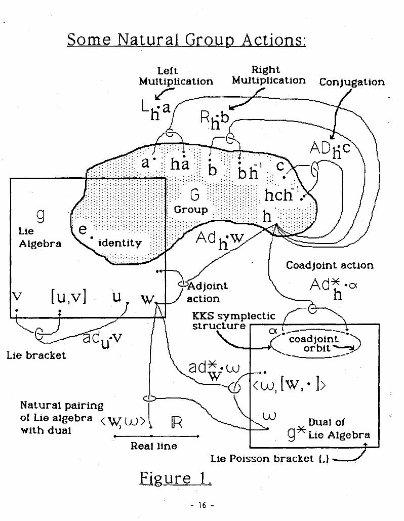